PAC-Bayesian bounds for learning LTI-ss systems with input from empirical loss

Abstract

In this paper we derive a Probably Approxilmately Correct(PAC)-Bayesian error bound for linear time-invariant (LTI) stochastic dynamical systems with inputs. Such bounds are widespread in machine learning, and they are useful for characterizing the predictive power of models learned from finitely many data points. In particular, with the bound derived in this paper relates future average prediction errors with the prediction error generated by the model on the data used for learning. In turn, this allows us to provide finite-sample error bounds for a wide class of learning/system identification algorithms. Furthermore, as LTI systems are a sub-class of recurrent neural networks (RNNs), these error bounds could be a first step towards PAC-Bayesian bounds for RNNs.

I Introduction

Linear time invariant (LTI) state-space models have been widely used in control and econometric applications to model time-series and have rich literature on learning (classically called identification)[1].

In this paper, we present PAC-Bayesian type bounds on learning LTI systems from data generated by LTI system driven by zero-mean, i.i.d., Gaussian or sub-Gaussian noise.

The Probably Approximately Correct (PAC)-Bayesian framework, provides theoretical guarantees (with arbitrary high probability) on the difference between learning from infinite amount of data, and learning from finite empirical data, see [2, 3, 4, 5, 6, 7, 8].

Motivation PAC and PAC-Bayesian bounds have been a major tool for analyzing learning algorithms. They provide bounds on the generalization error in terms of the empirical error, in a manner which is independent of the learning algorithm. Hence, these bounds can be used to analyze and explain a wide variety of learning algorithms. Moreover, by minimizing the error bound, new, theoretically well-founded learning algorithms can be formulated. In particular, PAC-Bayesian error bounds turned out to be useful for providing non-vacuous error bounds for neural networks [9].

While there is a wealth of literature on PAC [10] and PAC-Bayesian [3, 2], bounds for static models, much less is known on dynamical systems.

Traditionally, the literature on LTI systems [1] has focused on statistical consistency. More recently, several results have appeared on finite-sample bounds for learning LTI systems, but they are valid only for specific learning algorithms or for very limited subclasses [11, 12, 13],

Contribution In this paper we consider stochastic LTI state-space representations (LTI systems for short) in innovation form. In accordance with the standard practice in system identification, we view stochastic LTI systems as predictors, which take past inputs and outputs and generate predictions for the current output. We assume that the data used for learning (system identification) are generated by stochastic LTI systems in innvation form too. Learning/identifying an LTI system is then amounts to finding the best predictor, i.e., the predictor which results in the smallest prediction error for the training data, i.e., in the smalled empirical loss However, for decision making (fault detection,control, etc.), the quality of the learned model is determined by the generalization error, i.e., the average prediction error for future, unseen data. The PAC-Bayesian bound of this paper says that with a high probability (probability $1-\delta$), the generalization error is smaller than the empirical loss plus a an error term. The error term depends on the number of data points $N$ and on parameter (learning rate $\lambda$). In this paper we provide explicit formulas for the error term. We show that the error term converges to a constant as $N\rightarrow\infty$. The constant depends on the confidence level $\delta$ and the distance between prior and posterior densities on models. If we assume that the data used for learning is generated by an LTI system with bounded noise, we can show that the error term converges to $0$ as $N\rightarrow\infty$. The rate of convergence is $O(\frac{1}{\sqrt{N}})$, which is consistent with most of finite-sample bounds available in the literature for various, not necessarily LTI, models. This suggests that the obtained error bound is likely to be asymptotically sharp for bounded signals.

Related work The related literature can be divided into the following categories.
Generalization bounds for RNNs. PAC bounds for RNN were developed in [14, 15, 16] using VC dimension, and in [17, 16] using Rademacher complexity, and in [18] using PAC-Bayesian bounds approach. However, all the cited papers assume noiseless models, a fixed number of time-steps, that the training data are i.i.d sampled time-series, and the signals are bounded. In contrast, we consider (1) noisy models, (2) prediction error defined on infinite time horizon, (3) only one single time series available for training data, and (4) unbounded signals. Moreover, several papers [14, 15, 19] assume Lipschitz loss functions, while we use quadratic loss function.

Finite-sample bounds for system identification of LTI systems. Guarantees for asymptotic convergence of learning algorithms is a classical topic in system identification [1]. Recently, several publications on finite-sample bounds for learning linear dynamical systems were derived, without claiming completeness [20, 21, 11, 13, 22, 23, 24, 25, 26]. First, all the cited papers propose a bound which is valid only for models generated by a specific learning algorithm. In particular, these bounds do not relate the generalization loss with the empirical loss for arbitrary models, i.e., they are not PAC(-Bayesian) bounds. This means that in contrast to the results of this paper, the bounds of the cited papers cannot be use for analyzing algorithms others than for which they were derived. Second, many of the cited papers do not derive bounds on the infinite horizon prediction error. More precisely, [13, 26, 22, 25, 27] provided error bounds for the difference of the first $T$ Markov-parameters of the estimated and true system for a specific identification algorithm. However, in order to characterize the infinite horizon prediction error, we need to take $T=\infty$. For $T=\infty$ the cited bounds become infinite, i.e., vacuous. In addition, in contrast to the present paper, [13, 26, 20] deals only with the deterministic part of the stochastic LTI, [25] deals only with the stochastic part.

PAC-Bayesian bounds for state-space representation. In [28] learning of stochastic differential equations without inputs was considered and it was assumed that several independently sampled time-series were available for learning. In contrast, in this paper we deal with discrete-time systems with inputs and the learning takes place from a single time-series. In [29] learning of general Markov-chains was considered, but the state of the Markov-chain was assumed to be observable and no inputs were considered. The learning problem of [29] is thus different from the one considered in this paper.

In [30] PAC-Bayesian error bounds were developed for autonomous LTI state-space systems without exogenous input. In contrast to [30], in the current paper we consider systems with exogenous inputs. Moreover, the error bound of this paper is much tighter than that of [30]: in contrast to [30], with the growth of the number of observations, the error bounds of this paper converge either to zero (in the case of bounded innovation noise) or to a constant involving KL-divergence. Finally, the proof technique is completely different from that of [30].

Paper Outline We start by defining the problem formulation in Section II, where all the assumptions and important quantities are defined. Then we will discuss the PAC-Bayesian framework in Section III, then we will present the main results of the paper in Section IV, then we will present some auxiliary results for systems driven by bounded noise in Section V, We will finish off with a short numerical example in Section VI. Finally, we will have the conclusion in Section VII.

II Problem formulation

Notation and terminology

We occasionally use $\triangleq$ to denote ”defined by”. Let $\mathbf{F}$ denote a $\sigma$-algebra on the set $\Omega$ and $\mathbf{P}$ be a probability measure on $\mathbf{F}$. Unless otherwise stated all probabilistic considerations will be with respect to the probability space $(\Omega,\mathbf{F},\mathbf{P})$, and we let $\mathbf{E}(\mathbf{z})$ denote expectation of the stochastic variable $\mathbf{z}$. We use bold face letters to indicate stochastic variables/processes. Each euclidean space is associated with the topology generated by the 2-norm $\|\cdot\|_{2}$, and the Borel $\sigma$-algebra generated by the open sets. The induced matrix 2-norm is also denoted $\|\cdot\|_{2}$. We say that a random variable $\mathbf{z}$ taking values in $\mathbb{R}^{n}$ is essentially bounded, if for some constant $C>0$, $\|\mathbf{z}\|_{2}<C$ holds with probability one.

A stochastic linear-time invariant (LTI) systems with inputs in state-space form [31, Chapter 17] is a dynamical system of the form

$$\begin{split}\mathbf{x}(t+1)=A\mathbf{x}(t)+B\mathbf{u}(t)+\bm{\nu}(t),\\ \mathbf{y}(t)=C\mathbf{x}(t)+D\mathbf{u}(t)+\bm{\eta}(t)\end{split}$$ (1)

defined for all $t\in\mathbb{Z}$, where $A,B,C,D$ are $n\times n$, $n\times n_{u}$, $n_{y}\times n$ and $n_{y}\times n_{u}$ matrices respectively, $A$ is a Schur matrix (a square matrix with all its eigenvalues inside the unit disk), $\bm{\nu},\bm{\eta}$ are zero-mean Gaussian i.i.d processes, $\mathbf{u}$, $\mathbf{x}$, are zero-mean stationary Gaussian processes, $\mathbf{u}(t)$ and $\begin{bmatrix}\bm{\eta}^{T}(t),\bm{\nu}^{T}(t)\end{bmatrix}^{T}$ are independent, and $\mathbf{x}(t)$ and $\begin{bmatrix}\bm{\nu}^{T}(t),\bm{\eta}^{T}(t)\end{bmatrix}^{T}$ are independent. The process $\mathbf{x}$ is called the state process, $\bm{\nu}$ is called the process noise and $\bm{\eta}$ is the measurement noise. If $B,D$ are absent from (1), then we say that (1) is an autonomous stochastic LTI system

Let us fix stochastic processes $\mathbf{y}(t)\in\mathbb{R}^{n_{\mathbf{y}}}$, and ${\mathbf{u}}(t)\in\mathbb{R}^{n_{\mathbf{u}}}$, that share a time axis $t\in{\mathbb{Z}}$, that is, for any $t\in\mathbb{Z}$, $\mathbf{y}(t):\Omega\to{\mathbb{R}}^{n_{\mathbf{y}}};\omega\mapsto\mathbf{y}(t)(\omega)$, and $\mathbf{u}(t):\Omega\to{\mathbb{R}}^{n_{\mathbf{u}}};\omega\mapsto{\mathbf{u}}(t)(\omega)$ are random vectors on $(\Omega,\mathbf{F},\mathbf{P})$. The goal is to estimate $\mathbf{y}(t)$ from current and past values of ${\mathbf{u}}(t)$, for this we need a structure connecting ${\mathbf{y}}(t)$ and ${\mathbf{u}}(t)$, thus we have

Assumption II.1

Let $\mathbf{y}(t)$ and $\mathbf{u}(t)$ be generated by an autonomous stochastic LTI system

$$\mathbf{x}(t+1) =A_{g}\mathbf{x}(t)+K_{g}\mathbf{e}_{g}(t),$$ (2a)

$$\begin{bmatrix}\mathbf{y}(t)\\ \mathbf{u}(t)\end{bmatrix} =C_{g}\mathbf{x}(t)+\mathbf{e}_{g}(t)$$ (2b)

where $A_{g}\in\mathbb{R}^{n\times n},K_{g}\in\mathbb{R}^{n\times m},C_{g}\in\mathbb{R}^{m\times n}$ for $n>0$, $m=n_{y}+n_{u}\geq 2$ and $\mathbf{x}$, $\mathbf{y}$ and $\mathbf{e}_{g}$ are stationary, zero-mean, and jointly Gaussian stochastic processes. Furthermore, we require that $A_{g}$ and $A_{g}-K_{g}C_{g}$ are Schur (all its eigenvalues are inside the open unit circle), that $\mathbf{e}_{g}(t)$ is white noise uncorrelated with $\mathbf{x}(t-k)$, with covariance $\mathbf{E}[\mathbf{e}_{g}(t)\mathbf{e}_{g}^{T}(t)]=Q_{e}$, and that $\mathbf{e}_{g}$ is the innovation process (see [31] for definition) of $\begin{bmatrix}\mathbf{y}^{T}&\mathbf{u}^{T}\end{bmatrix}^{T}$. We identify the system (2) with the tuple $\Sigma_{gen}\triangleq(A_{g},K_{g},C_{g},I)$;

Note: For learning, we assume to have the training data set $\mathcal{D}_{N}=\{\{\mathbf{y}(s),{\mathbf{u}}(s)\}\}_{s=0}^{N-1}$, i.e. a single trajectory of $[\mathbf{y}^{T}(t),{\mathbf{u}}^{T}(t)]^{T}$, but no knowledge of the matrices $A_{g},K_{g},C_{g}$ and noise process $\mathbf{e}_{g}$. The system (2) only defines the assumptions on the data generating process.

The goal is to use the past and present of ${\mathbf{u}}(t)$, or past of $\mathbf{y}(t)$, to estimate $\mathbf{y}(t)$. Note that $\mathbf{y}$ and ${\mathbf{u}}$ are stationary processes by [32, Theorem 1.4]. Moreover, from classical theory of LTI systems it follows that $\mathbf{y}(t)$ and ${\mathbf{u}}(t)$, $t\in\mathbb{Z}$ are essentially bounded if the noise $\mathbf{e}_{g}(s)$ is essentially bounded for all $s\in\mathbb{Z}$

That is we wish to consider LTI predictors,

$$\hat{\mathbf{x}}(t+1) =\hat{A}\hat{\mathbf{x}}(t)+\hat{B}{\mathbf{u}}(t)+\hat{L}\mathbf{y}(t),~{}\hat{\mathbf{x}}(0)=0$$ (3a)

$$\hat{\mathbf{y}}(t) =\hat{C}\hat{\mathbf{x}}(t)+\hat{D}{\mathbf{u}}(t)$$ (3b)

where matrices $\hat{A},\hat{B},\hat{L},\hat{C},\hat{D}$ are of appropriate size, and $\hat{A}$ is Schur (all its eigenvalues are inside the unit disk).

Note: In this paper, we will allow a more general form of predictors, where $\hat{L}$ can be set to 0, i.e. we may wish to estimate $\mathbf{y}(t)$ only from measurements ${\mathbf{u}}(t)$, when past values of the process $\mathbf{y}(t)$ is not available. In order to accommodate this let us define a stochastic process $\mathbf{w}(t)\in{\mathbb{R}}^{n_{\mathbf{w}}}$, by two cases

• $\mathbf{w}(t)=\begin{bmatrix}\mathbf{y}^{T}(t)&{\mathbf{u}}^{T}(t)\end{bmatrix}^{T}$, $n_{\mathbf{w}}=n_{\mathbf{y}}+n_{\mathbf{u}}$

• $\mathbf{w}(t)={\mathbf{u}}(t)$, $n_{\mathbf{w}}=n_{\mathbf{u}}$

Note that, one can define $\mathbf{w}(t)$, to consist of some of the components of $\mathbf{y}(t)$, i.e. $\mathbf{w}(t)$ does not need to contain all of $\mathbf{y}$.

Class of predictors (hypotheses) In this paper, we will be interested in the following hypothesis class, consisting of predictors realizable by LTI systems.

Assumption II.2 (Parameterised hypothesis class)

The hypothesis class $\mathcal{F}$ is a parametrized set of LTI predictors, with $\Sigma(\theta)=(\hat{A}(\theta),\hat{B}(\theta),\hat{C}(\theta),\hat{D}(\theta))$:

$$\hat{{\mathbf{x}}}(t+1) =\hat{A}\hat{{\mathbf{x}}}(t)+\hat{B}{\mathbf{w}}(t),\;\hat{{\mathbf{x}}}(0)=0,$$ (4a)

$$f_{\Sigma(\theta)}(\{{\mathbf{w}}(s)\}_{s=0}^{t}) =\hat{C}\hat{{\mathbf{x}}}(t)+\hat{D}{\mathbf{w}}(t).$$ (4b)

$$\mathcal{F}=\{f_{\Sigma(\theta)}\mid\gamma(\hat{A}(\theta))<1,\;\theta\in\Theta\}$$

with $\gamma(\hat{A}(\theta))$ the spectral radius of $\hat{A}(\theta)$, i.e. the largest modulus of eigenvalues of $\hat{A}(\theta)$. Set $\Theta\subset{\mathbb{R}}^{n_{\theta}}$ is a compact set, and $\hat{A}(\theta)$,$\hat{B}(\theta),\hat{C}(\theta),\hat{D}(\theta)$ are continuous functions of $\theta$ taking values in the sets of $\hat{n}\times\hat{n}$, $\hat{n}\times n_{w}$, $n_{y}\times\hat{n}$ and $n_{y}\times n_{w}$ matrices respectively. If $\mathbf{w}(t)=[\mathbf{y}^{T}(t),{\mathbf{u}}^{T}(t)]^{T}$, then $\hat{D}=[0,\hat{D}_{\mathbf{u}}]$ for some $n_{y}\times n_{u}$ matrix $\hat{D}_{\mathbf{u}}$, i.e., $\hat{D}\mathbf{w}(t)$ depends only on $\mathbf{u}(t)$.

We will identify the system (4) with the tuple $(\hat{A},\hat{B},\hat{C},\hat{D})$. For the sake of notation, throughout the paper we will use $f$, to denote $f_{\Sigma(\theta)}$, for some arbitrary $\theta\in\Theta$.

Under assumption II.2, we can use probability densities on the set of predictors $\mathcal{F}$. The latter will be essential for using the PAC-Bayesian framework.

Next, we define the notions of empirical and generalization loss for predictors which are realized by LTI systems.

Assumption II.3 (Quadratic loss function)

We will consider quadratic loss functions $\ell:\mathbb{R}^{n_{y}}\times\mathbb{R}^{n_{y}}\ni(y,y^{\prime})\mapsto\|y-y^{\prime}\|_{2}^{2}=(y-y^{\prime})^{T}(y-y^{\prime})\in[0,\infty)$.

The empirical loss of a predictor for the data $\mathcal{D}_{N}=\{\mathbf{y}(t),\mathbf{w}(t)\}_{t=0}^{N}$ is defined as follows: we define the random variable

$$\hat{\mathbf{y}}_{f}(t\mid s)\triangleq f(\mathbf{w}(s),\ldots,\mathbf{w}(t))$$

which represents the estimate of $\mathbf{y}(t)$ based on random variables $\{\mathbf{w}(s),\ldots,\mathbf{w}(t)\}$ . The empirical loss for a predictor $f$ and processes $(\mathbf{y},\mathbf{w})$ is defined by

$$\hat{\mathcal{L}}_{N}(f)\triangleq\frac{1}{N}\sum_{i=0}^{N-1}\ell(\hat{\mathbf{y}}_{f}(i\mid 0),\mathbf{y}(i)).$$ (5)

The definition of the generalization loss is a bit more involved. Namely, we are using varying number of inputs for predictions and hence the expectation $\mathbf{E}[\ell(\hat{\mathbf{y}}_{f}(t\mid 0),\mathbf{y}(t))]$ depends on $t$. This will hold true even if the processes $\mathbf{y}$ and $\mathbf{w}$ are stationary. Note that this issue is specific for state-space models: autoregressive models always use the same number of inputs to make a prediction, see Remark II.1. In this paper we will opt for looking at the case when the size of the past used for the prediction is infinite. To this end, we need the following result from [33].

Lemma II.1 ([33])

The limit $\hat{\mathbf{y}}_{f}(t)=\lim_{s\rightarrow-\infty}\hat{\mathbf{y}}_{f}(t\mid s)$ exists in the mean-square sense for all $t$, the process $\hat{\mathbf{y}}_{f}(t)$ is stationary, and $\mathbf{E}[\ell(\hat{\mathbf{y}}_{f}(t),\mathbf{y}(t))]=\lim_{s\rightarrow-\infty}\mathbf{E}[\ell(\hat{\mathbf{y}}_{f}(t\mid s),\mathbf{y}(t))]$.

This motivates us to introduce the quantity

$$\mathcal{L}(f)=\mathbf{E}[\ell(\hat{\mathbf{y}}_{f}(t),\mathbf{y}(t))]=\lim_{s\rightarrow-\infty}\mathbf{E}[\ell(\hat{\mathbf{y}}_{f}(t\mid s),\mathbf{y}(t))]$$

which is called the generalization loss of the predictor $f$ when applied to process $(\mathbf{y},\mathbf{w})$.

Intuitively, $\hat{\mathbf{y}}_{f}(t)$ can be interpreted as the prediction of $\mathbf{y}(t)$ generated by the predictor $f$ based on all (infinite) past and present values of $\mathbf{w}$. As stated in Lemma II.1 we consider the special case when $\hat{\mathbf{y}}_{f}(t)$ is the mean-square limit of $\hat{\mathbf{y}}_{f}(t\mid s)$ as $s\rightarrow-\infty$. Clearly, for large enough $t-s$, the empirical loss, is close to the generalization loss. In fact, it is standard practice in learning dynamical systems [1] to use $\mathcal{L}(f)$ as the measure of fitness of the predictor. With these definitions in mind, the learning problem considered in this paper can be stated as follows.

Problem II.1 (Learning problem)

Compute a predictor $f\in\mathcal{F}$ from a sample $\mathcal{D}_{N}=\{\mathbf{y}(t)(\omega),{\mathbf{w}}(t)(\omega)\}_{t=0}^{N}$ of the random variables $\{\mathbf{y}(t),\mathbf{w}(t)\}_{t=0}^{N}$ such that the generalization loss $\mathcal{L}(f)$ is small.

Remark II.1

It is known [1, Section 4.2] that the LTI system (3) can be rewritten as an ARX model:

$$\hat{\mathbf{y}}_{f}(t|s)=\sum_{i=1}^{n}\hat{\gamma}_{i}\hat{\mathbf{y}}_{f}(t-i|s)+\sum_{i=0}^{n-1}\hat{\eta}_{i}\mathbf{w}(t-i)$$ (6)

At a first glance this is similar to classical ARX predictors, where $\hat{\mathbf{y}}(t)=\sum_{k=1}^{n}\hat{\alpha}_{k}\mathbf{y}(t-k)+\sum_{i=0}^{n-1}\hat{\beta}_{i}\mathbf{w}(t-i)$ where $\mathbf{y}$ is predicted based on the last $n$ values of $\mathbf{y}$ and $\mathbf{w}$. However, in contrast to classical ARX models, in (6) we do not use the past values of $\mathbf{y}$, but the past values of the prediction $\hat{\mathbf{y}}_{f}$. This difference has significant consequences, in particular, it means that the previous results [34] do not apply. Note that [35, 36] studied autoregressive models without inputs (nonlinear AR models), so those results are not applicable either. In fact, the problem of learning LTI systems with inputs, or, which is almost equivalent, learning LTI predictors, is essentially equivalent to learning ARMA models, and the latter is much more involved than learning ARX models.

III PAC-Bayesian Framework

Below we present the adaptation of the PAC-Bayesian framework for LTI systems. To this end, let $B_{\Theta}$ be the $\sigma$-algebra of Lebesque-measurable subsets of the parameter set $\Theta\subseteq\mathbb{R}^{n_{\theta}}$, and $m$ denote the Lebesque measure on $\mathbb{R}^{n_{\theta}}$. We then define

$$\underset{f\sim\rho}{E}g(f)\triangleq\int_{\theta\in\Theta}\rho(\theta)g(f_{\Sigma(\theta)})dm(\theta)$$ (7)

with $\rho$ a probability density function on the measure space $(\Theta,B_{\theta},m)$, and $g:\mathcal{F}\rightarrow\mathbb{R}$ a map such that $\Theta\ni\theta\mapsto g(f_{\theta})$ is measurable and absolutely integrable. The essence of the PAC-Bayesian approach is to prove that for any density $\pi$ on $\mathcal{F}$, and any $\delta\in(0,1]$,

$$\mathbf{P}\Big{(}\Big{\{}\omega\in\Omega\mid\forall\hat{\rho}\in\mathcal{M}_{\pi}:\underset{f\sim\hat{\rho}}{E}\mathcal{L}(f)\leq\kappa(\omega) \Big{\}}\Big{)}>1-\delta,$$ (8)

with

$$\kappa(\omega)=\underset{f\sim\hat{\rho}}{E}\hat{\mathcal{L}}_{N}(f)(\omega)+r_{N}$$

$\mathcal{M}_{\pi}$ the set of all absolutely continuous densities w.r.t $\pi$, and $r_{N}=r_{N}(\pi,\hat{\rho},\delta)$ an error term. That is, the PAC-Bayesian bound holds for every posterior $\hat{\rho}$ in $\mathcal{M}_{\pi}$, simultaneously.

We may think of $\pi$ as a prior distribution density function and $\hat{\rho}$ as any candidate to a posterior distribution on the space of predictors. The inequality (8) says that the average generalization loss for models sampled from the posterior distribution is smaller than the average empirical loss for the posterior distribution plus the error terms $r_{N}$.

A learning algorithm can be thought of as fixing a prior $\pi$ and then choosing a posterior $\hat{\rho}$ for which $\kappa(\omega)$ is small. Moreover, $\kappa(\omega)$ can be viewed as a cost function involving the empirical loss and the regularization term $r_{N}$. The learned model is either sampled from the posterior density $\hat{\rho}$, or it is chosen as the one with maximal likelihood w.r.t. $\hat{\rho}$. Inequality (8) then gives guarantees on the generalization loss of the learned model. For more details on using PAC-Bayesian bounds see [3] For (8) to be useful, the term $r_{N}$ should converge to a small constant, preferably zero, as $N\rightarrow\infty$, and to be decreasing in $\delta$. The most common way of expressing the error term $r_{N}$, is based on Donsker-Varadhan’s change of measure [7, Theorem 3]:

$$r_{N}=\dfrac{1}{\lambda}\!\left[D_{\mathrm{KL}}(\hat{\rho}\|\pi)+\ln\dfrac{1}{\delta}+\Psi_{\pi}(\lambda,N)\right],$$ (9)

where $\lambda>0$ and $D_{\mathrm{KL}}(\hat{\rho}\mid\pi)\triangleq E_{f\sim\hat{\rho}}\ln\frac{\hat{\rho}(f)}{\pi(f)}$ is the KL-divergence between $\pi$ and $\hat{\rho}$, and

$$\Psi_{\pi}(\lambda,N)\triangleq\ln E_{f\sim\pi}\mathbf{E}[e^{\lambda(\mathcal{L}(f)-\hat{\mathcal{L}}_{N}(f))}]$$ (10)

That is, $r_{N}$ involves the KL-divergence and a free parameter $\lambda$. The density which minimizes $\kappa(\omega)$, with $r_{N}$ from (9) is known as the Gibbs-posterior [3] and it can be explicitly computed, i.e.

$$\rho_{\text{Gibbs}}(f) \triangleq Z^{-1}\pi(f)\exp(-\lambda\hat{\mathcal{L}}_{N}(f)),$$ (11)

$$Z \triangleq E_{f\sim\pi}\exp(-\lambda\hat{\mathcal{L}}_{N}(f)).$$

The disadvantage of this approach is that it is difficult to bound $\Psi_{\pi}(\lambda,N)$, since it involves bounding higher-order moments

$$\mathbf{E}[|\mathcal{L}(f)-\hat{\mathcal{L}}_{N}(f)|^{r}],\quad r\in{\mathbb{N}}$$ (12)

One can also use PAC-Bayesian bounds, in order to choose the prior $\pi$ or the hypothesis class $\mathcal{F}$, s.t. the difference between generalised loss and empirical loss is within some acceptable level, i.e.

$$E_{f\sim\rho}\left(\mathcal{L}(f)-\hat{\mathcal{L}}_{N}(f)\right)\leq r_{N}(\lambda,\pi)\leq\epsilon$$ (13)

then it is only a matter of choosing $\pi,\lambda,\mathcal{F}$, s.t. $r_{N}(\lambda,\pi)\leq\epsilon$, after which one can proceed with more standard Bayesian learning approach on just the empirical loss $\hat{\mathcal{L}}_{N}(f)$.

In the next section, we will apply a simple trick, which will allow us to upper-bound higher-order moments.

IV Main Results

In this paper we derive PAC-Bayesian bounds (8) for LTI systems. The main idea is to use the change of measure inequality from [7, Theorem 3]. The major challenge is to bound the corresponding moment generating function/higher-order moments of $(\mathcal{L}(f)-\hat{\mathcal{L}}_{N}(f))$. However this brings some technical challenges. Namely, the processes involved are not i.i.d.. Moreover, they are not bounded, and the quadratic loss function is not Lipschitz. In addition, the empirical loss $\hat{\mathcal{L}}_{N}(f)$ is not an unbiased estimate of the generalization loss $\mathcal{L}(f)$. This is specific to state-space representations, for auto-regressive models considered in [35, 36, 37] this problem does not occur. All these issues make it impossible to directly apply existing techniques [35, 36, 37].
As the first step, temporarily we replace the empirical loss $\hat{\mathcal{L}}_{N}(f)$ by

$$V_{N}(f)\triangleq\frac{1}{N}\sum_{i=0}^{N-1}(\mathbf{y}(i)-\hat{\mathbf{y}}_{f}(i))^{2}$$ (14)

where the finite-horizon prediction $\hat{\mathbf{y}}_{f}(t\mid 0)$ is replaced by the infinite horizon prediction $\hat{\mathbf{y}}_{f}(t)$ defined in Lemma II.1. The advantage of $V_{N}(f)$ over $\hat{\mathcal{L}}_{N}(f)$ is that $V_{N}(f)$ is an unbiased estimate of the generalization loss $\mathcal{L}(f)$, i.e., $\mathbf{E}[V_{N}(f)]=\mathcal{L}(f)$. Indeed, since $\mathbf{y}(t)-\hat{\mathbf{y}}_{f}(t)$ is a stationary process, $E[\|\mathbf{y}(i)-\hat{\mathbf{y}}_{f}(i)\|^{2}_{2}]=\mathcal{L}(f)$ does not depend on $i$, and hence $\mathbf{E}[V_{N}(f)]=\frac{1}{N}\sum_{i=0}^{N-1}E[\|\mathbf{y}(i)-\hat{\mathbf{y}}_{f}(i)\|^{2}_{2}]=\mathcal{L}(f)$. hence, usual techniques for deriving error bounds are easier to extend to $V_{N}(f)$ than to $\hat{\mathcal{L}}_{N}(f)$. Moreover, , from Lemma B.7 in Appendix B of the supplementary material, it follows that $\hat{\mathcal{L}}_{N}(f)-V_{N}(f)$ converges to zero as $N\rightarrow\infty$ in the mean sense. In order to derive upper bounds on the errors of the type (9), we will first derive upper bounds of the type (9), for $\mathcal{L}(f)-V_{N}(f)$, secondly we will derive upper bounds for $V_{N}(f)-\hat{\mathcal{L}}_{N}(f)$, then we will combine them using union bound. Doing this might seem counter-productive, however it is significantly easier to bound moments, $\mathbf{E}[(\mathcal{L}(f)-V_{N}(f))^{r}]$, and $\mathbf{E}[(V_{N}(f)-\hat{\mathcal{L}}_{N}(f))^{r}]$

For every predictor $f$ we define the following constants.

Definition IV.1 (Constants $\bar{G}_{f}(f),G_{e}(f)$)

Let $f=(\hat{A},\hat{B},\hat{C},\hat{D})$ be a predictor. Let $A_{g},K_{g},C_{g}$ be the matrices of the data generator from Assumption II.1. Define the matrices $(A_{e},K_{e},C_{e},D_{e})$ as $D_{e}=I-\hat{D}_{w}$,

$$A_{e}=\begin{bmatrix}A_{g}&0\\ \hat{B}C_{w}&\hat{A}\end{bmatrix},~{}K_{e}=\begin{bmatrix}K_{g}\\ \hat{B}_{w}\end{bmatrix},~{}C_{e}=\begin{bmatrix}(C_{1}-\hat{D}C_{w})^{T}\\ -\hat{C}^{T}\end{bmatrix}^{T},$$

where $C_{g}=\begin{bmatrix}C_{1}^{T}&C_{2}^{T}\end{bmatrix}^{T}$ and $C_{1}$ has $n_{y}$ rows and $C_{2}$ has $n_{u}$ rows; and $(C_{w},\hat{B}_{w},\hat{D}_{w})=(C_{2},\begin{bmatrix}0&\hat{B}\end{bmatrix},\begin{bmatrix}0&\hat{D}\end{bmatrix})$ if $\mathbf{w}=\mathbf{u}$, and $(C_{w},\hat{B}_{w},\hat{D}_{w})=(C_{g},\hat{B},\hat{D})$, if $\mathbf{w}=\begin{bmatrix}\mathbf{y}^{T}&\mathbf{u}^{T}\end{bmatrix}^{T}$. Choose for all $f\in\mathcal{F}$, $\hat{M}(f)>1$, and $\hat{\gamma}(f)\in[\hat{\gamma}^{*}(f),1)$, such that $\|\hat{A}^{k}\|_{2}\leq\hat{M}(f)\hat{\gamma}^{k}(f)$, with $\hat{\gamma}^{*}(\hat{A})$ the spectral radius of $\hat{A}$. With these definitions,

$$G_{e}(f)=\|(A_{e},K_{e},C_{e},D_{e})\|_{\ell_{1}}\triangleq\|D_{e}\|_{2}+\sum_{k=0}^{\infty}\|C_{e}A_{e}^{k}K_{e}\|_{2}$$

$$\|\Sigma_{gen}\|_{\ell_{1}}=1+\sum_{k=0}^{\infty}\|C_{g}A_{g}^{k-1}K_{g}\|_{2}$$

$$\bar{G}_{gen}=\|\Sigma_{gen}\|_{\ell_{1}}^{2}\mu_{\max}(Q_{e})$$

$$\bar{G}_{f}(f)=\left(1+\|\hat{D}\|+\frac{\hat{M}\|\hat{B}\|\|\hat{C}\|}{1-\hat{\gamma}}\right)\frac{\hat{M}\|\hat{C}\|\|\hat{B}\|}{(1-\hat{\gamma})^{1.5}}$$

The interpretation of the various terms appearing in Definition IV.1 is as follows.

Remark IV.1 (Interpretation of constants)

The matrices $A_{e},K_{e},C_{e},D_{e}$ represent the LTI system driven by the innovation process $\mathbf{e}_{g}$ of $(\mathbf{y}^{T},\mathbf{w}^{T})^{T}$, output of which is $\mathbf{y}-\hat{\mathbf{y}}_{f}$, i.e.,

$$\begin{split}\tilde{\mathbf{x}}(t+1)=A_{e}\tilde{\mathbf{x}}(t)+K_{e}\mathbf{e}_{g}(t),\\ \mathbf{y}(t)-\hat{\mathbf{y}}_{f}(t)=C_{e}\tilde{\mathbf{x}}(t)+D_{e}\mathbf{e}_{g}(t)\end{split}$$ (15)

The term $\bar{G}_{\text{gen}}$ depends only on the data generator system (2), and characterises the scaling of $\mathbf{y},{\mathbf{u}}$

The term $\bar{G}_{f}(f)$ depends only the predictor $f$, and should be interpreted similarly to $\|(\hat{A},\hat{B},\hat{C},\hat{D})\|_{\ell_{1}}^{2}$.

Theorem IV.1

Let $\mathcal{M}_{\pi}$ denote the set of all absolutely continuous densities w.r.t $\pi$. Then for any density $\pi$ on hypothesis class $\mathcal{F}$, any $\delta\in(0,1]$, and

$$0<\lambda<\Big{(}\sup_{f\in\mathcal{F}}\max\{8(n_{u}+n_{y})\bar{G}_{gen}\bar{G}_{f}(f),\\ 6(n_{u}+n_{y}+1)n_{y}\mu_{\max}(Q_{e})G_{e}(f)^{2}\}\Big{)}^{-1}$$ (16)

the following inequality holds with probability at least $1-2\delta$

$$\forall\rho\in\mathcal{M}_{\pi}:\quad E_{f\sim\hat{\rho}}\mathcal{L}(f)\leq\mathbb{E}_{f\sim\hat{\rho}}\hat{\mathcal{L}}_{N}(f)+r_{N}(\lambda,N),$$ (17)

with

$$r_{N}(\lambda,N) \triangleq\dfrac{1}{\lambda}\!\left[D_{\mathrm{KL}}(\hat{\rho}\|\pi)+\ln\dfrac{1}{\delta}+\widehat{\Psi}_{\pi}(\lambda,N)\right]$$ (18)

$$\widehat{\Psi}_{\pi}(\lambda,N) \triangleq\frac{1}{2}\left(\widehat{\Psi}_{\pi,1}(\lambda,N)+\widehat{\Psi}_{\pi,2}(\lambda,N)\right)$$ (19)

$$\widehat{\Psi}_{\pi}(\lambda,N) \geq\Psi_{\pi}(\lambda,N)=\ln E_{f\sim\pi}\mathbf{E}[e^{\lambda(\mathcal{L}(f)-\hat{\mathcal{L}}_{N}(f))}]$$

and

$$\widehat{\Psi}_{\pi,1}(\tilde{\lambda},N) \triangleq\ln E_{f\sim\pi}\left(1+\frac{1}{N}C_{1}(f,\lambda)\right)$$ (20)

$$\widehat{\Psi}_{\pi,2}(\tilde{\lambda},N) \triangleq\ln E_{f\sim\pi}\left(1+\frac{1}{\sqrt{N}}C_{2}(f,\lambda)\right)$$ (21)

$$C_{1}(f,\lambda) \triangleq\frac{2(m+1)!\left(6\lambda n_{y}\mu_{\max}(Q_{e})G_{e}(f)^{2}\right)^{2}}{(1-6(m+1)\lambda n_{y}\mu_{\max}(Q_{e})G_{e}(f)^{2})}$$ (22)

$$C_{2}(f,\lambda) \triangleq\frac{8(m!)\lambda\bar{G}_{gen}\bar{G}_{f}(f)}{1-8\lambda m\bar{G}_{gen}\bar{G}_{f}(f)}$$ (23)

For proof of Theorem IV.1, see Proof A.17, in the Appendix.

Note that, as $N\to\infty$ the PAC-Bayesian error $r_{N}\to\frac{1}{\lambda}\left(D_{\mathrm{KL}}(\rho|\pi)+\ln\left(\frac{1}{\delta}\right)\right)$. That is, irrespective of $\rho,\pi$, the error $r_{N}\geq\frac{1}{\lambda}\ln\left(\frac{1}{\delta}\right)$. Usually, one chooses $\lambda=\lambda(N)$ as an increasing function of $N$, which then allows the PAC-Bayesian error to converge to 0. However, since by Theorem IV.1, $\lambda$ is bounded by a constant, we can not control the term $\frac{1}{\lambda}\ln\left(\frac{1}{\delta}\right)$, and $r_{N}>0$ always.

Remark IV.2

Theorem IV.1, holds under assumption II.1, for any distribution of $\mathbf{e}_{g}(t)$, as long as

• $\mathbf{e}_{g}(t)\in\mathbb{R}^{m}$ is zero-mean, i.i.d.,

• $\mathbf{E}\left[\|\mathbf{e}_{g}(t)\|^{2r}\right]\leq 2^{r}\mu_{\max}(Q_{e})^{r}(m+r-1)!$,

• $\sigma(r)\leq 3^{r}\mu_{\max}(Q_{e})^{r}(m+r-1)!$,

with

$$\sigma(r)=\sup_{t,k,j}\mathbf{E}\left[\|\mathbf{e}(t,k,j)\|^{r}_{2}\right],\\ \mathbf{e}(t,k,j)\triangleq\mathbf{E}[\mathbf{e}_{g}(t-k)\mathbf{e}_{g}^{T}(t-j)]-\mathbf{e}_{g}(t-k)\mathbf{e}_{g}^{T}(t-j)$$

That is, Theorem IV.1 holds, for $\mathbf{e}_{g}(t)$, zero mean, i.i.d. with any sub-gaussian distribution.

V Bounded case

If we drop the assumption that $\mathbf{e}_{g}(t)$ has a Gaussian distribution, and only assume that $\mathbf{e}_{g}(t)$ is bounded, we get quite straight-forward PAC-Bayesian bounds.

Assumption V.1

$\mathbf{e}_{g}(t)$ is a zero mean i.i.d. stochastic process, with arbitrary distribution, but for all components $\mathbf{e}_{g,i}(t)$ of $\mathbf{e}_{g}(t)$ $|\mathbf{e}_{g,i}(t)|\leq c_{e}$, for some $c_{e}>0$.

Theorem V.1

Let $\mathcal{M}_{\pi}$ denote the set of all absolutely continuous densities w.r.t $\pi$. Under assumption V.1 it holds true that for any density $\pi$ on hypothesis class $\mathcal{F}$, any $\delta\in(0,1]$, and $\lambda>0$ the following inequality holds with probability at least $1-2\delta$

$$\forall\rho\in\mathcal{M}_{\pi}:\quad E_{f\sim\rho}\mathcal{L}(f)\leq E_{f\sim\rho}\hat{\mathcal{L}}_{N}(f)+\bar{r}_{N}(\lambda,N)$$ (24)

with

$$\bar{r}_{N}(\lambda,N) \triangleq\frac{1}{\lambda}\left[D_{\mathrm{KL}}(\rho||\pi)+\ln\frac{1}{\delta}+\widehat{\Psi}_{c_{e},\pi}(\lambda,N)\right]$$ (25)

$$\widehat{\Psi}_{c_{e},\pi}(\lambda,N) \triangleq\frac{1}{2}\left(\widehat{\Psi}_{c_{e},\pi,1}(\lambda,N)+\widehat{\Psi}_{c_{e},\pi,2}(\lambda,N)\right)$$ (26)

$$\widehat{\Psi}_{c_{e},\pi,1}(\lambda,N) \triangleq\ln E_{f\sim\pi}\left(1+\frac{1}{N}e^{\lambda G_{gen,1}G_{e}(f)^{2}}\right)$$ (27)

$$\widehat{\Psi}_{c_{e},\pi,2}(\lambda,N) \triangleq\ln E_{f\sim\pi}\left(1+\frac{1}{\sqrt{N}}e^{\lambda G_{gen,2}\bar{G}_{f}(f)}\right)$$ (28)

and

$$G_{gen,1} \triangleq 8c_{e}^{2}n_{y}(n_{y}+n_{u})$$ (29)

$$G_{gen,2} \triangleq 4\|\Sigma_{gen}\|_{\ell_{1}}^{2}c_{e}^{2}(n_{y}+n_{u})$$ (30)

For proof of Theorem V.1, see Corollary A.3, in the Appendix. Note that, in this case $\lambda$ is not bounded, and as such we can choose $\lambda=\lambda(N)$ an increasing function of $N$, in order to control the term $\frac{1}{\lambda(N)}\ln\delta^{-1}$. More specifically one can choose

$$\lambda(N) =\frac{\ln\sqrt{N}}{\sup_{f\in\mathcal{F}}\max\{G_{gen,1}G_{e}(f)^{2},G_{gen,2}\bar{G}_{f}(f)\}},$$ (31)

for which, it can be shown that $\lambda^{-1}(N)\Psi_{\pi,c_{e}}(\lambda(N),N)\to 0$, and $\lambda^{-1}(N)\ln\delta^{-1}\to 0$. If one considers $\rho$ independently of $\lambda$, then $\lambda^{-1}(N)D_{\mathrm{KL}}(\hat{\rho}\|\pi)\to 0$, however if one considers Gibbs posteriors (11), which do depend on $\lambda$, then it is hard to say what will happen with $\lambda^{-1}(N)D_{\mathrm{KL}}(\hat{\rho}\|\pi)$. Simulations seem to indicate that if $\lambda(N)$ is any reasonable increasing function of $N$, then $\lambda(N)$ will converge to some problem dependant constant.

The bound above has all the desired properties, but its rate of convergence to zero as $N\rightarrow+\infty$ is very slow. In fact, using [36], the results of Theorem V.1 can be sharpened as follows.

Theorem V.2

Let $\mathcal{M}_{\pi}$ denote the set of all absolutely continuous densities w.r.t $\pi$. Under assumption V.1 it holds true that for any density $\pi$ on hypothesis class $\mathcal{F}$, any $\delta\in(0,1]$, and $\lambda>0$ the following inequality holds with probability at least $1-2\delta$

$$\forall\rho\in\mathcal{M}_{\pi}:\quad E_{f\sim\rho}\mathcal{L}(f)\leq E_{f\sim\rho}\hat{\mathcal{L}}_{N}(f)+\tilde{r}_{N}(\lambda,N)$$ (32)

with

$$\tilde{r}_{N}(\lambda,N) \triangleq\frac{1}{\lambda}\left[D_{\mathrm{KL}}(\rho||\pi)+\ln\frac{1}{\delta}+\tilde{\Psi}_{c_{e},\pi}(\lambda,N)\right]$$ (33)

$$\tilde{\Psi}_{c_{e},\pi}(\lambda,N) \triangleq\frac{1}{2}\left(\tilde{\Psi}_{1}(\lambda,N)+\tilde{\Psi}_{2}(\lambda,N)\right)$$ (34)

$$\tilde{\Psi}_{1}(\lambda,N) \triangleq\ln E_{f\sim\pi}\left(1-C_{1,2}(f)+C_{1,2}(f)e^{\frac{\lambda}{N}C_{1,1}(f)}\right)$$ (35)

$$\tilde{\Psi}_{2}(\lambda,N) \triangleq\ln E_{f\sim\pi}\left(e^{\frac{\lambda^{2}}{N}C_{2}(f)}\right)$$ (36)

and, with $C\triangleq c_{e}\sqrt{n_{u}+n_{y}}$,

$$C_{1,1}(f) \triangleq 2\|\Sigma_{gen}\|_{\ell_{1}}C\bar{G}_{f,2}(f)$$ (37)

$$C_{1,2}(f) \triangleq\bar{G}_{f,1}(f)\|\Sigma_{gen}\|_{\ell_{1}}C$$ (38)

$$C_{2}(f) \triangleq 8(G_{e}(f)+G_{e,1}(f))^{2}C^{2}(4G_{e}(f)C+1)^{2}$$ (39)

$$G_{e,1} \triangleq\|D_{e}\|_{2}+\sum_{k=0}^{\infty}(k+1)\|C_{e}A_{e}^{k}K_{e}\|_{2}$$ (40)

For proof of Theorem V.2, see Proof A.26, in the Appendix. If $\lambda_{N}=\sqrt{N}$ is chosen, then the error bound $\bar{r}_{N}(\lambda_{N})$ above converges to zero as $N\rightarrow\infty$ at a rate $O(\frac{1}{\sqrt{N}})$.

VI Numerical example

For the sake of illustration let us assume that data is generated by

$$\mathbf{x}(t+1) =\begin{bmatrix}0.16&-0.3\\ 0&-0.05\end{bmatrix}\mathbf{x}(t)+\begin{bmatrix}0.33&-0.75\\ 0&-0.09\end{bmatrix}\mathbf{e}_{g}(t)$$

$$\begin{bmatrix}\mathbf{y}(t)\\ {\mathbf{u}}(t)\end{bmatrix} =\begin{bmatrix}1&1\\ 0&1\end{bmatrix}\mathbf{x}(t)+\mathbf{e}_{g}(t),$$

Following the two theorems in the paper, we will consider two cases

• Unbounded innovation noise: $\mathbf{e}_{g}(t)\sim\mathcal{N}(0,Q_{e})$,

  $$Q_{e}=\begin{bmatrix}0.054&0.018\\ 0.018&0.248\end{bmatrix}$$ (41)

• Bounded innovation noise: $\mathbf{e}_{g}(t)$ is distributed according to zero-mean truncated gaussian, s.t. $c_{e}=1$, and

  $$\mathbf{E}[\mathbf{e}_{g}(t)\mathbf{e}_{g}^{T}(t)]\approx Q_{e}$$ (42)

We will assume that the predictors are fully parameterised, i.e. for the case of $\mathbf{w}(t)={\mathbf{u}}(t)$

$$\hat{A}(\theta)=\begin{bmatrix}\theta_{1}&\theta_{2}\\ \theta_{3}&\theta_{4}\end{bmatrix}\;\hat{B}(\theta)=\begin{bmatrix}\theta_{5}\\ \theta_{6}\end{bmatrix}$$

$$\hat{C}(\theta)=\begin{bmatrix}\theta_{7}&\theta_{8}\end{bmatrix}\;\hat{D}(\theta)=\begin{bmatrix}\theta_{9}\end{bmatrix}$$

for the case of $\mathbf{w}(t)=[\mathbf{y}^{T}(t),{\mathbf{u}}^{T}(t)]^{T}$

$$\hat{A}(\theta)=\begin{bmatrix}\theta_{1}&\theta_{2}\\ \theta_{3}&\theta_{4}\end{bmatrix}\;\hat{B}(\theta)=\begin{bmatrix}\theta_{10}&\theta_{5}\\ \theta_{11}&\theta_{6}\end{bmatrix}$$

$$\hat{C}(\theta)=\begin{bmatrix}\theta_{7}&\theta_{8}\end{bmatrix}\;\hat{D}(\theta)=\begin{bmatrix}0&\theta_{9}\end{bmatrix}$$

Thus, with $\Sigma(\theta)=(\hat{A}(\theta),\hat{B}(\theta),\hat{C}(\theta),\hat{D}(\theta))$, we will define our hypothesis class to be

$$\mathcal{F}=\{f_{\Sigma(\theta)}|\gamma(\hat{A}(\theta))<1,\bar{G}_{f}(f)<10,\theta\in{\mathbb{R}}^{11}\}$$

The prior is given by

$$\pi(f)=Z_{\pi}\exp(-\bar{G}_{f}(f))$$ (43)

with $Z_{\pi}$ the normalisation term. This prior will act as regularisation, penalising predictors with high $\ell_{1}$ norms. We will use the Gibbs posterior

$$\rho(f|N)=Z_{\rho}\pi(f)\exp(-\lambda(N)\hat{\mathcal{L}}_{N}(f))$$ (44)

In order to compute the numerical value of $r_{N}$, we can use Markov-Chain Monte-Carlo methods, which means that we only need to be able to evaluate

$$\hat{\pi}(f)=\exp(-\bar{G}_{f}(f))\propto\pi(f)$$ (45)

$$\hat{\rho}(f)=\hat{\pi}(f)\exp(-\lambda\hat{\mathcal{L}}_{N}(f))\propto\rho(f)$$ (46)

More precisely one can approximate $r_{N}$, by only being able to evaluate $\hat{\pi}(f)$ and $\beta(f)\triangleq\frac{\hat{\rho}(f)}{\hat{\pi}(f)}\propto\frac{\rho(f)}{\pi(f)}$

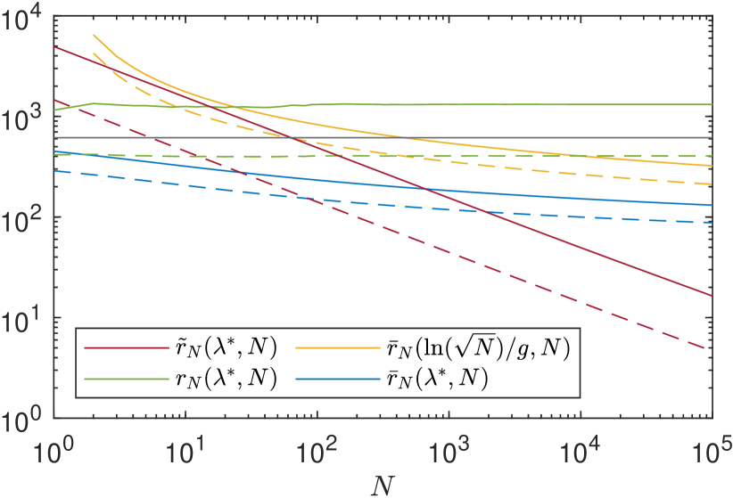
Figure 1: Numerical simulation of both cases (bounded and unbounded noise), solid lines depict case of $\mathbf{w}={\mathbf{u}}$, dashed lines show case of $\mathbf{w}=[\mathbf{y}^{T},{\mathbf{u}}^{T}]^{T}$, $\lambda^{*}$ is found by numerical optimisation, i.e. $\lambda^{*}=\arg\min_{\lambda}r_{N}(\lambda,N)$, the black horizontal line denotes a vacuous bound for the bounded noise case, i.e. any bounds above that line are vacuous

In Figure 1 we see the convergence of the error term, for the case of bounded noise. Note that the proposed function $\lambda(N)$ is close to numerically optimal (blue line in Figure 1), asymptotically $\lambda(N)\propto\ln\sqrt{N}$, seem to be optimal, one could try to find a less conservative scaling $g(\mathcal{F})<\sup_{f\in\mathcal{F}}\max\{G_{gen,1}G_{e}(f)^{2},G_{gen,2}\bar{G}_{f}(f)\}$. For the proposed PAC-Bayesian bounds to be useful, the bounds should convergence faster than $\mathcal{O}(\frac{1}{\ln\sqrt{N}})$, since in most applications collecting $N=10^{10}$ data points is not feasible. Note that for $N\leq 460$, for this system Theorem V.1, yields vacuous bounds, i.e. $\bar{r}_{N}\geq 2(C\sup_{f\in\mathcal{F}}G_{e}(f))^{2}$. However for Theorem V.2, only for $N\leq 64$, is the bound vacuous.

For the case of unbounded innovation noise, as stated before we see in Figure 1 that it converges to a constant. Unfortunately, since $\lambda$ is bounded not much can be done. However, since the noise is unbounded it is difficult to determine if the bound is vacuous.

VII Conclusion

In this paper we have derived two PAC-Bayesian error bounds for stochastic LTI systems with inputs. For data generated by an LTI system with sub-gaussian noise, we see that the difference between empirical and generalised loss is bounded from below, which intuitively should not be the case. Thus, more work needs to be done, to obtain less conservative bounds, or use a difference approach, i.e. one can derive PAC-Bayesian type bounds based on different change of measure inequalities.

For data generated by an LTI system with bounded innovation noise, we have that the difference between empirical and generalised loss will convergence to 0, slowly at the rate of $\mathcal{O}(\frac{1}{\ln\sqrt{N}})$. That is the problem of minimising the empirical loss, becomes equivalent to minimising the generalised loss, at the aforementioned rate.

Future research will be directed towards extending these results to more general state-space representations and using the results of the paper for deriving oracle inequalities [3].

-A Proofs

In this section we provide the proofs of theorem IV.1 and V.1 under the assumptions stated in the main text. To do so we first prove a series of lemmas.

Lemma A.1

For random variable $\mathbf{e}_{g}(t)\sim\mathcal{N}(0,Q_{e})$, the following holds

$$\mathbf{E}[\|\mathbf{e}_{g}(t)\|_{2}^{r}]\leq\mu_{\max}(Q_{e})^{\frac{r}{2}}\mathbf{E}[\|\mathbf{z}(t)\|_{2}^{r}]$$

$$\mathbf{z}(t)\sim\mathcal{N}(0,I),$$

where $Q_{e}=\mathbf{E}[\mathbf{e}_{g}(t)\mathbf{e}_{g}^{T}(t)]$, and $\mu_{\max}(Q_{e})$ denotes the maximal eigen value of $Q_{e}$.

Proof A.1 (Proof of Lemma A.1)

First, note $\mathbf{z}(t)=Q_{e}^{-\frac{1}{2}}\mathbf{e}_{g}(t)$, and

$$\|\mathbf{e}_{g}(t)\|_{2}^{2}=\mathbf{e}_{g}^{T}(t)\mathbf{e}_{g}(t)=\mathbf{z}^{T}(t)Q_{e}^{\frac{1}{2}}Q_{e}^{\frac{1}{2}}\mathbf{z}(t)=\mathbf{z}^{T}(t)Q_{e}\mathbf{z}(t)$$

therefore

$$\|\mathbf{e}_{g}(t)\|_{2}^{2}\leq\mu_{\max}(Q_{e})\|\mathbf{z}(t)\|_{2}^{2}$$

$$\|\mathbf{e}_{g}(t)\|_{2}^{r}\leq\mu_{\max}(Q_{e})^{\frac{r}{2}}\|\mathbf{z}(t)\|_{2}^{r}$$

$$\mathbf{E}[\|\mathbf{e}_{g}(t)\|_{2}^{r}]\leq\mu_{\max}(Q_{e})^{\frac{r}{2}}\mathbf{E}[\|\mathbf{z}(t)\|_{2}^{r}]$$

Finally, note that $\mathbf{z}(t)\sim\mathcal{N}(0,I)$.

Lemma A.2

If $\mathbf{z}(t)\sim\mathcal{N}(0,I_{m})$, then

$$\mathbf{E}[\|\mathbf{z}(t)\|_{2}^{r}]^{2}\leq 4((m+r-1)!)$$

Proof A.2 (Proof of Lemma A.2)

First, notice that the distribution of $\|\mathbf{z}(t)\|_{2}=\sqrt{\sum_{i=1}^{m}\mathbf{z}_{i}^{2}(t)}$ is chi- distribution, as such

$$\mathbf{E}[\|\mathbf{z}(t)\|_{2}^{r}]=2^{\frac{r}{2}}\dfrac{\Gamma(\frac{m+r}{2})}{\Gamma(\frac{m}{2})}$$ (A.47)

We will use mathematical induction to prove the lemma.
For $r=0$, lemma holds, since

$$\mathbf{E}[\|\mathbf{z}(t)\|_{2}^{0}]^{2}=\left(2^{\frac{0}{2}}\dfrac{\Gamma(\frac{m+0}{2})}{\Gamma(\frac{m}{2})}\right)^{2}=1\leq 4(m-1)!,\quad\forall m\in\mathbb{N}.$$ (A.48)

for $r=1$, lemma holds, as

$$\mathbf{E}[\|\mathbf{z}(t)\|_{2}^{1}]=2^{\frac{1}{2}}\dfrac{\Gamma(\frac{m+1}{2})}{\Gamma(\frac{m}{2})}.$$

Notice that, for scalar $\mathbf{x}\sim\mathcal{N}(0,1)$

$$\mathbf{E}[|\mathbf{x}|^{k}]=2^{\frac{k}{2}}\dfrac{\Gamma(\frac{k+1}{2})}{\sqrt{\pi}}$$

It is also known that

$$\mathbf{E}[|\mathbf{x}|^{k}]=\begin{cases}(k-1)!!\sqrt{\frac{2}{\pi}},&k\text{ odd}\\ (k-1)!!,&k\text{ even}\end{cases}$$

therefore,

$$2^{\frac{k}{2}}\dfrac{\Gamma(\frac{k+1}{2})}{\sqrt{\pi}}=\begin{cases}(k-1)!!\sqrt{\frac{2}{\pi}},&k\text{ odd}\\ (k-1)!!,&k\text{ even}\end{cases}$$

Applying this to $k=m$ and $k=m-1$, we obtain

$$2^{\frac{m}{2}}\dfrac{\Gamma(\frac{m+1}{2})}{\sqrt{\pi}}=\begin{cases}(m-1)!!\sqrt{\frac{2}{\pi}},&m\text{ odd}\\ (m-1)!!,&m\text{ even}\end{cases}$$

$$2^{\frac{m-1}{2}}\dfrac{\Gamma(\frac{m}{2})}{\sqrt{\pi}}=\begin{cases}(m-2)!!\sqrt{\frac{2}{\pi}},&(m-1)\text{ odd},(m\text{ even})\\ (m-2)!!,&(m-1)\text{ even},(m\text{ odd})\end{cases}$$

Now notice,

$$\mathbf{E}[\|z(t)\|_{2}^{1}]=2^{\frac{1}{2}}\dfrac{\Gamma(\frac{m+1}{2})}{\Gamma(\frac{m}{2})}=\frac{2^{\frac{m}{2}}\dfrac{\Gamma(\frac{m+1}{2})}{\sqrt{\pi}}}{2^{\frac{m-1}{2}}\dfrac{\Gamma(\frac{m}{2})}{\sqrt{\pi}}}=\frac{(m-1)!!}{(m-2)!!}c_{m}$$

$$c_{m}=\begin{cases}\sqrt{\frac{2}{\pi}},&m\text{ even}\\ \sqrt{\frac{\pi}{2}},&m\text{ odd}\end{cases}$$

notice that $c_{m}\leq 2$ for all $m$, and therefore

$$\mathbf{E}[\|\mathbf{z}(t)\|_{2}^{1}]\leq 2\frac{(m-1)!!}{(m-2)!!}\leq 2(m-1)!!$$ (A.49)

Then

$$\mathbf{E}[\|\mathbf{z}(t)\|_{2}^{1}]^{2}\leq 4((m-1)!!)^{2}$$

Note that $((m-1)!!)^{2}\leq m!$. We can see that by contradiction: assume that $((m-1)!!)^{2}\geq m!$. Notice that $m!=m!!(m-1)!!$ and hence $((m-1)!!)^{2}\geq m!$ implies $(m-1)!!\geq m!!$. As $(m-1)!!$ must be less than $m!!$ we have a contradiction. Therefore $((m-1)!!)^{2}\leq m!$ holds and we have

$$\mathbf{E}[\|\mathbf{z}(t)\|_{2}^{1}]^{2}\leq 4m!.$$

That is, we have shown that for $r=0$ and $r=1$ Lemma A.2 holds.
Now suppose that for all $k\geq 2$ and for all $0\leq r\leq k$

$$2^{\frac{r}{2}}\dfrac{\Gamma(\frac{m+r}{2})}{\Gamma(\frac{m}{2})}\leq 4(m+r-1)!,$$ (A.50)

We will show that (A.50) holds for $r=k+1$ too. To this end, notice that

$$\Gamma\left(\frac{m+k}{2}\right)=\Gamma\left(\frac{m+k-2}{2}+1\right)=\frac{m+k-2}{2}\Gamma\left(\frac{m+k-2}{2}\right)$$

Using this relation we obtain

$$\begin{split}\left(2^{\frac{k}{2}}\dfrac{\Gamma(\frac{m+k}{2})}{\Gamma(\frac{m}{2})}\right)^{2}=\left(\left(2^{\frac{k-2}{2}}\dfrac{\Gamma(\frac{m+k-2}{2})}{\Gamma(\frac{m}{2})}\right)\left(2\frac{m+k-2}{2}\right)\right)^{2}\\ =\left(2^{\frac{k-2}{2}}\dfrac{\Gamma(\frac{m+k-2}{2})}{\Gamma(\frac{m}{2})}\right)^{2}\left(2\frac{m+k-2}{2}\right)^{2}.\end{split}$$ (A.51)

Now $k-2\in[0,k]$, so we can apply to it the induction hypothesis. That is, for $r=k-2$, (A.50) holds, i.e.,

$$\left(2^{\frac{r}{2}}\dfrac{\Gamma(\frac{m+r}{2})}{\Gamma(\frac{m}{2})}\right)\leq 4(m+r-1)!=4(m+k-3)!.$$

and therefore

$$\left(2^{\frac{k}{2}}\dfrac{\Gamma(\frac{m+k}{2})}{\Gamma(\frac{m}{2})}\right)^{2}\leq 4(m+k-3)!\left(4\frac{(m+k-2)^{2}}{4}\right)$$

$$=4(m+k-3)!(m+k-2)(m+k-2).$$

Using $(m+k-2)\leq(m+k-1)$, it follows that

$$\left(2^{\frac{k-2}{2}}\dfrac{\Gamma(\frac{m+k-2}{2})}{\Gamma(\frac{m}{2})}\right)^{2}\left(2\frac{m+k-2}{2}\right)^{2}\leq 4(m+k-3)!(m+k-2)(m+k-2)\leq 4(m+k-1)!$$

Substituting the last inequality into (A.51), it follows that (A.50) holds for $r=k+1$.

Lemma A.3

For random variable $\mathbf{z}\sim\mathcal{N}(0,I_{m})$, the even moments of $\|\mathbf{z}\|_{2}$ are bounded by

$$\mathbf{E}[\|\mathbf{z}\|_{2}^{2r}]\leq 2^{r}(m+r-1)!$$

Proof A.3 (Proof of Lemma A.3)

Clearly $\|\mathbf{z}\|_{2}$ has the chi distribution,

$$\mathbf{E}[\|\mathbf{z}\|_{2}^{2r}]=2^{\frac{2r}{2}}\dfrac{\Gamma(\frac{m+2r}{2})}{\Gamma(\frac{m}{2})}=2^{r}\dfrac{\Gamma(\frac{m}{2}+r)}{\Gamma(\frac{m}{2})}$$

$$\Gamma\left(\frac{m}{2}+r\right)=\Gamma\left(\frac{m}{2}+(r-1)+1\right)=\left(\frac{m}{2}+(r-1)\right)\Gamma\left(\frac{m}{2}+(r-1)\right)$$

$$=\left(\frac{m}{2}+(r-1)\right)\left(\frac{m}{2}+(r-2)\right)\dots\frac{m}{2}\Gamma\left(\frac{m}{2}\right)$$

$$\mathbf{E}[\|\mathbf{z}\|_{2}^{2r}]=2^{r}\frac{\left(\frac{m}{2}+(r-1)\right)\left(\frac{m}{2}+(r-2)\right)\dots\frac{m}{2}\Gamma\left(\frac{m}{2}\right)}{\Gamma\left(\frac{m}{2}\right)}$$

notice $\frac{m}{2}\leq m$, then

$$\mathbf{E}[\|\mathbf{z}\|_{2}^{2r}]\leq 2^{r}\frac{(m+r-1)!}{m!}\leq 2^{r}(m+r-1)!$$

Combining Lemmas (A.1 and A.2), we obtain the following lemma.

Lemma A.4

Let $r\in\mathbb{N}$

$$\mathbf{E}[\|\mathbf{e}_{g}(t)\|_{2}^{2r}]\leq\mu_{\max}(Q_{e})^{r}2^{r}(m+r-1)!$$

Combining Lemmas (A.1 and A.3), we obtain the following lemma.

Lemma A.5

Let $r\in\{1,3,5,\dots\}$

$$\mathbf{E}[\|\mathbf{e}_{g}(t)\|_{2}^{r}]\leq 2\mu_{\max}(Q_{e})^{\frac{r}{2}}\sqrt{(m+r-1)!}$$

Lemma A.6

Let $\mathbf{z}(t)$ be any stationary process, and $r\in\mathbb{N}$, then for a stochastic process $\mathbf{s}(t)=\sum_{k=0}^{\infty}\alpha_{k}\mathbf{z}(t-k),$ with $\sum_{k=0}^{\infty}\|\alpha_{k}\|\leq+\infty$, the following holds

$$\mathbf{E}[\|\mathbf{s}(t)\|^{r}]\leq\left(\sum_{k=0}^{\infty}\|\alpha_{k}\|\right)^{r}\mathbf{E}[\|\mathbf{z}(t)\|^{r}]$$ (A.52)

Proof A.4 (of Lemma A.6)

$$\mathbf{E}[\|\mathbf{s}(t)\|^{r}]=\mathbf{E}\left[\|\sum_{k=0}^{\infty}\alpha_{k}\mathbf{z}(t-k)\|^{r}\right]\leq\mathbf{E}\left[\left(\sum_{k=0}^{\infty}\|\alpha_{k}\|\|\mathbf{z}(t-k)\|\right)^{r}\right]\\ =\mathbf{E}\left[\sum_{k_{1}=0}^{\infty}\dots\sum_{k_{r}=0}^{\infty}\left(\prod_{i=1}^{r}\|\alpha_{k_{i}}\|\prod_{i=0}^{r}\|\mathbf{z}(t-k_{i})\|\right)\right]=\sum_{k_{1}=0}^{\infty}\dots\sum_{k_{r}=0}^{\infty}\left(\prod_{i=1}^{r}\|\alpha_{k_{i}}\|\mathbf{E}\left[\prod_{i=0}^{r}\|\mathbf{z}(t-k_{i})\|\right]\right)$$ (A.53)

By the inequality of arithmetic and geometric means

$$\prod_{i=0}^{r}\|\mathbf{z}(t-k_{i})\|\leq\frac{1}{r}\sum_{i=1}^{r}\|\mathbf{z}(t-k_{i})\|^{r}$$ (A.54)

then

$$\mathbf{E}\left[\prod_{i=0}^{r}\|\mathbf{z}(t-k_{i})\|\right]\leq\mathbf{E}\left[\frac{1}{r}\sum_{i=1}^{r}\|\mathbf{z}(t-k_{i})\|^{r}\right]=\frac{1}{r}\sum_{i=1}^{r}\mathbf{E}\left[\|\mathbf{z}(t-k_{i})\|^{r}\right]$$ (A.55)

By assumption $\mathbf{z}(t)$ is stationary, therefore $\mathbf{E}[\|\mathbf{z}(t-k_{i})\|^{r}]=\mathbf{E}[\|\mathbf{z}(t)\|^{r}]$, i.e. $\mathbf{E}[\|\mathbf{z}(t)\|^{r}]$ does not depend on $k_{i}$, and so we obtain the statement of the lemma

$$\mathbf{E}[\|\mathbf{s}(t)\|^{r}]\leq\mathbf{E}[\|\mathbf{z}(t)\|^{r}]\sum_{k_{1}=0}^{\infty}\dots\sum_{k_{r}=0}^{\infty}\left(\prod_{i=1}^{r}\|\alpha_{k_{i}}\|\right)=\left(\sum_{k=0}^{\infty}\|\alpha_{k}\|\right)^{r}\mathbf{E}[\|\mathbf{z}(t)\|^{r}]$$ (A.56)

Lemma A.7

Let $r\in\mathbb{N}$, then with notation as above the following holds

$$\mathbf{E}[\|\mathbf{z}_{\infty}(t)-\mathbf{z}_{f}(t)\|^{r}]\leq\hat{\gamma}^{rt}\left(\frac{\hat{M}\|\hat{C}\|\|\hat{B}\|}{1-\hat{\gamma}}\right)^{r}\mathbf{E}\left[\left\|\begin{bmatrix}\mathbf{y}(t)\\ \mathbf{u}(t)\end{bmatrix}\right\|^{r}\right]$$ (A.57)

Proof A.5 (of Lemma A.7)

Notice that the process $\mathbf{s}(t)=\mathbf{z}_{\infty}(t)-\mathbf{z}_{f}(t)=\hat{\mathbf{y}}_{f}(t|0)-\hat{\mathbf{y}}_{f}(t)$ can be expressed as:

$$\mathbf{s}(t) =\left(\sum_{k=1}^{t}\hat{C}\hat{A}^{k-1}\hat{B}\mathbf{w}(t-k)+\hat{D}\mathbf{w}(t)\right)-\left(\sum_{k=1}^{\infty}\hat{C}\hat{A}^{k-1}\hat{B}\mathbf{w}(t-k)+\hat{D}\mathbf{w}(t)\right)$$ (A.58)

$$=-\sum_{k=t+1}^{\infty}\hat{C}\hat{A}^{k-1}\hat{B}\mathbf{w}(t-k)$$ (A.59)

in the case of $\mathbf{w}(t)=\mathbf{u}(t)$

$$\mathbf{s}(t)=-\sum_{k=t+1}^{\infty}\hat{C}\hat{A}^{k-1}\hat{B}\mathbf{u}(t-k)=\sum_{k=0}^{\infty}\alpha_{k,t}(s,1)\begin{bmatrix}\mathbf{y}(t-k)\\ \mathbf{u}(t-k)\end{bmatrix}$$ (A.60)

with

$$\alpha_{k,t}(s,1)=\begin{cases}\begin{bmatrix}0&-\hat{C}\hat{A}^{k-1}\hat{B}\end{bmatrix},&k\geq t+1\\ 0,&k<t+1\end{cases}$$ (A.61)

In the case of $\mathbf{w}(t)=\begin{bmatrix}\mathbf{y}^{T}(t)&\mathbf{u}^{T}(t)\end{bmatrix}^{T}$

$$\mathbf{s}(t)=-\sum_{k=t+1}^{\infty}\hat{C}\hat{A}^{k-1}\hat{B}\begin{bmatrix}\mathbf{y}(t-k)\\ \mathbf{u}(t-k)\end{bmatrix}=\sum_{k=0}^{\infty}\alpha_{k,t}(s,2)\begin{bmatrix}\mathbf{y}(t-k)\\ \mathbf{u}(t-k)\end{bmatrix}$$ (A.62)

with

$$\alpha_{k,t}(s,2)=\begin{cases}-\hat{C}\hat{A}^{k-1}\hat{B},&k\geq t+1\\ 0,&k<t+1\end{cases}$$ (A.63)

Notice that in both cases we can upper-bound with the same quantity $\|\alpha_{k,t}(s,1)\|\leq\|\alpha_{k,t}(s)\|$, and $\|\alpha_{k,t}(s,2)\|\leq\|\alpha_{k,t}(s)\|$ with

$$\|\alpha_{k,t}(s)\|=\begin{cases}\|\hat{C}\hat{A}^{k-1}\hat{B}\|,&k\geq t+1\\ 0,&k<t+1\end{cases}$$ (A.64)

Since $\mathbf{w}(t)$ is a stationary process, and by assumption predictors are stable, i.e. all eigenvalues of $\hat{A}$ are inside unit circle, thus $\sum_{k=0}^{\infty}\|\alpha_{k,t}(s)\|\leq+\infty,\forall t\geq 0$, we apply Lemma A.6, and obtain

$$\mathbf{E}[\|\mathbf{s}(t)\|^{r}]=\mathbf{E}[\|\mathbf{z}_{\infty}(t)-\mathbf{z}_{f}(t)\|^{r}] \leq\left(\sum_{k=0}^{\infty}\|\alpha_{k,t}(s)\|\right)^{r}\mathbf{E}\left[\left\|\begin{bmatrix}\mathbf{y}(t)\\ \mathbf{u}(t)\end{bmatrix}\right\|^{r}\right]$$ (A.65)

$$\leq\left(\sum_{k=t+1}^{\infty}\|\hat{C}\|\|\hat{A}^{k-1}\|\|\hat{B}\|\right)^{r}\mathbf{E}\left[\left\|\begin{bmatrix}\mathbf{y}(t)\\ \mathbf{u}(t)\end{bmatrix}\right\|^{r}\right]$$ (A.66)

with $\|\hat{A}^{k}\|\leq\hat{M}\hat{\gamma}^{k}$, for some $M>1$ and $\hat{\gamma}\in[\hat{\gamma}^{*},1)$, where $\hat{\gamma}^{*}$ is the spectral radius of $\hat{A}$, then with a sum of geometric series, we get the statement of the lemma

$$\mathbf{E}[\|\mathbf{z}_{\infty}(t)-\mathbf{z}_{f}(t)\|^{r}]\leq\left(\hat{M}\|\hat{C}\|\|\hat{B}\|\frac{\hat{\gamma}^{t}}{1-\hat{\gamma}}\right)^{r}\mathbf{E}\left[\left\|\begin{bmatrix}\mathbf{y}(t)\\ \mathbf{u}(t)\end{bmatrix}\right\|^{r}\right].$$ (A.67)

Lemma A.8

Let $r\in\mathbb{N}$, then with notation as above the following holds

$$\mathbf{E}\left[\|\mathbf{z}_{\infty}(t)\|^{r}\right] \leq\left(1+\|\hat{D}\|+\frac{\hat{M}\|\hat{B}\|\|\hat{C}\|}{1-\hat{\gamma}}\right)^{r}\mathbf{E}\left[\left\|\begin{bmatrix}\mathbf{y}(t)\\ \mathbf{u}(t)\end{bmatrix}\right\|^{r}\right]$$ (A.68)

Proof A.6 (of Lemma A.8)

Notice that $\mathbf{z}_{\infty}(t)=\mathbf{y}(t)-\hat{\mathbf{y}}_{f}(t)$ can be expressed as

In the case of $\mathbf{w}(t)=\mathbf{u}(t)$,

$$\mathbf{z}_{\infty}(t)=\mathbf{y}(t)-\sum_{k=1}^{\infty}\hat{C}\hat{A}^{k-1}\hat{B}\mathbf{u}(t-k)-\hat{D}\mathbf{u}(t)=\sum_{k=0}^{\infty}\alpha_{k}(\mathbf{z}_{\infty},1)\begin{bmatrix}\mathbf{y}(t-k)\\ \mathbf{u}(t-k)\end{bmatrix}$$ (A.69)

with

$$\alpha_{k}(\mathbf{z}_{\infty},1)=\begin{cases}\begin{bmatrix}I&-\hat{D}\end{bmatrix},&k=0\\ \begin{bmatrix}0&-\hat{C}\hat{A}^{k-1}\hat{B}\end{bmatrix},&k>0\end{cases}$$ (A.70)

in the case of $\mathbf{w}(t)=[\mathbf{y}^{T}(t),\mathbf{u}^{T}(t)]^{T}$

$$\mathbf{z}_{\infty}(t)=\mathbf{y}(t)-\sum_{k=1}^{\infty}\hat{C}\hat{A}^{k-1}\hat{B}\begin{bmatrix}\mathbf{y}(t-k)\\ \mathbf{u}(t-k)\end{bmatrix}-\hat{D}\begin{bmatrix}\mathbf{y}(t)\\ \mathbf{u}(t)\end{bmatrix}=\sum_{k=0}^{\infty}\alpha_{k}(\mathbf{z}_{\infty},2)\begin{bmatrix}\mathbf{y}(t-k)\\ \mathbf{u}(t-k)\end{bmatrix}$$ (A.71)

Recall that in this case, we assume $\hat{D}=[0,\hat{D}_{\mathbf{u}}]$, note that $\|\hat{D}\|=\|\hat{D}_{\mathbf{u}}\|$ and thus

$$\alpha_{k}(\mathbf{z}_{\infty},2)=\begin{cases}\begin{bmatrix}I&-\hat{D}_{\mathbf{u}}\end{bmatrix},&k=0\\ -\hat{C}\hat{A}^{k-1}\hat{B},&k>0\end{cases}$$ (A.72)

Note that in both cases we can upper-bound with the same quantity, i.e. $\|\alpha_{k}(\mathbf{z}_{\infty})\|\leq\|\alpha_{k}(\mathbf{z}_{\infty})\|$, and $\|\alpha_{k}(\mathbf{z}_{\infty},2)\|\leq\|\alpha_{k}(\mathbf{z}_{\infty})\|$, with

$$\|\alpha_{k}(\mathbf{z}_{\infty})\|\leq\begin{cases}1+\|\hat{D}\|,&k=0\\ \|\hat{C}\hat{A}^{k-1}\hat{B}\|,&k>0\end{cases}$$ (A.73)

Since, in both cases, $\sum_{k=0}^{\infty}\|\alpha_{k}(\mathbf{z}_{\infty})\|\leq+\infty$, due to stability of the predictor, and $\begin{bmatrix}\mathbf{y}^{T}(t)&\mathbf{u}^{T}(t)\end{bmatrix}^{T}$ is stationary, we apply Lemma A.6, to both cases, and upper bound by (A.73), to obtain an upper-bound for both cases:

$$\mathbf{E}\left[\|\mathbf{z}_{\infty}(t)\|^{r}\right] \leq\left(\sum_{k=0}^{\infty}\|\alpha_{k}(\mathbf{z}_{\infty},1)\|\right)^{4}\mathbf{E}\left[\left\|\begin{bmatrix}\mathbf{y}(t)\\ \mathbf{u}(t)\end{bmatrix}\right\|^{r}\right]$$ (A.74)

$$\leq\left(\|I\|+\|\hat{D}\|+\sum_{k=1}^{\infty}\|\hat{C}\hat{A}^{k-1}\hat{B}\|\right)^{r}\mathbf{E}\left[\left\|\begin{bmatrix}\mathbf{y}(t)\\ \mathbf{u}(t)\end{bmatrix}\right\|^{r}\right]$$ (A.75)

$$\leq\left(1+\|\hat{D}\|+\frac{\hat{M}\|\hat{B}\|\|\hat{C}\|}{1-\hat{\gamma}}\right)^{r}\mathbf{E}\left[\left\|\begin{bmatrix}\mathbf{y}(t)\\ \mathbf{u}(t)\end{bmatrix}\right\|^{r}\right]$$ (A.76)

Lemma A.9

Let $r\in\mathbb{N}$, then with notation as above, the following holds

$$\mathbf{E}\left[\|\mathbf{z}_{f}(t)\|^{r}\right] \leq\left(\|I\|+\|\hat{D}\|+\frac{\hat{M}\|\hat{B}\|\|\hat{C}\|}{1-\hat{\gamma}}\right)^{r}\mathbf{E}\left[\left\|\begin{bmatrix}\mathbf{y}(t)\\ \mathbf{u}(t)\end{bmatrix}\right\|^{r}\right]$$ (A.77)

Proof A.7 (of Lemma A.9)

Notice that the process $\mathbf{z}_{f}(t)=\mathbf{y}(t)-\hat{\mathbf{y}}(t|0)$ can be expressed as:
In the case of $\mathbf{w}(t)=\mathbf{u}(t)$

$$\mathbf{z}_{f}(t)=\mathbf{y}(t)-\sum_{k=1}^{t}\hat{C}\hat{A}^{k-1}\hat{B}\mathbf{u}(t-k)-\hat{D}\mathbf{u}(t)=\sum_{k=0}^{\infty}\alpha_{k}(\mathbf{z}_{f},1)\begin{bmatrix}\mathbf{y}(t-k)\\ \mathbf{u}(t-k)\end{bmatrix}$$ (A.78)

with

$$\alpha_{k}(\mathbf{z}_{f},1)=\begin{cases}\begin{bmatrix}I&-\hat{D}\end{bmatrix},&k=0\\ \begin{bmatrix}0&-\hat{C}\hat{A}^{k-1}\hat{B}\end{bmatrix},&0<k\leq t\\ 0,&k>t\end{cases}$$ (A.79)

In the case of $\mathbf{w}(t)=[\mathbf{y}^{T}(t),\mathbf{u}^{T}(t)]^{T}$,

$$\mathbf{z}_{f}(t)=\mathbf{y}(t)-\sum_{k=1}^{t}\hat{C}\hat{A}^{k-1}\hat{B}\begin{bmatrix}\mathbf{y}(t-k)\\ \mathbf{u}(t-k)\end{bmatrix}-\hat{D}\begin{bmatrix}\mathbf{y}(t)\\ \mathbf{u}(t)\end{bmatrix}=\sum_{k=0}^{\infty}\alpha_{k}(\mathbf{z}_{f},2)\begin{bmatrix}\mathbf{y}(t-k)\\ \mathbf{u}(t-k)\end{bmatrix}$$ (A.80)

with

$$\alpha_{k}(\mathbf{z}_{f},2)=\begin{cases}\begin{bmatrix}I&0\end{bmatrix}-\hat{D},&k=0\\ -\hat{C}\hat{A}^{k-1}\hat{B},&0<k\leq t\\ 0,&k>t\end{cases}$$ (A.81)

Note that for both cases we can upper-bound by the same quantity $\|\alpha_{k}(\mathbf{z}_{f},1)\|\leq\|\alpha_{k}(\mathbf{z}_{f})\|$, and $\|\alpha_{k}(\mathbf{z}_{f},2)\|\leq\|\alpha_{k}(\mathbf{z}_{f})\|$, with

$$\|\alpha_{k}(\mathbf{z}_{f})\|=\begin{cases}1+\|\hat{D}\|,&k=0\\ \|\hat{C}\hat{A}^{k-1}\hat{B}\|,&0<k\leq t\\ 0,&k>t\end{cases}$$ (A.82)

Since by assumption predictors are stable, we apply Lemma A.6 and obtain

$$\mathbf{E}\left[\|\mathbf{z}_{f}(t)\|^{r}\right] \leq\left(\sum_{k=0}^{\infty}\|\alpha_{k}(\mathbf{z}_{f})\|\right)^{r}\mathbf{E}\left[\left\|\begin{bmatrix}\mathbf{y}(t)\\ \mathbf{u}(t)\end{bmatrix}\right\|^{r}\right]$$ (A.83)

$$\leq\left(\|I\|+\|\hat{D}\|+\sum_{k=1}^{t}\|\hat{C}\hat{A}^{k-1}\hat{B}\|\right)^{r}\mathbf{E}\left[\left\|\begin{bmatrix}\mathbf{y}(t)\\ \mathbf{u}(t)\end{bmatrix}\right\|^{r}\right]$$ (A.84)

$$\leq\left(\|I\|+\|\hat{D}\|+\hat{M}\|\hat{B}\|\|\hat{C}\|\sum_{k=1}^{t}\hat{\gamma}^{k-1}\right)^{r}\mathbf{E}\left[\left\|\begin{bmatrix}\mathbf{y}(t)\\ \mathbf{u}(t)\end{bmatrix}\right\|^{r}\right]$$ (A.85)

$$=\left(\|I\|+\|\hat{D}\|+\hat{M}\|\hat{B}\|\|\hat{C}\|\frac{1-\hat{\gamma}^{t}}{1-\hat{\gamma}}\right)^{r}\mathbf{E}\left[\left\|\begin{bmatrix}\mathbf{y}(t)\\ \mathbf{u}(t)\end{bmatrix}\right\|^{r}\right]$$ (A.86)

Notice that $\hat{\gamma}^{t}>0,\forall t$, thus we obtain the statement of the lemma

$$\mathbf{E}\left[\|\mathbf{z}_{f}(t)\|^{r}\right] \leq\left(\|I\|+\|\hat{D}\|+\frac{\hat{M}\|\hat{B}\|\|\hat{C}\|}{1-\hat{\gamma}}\right)^{r}\mathbf{E}\left[\left\|\begin{bmatrix}\mathbf{y}(t)\\ \mathbf{u}(t)\end{bmatrix}\right\|^{r}\right].$$ (A.87)

Lemma A.10

Let $r\in\mathbb{N}$, then with notation as above, the following holds.

$$\mathbf{E}\left[\left\|\begin{bmatrix}\mathbf{y}(t)\\ \mathbf{u}(t)\end{bmatrix}\right\|^{r}\right]\leq\|\Sigma_{gen}\|_{\ell_{1}}^{r}G_{r}(\mathbf{e}_{g})$$ (A.88)

with

$$\|\Sigma_{gen}\|_{\ell_{1}} =\|I\|+\sum_{k=1}^{\infty}\|C_{g}A_{g}^{k-1}K_{g}\|$$ (A.89)

$$G_{r}(\mathbf{e}_{g}) =\begin{cases}2^{\frac{r}{2}}\mu_{\max}(Q_{e})^{\frac{r}{2}}(n_{u}+n_{y}+\frac{r}{2}-1)!,&r\text{ is even}\\ 2\mu_{\max}(Q_{e})^{\frac{r}{2}}\sqrt{(n_{u}+n_{y}+r-1)!},&r\text{ is odd}\end{cases}$$ (A.90)

Proof A.8 (of Lemma A.10)

Note that $\begin{bmatrix}\mathbf{y}(t)\\ \mathbf{u}(t)\end{bmatrix}$ can be expressed as

$$\begin{bmatrix}\mathbf{y}(t)\\ \mathbf{u}(t)\end{bmatrix}=\sum_{k=1}^{\infty}C_{g}A_{g}^{k-1}K_{g}\mathbf{e}_{g}(t-k)+\mathbf{e}_{g}(t)=\sum_{k=0}^{\infty}\alpha_{k}(\mathbf{y},\mathbf{w})\mathbf{e}_{g}(t-k)$$ (A.91)

with $\mathbf{e}(t)$ stationary, we apply Lemma A.6 to get

$$\mathbf{E}\left[\left\|\begin{bmatrix}\mathbf{y}(t)\\ \mathbf{u}(t)\end{bmatrix}\right\|^{r}\right]\leq\left(\sum_{k=0}^{\infty}\|\alpha_{k}(\mathbf{y},\mathbf{w})\|\right)^{r}\mathbf{E}\left[\|\mathbf{e}_{g}(t)\|^{r}\right]$$ (A.92)

Let us denote $\|\Sigma_{gen}\|_{\ell_{1}}=\sum_{k=0}^{\infty}\|\alpha_{k}(\mathbf{y},\mathbf{w})\|$, the $\ell_{1}$ norm of the generative system. Furthermore we can apply Lemma A.4 and Lemma A.5 to obtain,

$$\mathbf{E}[\|\mathbf{e}_{g}(t)\|_{2}^{r}]\leq G_{r}(\mathbf{e}_{g})=\begin{cases}2^{\frac{r}{2}}\mu_{\max}(Q_{e})^{\frac{r}{2}}(n_{u}+n_{y}+\frac{r}{2}-1)!,&r\text{ is even}\\ 2\mu_{\max}(Q_{e})^{\frac{r}{2}}\sqrt{(n_{u}+n_{y}+r-1)!},&r\text{ is odd}\end{cases}$$

with this we have the statement of the lemma.

Lemma A.11

Let $r\in\mathbb{N}$, and $r\geq 0$, then for $a,b\in\mathbb{R}$ the following holds

$$(a+b)^{2r}\leq 2^{2r-1}a^{2r}+2^{2r-1}b^{2r}$$ (A.93)

Proof A.9 (of Lemma A.11)

$$(a+b)^{2r}=2^{2r}\frac{1}{2^{2r}}(a+b)^{2r}=2^{2r}\left(\frac{1}{2}(a+b)\right)^{2r}$$ (A.94)

since $\phi(x)=x^{2r}$ is convex for $r\geq 0$, we have by definition of convexity

$$\left(\frac{1}{2}(a+b)\right)^{2r}=\phi\left(\frac{a+b}{2}\right)\leq\frac{1}{2}\phi(a)+\frac{1}{2}\phi(b)$$ (A.95)

thus we obtain the statement of the lemma

$$(a+b)^{2r}\leq\frac{2^{2r}}{2}(a^{2r}+b^{2r})=2^{2r-1}(a^{2r}+b^{2r})$$ (A.96)

Lemma A.12

Let $r\in\mathbb{N}$, then with notation as above, the following holds

$$\mathbf{E}[\|V_{N}(f)-\hat{\mathcal{L}}_{N}(f)\|^{r}]\leq\frac{(n_{u}+n_{y}+r-1)!}{\sqrt{N}}\left(4\bar{G}_{gen}\bar{G}_{f}(f)\right)^{r}$$ (A.97)

with

$$\bar{G}_{f}(f) =\left(1+\|\hat{D}\|+\frac{\hat{M}\|\hat{B}\|\|\hat{C}\|}{1-\hat{\gamma}}\right)\frac{\hat{M}\|\hat{C}\|\|\hat{B}\|}{(1-\hat{\gamma})^{\frac{3}{2}}}$$ (A.98)

$$\bar{G}_{gen} =\|\Sigma_{gen}\|_{\ell_{1}}^{2}\mu_{\max}(Q_{e})$$ (A.99)

Proof A.10

with $\mathbf{z}_{\infty}(t)=\mathbf{y}(t)-\hat{\mathbf{y}}_{f}(t)$, and $\mathbf{z}_{f}(t)=\mathbf{y}(t)-\hat{\mathbf{y}}_{f}(t|0)$, we start by applying triangle inequalities

$$\mathbf{E}[\|V_{N}(f)-\hat{\mathcal{L}}_{N}(f)\|^{r}]=\mathbf{E}\left[\left|\frac{1}{N}\sum_{t=0}^{N-1}\|\mathbf{z}_{\infty}(t)\|^{2}-\|\mathbf{z}_{f}(t)\|^{2}\right|^{r}\right]\leq\mathbf{E}\left[\left(\frac{1}{N}\sum_{t=0}^{N-1}\left|\|\mathbf{z}_{\infty}(t)\|^{2}-\|\mathbf{z}_{f}(t)\|^{2}\right|\right)^{r}\right]$$ (A.100)

$$\mathbf{E}[\|V_{N}(f)-\hat{\mathcal{L}}_{N}(f)\|^{r}]\leq\frac{1}{N^{r}}\sum_{t_{1}=0}^{N-1}\dots\sum_{t_{r}=0}^{N-1}\mathbf{E}\left[\prod_{j=1}^{r}\left|\|\mathbf{z}_{\infty}(t_{j})\|^{2}-\|\mathbf{z}_{f}(t_{j})\|^{2}\right|\right]$$ (A.101)

Now using the fact that $|a^{2}-b^{2}|=|(a-b)(a+b)|=|a-b|(a+b)$, since $a,b\geq 0$, we get

$$\mathbf{E}[\|V_{N}(f)-\hat{\mathcal{L}}_{N}(f)\|^{r}]\leq\frac{1}{N^{r}}\sum_{t_{1}=0}^{N-1}\dots\sum_{t_{r}=0}^{N-1}\mathbf{E}\left[\prod_{j=1}^{r}\left|\|\mathbf{z}_{\infty}(t_{j})\|-\|\mathbf{z}_{f}(t_{j})\|\right|\left(\|\mathbf{z}_{\infty}(t_{j})\|+\|\mathbf{z}_{f}(t_{j})\|\right)\right]$$ (A.102)

We apply Cauchy-Schwarz, i.e. $\mathbf{E}[XY]\leq|\mathbf{E}[XY]|\leq\sqrt{\mathbf{E}[X^{2}]}\sqrt{\mathbf{E}[Y^{2}]}$, with $X=\prod_{j=1}^{r}\left|\|\mathbf{z}_{\infty}(t_{j})\|-\|\mathbf{z}_{f}(t_{j})\|\right|$, and $Y=\prod_{j=1}^{r}\left(\|\mathbf{z}_{\infty}(t_{j})\|+\|\mathbf{z}_{f}(t_{j})\|\right)$,

$$\mathbf{E}[\|V_{N}(f)-\hat{\mathcal{L}}_{N}(f)\|^{r}]\leq\frac{1}{N^{r}}\sum_{t_{1}=0}^{N-1}\dots\sum_{t_{r}=0}^{N-1}\sqrt{\mathbf{E}\left[\prod_{j=1}^{r}\left|\|\mathbf{z}_{\infty}(t_{j})\|-\|\mathbf{z}_{f}(t_{j})\|\right|^{2}\right]}\sqrt{\mathbf{E}\left[\prod_{j=1}^{r}\left(\|\mathbf{z}_{\infty}(t_{j})\|+\|\mathbf{z}_{f}(t_{j})\|\right)^{2}\right]}$$ (A.103)

For now let’s focus on $\mathbf{E}\left[\prod_{j=1}^{r}\left|\|\mathbf{z}_{\infty}(t_{j})\|-\|\mathbf{z}_{f}(t_{j})\|\right|^{2}\right]$, by applying reverse triangle inequality we obtain

$$\mathbf{E}\left[\prod_{j=1}^{r}\left|\|\mathbf{z}_{\infty}(t)\|-\|\mathbf{z}_{f}(t)\|\right|^{2}\right]\leq\mathbf{E}\left[\prod_{j=1}^{r}\|\mathbf{z}_{\infty}(t)-\mathbf{z}_{f}(t)\|^{2}\right]$$ (A.104)

now we apply the inequality of arithmetic-geometric means

$$\mathbf{E}\left[\prod_{j=1}^{r}\|\mathbf{z}_{\infty}(t)-\mathbf{z}_{f}(t)\|^{2}\right]\leq\frac{1}{r}\sum_{j=1}^{r}\mathbf{E}[\|\mathbf{z}_{\infty}(t)-\mathbf{z}_{f}(t)\|^{2r}]$$ (A.105)

by applying Lemma A.7, we obtain the first term

$$\mathbf{E}\left[\prod_{j=1}^{r}\left|\|\mathbf{z}_{\infty}(t_{j})\|-\|\mathbf{z}_{f}(t_{j})\|\right|^{2}\right]\leq\left(\frac{\hat{M}\|\hat{C}\|\|\hat{B}\|}{1-\hat{\gamma}}\right)^{2r}\mathbf{E}\left[\left\|\begin{bmatrix}\mathbf{y}(t)\\ \mathbf{u}(t)\end{bmatrix}\right\|^{2r}\right]\frac{1}{r}\sum_{j=1}^{r}\hat{\gamma}^{2rt_{j}}$$ (A.106)

Now for the second term $\mathbf{E}\left[\prod_{j=1}^{r}\left(\|\mathbf{z}_{\infty}(t_{j})\|+\|\mathbf{z}_{f}(t_{j})\|\right)^{2}\right]$, we apply the inequality of arithmetic-geometric means

$$\mathbf{E}\left[\prod_{j=1}^{r}\left(\|\mathbf{z}_{\infty}(t_{j})\|+\|\mathbf{z}_{f}(t_{j})\|\right)^{2}\right]\leq\frac{1}{r}\sum_{j=1}^{r}\mathbf{E}\left[\left(\|\mathbf{z}_{\infty}(t_{j})\|+\|\mathbf{z}_{f}(t_{j})\|\right)^{2r}\right]$$ (A.107)

By Lemma A.11, we obtain

$$\frac{1}{r}\sum_{j=1}^{r}\mathbf{E}\left[\left(\|\mathbf{z}_{\infty}(t_{j})\|+\|\mathbf{z}_{f}(t_{j})\|\right)^{2r}\right]\leq\frac{2^{2r-1}}{r}\sum_{j=1}^{r}\left(\mathbf{E}\left[\|\mathbf{z}_{\infty}(t_{j})\|^{2r}\right]+\mathbf{E}\left[\|\mathbf{z}_{f}(t_{j})\|^{2r}\right]\right)$$ (A.108)

By Lemma A.8 and Lemma A.9, we obtain

$$\frac{2^{2r-1}}{r}\sum_{j=1}^{r}\left(\mathbf{E}\left[\|\mathbf{z}_{\infty}(t_{j})\|^{2r}\right]+\mathbf{E}\left[\|\mathbf{z}_{f}(t_{j})\|^{2r}\right]\right) \leq\frac{2^{2r}}{r}\sum_{j=1}^{r}\left(1+\|\hat{D}\|+\frac{\hat{M}\|\hat{B}\|\|\hat{C}\|}{1-\hat{\gamma}}\right)^{2r}\mathbf{E}\left[\left\|\begin{bmatrix}\mathbf{y}(t)\\ \mathbf{u}(t)\end{bmatrix}\right\|^{2r}\right]$$ (A.109)

$$=2^{2r}\left(1+\|\hat{D}\|+\frac{\hat{M}\|\hat{B}\|\|\hat{C}\|}{1-\hat{\gamma}}\right)^{2r}\mathbf{E}\left[\left\|\begin{bmatrix}\mathbf{y}(t)\\ \mathbf{u}(t)\end{bmatrix}\right\|^{2r}\right]$$ (A.110)

Now taking (A.244) and (A.106) back to (A.230), we have

$$\mathbf{E}[\|V_{N}(f)-\hat{\mathcal{L}}_{N}(f)\|^{r}]\leq\frac{1}{N^{r}}\sum_{t_{1}=0}^{N-1}\dots\sum_{t_{r}=0}^{N-1}\sqrt{\mathbf{E}\left[\prod_{j=1}^{r}\left|\|\mathbf{z}_{\infty}(t_{j})\|-\|\mathbf{z}_{f}(t_{j})\|\right|^{2}\right]}\sqrt{\mathbf{E}\left[\prod_{j=1}^{r}\left(\|\mathbf{z}_{\infty}(t_{j})\|+\|\mathbf{z}_{f}(t_{j})\|\right)^{2}\right]}\\ \leq\frac{1}{N^{r}}\sum_{t_{1}=0}^{N-1}\dots\sum_{t_{r}=0}^{N-1}\sqrt{\left(\frac{\hat{M}\|\hat{C}\|\|\hat{B}\|}{1-\hat{\gamma}}\right)^{2r}\mathbf{E}\left[\left\|\begin{bmatrix}\mathbf{y}(t)\\ \mathbf{u}(t)\end{bmatrix}\right\|^{2r}\right]\frac{1}{r}\sum_{j=1}^{r}\hat{\gamma}^{2rt_{j}}}\\ \cdot\sqrt{2^{2r}\left(1+\|\hat{D}\|+\frac{\hat{M}\|\hat{B}\|\|\hat{C}\|}{1-\hat{\gamma}}\right)^{2r}\mathbf{E}\left[\left\|\begin{bmatrix}\mathbf{y}(t)\\ \mathbf{u}(t)\end{bmatrix}\right\|^{2r}\right]}$$ (A.111)

$$\mathbf{E}[\|V_{N}(f)-\hat{\mathcal{L}}_{N}(f)\|^{r}]\leq 2^{r}\left(1+\|\hat{D}\|+\frac{\hat{M}\|\hat{B}\|\|\hat{C}\|}{1-\hat{\gamma}}\right)^{r}\left(\frac{\hat{M}\|\hat{C}\|\|\hat{B}\|}{1-\hat{\gamma}}\right)^{r}\mathbf{E}\left[\left\|\begin{bmatrix}\mathbf{y}(t)\\ \mathbf{u}(t)\end{bmatrix}\right\|^{2r}\right]\\ \cdot\frac{1}{N^{r}}\sum_{t_{1}=0}^{N-1}\dots\sum_{t_{r}=0}^{N-1}\sqrt{\frac{1}{r}\sum_{j=1}^{r}\hat{\gamma}^{2rt_{j}}}$$ (A.112)

Note that we can write

$$\frac{1}{N^{r}}\sum_{t_{1}=0}^{N-1}\dots\sum_{t_{r}=0}^{N-1}\sqrt{\frac{1}{r}\sum_{j=1}^{r}\hat{\gamma}^{2rt_{j}}}=\frac{1}{N^{r}}\sum_{t_{1}=0}^{N-1}\dots\sum_{t_{r}=0}^{N-1}\phi(\frac{1}{r}\sum_{j=1}^{r}\hat{\gamma}^{2rt_{j}})$$ (A.113)

thus we can apply Jensen’s inequality for concave function $\phi(x)=\sqrt{x}$, i.e. $\phi\left(\frac{1}{\|S\|}\sum_{i\in S}x_{i}\right)\geq\frac{1}{\|S\|}\sum_{i\in S}\phi(x_{i})$, thus we obtain

$$\frac{1}{N^{r}}\sum_{t_{1}=0}^{N-1}\dots\sum_{t_{r}=0}^{N-1}\sqrt{\frac{1}{r}\sum_{j=1}^{r}\hat{\gamma}^{2rt_{j}}}\leq\sqrt{\frac{1}{N^{r}}\sum_{t_{1}=0}^{N-1}\dots\sum_{t_{r}=0}^{N-1}\frac{1}{r}\sum_{j=1}^{r}\hat{\gamma}^{2rt_{j}}}$$ (A.114)

Now by commuting the sums we get

$$\sqrt{\frac{1}{N^{r}}\sum_{t_{1}=0}^{N-1}\dots\sum_{t_{r}=0}^{N-1}\frac{1}{r}\sum_{j=1}^{r}\hat{\gamma}^{2rt_{j}}}=\sqrt{\frac{1}{r}\sum_{j=1}^{r}\frac{1}{N^{r}}\sum_{t_{1}=0}^{N-1}\dots\sum_{t_{r}=0}^{N-1}\hat{\gamma}^{2rt_{j}}}$$ (A.115)

now notice that $\hat{\gamma}^{2rt_{j}}$ only depend on one sum, for which we can use the sum of geometric series, after which the same term will be repeated $N^{r-1}$ times, therefore

$$\sqrt{\frac{1}{r}\sum_{j=1}^{r}\frac{1}{N^{r}}\sum_{t_{1}=0}^{N-1}\dots\sum_{t_{r}=0}^{N-1}\hat{\gamma}^{2rt_{j}}}=\sqrt{\frac{1}{r}\sum_{j=1}^{r}\frac{N^{r-1}}{N^{r}}\frac{1-\hat{\gamma}^{2rN}}{1-\hat{\gamma}^{2r}}}=\frac{1}{\sqrt{N}}\sqrt{\frac{1-\hat{\gamma}^{2rN}}{1-\hat{\gamma}^{2r}}}$$ (A.116)

since $\hat{\gamma}^{2rN}\geq 0$, and $(1-\hat{\gamma})^{\frac{r}{2}}\leq(1-\hat{\gamma}^{2r})^{\frac{1}{2}}$, since

$$(1-\hat{\gamma})^{\frac{r}{2}} \leq\left((1-\hat{\gamma}^{r})(1+\hat{\gamma}^{r})\right)^{\frac{1}{2}}$$ (A.117)

$$1 \leq(1+\hat{\gamma}^{r})$$ (A.118)

we obtain

$$\mathbf{E}[\|V_{N}(f)-\hat{\mathcal{L}}_{N}(f)\|^{r}]\leq\frac{2^{r}}{\sqrt{N}}\left(1+\|\hat{D}\|+\frac{\hat{M}\|\hat{B}\|\|\hat{C}\|}{1-\hat{\gamma}}\right)^{r}\left(\frac{\hat{M}\|\hat{C}\|\|\hat{B}\|}{(1-\hat{\gamma})^{\frac{3}{2}}}\right)^{r}\mathbf{E}\left[\left\|\begin{bmatrix}\mathbf{y}(t)\\ \mathbf{u}(t)\end{bmatrix}\right\|^{2r}\right]$$ (A.119)

We can apply Lemma A.10, to get

$$\mathbf{E}\left[\left\|\begin{bmatrix}\mathbf{y}(t)\\ \mathbf{u}(t)\end{bmatrix}\right\|^{2r}\right]\leq\|\Sigma_{gen}\|_{\ell_{1}}^{2r}G_{2r}(\mathbf{e}_{g})$$ (A.120)

since $2r$ is always even, then

$$G_{2r}(\mathbf{e}_{g})=2^{r}\mu_{\max}(Q_{e})^{r}(n_{u}+n_{y}+r-1)!$$ (A.121)

and with this we obtain the statement of the lemma

$$\mathbf{E}[\|V_{N}(f)-\hat{\mathcal{L}}_{N}(f)\|^{r}]\leq\frac{2^{2r}}{\sqrt{N}}\left(1+\|\hat{D}\|+\frac{\hat{M}\|\hat{B}\|\|\hat{C}\|}{1-\hat{\gamma}}\right)^{r}\left(\frac{\hat{M}\|\hat{C}\|\|\hat{B}\|}{(1-\hat{\gamma})^{\frac{3}{2}}}\right)^{r}\\ \cdot\|\Sigma_{gen}\|_{\ell_{1}}^{2r}\mu_{\max}(Q_{e})^{r}(n_{u}+n_{y}+r-1)!$$ (A.122)

with some algebraic manipulation we get

$$\mathbf{E}[\|V_{N}(f)-\hat{\mathcal{L}}_{N}(f)\|^{r}]\leq\frac{(n_{u}+n_{y}+r-1)!}{\sqrt{N}}\left(4\left(1+\|\hat{D}\|+\frac{\hat{M}\|\hat{B}\|\|\hat{C}\|}{1-\hat{\gamma}}\right)\frac{\hat{M}\|\hat{C}\|\|\hat{B}\|}{(1-\hat{\gamma})^{\frac{3}{2}}}\|\Sigma_{gen}\|_{\ell_{1}}^{2}\mu_{\max}(Q_{e})\right)^{r}$$ (A.123)

Lemma A.13

With notation as above for $0<\lambda<\frac{1}{4n_{w}\bar{G}_{gen}\bar{G}_{f}(f)}$ following holds

$$\mathbf{E}[e^{\lambda|V_{N}(f)-\hat{\mathcal{L}}_{N}(f)|}]\leq 1+\frac{(n_{y}+n_{u})!}{\sqrt{N}}\frac{4\lambda\bar{G}_{gen}\bar{G}_{f}(f)}{1-4\lambda(n_{y}+n_{u})\bar{G}_{gen}\bar{G}_{f}(f)}$$ (A.124)

Proof A.11 (of Lemma A.13)

with $X=\lambda|V_{N}(f)-\hat{\mathcal{L}}_{N}(f)|$

$$\mathbf{E}[e^{\lambda(V_{N}(f)-\hat{\mathcal{L}}_{N}(f))}]=1+\sum_{r=1}^{\infty}\frac{\lambda^{r}}{r!}\mathbf{E}[|V_{N}(f)-\hat{\mathcal{L}}_{N}(f)|^{r}]\leq 1+\sum_{r=1}^{\infty}\frac{\lambda^{r}}{r!}\frac{(n_{u}+n_{y}+r-1)!}{\sqrt{N}}\left(4\bar{G}_{gen}\bar{G}_{f}(f)\right)^{r}$$ (A.125)

Furthermore, with $n_{w}=n_{u}+n_{y}$

$$\frac{(n_{w}+r-1)!}{r!}=n_{w}!\frac{n_{w}+1}{2}\frac{n_{w}+2}{3}\dots\frac{n_{w}+r-1}{r}$$

and as $\frac{n_{w}+r-1}{r}\leq n_{w}$, for all $r\geq 1$, then

$$\frac{(n_{w}+r-1)!}{r!}\leq n_{w}!\left(n_{w}\right)^{r-1}=n_{w}!\frac{\left(n_{w}\right)^{r}}{n_{w}}=\frac{n_{w}!}{n_{w}}\left(n_{w}\right)^{r}=(n_{w}-1)!(n_{w})^{r}.$$

this allows us to write

$$\mathbf{E}[e^{\lambda(V_{N}(f)-\hat{\mathcal{L}}_{N}(f))}]\leq 1+\frac{(n_{w}-1)!}{\sqrt{N}}\sum_{r=1}^{\infty}\left(4\lambda n_{w}\bar{G}_{gen}\bar{G}_{f}(f)\right)^{r}$$ (A.126)

the infinite sum is absolutely convergent if

$$4\lambda n_{w}\bar{G}_{gen}\bar{G}_{f}(f)<1$$

that means that

$$0<\lambda<\frac{1}{4n_{w}\bar{G}_{gen}\bar{G}_{f}(f)}$$ (A.127)

under this condition we can write

$$\mathbf{E}[e^{\lambda(V_{N}(f)-\hat{\mathcal{L}}_{N}(f))}]\leq 1+\frac{(n_{w}-1)!}{\sqrt{N}}\frac{4\lambda n_{w}\bar{G}_{gen}\bar{G}_{f}(f)}{1-4\lambda n_{w}\bar{G}_{gen}\bar{G}_{f}(f)}=1+\frac{n_{w}!}{\sqrt{N}}\frac{4\lambda\bar{G}_{gen}\bar{G}_{f}(f)}{1-4\lambda n_{w}\bar{G}_{gen}\bar{G}_{f}(f)}$$ (A.128)

Lemma A.14

Let $\mathbf{y}_{\nu}(t),\hat{\mathbf{y}}_{f,\nu}(t),\hat{\mathbf{y}}_{f,\nu}(t|s)\in\mathbb{R}^{1}$ denote the $\nu$’th component of $\mathbf{y}(t),\hat{\mathbf{y}}_{f}(t),\hat{\mathbf{y}}_{f}(t|s)$ respectively,

$$\mathcal{L}_{\nu}(f) \triangleq\mathbf{E}[(\hat{\mathbf{y}}_{f,\nu}(t)-\mathbf{y}_{\nu}(t))^{2}]=\lim_{s\rightarrow-\infty}\mathbf{E}[(\hat{\mathbf{y}}_{f,\nu}(t|s)-\mathbf{y}_{\nu}(t))^{2}]$$ (A.129)

$$V_{N,\nu}(f) \triangleq\frac{1}{N}\sum_{t=0}^{N-1}(\hat{\mathbf{y}}_{f,\nu}(t)-\mathbf{y}_{\nu}(t))^{2}$$ (A.130)

and let $\sigma(r)$, be such that the following holds.

$$\sigma(r) \geq\sup_{t,k,l}\mathbf{E}[\|\mathbf{e}(t,k,l)\|_{2}^{r}]$$ (A.131)

$$\mathbf{e}(t,k,j) =\begin{cases}Q_{e}-\mathbf{e}_{g}(t-k)\mathbf{e}_{g}^{T}(t-j),&k=j\\ -\mathbf{e}_{g}(t-k)\mathbf{e}_{g}^{T}(t-j),&k\neq j\end{cases}$$ (A.132)

Then the raw moments are bounded

$$\mathbf{E}[(\mathcal{L}_{\nu}(f)- V_{N,\nu}(f))^{r}]\leq\frac{1}{N}\sigma(r)4(r-1)G_{e}(f)^{2r}$$ (A.133)

Proof A.12 (Proof of Lemma A.14)

The prediction error can be expressed as

$$(\mathbf{y}_{\nu}(t)-\hat{\mathbf{y}}_{f,\nu}(t))=\sum_{k=0}^{\infty}\alpha_{k}\mathbf{e}_{g}(t-k)$$

with

$$\alpha_{k}=\alpha_{k}(\nu)=\begin{cases}D_{e_{\nu}},&k=0\\ C_{e_{\nu}}A_{e}^{k-1}K_{e},&k>0\end{cases}$$

where $D_{e_{\nu}}=\mathbf{1}_{\nu}D_{e}$, and $C_{e_{\nu}}=\mathbf{1}_{\nu}C_{e}$ denote the $\nu$’th row of matrices $D_{e},C_{e}$ respectively. Then generalised loss $\mathcal{L}_{\nu}(f)$ for component $\nu$ is expressed as

$$\mathcal{L}_{\nu}(f) =\mathbf{E}[(\mathbf{y}_{\nu}(t)-\hat{\mathbf{y}}_{f,\nu}(t))^{2}]$$

$$=\mathbf{E}\left[\text{trace}\left(\left(\sum_{k=0}^{\infty}\alpha_{k}\mathbf{e}_{g}(t-k)\right)\left(\sum_{k=0}^{\infty}\alpha_{k}\mathbf{e}_{g}(t-k)\right)^{T}\right)\right]$$

$$=\sum_{k=0}^{\infty}\alpha_{k}Q_{e}\alpha_{k}^{T}$$

and infinite horizon prediction loss is

$$V_{N,\nu}(f) =\frac{1}{N}\sum_{t=0}^{N-1}(\mathbf{y}_{\nu}(t)-\hat{\mathbf{y}}_{f,\nu}(t))^{2}$$

$$\mathcal{L}_{\nu}(f)-V_{N,\nu}(f) =\frac{1}{N}\sum_{t=0}^{N-1}\left(\sum_{k=0}^{\infty}\alpha_{k}Q_{e}\alpha_{k}^{T}-\sum_{k=0}^{\infty}\sum_{j=0}^{\infty}\alpha_{k}\mathbf{e}_{g}(t-k)\mathbf{e}_{g}(t-j)\alpha_{k}^{T}\right)$$

$$=\frac{1}{N}\sum_{t=0}^{N-1}\sum_{k=0}^{\infty}\sum_{j=0}^{\infty}\alpha_{k}\mathbf{e}(t,k,j)\alpha_{j}^{T}$$

$$\mathbf{e}(t,k,j) =\begin{cases}\text{trace}(Q_{e})-\mathbf{e}_{g}(t-k)\mathbf{e}_{g}^{T}(t-j),&k=j\\ -\mathbf{e}_{g}(t-k)\mathbf{e}_{g}^{T}(t-j),&k\neq j\end{cases}$$

For ease of notation let us define

$$\mathbf{z}(t,k,j)=\alpha_{k}\mathbf{e}(t,k,j)\alpha_{j}^{T}$$

then

$$\mathbf{E}[(\mathcal{L}_{\nu}(f)-V_{N,\nu}(f))^{r}]$$

$$=\frac{1}{N^{r}}\sum_{t_{1}=0}^{N-1}\dots\sum_{t_{r}=0}^{N-1}\sum_{k_{1},j_{1}=0}^{\infty}\dots\sum_{k_{r},j_{r}=0}^{\infty}\mathbf{E}\left[\prod_{l=1}^{r}z(t_{l},k_{l},j_{l})\right]$$

Note that, with i.i.d. innovation noise $\mathbf{e}_{g}(t)$, if

$$t_{r}-k_{r}\notin\{t_{i}-k_{i},t_{i}-j_{i}\}_{i=1}^{r-1}$$

$$\quad\land t_{r}-j_{r}\notin\{t_{i}-k_{i},t_{i}-j_{i}\}_{i=1}^{r-1}$$

or similarly

$$\{t_{r}-k_{r},t_{r}-j_{r}\}\cap\{t_{i}-k_{i},t_{i}-j_{i}\}_{i=1}^{r-1}=\emptyset$$ (A.134)

then $\mathbf{z}(t_{r},k_{r},j_{r})$ is independent of $\mathbf{z}(t_{i},k_{i},j_{i})$. Moreover, notice that $E(\mathbf{z}(t_{r},k_{r},j_{r})]=0$. Hence, if (A.134), it holds that

$$\mathbf{E}\left[\prod_{l=1}^{r}z(t_{l},k_{l},j_{l})\right]=\mathbf{E}\left[\prod_{l=1}^{r-1}\mathbf{z}(t_{l},k_{l},j_{l})\right]\underset{=0}{\underbrace{\mathbf{E}[\mathbf{z}(t_{r},k_{r},j_{r})]}}=0.$$ (A.135)

Let us denote

$$\mathcal{Z}=\{t_{i}-k_{i}+k_{r},t_{i}-j_{i}+k_{r},t_{i}-k_{i}+j_{r},t_{i}-j_{i}+j_{r}\}_{i=1}^{r-1}.$$

Then using (A.135) for those $\{t_{l},k_{l},j_{l}\}_{l=1}^{r}$ which satisfy (A.134), it follows that

$$\mathbf{E}[(\mathcal{L}_{\nu}(f)-V_{N,\nu}(f))^{r}]=\frac{1}{N^{r}}\sum_{t_{1}=0}^{N-1}\dots\sum_{t_{r-1}=0}^{N-1}\sum_{k_{1},j_{1}=0}^{\infty}\dots\sum_{k_{r},j_{r}=0}^{\infty}\sum_{t_{r}\in\mathcal{Z}}\mathbf{E}\left[\prod_{l=1}^{r}z(t_{l},k_{l},j_{l})\right].$$ (A.136)

Note that

$$\mathbf{E}\left[\prod_{l=1}^{r}z(t_{l},k_{l},j_{l})\right] \leq\left|\mathbf{E}\left[\prod_{l=1}^{r}z(t_{l},k_{l},j_{l})\right]\right|\leq\mathbf{E}\left[\prod_{l=1}^{r}|z(t_{l},k_{l},j_{l})|\right].$$

Let us focus on $|\mathbf{z}(t_{i},k_{i},j_{i})|$:

$$|\mathbf{z}(t_{l},k_{l},j_{l})| \leq\|\alpha_{k_{l}}\|_{2}\|\alpha_{j_{l}}\|_{2}\|\mathbf{e}(t_{l},k_{l},j_{l})\|_{2}$$

$$\mathbf{E}\left[\prod_{l=1}^{r}|\mathbf{z}(t_{l},k_{l},j_{l})|\right] \leq\prod_{l=1}^{r}\|\alpha_{k_{l}}\|_{2}\|\alpha_{j_{l}}\|_{2}\mathbf{E}\left[\prod_{l=1}^{r}\|\mathbf{e}(t_{l},k_{l},j_{l})\|_{2}\right]$$

Then using Arithmetic Mean-Geometric Mean Inequality, [38] we have

$$\mathbf{E}\left[\prod_{l=1}^{r}\|\mathbf{e}(t_{l},k_{l},j_{l})\|\right]\leq\frac{1}{r}\sum_{l=1}^{r}\mathbf{E}[\|\mathbf{e}(t_{l},k_{l},j_{l})\|_{2}^{r}]$$ (A.137)

Now, let $\sigma(r)$, be such that the following holds.

$$\sigma(r)\geq\sup_{t,k,l}\mathbf{E}[\|\mathbf{e}(t,k,l)\|_{2}^{r}]$$ (A.138)

Then, $\frac{1}{r}\sum_{l=1}^{r}\mathbf{E}[\|\mathbf{e}(t_{l},k_{l},j_{l})\|_{2}^{r}]\leq\sigma(r)$ and then from (A.137) it follows that

$$\mathbf{E}\left[\prod_{l=1}^{r}|\mathbf{e}(t_{l},k_{l},j_{l})|\right]\leq\sigma(r)$$ (A.139)

Combining this with (A.136), it follows that

$$\mathbf{E}[(\mathcal{L}_{\nu}(f)-V_{N,\nu}(f))^{r}]\leq\frac{1}{N^{r}}\sum_{t_{1}=0}^{N-1}\dots\sum_{t_{r-1}=0}^{N-1}\sum_{k_{1},j_{1}=0}^{\infty}\dots\sum_{k_{r},j_{r}=0}^{\infty}\sum_{t_{r}\in\mathcal{Z}}\sigma(r)\prod_{l=1}^{r}\|\alpha_{k_{l}}\|_{2}\|\alpha_{j_{l}}\|_{2}$$ (A.140)

and the quantity $\sigma(r)\prod_{l=1}^{r}\|\alpha_{k_{l}}\|_{2}\|\alpha_{j_{l}}\|_{2}$ does not depend on $t_{r}$. Moreover

$$\sum_{t_{r}\in\mathcal{Z}}\sigma(r)\prod_{l=1}^{r}\|\alpha_{k_{l}}\|_{2}\|\alpha_{j_{l}}\|_{2}\leq\sigma(r)\prod_{l=1}^{r}\|\alpha_{k_{l}}\|_{2}\|\alpha_{j_{l}}\|_{2}|\mathcal{Z}|,$$

where $|\mathcal{Z}|$ is the cardinality of the set $\mathcal{Z}$. Note $|\mathcal{Z}|\leq 4(r-1)$, therefore

$$\sum_{t_{r}\in\mathcal{Z}} \sigma(r)\prod_{l=1}^{r}\|\alpha_{k_{l}}\|_{2}\|\alpha_{j_{l}}\|_{2}\leq\sigma(r)\prod_{l=1}^{r}\|\alpha_{k_{l}}\|_{2}\|\alpha_{j_{l}}\|_{2}4(r-1),$$

Combining the latter inequality with (A.140), it follows that

$$\mathbf{E}[(\mathcal{L}_{\nu}(f)-V_{N,\nu}(f))^{r}] \leq\frac{1}{N^{r}}\sum_{t_{1}=0}^{N-1}\dots\sum_{t_{r-1}=0}^{N-1}\sigma(r)4(r-1)\sum_{k_{1},j_{1}=0}^{\infty}\dots\sum_{k_{r},j_{r}=0}^{\infty}\prod_{l=1}^{r}\|\alpha_{k_{l}}\|_{2}\|\alpha_{j_{l}}\|_{2}$$ (A.141)

Now notice

$$G_{e,\nu}(f)^{2r}=\left(\sum_{k=0}^{\infty}\|\alpha_{k}\|_{2}\right)^{2r}=\left(\sum_{k,j=0}^{\infty}\|\alpha_{k}\|_{2}\|\alpha_{j}\|_{2}\right)^{r}$$

$$=\sum_{k_{1},j_{1}=0}^{\infty}\dots\sum_{k_{r},j_{r}=0}^{\infty}\prod_{l=1}^{r}\|\alpha_{k_{l}}\|_{2}\|\alpha_{j_{l}}\|_{2}$$

therefore we obtain

$$\mathbf{E}[(\mathcal{L}_{\nu}(f)-V_{N,\nu}(f))^{r}] \leq\frac{1}{N^{r}}\sum_{t_{1}=0}^{N-1}\dots\sum_{t_{r-1}=0}^{N-1}\sigma(r)4(r-1)G_{e,\nu}(f)^{2r}$$

$$\leq\frac{1}{N^{r}}N^{r-1}\sigma(r)4(r-1)G_{e,\nu}(f)^{2r}$$

$$\leq\frac{1}{N}\sigma(r)4(r-1)G_{e,\nu}(f)^{2r}$$

and since

$$\|\alpha_{k}(\nu)\|=\begin{cases}\|\mathbf{1}_{\nu}D_{e}\|\leq\|D_{e}\|,&k=0\\ \|\mathbf{1}_{\nu}C_{e}A_{e}^{k-1}K_{e}\|\leq\|C_{e}A_{e}^{k-1}K_{e}\|,&k>0\end{cases}$$

then

$$G_{e,\nu}\leq G_{e}=\|D_{e}\|+\sum_{k=1}^{\infty}\|C_{e}A_{e}^{k-1}K_{e}\|$$ (A.142)

and since $2r>1$ we obtain the statement of the lemma

$$\mathbf{E}[(\mathcal{L}_{\nu}(f)-V_{N,\nu}(f))^{r}] \leq\frac{1}{N}\sigma(r)4(r-1)G_{e}(f)^{2r}$$ (A.143)

Lemma A.15

with notation as above the following holds

$$\mathbf{E}[(\mathcal{L}(f)-V_{N}(f))^{r}] \leq\frac{n_{y}^{r}}{N}\sigma(r)4(r-1)G_{e}(f)^{2r}$$ (A.144)

Proof A.13 (of Lemma A.15)

By definition

$$\mathcal{L}(f) =\mathbf{E}[(\mathbf{y}(t)-\hat{\mathbf{y}}_{f}(t))^{T}(\mathbf{y}(t)-\hat{\mathbf{y}}_{f}(t))]=\sum_{\nu=1}^{n_{y}}\mathbf{E}[(\mathbf{y}_{\nu}(t)-\hat{\mathbf{y}}_{f,\nu}(t))^{2}]=\sum_{\nu=1}^{n_{y}}\mathcal{L}_{\nu}(f)$$ (A.145)

$$V_{N}(f) =\frac{1}{N}\sum_{t=0}^{N-1}(\mathbf{y}(t)-\hat{\mathbf{y}}_{f}(t))^{T}(\mathbf{y}(t)-\hat{\mathbf{y}}_{f}(t))=\sum_{\nu=1}^{n_{y}}\frac{1}{N}\sum_{t=0}^{N-1}(\mathbf{y}_{\nu}(t)-\hat{\mathbf{y}}_{f,\nu}(t))^{2}=\sum_{\nu=1}^{n_{y}}V_{N,\nu}(f)$$ (A.146)

then

$$\mathbf{E}[(\mathcal{L}(f)-V_{N}(f))^{r}]=\mathbf{E}\left[\left(\sum_{\nu=1}^{n_{y}}\mathcal{L}_{\nu}(f)-V_{N,\nu}(f)\right)^{r}\right]=\sum_{\nu_{1}}^{n_{y}}\dots\sum_{\nu_{r}}^{n_{y}}\mathbf{E}\left[\prod_{i=1}^{r}(\mathcal{L}_{\nu_{i}}(f)-V_{N,\nu_{i}}(f))\right]$$ (A.148)

Then using Arithmetic Mean-Geometric Mean Inequality, [38], we get $\prod_{i=1}^{r}(\mathcal{L}_{\nu_{i}}(f)-V_{N,\nu_{i}}(f))\leq\frac{1}{r}\sum_{i=1}^{r}(\mathcal{L}_{\nu_{i}}(f)-V_{N,\nu_{i}}(f))^{r}$, and thus

$$\mathbf{E}[(\mathcal{L}(f)-V_{N}(f))^{r}]\leq\sum_{\nu_{1}=1}^{n_{y}}\dots\sum_{\nu_{r}=1}^{n_{y}}\frac{1}{r}\sum_{i=1}^{r}\mathbf{E}\left[(\mathcal{L}_{\nu_{i}}(f)-V_{N,\nu_{i}}(f))^{r}\right]$$ (A.149)

From Lemma A.14, we have $\mathbf{E}[(\mathcal{L}_{\nu}(f)-V_{N,\nu}(f))^{r}]\leq\frac{1}{N}\sigma(r)4(r-1)G_{e}(f)^{2r}$, thus

$$\mathbf{E}[(\mathcal{L}(f)-V_{N}(f))^{r}] \leq\sum_{\nu_{1}=1}^{n_{y}}\dots\sum_{\nu_{r}=1}^{n_{y}}\frac{1}{r}\sum_{i=1}^{r}\frac{1}{N}\sigma(r)4(r-1)G_{e}(f)^{2r}$$ (A.150)

$$=\frac{n_{y}^{r}}{N}\sigma(r)4(r-1)G_{e}(f)^{2r}$$ (A.151)

Lemma A.16

let $m=n_{u}+n_{y}$, then for $r\geq 2$, the quantity

$$\sigma(r)=\max\left\{(\mu_{\max}(Q_{e})^{r}4(m+r-1)!),(\mu_{\max}(Q_{e})^{r}3^{r}(m+r-1)!)\right\}=\mu_{\max}(Q_{e})^{r}3^{r}(m+r-1)!$$

satisfies

$$\sigma(r)\geq\sup_{t,k,l}\mathbf{E}[\|\mathbf{e}(t,k,l)\|_{2}^{r}]$$

Proof A.14 (Proof of Lemma A.16)

Recall that

$$\mathbf{e}(t,k,j)=\begin{cases}Q_{e}-\mathbf{e}_{g}(t-k)\mathbf{e}_{g}^{T}(t-j),&k=j\\ -\mathbf{e}_{g}(t-k)\mathbf{e}_{g}^{T}(t-j),&k\neq j\end{cases}$$

First let us take the case when $k\neq j$. Then

$$\mathbf{E}[\|\mathbf{e}(t,k,l)\|_{2}^{r}]=\mathbf{E}[\|-\mathbf{e}_{g}(t-k)\mathbf{e}_{g}^{T}(t-j)\|_{2}^{r}]$$

Again as $\mathbf{e}_{g}(t)$ is i.i.d. we have

$$\mathbf{E}[\|\mathbf{e}(t,k,l)\|_{2}^{r}]\leq\mathbf{E}[\|\mathbf{e}_{g}(t-k)\|_{2}^{r}]\mathbf{E}[\|\mathbf{e}_{g}(t-j)\|_{2}^{r}]$$

and due to stationarity of $\mathbf{e}_{g}(t)$, we have $\mathbf{E}[\|\mathbf{e}_{g}(t-k)\|_{2}^{r}]=\mathbf{E}[\|\mathbf{e}_{g}(t-j)\|_{2}^{r}]$, therefore

$$\mathbf{E}[\|\mathbf{e}(t,k,l)\|_{2}^{r}]\leq\mathbf{E}[\|\mathbf{e}_{g}(t)\|_{2}^{r}]^{2}$$

and again due to stationarity of $\mathbf{e}_{g}(t)$, the moments do not depend on $t$, and using Lemma A.5 we obtain

$$\sigma(r)\geq\mu_{\max}(Q_{e})^{r}4((m+r-1)!)\geq\mathbf{E}[\|\mathbf{e}(t,k,l)\|_{2}^{r}]^{2}$$

Now let us take the case when $k=j$. Then

$$\mathbf{E}[\|\mathbf{e}(t,k,l)\|_{2}^{r}] =\mathbf{E}[\|Q_{e}-\mathbf{e}_{g}(t-k)\mathbf{e}_{g}^{T}(t-k)\|_{2}^{r}]$$

$$\leq\mathbf{E}[(\|Q_{e}\|_{2}+\|\mathbf{e}_{g}(t)\|_{2}^{2})^{r}]$$

$$=\mathbf{E}\left[\sum_{j=0}^{r}\begin{pmatrix}r\\ j\end{pmatrix}\|Q_{e}\|_{2}^{r-j}\|\mathbf{e}_{g}(t)\|_{2}^{2j}\right]$$

$$=\sum_{j=0}^{r}\begin{pmatrix}r\\ j\end{pmatrix}\|Q_{e}\|_{2}^{r-j}\mathbf{E}\|\mathbf{e}_{g}(t)\|_{2}^{2j}]$$

As $Q_{e}$ is a positive definite matrix,$\|Q_{e}\|_{2}=\mu_{max}(Q_{e})$, and hence

$$\mathbf{E}[\|\mathbf{e}(t,k,l)\|_{2}^{r}]\leq\sum_{j=0}^{r}\begin{pmatrix}r\\ j\end{pmatrix}\mu_{\max}(Q_{e})^{r-j}\mathbf{E}\|\mathbf{e}_{g}(t)\|_{2}^{2j}]$$

using Lemma A.4 we obtain

$$\mathbf{E}[\|\mathbf{e}(t,k,l)\|_{2}^{r}] \leq\sum_{j=0}^{r}\begin{pmatrix}r\\ j\end{pmatrix}\mu_{\max}(Q_{e})^{r-j}\mu_{\max}(Q_{e})^{j}2^{j}(m+j-1)!$$

$$\leq\mu_{\max}(Q_{e})^{r}\sum_{j=0}^{r}\begin{pmatrix}r\\ j\end{pmatrix}2^{j}(m+j-1)!.$$

Since for $j\leq r$, $(m+j-1)!\leq(m+r-1)!$, hence

$$\mathbf{E}\|\mathbf{e}(t,k,l)\|_{2}^{2r}]\leq\mu_{\max}(Q_{e})^{r}(m+r-1)!\sum_{j=0}^{r}\begin{pmatrix}r\\ j\end{pmatrix}2^{j}$$

Notice $3^{r}=(1+2)^{r}=\sum_{j=0}^{r}\begin{pmatrix}r\\ j\end{pmatrix}2^{j}$, hence

$$\mathbf{E}\|\mathbf{e}_{g}(t,k,l)\|_{2}^{2r}]\leq\mu_{\max}(Q_{e})^{r}3^{r}(m+r-1)!$$

Hence,

$$\sigma(r)=\max\left\{\mu_{\max}(Q_{e})^{r}4(m+r-1)!,\right.$$

$$\left.\mu_{\max}(Q_{e})^{r}3^{r}(m+r-1)!\right\}.$$

As we are interested in moments higher or equal to two, i.e. $r\geq 2$, then

$$\sigma(r)=\mu_{\max}(Q_{e})^{r}3^{r}(m+r-1)!.$$

Lemma A.17

For $\lambda\leq\left(3(m+1)n_{y}\mu_{\max}(Q_{e})G_{e}(f)^{2}\right)^{-1}$, the moment generating function is bounded

$$\mathbf{E}\left[e^{\lambda(\mathcal{L}(f)-V_{N}(f))}\right]\leq 1+\frac{2}{N}\frac{(m+1)!\left(3\lambda n_{y}\mu_{\max}(Q_{e})G_{e}(f)^{2}\right)^{2}}{(1-3(m+1)\lambda n_{y}\mu_{\max}(Q_{e})G_{e}(f)^{2})}$$ (A.152)

Proof A.15 (Proof of Lemma A.17)

We can bound the moment generating function via series expansion. First note that $\mathbf{E}[\mathcal{L}(f)-V_{N}(f)]=0$, and hence

$$\mathbf{E}\left[e^{\lambda(\mathcal{L}(f)-V_{N}(f))}\right]=1+\lambda\mathbf{E}[\mathcal{L}(f)-V_{N}(f)]+\sum_{r=2}^{\infty}\frac{\lambda^{r}}{r!}E[(\mathcal{L}(f)-V_{N}(f))^{r}].$$

Then using Lemma A.15 we get

$$\mathbf{E}\left[e^{\lambda(\mathcal{L}(f)-V_{N}(f))}\right]\leq 1+\sum_{r=2}^{\infty}\frac{\lambda^{r}}{r!}\frac{n_{y}^{r}}{N}\sigma(r)4(r-1)G_{e}(f)^{2r}$$ (A.153)

Now using Lemma A.16 we obtain

$$\mathbf{E}\left[e^{\lambda(\mathcal{L}(f)-V_{N}(f))}\right]\leq 1+\frac{1}{N}\sum_{r=2}^{\infty}\frac{(m+r-1)!}{r!}4(r-1)\left(3n_{y}\lambda\mu_{\max}(Q_{e})G_{e}(f)^{2}\right)^{r}$$

Notice that $4(r-1)\leq 2^{r}$, for $r\in\mathbb{N}$. Furthermore

$$\frac{(m+r-1)!}{r!}=m!\frac{m+1}{2}\frac{m+2}{3}\dots\frac{m+r-1}{r}$$

and as $\frac{m+r-1}{r}\leq\frac{m+1}{2}$, for all $r\geq 2$, then

$$\frac{(m+r-1)!}{r!}\leq m!\left(\frac{m+1}{2}\right)^{r-1}=m!\frac{\left(\frac{m+1}{2}\right)^{r}}{\frac{m+1}{2}}=2\frac{m!}{m+1}\left(\frac{m+1}{2}\right)^{r}.$$

Hence, we can derive the following inequality:

$$\mathbf{E}\left[e^{\lambda(\mathcal{L}(f)-V_{N}(f))}\right]\leq 1+\frac{2}{N}\frac{m!}{m+1}\sum_{r=2}^{\infty}\left(3(m+1)\lambda n_{y}\mu_{\max}(Q_{e})G_{e}(f)^{2}\right)^{r}.$$

Notice that if

$$|3(m+1)\lambda n_{y}\mu_{\max}(Q_{e})G_{e}(f)^{2}|<1,$$

then the infinite sum $\sum_{r=2}^{\infty}\left(3(m+1)\lambda n_{y}\mu_{\max}(Q_{e})G_{e}(f)^{2}\right)^{r}$ is absolutely convergent, and

$$\begin{split}&\sum_{r=2}^{\infty}\left(3(m+1)\lambda n_{y}\mu_{\max}(Q_{e})G_{e}(f)^{2}\right)^{r}=\frac{\left(3(m+1)\lambda n_{y}\mu_{\max}(Q_{e})G_{e}(f)^{2}\right)^{2}}{1-3(m+1)\lambda n_{y}\mu_{\max}(Q_{e})G_{e}(f)^{2}}\end{split}$$

To sum up, if

$$\lambda\leq\left(3(m+1)n_{y}\mu_{\max}(Q_{e})G_{e}(f)^{2}\right)^{-1}.$$

then

$$\mathbf{E}\left[e^{\lambda(\mathcal{L}(f)-V_{N}(f))}\right] \leq 1+\frac{2}{N}\frac{m!}{m+1}\frac{\left(3(m+1)\lambda n_{y}\mu_{\max}(Q_{e})G_{e}(f)^{2}\right)^{2}}{1-3(m+1)\lambda n_{y}\mu_{\max}(Q_{e})G_{e}(f)^{2}}$$

$$\leq 1+\frac{2}{N}\frac{(m+1)!\left(3\lambda n_{y}\mu_{\max}(Q_{e})G_{e}(f)^{2}\right)^{2}}{(1-3(m+1)\lambda n_{y}\mu_{\max}(Q_{e})G_{e}(f)^{2})}.$$

Lemma A.18

For measurable functions $X(f),Y(f)$ on $\mathcal{F}$, With probability at least $1-\delta$, the following holds

$$\forall\rho:\quad E_{f\sim\hat{\rho}}X(f)\leq\ E_{f\sim\hat{\rho}}Y(f)+\dfrac{1}{\lambda}\!\left[KL(\hat{\rho}\|\pi)+\ln\dfrac{1}{\delta}+\Psi_{\pi}(\lambda,N)\right],$$ (A.154)

with

$$\Psi_{\pi}(\lambda,N)=\ln E_{f\sim\pi}\mathbf{E}[e^{\lambda(X(f)-Y(f))}]$$ (A.155)

Proof A.16 ( of Lemma A.18)

Let us apply the Donsker & Varadhan variational formula to the function $\lambda(X(f)-Y(f))$ it then follows that

$$\sup_{\hat{\rho}}(\lambda E_{f\sim\hat{\rho}}X(f)-\lambda E_{f\sim\hat{\rho}}Y(f)-KL(\hat{\rho}\|\pi))=\ln E_{f\sim\pi}e^{\lambda(X(f)-Y(f))},$$ (A.156)

In particular,

$$e^{\sup_{\hat{\rho}}(\lambda E_{f\sim\hat{\rho}}X(f)-\lambda E_{f\sim\hat{\rho}}Y(f)-KL(\hat{\rho}\|\pi))}=e^{\ln E_{f\sim\pi}e^{\lambda(X(f)-Y(f))}}=E_{f\sim\pi}e^{\lambda(X(f)-Y(f))}$$ (A.157)

and hence

$$\mathbf{E}[e^{\sup_{\hat{\rho}}(\lambda E_{f\sim\hat{\rho}}X(f)-\lambda E_{f\sim\hat{\rho}}Y(f)-KL(\hat{\rho}\|\pi))}]=\mathbf{E}[E_{f\sim\pi}e^{\lambda(X(f)-Y(f))}]=$$ (A.158)

$$E_{f\sim\pi}\mathbf{E}[e^{\lambda(X(f)-Y(f))}]=e^{\Psi_{\pi}(\lambda,N)}$$

with

$$\Psi_{\pi}(\lambda,N)=\ln E_{f\sim\pi}\mathbf{E}[e^{\lambda(X(f)-Y(f))}]$$ (A.159)

Hence,

$$\mathbf{E}[e^{\sup_{\hat{\rho}}(\lambda E_{f\sim\hat{\rho}}X(f)-\lambda E_{f\sim\hat{\rho}}Y(f)-KL(\hat{\rho}\|\pi)}]e^{-\Psi_{\pi}(\lambda,N)}=1$$ (A.160)

Since

$$\mathbf{E}[e^{\sup_{\hat{\rho}}(\lambda E_{f\sim\hat{\rho}}X(f)-\lambda E_{f\sim\hat{\rho}}Y(f)-KL(\hat{\rho}\|\pi)}]e^{-\Psi_{\pi}(\lambda,N)}=$$

$$\mathbf{E}[e^{\sup_{\hat{\rho}}(\lambda E_{f\sim\hat{\rho}}X(f)-\lambda E_{f\sim\hat{\rho}}Y(f)-KL(\hat{\rho}\|\pi)-\Psi_{\pi}(\lambda,N)}]$$ (A.161)

it follows that

$$\mathbf{E}[e^{\sup_{\hat{\rho}}(\lambda E_{f\sim\hat{\rho}}X(f)-\lambda E_{f\sim\hat{\rho}}Y(f)-KL(\hat{\rho}\|\pi))-\Psi_{\pi}(\lambda,N)}]=1$$ (A.162)

By Chernoff’s bound applied to the random variable $\mathcal{X}=\sup_{\hat{\rho}}(\lambda E_{f\sim\hat{\rho}}(f)-\lambda E_{f\sim\hat{\rho}}Y(f)-KL(\hat{\rho}\|\pi))-\Psi_{\pi}(\lambda,N)$ it then follows that for any $a>0$

$$\mathbf{P}(\mathcal{X}\geq a)\leq\frac{E[e^{\mathcal{X}}]}{e^{a}}\leq e^{-a}$$

By choosing $a=\ln\frac{1}{\delta}$, it follows that

$$\mathbf{P}(\mathcal{X}\geq\ln\frac{1}{\delta})\leq\delta$$

and hence,

$$\mathbf{P}(\mathcal{X}\leq\ln\frac{1}{\delta})\geq 1-\delta$$

By substituting the definition of $\mathcal{X}$ and regrouping the terms, it then follows that

$$\mathbf{P}(\sup_{\hat{\rho}}(\lambda E_{f\sim\hat{\rho}}X(f)-\lambda E_{f\sim\hat{\rho}}Y(f)-KL(\hat{\rho}\|\pi))\leq\ln\frac{1}{\delta}+\Psi_{\pi}(\lambda,N))\geq 1-\delta$$

Note that

$$\{\omega\mid\sup_{\hat{\rho}}(\lambda E_{f\sim\hat{\rho}}X(f)-\lambda E_{f\sim\hat{\rho}}Y(f)(\omega)-KL(\hat{\rho}\|\pi))\leq\ln\frac{1}{\delta}+\Psi_{\pi}(\lambda,N)\}=$$

$$\{\omega\mid\forall\hat{\rho}:E_{f\sim\hat{\rho}}X(f)\leq E_{f\sim\hat{\rho}}Y(f)(\omega)+\dfrac{1}{\lambda}\!\left[KL(\hat{\rho}\|\pi)+\ln\dfrac{1}{\delta}+\Psi_{\pi}(\lambda,N)\right\}$$

and hence it then follows that with probability at least $1-\delta$, the following holds

$$\forall\rho:\quad E_{f\sim\hat{\rho}}X(f)\leq\ E_{f\sim\hat{\rho}}Y(f)+\dfrac{1}{\lambda}\!\left[KL(\hat{\rho}\|\pi)+\ln\dfrac{1}{\delta}+\Psi_{\pi}(\lambda,N)\right],$$ (A.163)

Corollary A.1

By Lemma A.18, and Lemma A.17, for $0<\lambda\leq\inf_{f\in\mathcal{F}}\left(3(m+1)n_{y}\mu_{\max}(Q_{e})G_{e}(f)^{2}\right)^{-1}$, with $\mathcal{M}_{\pi}$, denoting the set of all absolutely continuous probability densities w.r.t. $\pi$, then with probability at least $1-\delta$, the following holds

$$\forall\rho\in\mathcal{M}_{\pi}:\quad E_{f\sim\hat{\rho}}\mathcal{L}(f)\leq E_{f\sim\hat{\rho}}V_{N}(f)+\dfrac{1}{\lambda}\!\left[KL(\hat{\rho}\|\pi)+\ln\dfrac{1}{\delta}+\widehat{\Psi}_{\pi,1}(\lambda,N)\right],$$ (A.164)

with

$$\widehat{\Psi}_{\pi,1}(\lambda,N)\triangleq\ln E_{f\sim\pi}\left(1+\frac{2}{N}\frac{(m+1)!\left(3\lambda n_{y}\mu_{\max}(Q_{e})G_{e}(f)^{2}\right)^{2}}{(1-3(m+1)\lambda n_{y}\mu_{\max}(Q_{e})G_{e}(f)^{2})}\right)$$ (A.165)

Corollary A.2

By Lemma A.18, and Lemma A.13, for $0<\lambda\leq\inf_{f\in\mathcal{F}}\left(4n_{w}\bar{G}_{gen}\bar{G}_{f}(f)\right)^{-1}$, with $\mathcal{M}_{\pi}$, denoting the set of all absolutely continuous probability densities w.r.t. $\pi$, then with probability at least $1-\delta$, the following holds

$$\forall\rho\in\mathcal{M}_{\pi}:\quad E_{f\sim\hat{\rho}}V_{N}(f)\leq E_{f\sim\hat{\rho}}\hat{\mathcal{L}}_{N}(f)+\dfrac{1}{\lambda}\!\left[KL(\hat{\rho}\|\pi)+\ln\dfrac{1}{\delta}+\widehat{\Psi}_{\pi,2}(\lambda,N)\right],$$ (A.166)

with

$$\widehat{\Psi}_{\pi,2}(\lambda,N)\triangleq\ln E_{f\sim\pi}\left(1+\frac{(n_{y}+n_{u})!}{\sqrt{N}}\frac{4\lambda\bar{G}_{gen}\bar{G}_{f}(f)}{1-4\lambda(n_{y}+n_{u})\bar{G}_{gen}\bar{G}_{f}(f)}\right)$$ (A.167)

Lemma A.19

For

$$0<\tilde{\lambda}\leq\frac{1}{2}\Big{(}\sup_{f\in\mathcal{F}}\max\{3(m+1)n_{y}\mu_{\max}(Q_{e})G_{e}(f)^{2},4n_{w}\bar{G}_{gen}\bar{G}_{f}(f)\}\Big{)}^{-1}$$ (A.168)

with probability at least $1-2\delta$, the following holds

$$\forall\rho\in\mathcal{M}_{\pi}:\quad E_{f\sim\hat{\rho}}\mathcal{L}(f)\leq E_{f\sim\hat{\rho}}\hat{\mathcal{L}}_{N}(f)+\dfrac{1}{\tilde{\lambda}}\!\left[KL(\hat{\rho}\|\pi)+\ln\dfrac{1}{\delta}+\frac{\widehat{\Psi}_{\pi,2}(2\tilde{\lambda},N)+\widehat{\Psi}_{\pi,1}(2\tilde{\lambda},N)}{2}\right]$$ (A.169)

with

$$\widehat{\Psi}_{\pi,1}(2\tilde{\lambda},N)=\Psi_{\pi,1}(\tilde{\lambda},N)=\ln E_{f\sim\pi}\left(1+\frac{2}{N}\frac{(m+1)!\left(6\tilde{\lambda}n_{y}\mu_{\max}(Q_{e})G_{e}(f)^{2}\right)^{2}}{(1-6(m+1)\tilde{\lambda}n_{y}\mu_{\max}(Q_{e})G_{e}(f)^{2})}\right)$$ (A.170)

$$\widehat{\Psi}_{\pi,2}(2\tilde{\lambda},N)=\Psi_{\pi,2}(\tilde{\lambda},N)=\ln E_{f\sim\pi}\left(1+\frac{(n_{y}+n_{u})!}{\sqrt{N}}\frac{8\tilde{\lambda}\bar{G}_{gen}\bar{G}_{f}(f)}{1-8\tilde{\lambda}(n_{y}+n_{u})\bar{G}_{gen}\bar{G}_{f}(f)}\right)$$ (A.171)

Proof A.17

we have

$$P(\omega\in S_{1})\geq 1-\delta$$ (A.172)

$$P(\omega\in S_{2})\geq 1-\delta$$ (A.173)

with

$$S_{1}\triangleq\{\omega\in\Omega|\forall\rho\in\mathcal{M}_{\pi}:\quad E_{f\sim\hat{\rho}}\mathcal{L}(f)\leq E_{f\sim\hat{\rho}}V_{N}(f)+\dfrac{1}{\lambda}\!\left[KL(\hat{\rho}\|\pi)+\ln\dfrac{1}{\delta}+\widehat{\Psi}_{\pi,1}(\lambda,N)\right]\}$$ (A.174)

$$S_{2}\triangleq\{\omega\in\Omega|\forall\rho\in\mathcal{M}_{\pi}:\quad E_{f\sim\hat{\rho}}V_{N}(f)\leq E_{f\sim\hat{\rho}}\hat{\mathcal{L}}_{N}(f)+\dfrac{1}{\lambda}\!\left[KL(\hat{\rho}\|\pi)+\ln\dfrac{1}{\delta}+\widehat{\Psi}_{\pi,2}(\lambda,N)\right]\}$$ (A.175)

with $\bar{A}$ denoting the complementary set of $A$, i.e. $\bar{A}=\Omega\setminus A$

$$P(\omega\in\bar{S}_{1})<\delta$$ (A.176)

$$P(\omega\in\bar{S}_{2})<\delta$$ (A.177)

Thus by union bound we get

$$P\left(\omega\in(\bar{S}_{1}\cup\bar{S}_{2})\right)<2\delta$$ (A.179)

and thus

$$P\left(\omega\in(S_{1}\cap S_{2})\right)\geq 1-2\delta$$ (A.180)

with this we can write: with probability at least $1-2\delta$, the following holds

$$\forall\rho\in\mathcal{M}_{\pi}:\quad E_{f\sim\hat{\rho}}\mathcal{L}(f)\leq E_{f\sim\hat{\rho}}\hat{\mathcal{L}}_{N}(f)+\dfrac{2}{\lambda}\!\left[KL(\hat{\rho}\|\pi)+\ln\dfrac{1}{\delta}+\frac{\widehat{\Psi}_{\pi,2}(\lambda,N)+\widehat{\Psi}_{\pi,1}(\lambda,N)}{2}\right]$$ (A.181)

In order to bring this to a more common way of writing PAC-Bayesian bounds, let us define $\tilde{\lambda}=0.5\lambda\leftrightarrow\lambda=2\tilde{\lambda}$, thus we can write, for

$$0<\tilde{\lambda}\leq\frac{1}{2}\Big{(}\sup_{f\in\mathcal{F}}\max\{3(m+1)n_{y}\mu_{\max}(Q_{e})G_{e}(f)^{2},4n_{w}\bar{G}_{gen}\bar{G}_{f}(f)\}\Big{)}^{-1}$$ (A.182)

with probability at least $1-2\delta$, the following holds

$$\forall\rho\in\mathcal{M}_{\pi}:\quad E_{f\sim\hat{\rho}}\mathcal{L}(f)\leq E_{f\sim\hat{\rho}}\hat{\mathcal{L}}_{N}(f)+\dfrac{1}{\tilde{\lambda}}\!\left[KL(\hat{\rho}\|\pi)+\ln\dfrac{1}{\delta}+\frac{\widehat{\Psi}_{\pi,2}(2\tilde{\lambda},N)+\widehat{\Psi}_{\pi,1}(2\tilde{\lambda},N)}{2}\right]$$ (A.183)

with

$$\widehat{\Psi}_{\pi,1}(2\tilde{\lambda},N)=\Psi_{\pi,1}(\tilde{\lambda},N)=\ln E_{f\sim\pi}\left(1+\frac{2}{N}\frac{(m+1)!\left(6\tilde{\lambda}n_{y}\mu_{\max}(Q_{e})G_{e}(f)^{2}\right)^{2}}{(1-6(m+1)\tilde{\lambda}n_{y}\mu_{\max}(Q_{e})G_{e}(f)^{2})}\right)$$ (A.184)

$$\widehat{\Psi}_{\pi,2}(2\tilde{\lambda},N)=\Psi_{\pi,2}(\tilde{\lambda},N)=\ln E_{f\sim\pi}\left(1+\frac{(n_{y}+n_{u})!}{\sqrt{N}}\frac{8\tilde{\lambda}\bar{G}_{gen}\bar{G}_{f}(f)}{1-8\tilde{\lambda}(n_{y}+n_{u})\bar{G}_{gen}\bar{G}_{f}(f)}\right)$$ (A.185)

-B Bounded noise

In this section we state the lemmas and proofs associated with bounded innovation noise case.

Lemma A.20

Let $\mathbf{e}_{g}(t)\in\mathcal{E}\subset\mathbb{R}^{n_{y}+n_{y}}$, be a zero mean, independant, and bounded stochastic process, s.t. $|\mathbf{e}_{g,i}(t)|\leq c_{e}$, $\forall i\in\{1,\dots,nu+ny\}$, i.e $\mathbf{e}_{g,i}(t)$ is the $i$’th component of $\mathbf{e}_{g}(t)$

$$\mathbf{E}[\|\mathbf{e}_{g}(t)\|^{r}]\leq\left(c_{e}\sqrt{n_{y}+n_{u}}\right)^{r}$$ (A.186)

Proof A.18

$$\mathbf{E}[\|\mathbf{e}_{g}(t)\|^{r}]=\mathbf{E}\left[\left(\sqrt{\sum_{i=1}^{nu+ny}\mathbf{e}_{g,i}^{2}(t)}\right)^{r}\right]\leq\left(\sqrt{\sum_{i=1}^{nu+ny}c_{e}^{2}}\right)^{r}=\left(\sqrt{(n_{u}+n_{y})c_{e}^{2}}\right)^{r}=\left(c_{e}\sqrt{n_{y}+n_{u}}\right)^{r}$$ (A.187)

Lemma A.21

Let $\mathbf{e}_{g}(t)\in\mathcal{E}\subset\mathbb{R}^{n_{y}+n_{y}}$, be a zero mean, independant, and bounded stochastic process, s.t. $|\mathbf{e}_{g,i}(t)|\leq c_{e}$, $\forall i\in\{1,\dots,nu+ny\}$, i.e $\mathbf{e}_{g,i}(t)$ is the $i$’th component of $\mathbf{e}_{g}(t)$

$$\sigma(r)=\left(2c_{e}^{2}(n_{y}+n_{u})\right)^{r}\geq\sup_{t,k,l}\mathbf{E}[\|e(t,k,l)\|^{r}_{2}]$$ (A.188)

$$e(t,k,l)=\mathbf{E}[\mathbf{e}_{g}(t-k)\mathbf{e}_{g}^{T}(t-l)]-\mathbf{e}_{g}(t-k)\mathbf{e}_{g}^{T}(t-l)$$ (A.189)

Proof A.19

First let us take the case when $k\neq j$. Then, due to independance of $\mathbf{e}_{g}(t)$, we have $\mathbf{E}[\mathbf{e}_{g}(t-k)\mathbf{e}_{g}(t-j)]=0$, and thus

$$\mathbf{E}[\|\mathbf{e}(t,k,l)\|_{2}^{r}]=\mathbf{E}[\|-\mathbf{e}_{g}(t-k)\mathbf{e}_{g}^{T}(t-j)\|_{2}^{r}]$$

Again as $\mathbf{e}_{g}(t)$ is i.i.d. we have

$$\mathbf{E}[\|\mathbf{e}(t,k,l)\|_{2}^{r}]\leq\mathbf{E}[\left(\|\mathbf{e}_{g}(t-k)\|_{2}\|\mathbf{e}_{g}^{T}(t-j)\|_{2}\right)^{r}]\leq\mathbf{E}[\|\mathbf{e}_{g}(t-k)\|_{2}^{r}]\mathbf{E}[\|\mathbf{e}_{g}(t-j)\|_{2}^{r}]$$

and due to stationarity of $\mathbf{e}_{g}(t)$, we have $\mathbf{E}[\|\mathbf{e}_{g}(t-k)\|_{2}^{r}]=\mathbf{E}[\|\mathbf{e}_{g}(t-j)\|_{2}^{r}]$, therefore

$$\mathbf{E}[\|\mathbf{e}(t,k,l)\|_{2}^{r}]\leq\mathbf{E}[\|\mathbf{e}_{g}(t)\|_{2}^{r}]^{2}$$

and again due to stationarity of $\mathbf{e}_{g}(t)$, the moments do not depend on $t$, and using Lemma A.20 we obtain

$$\forall k\neq j,\;\mathbf{E}[\|\mathbf{e}(t,k,l)\|_{2}^{r}]\leq\left(c_{e}^{2}(n_{y}+n_{u})\right)^{r}$$

Now let us take the case when $k=j$. Then

$$\mathbf{E}\left[\|\mathbf{E}[\mathbf{e}_{g}(t-k)\mathbf{e}_{g}^{T}(t-l)]-\mathbf{e}_{g}(t-k)\mathbf{e}_{g}^{T}(t-l)\|^{r}\right]\leq\mathbf{E}\left[\left(\|\mathbf{E}[\mathbf{e}_{g}(t-k)\mathbf{e}_{g}^{T}(t-l)]\|+\|\mathbf{e}_{g}(t-k)\mathbf{e}_{g}^{T}(t-l)\|\right)^{r}\right]$$ (A.190)

By convexity $(a+b)^{r}=2^{r}\frac{1}{2^{r}}(a+b)^{r}=2^{r}\left(\frac{1}{2}(a+b)\right)^{r}\leq 2^{r-1}(a^{r}+b^{r})$, we obtain

$$\mathbf{E}[\|\mathbf{e}(t,k,l)\|_{2}^{r}]\leq 2^{r-1}\left(\mathbf{E}\left[\|\mathbf{E}[\mathbf{e}_{g}(t-k)\mathbf{e}_{g}^{T}(t-l)]\|^{r}\right]+\mathbf{E}\left[\|\mathbf{e}_{g}(t-k)\mathbf{e}_{g}^{T}(t-l)\|^{r}\right]\right)$$ (A.191)

$$=2^{r-1}\left(\|\mathbf{E}[\mathbf{e}_{g}(t-k)\mathbf{e}_{g}^{T}(t-l)]\|^{r}+\mathbf{E}\left[\|\mathbf{e}_{g}(t-k)\mathbf{e}_{g}^{T}(t-l)\|^{r}\right]\right)$$ (A.192)

$$\leq 2^{r-1}\left(\mathbf{E}[\|\mathbf{e}_{g}(t-k)\mathbf{e}_{g}^{T}(t-l)\|^{r}]+\mathbf{E}\left[\|\mathbf{e}_{g}(t-k)\mathbf{e}_{g}^{T}(t-l)\|^{r}\right]\right)\leq 2^{r}\mathbf{E}\left[\|\mathbf{e}_{g}(t)\|^{2r}\right]$$ (A.193)

Again by using Lemma A.20, we obtain

$$\forall k=j\;\mathbf{E}[\|\mathbf{e}(t,k,l)\|_{2}^{r}]\leq\left(2c_{e}^{2}(n_{y}+n_{u})\right)^{r}$$ (A.194)

Thus we obtain the statement of the lemma

$$\forall t,k,j\;\mathbf{E}[\|\mathbf{e}(t,k,l)\|_{2}^{r}]\leq\max\{\left(c_{e}^{2}(n_{y}+n_{u})\right)^{r},\left(2c_{e}^{2}(n_{y}+n_{u})\right)^{r}\}=\left(2c_{e}^{2}(n_{y}+n_{u})\right)^{r}$$ (A.195)

Lemma A.22

With notation as above, with $|\mathbf{e}_{g,i}|\leq c_{e}$, the following holds

$$\mathbf{E}[e^{\lambda(\mathcal{L}(f)-V_{N}(f))}]\leq 1+\frac{1}{N}e^{\lambda 4c_{e}^{2}n_{y}(n_{y}+n_{u})G_{e}(f)^{2}}$$ (A.196)

Proof A.20

By power series, and $\mathbf{E}[\mathcal{L}(f)-V_{N}(f)]=0$, we have

$$\mathbf{E}[e^{\lambda(\mathcal{L}(f)-V_{N}(f))}]=1+\sum_{r=2}^{\infty}\frac{\lambda^{r}}{r!}\mathbf{E}[(\mathcal{L}(f)-V_{N}(f))^{r}]$$ (A.197)

Now by Lemma A.15, and Lemma A.21, and $4(r-1)\leq 2^{r}$ we have

$$\mathbf{E}[(\mathcal{L}(f)-V_{N}(f))^{r}]\leq\frac{1}{N}(4c_{e}^{2}n_{y}(n_{y}+n_{u})G_{e}(f)^{2})^{r}$$ (A.198)

Thus,

$$\mathbf{E}[e^{\lambda(\mathcal{L}(f)-V_{N}(f))}]\leq 1+\frac{1}{N}\sum_{r=2}^{\infty}\frac{1}{r!}(\lambda 4c_{e}^{2}n_{y}(n_{y}+n_{u})G_{e}(f)^{2})^{r}$$ (A.199)

now since $\lambda 4c_{e}^{2}n_{y}(n_{y}+n_{u})G_{e}(f)^{2}\geq 0$, then

$$1+\frac{1}{N}\sum_{r=2}^{\infty}\frac{1}{r!}(\lambda 4c_{e}^{2}n_{y}(n_{y}+n_{u})G_{e}(f)^{2})^{r}$$ (A.200)

$$\leq 1+\frac{1}{N}\sum_{r=0}^{\infty}\frac{1}{r!}(\lambda 4c_{e}^{2}n_{y}(n_{y}+n_{u})G_{e}(f)^{2})^{r}$$ (A.201)

$$=1+\frac{1}{N}e^{\lambda 4c_{e}^{2}n_{y}(n_{y}+n_{u})G_{e}(f)^{2}}$$ (A.202)

Lemma A.23

With notation as above, with $|\mathbf{e}_{g,i}|\leq c_{e}$, the following holds

$$\mathbf{E}[e^{\lambda(V_{N}(f)-\hat{\mathcal{L}}(f))}]\leq 1+\frac{1}{\sqrt{N}}e^{2\lambda G_{f}(f)\|\Sigma_{gen}\|_{\ell_{1}}^{2}c_{e}^{2}(n_{y}+n_{u})}$$ (A.203)

with

$$G_{f}(f)\triangleq\left(1+\|\hat{D}\|+\frac{\hat{M}\|\hat{B}\|\|\hat{C}\|}{1-\hat{\gamma}}\right)\left(\frac{\hat{M}\|\hat{C}\|\|\hat{B}\|}{(1-\hat{\gamma})^{\frac{3}{2}}}\right)$$ (A.204)

Proof A.21

By power series, we have

$$\mathbf{E}[e^{\lambda(V_{N}(f)-\hat{\mathcal{L}}(f))}]\leq\mathbf{E}[e^{\lambda|V_{N}(f)-\hat{\mathcal{L}}(f)|}]=1+\sum_{r=1}^{\infty}\frac{\lambda^{r}}{r!}\mathbf{E}[|V_{N}(f)-\hat{\mathcal{L}}(f)|^{r}]$$ (A.205)

For the terms $\mathbf{E}[|V_{N}(f)-\hat{\mathcal{L}}_{N}(f)|^{r}]$, we reuse the proof of Lemma A.12, and continue from (A.119), i.e.

$$\mathbf{E}[\|V_{N}(f)-\hat{\mathcal{L}}_{N}(f)\|^{r}]\leq\frac{2^{r}}{\sqrt{N}}\left(1+\|\hat{D}\|+\frac{\hat{M}\|\hat{B}\|\|\hat{C}\|}{1-\hat{\gamma}}\right)^{r}\left(\frac{\hat{M}\|\hat{C}\|\|\hat{B}\|}{1-\hat{\gamma}}\right)^{r}\mathbf{E}\left[\left\|\begin{bmatrix}\mathbf{y}(t)\\ \mathbf{u}(t)\end{bmatrix}\right\|^{2r}\right]\sqrt{\frac{1}{1-\hat{\gamma}^{2r}}}$$ (A.206)

Note that

$$\left(1-\hat{\gamma}\right)^{\frac{r}{2}}\leq\left(1-\hat{\gamma}^{2r}\right)^{\frac{1}{2}}$$ (A.207)

it is easy to see since for $\hat{\gamma}\in[0,1)$, the following holds

$$\left(1-\hat{\gamma}\right)^{r} \leq 1-\hat{\gamma}^{2r}=(1-\hat{\gamma}^{r})(1+\hat{\gamma}^{r})$$ (A.208)

$$1 \leq 1+\hat{\gamma}^{r}$$ (A.209)

This allows us to simplify the expression to

$$\mathbf{E}[\|V_{N}(f)-\hat{\mathcal{L}}_{N}(f)\|^{r}]\leq\frac{2^{r}}{\sqrt{N}}\left(1+\|\hat{D}\|+\frac{\hat{M}\|\hat{B}\|\|\hat{C}\|}{1-\hat{\gamma}}\right)^{r}\left(\frac{\hat{M}\|\hat{C}\|\|\hat{B}\|}{1-\hat{\gamma}}\right)^{r}\mathbf{E}\left[\left\|\begin{bmatrix}\mathbf{y}(t)\\ \mathbf{u}(t)\end{bmatrix}\right\|^{2r}\right]\left(\frac{1}{\sqrt{1-\hat{\gamma}}}\right)^{r}$$ (A.210)

Now, from Lemma A.6, we get

$$\mathbf{E}\left[\left\|\begin{bmatrix}\mathbf{y}(t)\\ \mathbf{u}(t)\end{bmatrix}\right\|^{2r}\right]\leq\|\Sigma_{gen}\|_{\ell_{1}}^{2r}\mathbf{E}[\|\mathbf{e}_{g}(t)\|^{2r}]$$ (A.211)

by lemma A.20, we get

$$\mathbf{E}\left[\left\|\begin{bmatrix}\mathbf{y}(t)\\ \mathbf{u}(t)\end{bmatrix}\right\|^{2r}\right]\leq\left(\|\Sigma_{gen}\|_{\ell_{1}}^{2}c_{e}^{2}(n_{y}+n_{u})\right)^{r}$$ (A.212)

Thus, with $G_{f}(f)\triangleq\dfrac{1}{\sqrt{1-\hat{\gamma}}}\left(1+\|\hat{D}\|+\frac{\hat{M}\|\hat{B}\|\|\hat{C}\|}{1-\hat{\gamma}}\right)\left(\frac{\hat{M}\|\hat{C}\|\|\hat{B}\|}{1-\hat{\gamma}}\right)$

$$\mathbf{E}[\|V_{N}(f)-\hat{\mathcal{L}}_{N}(f)\|^{r}]\leq\frac{1}{\sqrt{N}}\left(2G_{f}(f)\|\Sigma_{gen}\|_{\ell_{1}}^{2}c_{e}^{2}(n_{y}+n_{u})\right)^{r}$$ (A.213)

Thus

$$\mathbf{E}[e^{\lambda|V_{N}(f)-\hat{\mathcal{L}}(f)|}] \leq 1+\frac{1}{\sqrt{N}}\sum_{r=1}^{\infty}\frac{1}{r!}\left(2\lambda G_{f}(f)\|\Sigma_{gen}\|_{\ell_{1}}^{2}c_{e}^{2}(n_{y}+n_{u})\right)^{r}$$ (A.214)

$$\leq 1+\frac{1}{\sqrt{N}}e^{2\lambda G_{f}(f)\|\Sigma_{gen}\|_{\ell_{1}}^{2}c_{e}^{2}(n_{y}+n_{u})}$$ (A.215)

and therefore the statement of the lemma holds.

Corollary A.3

By lemma A.18, lemmas A.22,A.23, and by applying a union bound, we obtain, for $\lambda>0$, $\delta\in[0,1)$, the set of absolutely continuous probability density functions $\mathcal{M}_{\pi}$ w.r.t. $\pi$, the following holds with probability at least $1-2\delta$

$$\forall\rho\in\mathcal{M}_{\pi}:\quad E_{f\sim\rho}\mathcal{L}(f)\leq E_{f\sim\rho}\hat{\mathcal{L}}_{N}(f)+\frac{1}{\lambda}\left[D_{\mathrm{KL}}(\rho||\pi)+\ln\left(\frac{1}{\delta}\right)+\widehat{\Psi}_{c_{e},\pi}(\lambda,N)\right]$$ (A.216)

with

$$\widehat{\Psi}_{c_{e},\pi}(\lambda,N)\triangleq\frac{1}{2}\left(\widehat{\Psi}_{c_{e},\pi,1}(\lambda,N)+\widehat{\Psi}_{c_{e},\pi,2}(\lambda,N)\right)$$ (A.217)

$$\widehat{\Psi}_{c_{e},\pi,1}(\lambda,N)\triangleq\ln E_{f\sim\pi}\left(1+\frac{1}{N}e^{\lambda 4c_{e}^{2}n_{y}(n_{y}+n_{u})G_{e}(f)^{2}}\right)$$ (A.218)

$$\widehat{\Psi}_{c_{e},\pi,2}(\lambda,N)\triangleq\ln E_{f\sim\pi}\left(1+\frac{1}{\sqrt{N}}e^{2\lambda G_{f}(f)\|\Sigma_{gen}\|_{\ell_{1}}^{2}c_{e}^{2}(n_{y}+n_{u})}\right)$$ (A.219)

-C Bounded innovation noise case: Alternative formulation

Lemma A.24

for a sequence of random variables $x_{j}\in\mathbb{R}$, and $j\in\{1,\dots,r\}$

$$\mathbf{E}\left[\prod_{j=1}^{r}x_{j}\right]\leq\left(\prod_{j=1}^{r-1}\mathbf{E}\left[x_{j}^{(2^{j})}\right]^{(2^{-j})}\right)\mathbf{E}\left[x_{r}^{(2^{r-1})}\right]^{2^{-(r-1)}}$$ (A.220)

Proof A.22 (of Lemma A.24)

We first apply Cauchy-Schwarz inequality $\mathbf{E}\left[\prod_{j=1}^{r}x_{j}\right]\leq|\mathbf{E}\left[\prod_{j=1}^{r}x_{j}\right]|=|\mathbf{E}\left[\left(x_{1}\right)\left(\prod_{j=2}^{r}x_{j}\right)\right]|\leq\sqrt{\mathbf{E}\left[x_{1}^{2}\right]}\sqrt{\mathbf{E}\left[\prod_{j=2}^{r}x_{j}^{2}\right]}$, and obtain

$$\mathbf{E}\left[\prod_{j=1}^{r}x_{j}\right]\leq\mathbf{E}\left[x_{j}^{2}\right]^{2^{-1}}\mathbf{E}\left[\prod_{j=2}^{r}x_{j}^{2}\right]^{2^{-1}}$$ (A.221)

Then we apply Cauchy-Schwarz again

$$\mathbf{E}\left[\prod_{j=1}^{r}x_{j}\right]\leq\mathbf{E}\left[x_{1}^{2}\right]^{2^{-1}}\mathbf{E}\left[x_{2}^{(2^{2})}\right]^{2^{-2}}\mathbf{E}\left[\prod_{j=3}^{r}x_{j}^{(2^{2})}\right]^{2^{-2}}=\prod_{j=1}^{2}\mathbf{E}\left[x_{j}^{(2^{j})}\right]^{(2^{-j})}\mathbf{E}\left[\prod_{j=2+1}^{r}x_{j}^{(2^{2})}\right]^{2^{-2}}$$ (A.222)

We repeat this process until we have

$$\mathbf{E}\left[\prod_{j=1}^{r}x_{j}\right]\leq\prod_{j=1}^{r-2}\mathbf{E}\left[x_{j}^{(2^{j})}\right]^{(2^{-j})}\mathbf{E}\left[x_{r-1}^{(2^{r-2})}x_{r}^{(2^{r-2})}\right]^{2^{-(r-2)}}$$ (A.223)

Then we apply the final Cauchy-Schwarz inequality and obtain the statement of the lemma

$$\mathbf{E}\left[\prod_{j=1}^{r}x_{j}\right] \leq\prod_{j=1}^{r-2}\mathbf{E}\left[x_{j}^{(2^{j})}\right]^{(2^{-j})}\mathbf{E}\left[x_{r-1}^{(2^{r-1})}\right]^{2^{-(r-1)}}\mathbf{E}\left[x_{r}^{(2^{r-1})}\right]^{2^{-(r-1)}}$$ (A.224)

$$=\prod_{j=1}^{r-1}\mathbf{E}\left[x_{j}^{(2^{j})}\right]^{(2^{-j})}\mathbf{E}\left[x_{r}^{(2^{r-1})}\right]^{2^{-(r-1)}}$$ (A.225)

Lemma A.25

Let $m=n_{y}+n_{u}$. If $|e_{g}(t)|<c_{e}$, then

$$\mathbf{E}[\|V_{N}(f)-\hat{\mathcal{L}}_{N}(f)\|^{r}]\leq\bar{G}_{f,1}(f)\|\Sigma_{gen}\|_{\ell_{1}}(c_{e}\sqrt{m})\left(\frac{2\|\Sigma_{gen}\|_{\ell_{1}}(c_{e}\sqrt{m})}{N}\bar{G}_{f,2}(f)\right)^{r}$$ (A.226)

where $\bar{G}_{f,1}(f)\triangleq\left(\frac{\hat{M}\|\hat{C}\|\|\hat{B}\|}{1-\hat{\gamma}}\right)$, and $\bar{G}_{f,2}(f)\triangleq\left(1+\|\hat{D}\|+\frac{\hat{M}\|\hat{B}\|\|\hat{C}\|}{1-\hat{\gamma}}\right)\frac{1}{1-\hat{\gamma}}$ $\|\Sigma_{gen}\|_{\ell_{1}}\triangleq\|I\|+\sum_{k=1}^{\infty}\|C_{g}A_{g}^{k-1}K_{g}\|$.

Proof A.23 (of Lemma A.25)

with $\mathbf{z}_{\infty}(t)=\mathbf{y}(t)-\hat{\mathbf{y}}_{f}(t)$, and $\mathbf{z}_{f}(t)=\mathbf{y}(t)-\hat{\mathbf{y}}_{f}(t|0)$, we start by applying triangle inequalities

$$\mathbf{E}[\|V_{N}(f)-\hat{\mathcal{L}}_{N}(f)\|^{r}]=\mathbf{E}\left[\left|\frac{1}{N}\sum_{t=0}^{N-1}\|\mathbf{z}_{\infty}(t)\|^{2}-\|\mathbf{z}_{f}(t)\|^{2}\right|^{r}\right]\leq\mathbf{E}\left[\left(\frac{1}{N}\sum_{t=0}^{N-1}\left|\|\mathbf{z}_{\infty}(t)\|^{2}-\|\mathbf{z}_{f}(t)\|^{2}\right|\right)^{r}\right]$$ (A.227)

$$\mathbf{E}[\|V_{N}(f)-\hat{\mathcal{L}}_{N}(f)\|^{r}]\leq\frac{1}{N^{r}}\sum_{t_{1}=0}^{N-1}\dots\sum_{t_{r}=0}^{N-1}\mathbf{E}\left[\prod_{j=1}^{r}\left|\|\mathbf{z}_{\infty}(t_{j})\|^{2}-\|\mathbf{z}_{f}(t_{j})\|^{2}\right|\right]$$ (A.228)

Now using the fact that $|a^{2}-b^{2}|=|(a-b)(a+b)|=|a-b|(a+b)$, since $a,b\geq 0$, we get

$$\mathbf{E}[\|V_{N}(f)-\hat{\mathcal{L}}_{N}(f)\|^{r}]\leq\frac{1}{N^{r}}\sum_{t_{1}=0}^{N-1}\dots\sum_{t_{r}=0}^{N-1}\mathbf{E}\left[\prod_{j=1}^{r}\left|\|\mathbf{z}_{\infty}(t_{j})\|-\|\mathbf{z}_{f}(t_{j})\|\right|\left(\|\mathbf{z}_{\infty}(t_{j})\|+\|\mathbf{z}_{f}(t_{j})\|\right)\right]$$ (A.229)

We apply Cauchy-Schwarz, i.e. $\mathbf{E}[XY]\leq|\mathbf{E}[XY]|\leq\sqrt{\mathbf{E}[X^{2}]}\sqrt{\mathbf{E}[Y^{2}]}$, with $X=\prod_{j=1}^{r}\left|\|\mathbf{z}_{\infty}(t_{j})\|-\|\mathbf{z}_{f}(t_{j})\|\right|$, and $Y=\prod_{j=1}^{r}\left(\|\mathbf{z}_{\infty}(t_{j})\|+\|\mathbf{z}_{f}(t_{j})\|\right)$,

$$\mathbf{E}[\|V_{N}(f)-\hat{\mathcal{L}}_{N}(f)\|^{r}]\leq\frac{1}{N^{r}}\sum_{t_{1}=0}^{N-1}\dots\sum_{t_{r}=0}^{N-1}\sqrt{\mathbf{E}\left[\prod_{j=1}^{r}\left|\|\mathbf{z}_{\infty}(t_{j})\|-\|\mathbf{z}_{f}(t_{j})\|\right|^{2}\right]}\sqrt{\mathbf{E}\left[\prod_{j=1}^{r}\left(\|\mathbf{z}_{\infty}(t_{j})\|+\|\mathbf{z}_{f}(t_{j})\|\right)^{2}\right]}$$ (A.230)

For now let’s focus on $\mathbf{E}\left[\prod_{j=1}^{r}\left|\|\mathbf{z}_{\infty}(t_{j})\|-\|\mathbf{z}_{f}(t_{j})\|\right|^{2}\right]$, by applying reverse triangle inequality we obtain

$$\mathbf{E}\left[\prod_{j=1}^{r}\left|\|\mathbf{z}_{\infty}(t_{j})\|-\|\mathbf{z}_{f}(t_{j})\|\right|^{2}\right]\leq\mathbf{E}\left[\prod_{j=1}^{r}\|\mathbf{z}_{\infty}(t_{j})-\mathbf{z}_{f}(t_{j})\|^{2}\right]$$ (A.231)

For the ease of notation for the next step, let us define $x_{j}\triangleq\|\mathbf{z}_{\infty}(t_{j})-\mathbf{z}_{f}(t_{j})\|^{2}$, then the quantity of interest is

$$\mathbf{E}\left[\prod_{j=1}^{r}x_{j}\right]$$ (A.232)

For the above quantity we can apply Lemma A.24, which states

$$\mathbf{E}\left[\prod_{j=1}^{r}x_{j}\right]\leq\prod_{j=1}^{r-1}\mathbf{E}\left[x_{j}^{(2^{j})}\right]^{(2^{-j})}\mathbf{E}\left[x_{r}^{(2^{r-1})}\right]^{2^{-(r-1)}}$$ (A.233)

From Lemma A.7, we also know that

$$\mathbf{E}[\|\mathbf{z}_{\infty}(t)-\mathbf{z}_{f}(t)\|^{r}]\leq\hat{\gamma}^{rt}\left(\frac{\hat{M}\|\hat{C}\|\|\hat{B}\|}{1-\hat{\gamma}}\right)^{r}\mathbf{E}\left[\left\|\begin{bmatrix}\mathbf{y}(t)\\ \mathbf{u}(t)\end{bmatrix}\right\|^{r}\right]$$ (A.234)

Thus combining Lemma A.24 and Lemma A.7, we get

$$\mathbf{E}\left[\prod_{j=1}^{r}\|\mathbf{z}_{\infty}(t_{j})-\mathbf{z}_{f}(t_{j})\|^{2}\right]\leq\prod_{j=1}^{r-1}\hat{\gamma}^{2t_{j}}\left(\frac{\hat{M}\|\hat{C}\|\|\hat{B}\|}{1-\hat{\gamma}}\right)^{2}\mathbf{E}\left[\left\|\begin{bmatrix}\mathbf{y}(t)\\ \mathbf{u}(t)\end{bmatrix}\right\|^{(2^{j+1})}\right]^{\frac{1}{2^{j}}}\\ \times\hat{\gamma}^{2t_{r}}\left(\frac{\hat{M}\|\hat{C}\|\|\hat{B}\|}{1-\hat{\gamma}}\right)^{2}\mathbf{E}\left[\left\|\begin{bmatrix}\mathbf{y}(t)\\ \mathbf{u}(t)\end{bmatrix}\right\|^{(2^{r})}\right]^{\frac{1}{2^{r-1}}}$$ (A.235)

with Lemma A.10, and Lemma A.20, we have

$$\mathbf{E}\left[\left\|\begin{bmatrix}\mathbf{y}(t)\\ \mathbf{u}(t)\end{bmatrix}\right\|^{r}\right]\leq\|\Sigma_{gen}\|_{\ell_{1}}^{r}(c_{e}\sqrt{m})^{r},$$ (A.236)

thus we get

$$\mathbf{E}\left[\prod_{j=1}^{r}\|\mathbf{z}_{\infty}(t_{j})-\mathbf{z}_{f}(t_{j})\|^{2}\right]\leq\prod_{j=1}^{r-1}\hat{\gamma}^{2t_{j}}\left(\frac{\hat{M}\|\hat{C}\|\|\hat{B}\|}{1-\hat{\gamma}}\right)^{2}\left(\|\Sigma_{gen}\|_{\ell_{1}}^{2^{j+1}}(c_{e}\sqrt{m})^{2^{j+1}}\right)^{2^{-j}}\\ \cdot\hat{\gamma}^{2t_{r}}\left(\frac{\hat{M}\|\hat{C}\|\|\hat{B}\|}{1-\hat{\gamma}}\right)^{2}\left(\|\Sigma_{gen}\|_{\ell_{1}}^{2r}(c_{e}\sqrt{m})^{2r}\right)^{2^{-(r-1)}},$$ (A.237)

With some algebraic simplification we obtain the first term

$$\mathbf{E}\left[\prod_{j=1}^{r}\|\mathbf{z}_{\infty}(t_{j})-\mathbf{z}_{f}(t_{j})\|^{2}\right]\leq\left(\frac{\hat{M}\|\hat{C}\|\|\hat{B}\|}{1-\hat{\gamma}}\right)^{2}\|\Sigma_{gen}\|_{\ell_{1}}^{2}(c_{e}\sqrt{m})^{2}\prod_{j=1}^{r}\hat{\gamma}^{2t_{j}},$$ (A.238)

Now for the second term $\mathbf{E}\left[\prod_{j=1}^{r}\left(\|\mathbf{z}_{\infty}(t_{j})\|+\|\mathbf{z}_{f}(t_{j})\|\right)^{2}\right]$, we apply the inequality of arithmetic-geometric means

$$\mathbf{E}\left[\prod_{j=1}^{r}\left(\|\mathbf{z}_{\infty}(t_{j})\|+\|\mathbf{z}_{f}(t_{j})\|\right)^{2}\right]\leq\frac{1}{r}\sum_{j=1}^{r}\mathbf{E}\left[\left(\|\mathbf{z}_{\infty}(t_{j})\|+\|\mathbf{z}_{f}(t_{j})\|\right)^{2r}\right]$$ (A.239)

By Lemma A.11, we obtain

$$\frac{1}{r}\sum_{j=1}^{r}\mathbf{E}\left[\left(\|\mathbf{z}_{\infty}(t_{j})\|+\|\mathbf{z}_{f}(t_{j})\|\right)^{2r}\right]\leq\frac{2^{2r-1}}{r}\sum_{j=1}^{r}\left(\mathbf{E}\left[\|\mathbf{z}_{\infty}(t_{j})\|^{2r}\right]+\mathbf{E}\left[\|\mathbf{z}_{f}(t_{j})\|^{2r}\right]\right)$$ (A.240)

By Lemma A.8 and Lemma A.9, we obtain

$$\frac{2^{2r-1}}{r}\sum_{j=1}^{r}\left(\mathbf{E}\left[\|\mathbf{z}_{\infty}(t_{j})\|^{2r}\right]+\mathbf{E}\left[\|\mathbf{z}_{f}(t_{j})\|^{2r}\right]\right) \leq\frac{2^{2r}}{r}\sum_{j=1}^{r}\left(1+\|\hat{D}\|+\frac{\hat{M}\|\hat{B}\|\|\hat{C}\|}{1-\hat{\gamma}}\right)^{2r}\mathbf{E}\left[\left\|\begin{bmatrix}\mathbf{y}(t)\\ \mathbf{u}(t)\end{bmatrix}\right\|^{2r}\right]$$ (A.241)

$$=2^{2r}\left(1+\|\hat{D}\|+\frac{\hat{M}\|\hat{B}\|\|\hat{C}\|}{1-\hat{\gamma}}\right)^{2r}\mathbf{E}\left[\left\|\begin{bmatrix}\mathbf{y}(t)\\ \mathbf{u}(t)\end{bmatrix}\right\|^{2r}\right]$$ (A.242)

with Lemma A.10, and Lemma A.20, we have

$$\mathbf{E}\left[\left\|\begin{bmatrix}\mathbf{y}(t)\\ \mathbf{u}(t)\end{bmatrix}\right\|^{r}\right]\leq\|\Sigma_{gen}\|_{\ell_{1}}^{r}(c_{e}\sqrt{m})^{r},$$ (A.243)

we get

$$\mathbf{E}\left[\prod_{j=1}^{r}\left(\|\mathbf{z}_{\infty}(t_{j})\|+\|\mathbf{z}_{f}(t_{j})\|\right)^{2}\right]\leq\left(2\|\Sigma_{gen}\|_{\ell_{1}}(c_{e}\sqrt{m})\left(1+\|\hat{D}\|+\frac{\hat{M}\|\hat{B}\|\|\hat{C}\|}{1-\hat{\gamma}}\right)\right)^{2r}$$ (A.244)

Now taking (A.244) and (A.106) back to (A.230), we have

$$\mathbf{E}[\|V_{N}(f)-\hat{\mathcal{L}}_{N}(f)\|^{r}]\leq\frac{1}{N^{r}}\sum_{t_{1}=0}^{N-1}\dots\sum_{t_{r}=0}^{N-1}\sqrt{\mathbf{E}\left[\prod_{j=1}^{r}\left|\|\mathbf{z}_{\infty}(t_{j})\|-\|\mathbf{z}_{f}(t_{j})\|\right|^{2}\right]}\sqrt{\mathbf{E}\left[\prod_{j=1}^{r}\left(\|\mathbf{z}_{\infty}(t_{j})\|+\|\mathbf{z}_{f}(t_{j})\|\right)^{2}\right]}\\ \leq\frac{1}{N^{r}}\sum_{t_{1}=0}^{N-1}\dots\sum_{t_{r}=0}^{N-1}\sqrt{\left(\frac{\hat{M}\|\hat{C}\|\|\hat{B}\|}{1-\hat{\gamma}}\right)^{2}\|\Sigma_{gen}\|_{\ell_{1}}^{2}(c_{e}\sqrt{m})^{2}\prod_{j=1}^{r}\hat{\gamma}^{2t_{j}}}\\ \cdot\sqrt{\left(2\|\Sigma_{gen}\|_{\ell_{1}}(c_{e}\sqrt{m})\left(1+\|\hat{D}\|+\frac{\hat{M}\|\hat{B}\|\|\hat{C}\|}{1-\hat{\gamma}}\right)\right)^{2r}}$$ (A.245)

with $G_{f}(f)\triangleq\left(\frac{\hat{M}\|\hat{C}\|\|\hat{B}\|}{1-\hat{\gamma}}\right)\left(1+\|\hat{D}\|+\frac{\hat{M}\|\hat{B}\|\|\hat{C}\|}{1-\hat{\gamma}}\right)$

$$\mathbf{E}[\|V_{N}(f)-\hat{\mathcal{L}}_{N}(f)\|^{r}]\leq\left(\frac{\hat{M}\|\hat{C}\|\|\hat{B}\|}{1-\hat{\gamma}}\right)\|\Sigma_{gen}\|_{\ell_{1}}(c_{e}\sqrt{m})\left(2\|\Sigma_{gen}\|_{\ell_{1}}(c_{e}\sqrt{m})\left(1+\|\hat{D}\|+\frac{\hat{M}\|\hat{B}\|\|\hat{C}\|}{1-\hat{\gamma}}\right)\right)^{r}\\ \cdot\frac{1}{N^{r}}\sum_{t_{1}=0}^{N-1}\dots\sum_{t_{r}=0}^{N-1}\prod_{j=1}^{r}\hat{\gamma}^{t_{j}}$$ (A.246)

Note that $\left(\sum_{t=0}^{N-1}\hat{\gamma}^{t}\right)^{r}=\sum_{t_{1}=0}^{N-1}\dots\sum_{t_{r}=0}^{N-1}\prod_{j=1}^{r}\hat{\gamma}^{t_{j}}$, and by applying the sum of the geometric series we obtain

$$\mathbf{E}[\|V_{N}(f)-\hat{\mathcal{L}}_{N}(f)\|^{r}]\leq\left(\frac{\hat{M}\|\hat{C}\|\|\hat{B}\|}{1-\hat{\gamma}}\right)\|\Sigma_{gen}\|_{\ell_{1}}(c_{e}\sqrt{m})\left(2\|\Sigma_{gen}\|_{\ell_{1}}(c_{e}\sqrt{m})\left(1+\|\hat{D}\|+\frac{\hat{M}\|\hat{B}\|\|\hat{C}\|}{1-\hat{\gamma}}\right)\right)^{r}\\ \cdot\left(\frac{1-\hat{\gamma}^{N}}{N(1-\hat{\gamma})}\right)^{r}$$ (A.247)

Note that $1-\hat{\gamma}^{N}\leq 1$, so with $\bar{G}_{f,1}(f)\triangleq\left(\frac{\hat{M}\|\hat{C}\|\|\hat{B}\|}{1-\hat{\gamma}}\right)$, and $\bar{G}_{f,2}(f)\triangleq\left(1+\|\hat{D}\|+\frac{\hat{M}\|\hat{B}\|\|\hat{C}\|}{1-\hat{\gamma}}\right)\frac{1}{1-\hat{\gamma}}$ the statement of the lemma follows.

Lemma A.26

With notation as above the following holds

$$\mathbf{E}[e^{\lambda|V_{N}(f)-\hat{\mathcal{L}}_{N}(f)|}]\leq 1+\bar{G}_{f,1}(f)\|\Sigma_{gen}\|_{\ell_{1}}(c_{e}\sqrt{m})\sum_{r=1}^{\infty}\frac{\left(\lambda\frac{2\|\Sigma_{gen}\|_{\ell_{1}}(c_{e}\sqrt{m})}{N}\bar{G}_{f,2}(f)\right)^{r}}{r!}$$ (A.248)

$$=(1-\bar{G}_{f,1}(f)\|\Sigma_{gen}\|_{\ell_{1}}(c_{e}\sqrt{m}))+\bar{G}_{f,1}(f)\|\Sigma_{gen}\|_{\ell_{1}}(c_{e}\sqrt{m})e^{\lambda\frac{2\|\Sigma_{gen}\|_{\ell_{1}}(c_{e}\sqrt{m})}{N}\bar{G}_{f,2}(f)}$$

Proof A.24 (of Lemma A.13)

with $X=\lambda|V_{N}(f)-\hat{\mathcal{L}}_{N}(f)|$

$$\mathbf{E}[e^{\lambda(V_{N}(f)-\hat{\mathcal{L}}_{N}(f))}]=1+\sum_{r=1}^{\infty}\frac{\lambda^{r}}{r!}\mathbf{E}[|V_{N}(f)-\hat{\mathcal{L}}_{N}(f)|^{r}]\leq 1+\sum_{r=1}^{\infty}\frac{\lambda^{r}}{r!}\left(\frac{2\|\Sigma_{gen}\|_{\ell_{1}}(c_{e}\sqrt{m})}{N}\bar{G}_{f,2}(f)\right)^{r}$$ (A.249)

Lemma A.27 (Alternative bound using [35])

With probability at least $1-\delta$, the following holds

$$\forall\rho:\quad E_{f\sim\hat{\rho}}\mathcal{L}(f)\leq\ E_{f\sim\hat{\rho}}V_{N}(f)+\dfrac{1}{\lambda}\!\left[D_{\mathrm{KL}}(\hat{\rho}\|\pi)+\ln\dfrac{1}{\delta}+\Psi_{\pi,2}(\lambda,N)\right],$$ (A.250)

with

$$\Psi_{\pi,2}(\lambda,N)=\ln E_{f\sim\pi}\mathbf{E}[e^{\lambda(\mathcal{L}(f)-V_{N}(f))}]\leq\ln E_{f\sim\pi}\left(e^{\frac{\lambda^{2}}{2N}(G_{e}(f)+G_{e,1}(f))^{2}C^{2}(4G_{e}(f)C+1)^{2}}\right)$$ (A.251)

where $C=c_{e}\sqrt{n_{u}+n_{y}}$

$$G_{e,1}(f)=\|D_{e}\|_{2}+\sum_{k=1}^{\infty}(k+1)\|C_{e}A_{e}^{k-1}K_{e}\|_{2}$$

In particular, $\lim_{N\rightarrow\infty}\Psi_{\pi,2}(\lambda,N)=0$ for any $\lambda>0$ and for $\lambda_{N}=\sqrt{N}$, $\lim_{N\rightarrow}\frac{1}{\lambda_{N}}\Psi_{\pi,2}(\lambda_{N},N)=0$.

Proof A.25 (Proof of Lemma A.27)

For each $f\in\mathcal{F}$, consider $\mathbf{X}_{t}=\mathbf{y}(t)-\hat{\mathbf{y}}_{f}(t)$. Then $\mathbf{X}_{t}$

$$\mathbf{X}_{t}=\sum_{k=0}^{\infty}\alpha_{k}\mathbf{e}_{g}(t-k),$$

where

$$\alpha_{k}=\begin{cases}D_{e},&k=0\\ C_{e}A_{e}^{k-1}K_{e},&k>0\end{cases}$$

By [36, Proposition 4.2] $X_{t}$ is a weakly dependent process in the terminology of [36], and $\|X_{t}\|\leq G_{e}(f)C$ and the coefficient $\theta_{\infty,N}(1)$ satisfies $\theta_{\infty,N}(1)<2G_{e,1}(f)C$ for all $N\mathbb{N}$. Consider the function $h(x_{1},\ldots,x_{N})=\frac{1}{(2L+1)}\sum_{i=1}^{N}\|x_{i}\|_{2}^{2}$ defined on $\mathcal{X}=[-L,L]^{N}$, where $L=2G_{e}(f)C$. Then $h$ is $1-Lipschitz$. Notice that $\lambda V_{N}(f)=\frac{\lambda}{N}(2L+1)h(\mathbf{X}(0),\ldots,\mathbf{X}(N-1))$. Then

$$\mathbf{E}[e^{\lambda(\mathcal{L}(f)-V_{N}(f))}]=\mathbf{E}[e^{\frac{\lambda}{N}(2L+1)(\mathbf{E}[h(\mathbf{X}(0),\ldots,\mathbf{X}(N-1))]-h(\mathbf{X}(0),\ldots,\mathbf{X}(N-1))}]$$

and hence by [36, Theorem 6.6]

$$\mathbf{E}[e^{\lambda(\mathcal{L}(f)-V_{N}(f))}]\leq e^{\frac{\lambda^{2}}{N}(2L+1)^{2}(\|\mathbf{X}_{0}\|_{\infty}+\theta_{\infty,N}(1))^{2}/2}$$

where $\|\mathbf{X}_{0}\|_{\infty}$ is the smallest real number such that $\|\mathbf{X}_{0}\|\leq\|\mathbf{X}_{0}\|_{\infty}$ with probability $1$. By using the definition $L$, and the facts that $\|X_{t}\|\leq G_{e}(f)C$ and $\theta_{\infty,N}(1)<2G_{e,1}(f)C$ the statement of the lemma follows.

$$\mathbf{E}[e^{\lambda(\mathcal{L}(f)-V_{N}(f))}]\leq e^{\frac{\lambda^{2}}{N}(2L+1)^{2}(\|\mathbf{X}_{0}\|_{\infty}+\theta_{\infty,N}(1))^{2}/2}\leq e^{\frac{\lambda^{2}}{N}(4G_{e}(f)C+1)^{2}(G_{e}(f)+2G_{e,1})^{2}C^{2}/2}$$ (A.252)

Proof A.26 (of Theorem V.2)

By applying Lemma A.27, Lemma A.26, and by applying the union bound as in Lemma A.19, we obtain, for $\lambda>0$, $\delta\in(0,1]$, with probability at least $1-2\delta$

$$\forall\rho\in\mathcal{M}_{\pi}:\;E_{f\sim\rho}\mathcal{L}(f)\leq\mathbb{E}_{f\sim\rho}\hat{\mathcal{L}}_{N}(f)+\frac{2}{\lambda}\left[D_{\mathrm{KL}}(\rho|\pi)+\ln\frac{1}{\delta}+\frac{\Psi_{1}(\lambda,N)+\Psi_{2}(\lambda,N)}{2}\right]$$ (A.253)

with

$$\Psi_{1}(\lambda,N) \triangleq\ln E_{f\sim\pi}e^{\frac{\lambda^{2}}{2N}(4G_{e}(f)C+1)^{2}(G_{e}(f)+2G_{e,1})^{2}C^{2}}$$ (A.254)

$$\Psi_{2}(\lambda,N) \triangleq\ln E_{f\sim\pi}\left((1-\bar{G}_{f,1}(f)\|\Sigma_{gen}\|_{\ell_{1}}(c_{e}\sqrt{m}))+\bar{G}_{f,1}(f)\|\Sigma_{gen}\|_{\ell_{1}}(c_{e}\sqrt{m})e^{\lambda\frac{2\|\Sigma_{gen}\|_{\ell_{1}}(c_{e}\sqrt{m})}{N}\bar{G}_{f,2}(f)}\right)$$ (A.255)

Now with $\tilde{\lambda}\triangleq 0.5\lambda\leftrightarrow\lambda=2\tilde{\lambda}$, we obtain the statement of the lemma: for $\tilde{\lambda}>0$, $\delta\in(0,1]$, then with probability at least $1-2\delta$

$$\forall\rho\in\mathcal{M}_{\pi}:\;E_{f\sim\rho}\mathcal{L}(f)\leq\mathbb{E}_{f\sim\rho}\hat{\mathcal{L}}_{N}(f)+\frac{1}{\tilde{\lambda}}\left[D_{\mathrm{KL}}(\rho|\pi)+\ln\frac{1}{\delta}+\frac{\Psi_{1}(\tilde{\lambda},N)+\Psi_{2}(\tilde{\lambda},N)}{2}\right]$$ (A.256)

with

$$\Psi_{1}(\tilde{\lambda},N) \triangleq\ln E_{f\sim\pi}e^{\frac{\tilde{\lambda}^{2}}{N}2(4G_{e}(f)C+1)^{2}(G_{e}(f)+2G_{e,1})^{2}C^{2}}$$ (A.257)

$$\Psi_{2}(\tilde{\lambda},N) \triangleq\ln E_{f\sim\pi}\left((1-\bar{G}_{f,1}(f)\|\Sigma_{gen}\|_{\ell_{1}}(c_{e}\sqrt{m}))+\bar{G}_{f,1}(f)\|\Sigma_{gen}\|_{\ell_{1}}(c_{e}\sqrt{m})e^{\frac{\tilde{\lambda}}{N}8\|\Sigma_{gen}\|_{\ell_{1}}(c_{e}\sqrt{m})\bar{G}_{f,2}(f)}\right)$$ (A.258)

References

• [1] L. Ljung โ€œSystem Identification: Theory for the user (2nd Ed.)โ€ PTR Prentice Hall., Upper Saddle River, USA, 1999
• [2] B. Guedj โ€œA Primer on PAC-Bayesian Learningโ€ In arXiv preprint arXiv:1901.05353, 2019
• [3] Pierre Alquier โ€œUser-friendly introduction to PAC-Bayes boundsโ€, 2021 arXiv:2110.11216 [stat.ML]
• [4] T. Zhang โ€œInformation-theoretic upper and lower bounds for statistical estimationโ€ In IEEE Trans. Information Theory 52.4, 2006, pp. 1307โ€“1321
• [5] P. Grรผnwald โ€œThe Safe Bayesian - Learning the Learning Rate via the Mixability Gapโ€ In ALT, 2012
• [6] P. Alquier, J. Ridgway and N. Chopin โ€œOn the properties of variational approximations of Gibbs posteriorsโ€ In JMLR 17.239, 2016, pp. 1โ€“41
• [7] P. Germain, F. Bach, A. Lacoste and S. Lacoste-Julien โ€œPAC-Bayesian Theory Meets Bayesian Inferenceโ€ In NIPS, 2016, pp. 1876โ€“1884
• [8] R. Sheth and R. Khardon โ€œExcess Risk Bounds for the Bayes Risk using Variational Inference in Latent Gaussian Modelsโ€ In NIPS, 2017, pp. 5151โ€“5161
• [9] G.. Dziugaite and D.. Roy โ€œComputing Nonvacuous Generalization Bounds for Deep (Stochastic) Neural Networks with Many More Parameters than Training Dataโ€ In UAI AUAI Press, 2017
• [10] S. Shalev-Shwartz and S. Ben-David โ€œUnderstanding machine learning: From theory to algorithmsโ€ Cambridge university press, 2014
• [11] Max Simchowitz โ€œStatistical Complexity and Regret in Linear Controlโ€ University of California, Berkeley, 2021
• [12] S. Oymak and N. Ozay โ€œNon-asymptotic Identification of LTI Systems from a Single Trajectoryโ€ In 2019 American Control Conference, 2019, pp. 5655โ€“5661
• [13] Samet Oymak and Necmiye Ozay โ€œRevisiting Hoโ€“Kalman-Based System Identification: Robustness and Finite-Sample Analysisโ€ In IEEE Transactions on Automatic Control 67.4, 2022, pp. 1914โ€“1928
• [14] Pascal Koiran and Eduardo D. Sontag โ€œVapnik-Chervonenkis dimension of recurrent neural networksโ€ In Discrete Applied Mathematics 86.1, 1998, pp. 63โ€“79
• [15] Eduardo D Sontag โ€œA learning result for continuous-time recurrent neural networksโ€ In Systems & control letters 34.3 Elsevier, 1998, pp. 151โ€“158
• [16] Minshuo Chen, Xingguo Li and Tuo Zhao โ€œOn Generalization Bounds of a Family of Recurrent Neural Networksโ€ In Proceedings of AISTATS 2020 108, PMLR, 2020, pp. 1233โ€“1243
• [17] Boris Joukovsky, Tanmoy Mukherjee, Huynh Van Luong and Nikos Deligiannis โ€œGeneralization error bounds for deep unfolding RNNsโ€ In Proceedings of the Thirty-Seventh Conference on Uncertainty in Artificial Intelligence 161, PMLR PMLR, 2021, pp. 1515โ€“1524
• [18] Jiong Zhang, Qi Lei and Inderjit Dhillon โ€œStabilizing Gradients for Deep Neural Networks via Efficient SVD Parameterizationโ€ In 35th ICML 80, PMLR PMLR, 2018, pp. 5806โ€“5814
• [19] Joshua Hanson, Maxim Raginsky and Eduardo Sontag โ€œLearning Recurrent Neural Net Models of Nonlinear Systemsโ€ In Proceedings of the 3rd Conference on Learning for Dynamics and Control 144, PMLR PMLR, 2021, pp. 425โ€“435
• [20] Max Simchowitz et al. โ€œLearning without mixing: Towards a sharp analysis of linear system identificationโ€ In Conference On Learning Theory, 2018, pp. 439โ€“473 PMLR
• [21] Max Simchowitz, Ross Boczar and Benjamin Recht โ€œLearning linear dynamical systems with semi-parametric least squaresโ€ In Conference on Learning Theory, 2019, pp. 2714โ€“2802 PMLR
• [22] Sahin Lale, Kamyar Azizzadenesheli, Babak Hassibi and Anima Anandkumar โ€œLogarithmic regret bound in partially observable linear dynamical systemsโ€ In Advances in Neural Information Processing Systems 33, 2020, pp. 20876โ€“20888
• [23] Dylan Foster and Max Simchowitz โ€œLogarithmic Regret for Adversarial Online Controlโ€ In Proceedings of the 37th ICML 119, PMLR PMLR, 2020, pp. 3211โ€“3221
• [24] Elad Hazan et al. โ€œSpectral Filtering for General Linear Dynamical Systemsโ€ In Advances in Neural Information Processing Systems 31 Curran Associates, Inc., 2018
• [25] Anastasios Tsiamis and George J. Pappas โ€œFinite Sample Analysis of Stochastic System Identificationโ€ In 2019 IEEE 58th Conference on Decision and Control (CDC), 2019, pp. 3648โ€“3654
• [26] Tuhin Sarkar, Alexander Rakhlin and Munther A. Dahleh โ€œFinite Time LTI System Identificationโ€ In J. Mach. Learn. Res. 22, 2021, pp. 26:1โ€“26:61
• [27] Max Simchowitz and Dylan Foster โ€œNaive Exploration is Optimal for Online LQRโ€ In Proceedings of the 37th ICML 119, PMLR PMLR, 2020, pp. 8937โ€“8948
• [28] Manuel Haussmann et al. โ€œLearning Partially Known Stochastic Dynamics with Empirical PAC Bayesโ€, 2021 arXiv:2006.09914 [cs.LG]
• [29] Imon Banerjee, Vinayak A. Rao and Harsha Honnappa โ€œPAC-Bayes Bounds on Variational Tempered Posteriors for Markov Modelsโ€ In Entropy 23.3, 2021 DOI: 10.3390/e23030313
• [30] D. Eringis et al. โ€œPAC-Bayesian theory for stochastic LTI systemsโ€ In 2021 60th IEEE CDC, 2021, pp. 6626โ€“6633 DOI: 10.1109/CDC45484.2021.9682808
• [31] A. Lindquist and G. Picci โ€œLinear Stochastic Systems: A Geometric Approach to Modeling, Estimation and Identificationโ€ Springer, 2015
• [32] P.. Caines โ€œLinear Stochastic Systemsโ€ John WileySons, 1988
• [33] E.J. Hannan and M. Deistler โ€œThe Statistical Theory of Linear Systemsโ€, Classics in Applied Mathematics Society for IndustrialApplied Mathematics, 1988
• [34] V. Shalaeva, A.. Esfahani, P. Germain and M. Petreczky โ€œImproved PAC-Bayesian Bounds for Linear Regressionโ€ In Proceedings of the AAAI Conference 34, 2020, pp. 5660โ€“5667
• [35] Pierre Alquier and Olivier Wintenberger โ€œModel selection for weakly dependent time series forecastingโ€ In Bernoulli 18.3 Bernoulli Society for Mathematical StatisticsProbability, 2012, pp. 883โ€“913 DOI: 10.3150/11-BEJ359
• [36] P. Alquier, X Li and O. Wintenberger โ€œPrediction of time series by statistical learning: general losses and fast ratesโ€ In Dependence Modeling 1.2013 De Gruyter, 2013, pp. 65โ€“93
• [37] Pierre Alquier and Benjamin Guedj โ€œSimpler PAC-Bayesian Bounds for Hostile Dataโ€ In Machine Learning 107.5 Springer Verlag, 2018, pp. 887โ€“902 DOI: 10.1007/s10994-017-5690-0
• [38] J Michael Steele โ€œThe Cauchy-Schwarz master class: an introduction to the art of mathematical inequalitiesโ€ Cambridge University Press, 2004