The inverse Black-Scholes problem in Radon measures space revisited: towards a new measure of market uncertainty

Abstract

In this paper, we revisit the inverse Black-Scholes model, the existence of the solution is proved in more rigorous way, and the empirical study is done using different approach based on finite element method.

The article leads to a measure of incertitude in the option market.

^† Université Mohammed V de Rabat, Maroc

^‡ Sorbonne Université

CNRS, UMR 7598, Laboratoire Jacques-Louis Lions, 4, place Jussieu 75005, Paris, France

Keywords: Black-Scholes equation - fractal differential equations - inverse problem - finite elements.

AMS Classification: 37F20- 28A80-05C63-91G50.

1 Introduction

In 1997, R. Merton and M. Scholes for their works, in particular, the Black-Scholes model [BS73], which continue to be a reference for the option pricing.

Despite the genius behind this construction, the model present many weaknesses when he confront the data, in particular, when the model underprices the option out of the money, and overprices in the money [GFS99].

Another weakness of the model is that consider that the market to be isotropic in physicians terminology, while the option price can be affected by incertitude about the future, leading to anisotropic reactions.

In [RD20b], [RD21b], we introduced an upgraded version of this model, satisfying the economic foundations of finance and taking into account an important market factor : incertitude.

In this paper, we revisit the inverse Black-Scholes model, as presented in [RD20b], we give a more rigorous justification of the existence of the solution, and we fit the data using different approach based on finite element method.

At the end of this work, we will prove that the measure based Black-Scholes model is a better candidate to fit financial data, in addition, we will get an interpretation in terms of market incertitude.

2 The measure based Black-Scholes formula

Next, we will refer to the following functional spaces:

Notations (Sobolev spaces).

Given a strictly positive integer $d$, a subset $E$ of ${\mathbb{R}}^{d}$, $k\,\in\,{\mathbb{N}}$, and $p\geqslant 1$, we recall that the classical Sobolev spaces on $E$ are:

$$W^{k,p}\left(E\right)=\left\{f\,\in\,L^{p}\left(E\right)\,,\,\forall\,j\leqslant k\,:\,D^{j}f\,\in\,L^{p}\left(E\right)\right\}$$

and:

$$H^{k}\left(E\right)=W^{k,2}\left(E\right)=\left\{f\,\in\,L^{2}\left(E\right)\,,\,\forall\,j\leqslant k\,:\,D^{j}f\,\in\,L^{2}\left(E\right)\right\}\,\cdot$$

The  subspace $H_{0}^{k}$ of functions which vanish on $\partial E$ is:

$$H_{0}^{k}\left(E\right)=W^{k,2}\left(E\right)=\left\{f\,\in\,L^{2}\left(E\right)\,,\,f_{|\partial E}=0\,\text{and: }\forall\,j\leqslant k\,:\,D^{j}f\,\in\,L^{2}\left(E\right)\right\}\,\cdot$$

The measure based Black-Scholes model was introduced in [RD21b] in the following variational form:

$$\left\{\begin{array}[]{ccccc}\displaystyle\frac{\partial u}{\partial t}(t,x)\,d\mu&=&\left(-r(t)\,x\,\displaystyle\frac{\partial u}{\partial x}(t,x)-\displaystyle\frac{\sigma^{2}(t,x)}{2}\,x^{2}\,\Delta u(t,x)+r(t)\,u(t,x)\right)\,dx&\quad\forall\,t\,\in\,\left[0,T\right],\,\forall\,x\,\in\,\left[0,M\right[\\ u(T,x)&=&h(x),&\quad\forall\,x\,\in\,\left[0,M\right[\end{array}\right.$$

where $\sigma>0$ represents the volatility, $r>0$ the risk-free interest rate, $T>0$ the maturity of the option and $u$ the option price. The underlying asset price is supposed to be bounded by some strictly positive number $M\gg 1$.

We suppose the measure $\mu$ to be any finite Radon measure supported in $\overline{\mathcal{M}}=\left[0,M\right]\subset{\mathbb{R}}^{+}$ and satisfies the following assumptions

Assumption 2.1.

There exists two strictly positive constant $C_{0}$ and $C_{1}$ such that:

$$\forall\,u\,\in\,\mathcal{D}(\mathcal{M}):\quad\parallel u\parallel_{L^{2}_{\mu}(\mathcal{M})}\leqslant C_{0}\,\left\|x\,\frac{\partial u}{\partial x}\right\|_{L^{2}(\mathcal{M})}\quad\text{and}\quad\parallel u\parallel_{L^{2}(\mathcal{M})}\leqslant C_{1}\,\parallel u\parallel_{L^{2}_{\mu}(\mathcal{M})}\,\cdot$$

where ${\cal D}(\mathcal{M})$ denote the space of test functions on $\mathcal{M}=\left[0,M\right[$, i.e. the space of smooth functions with compact support in $\mathcal{M}$.

Remark 2.1.

We proved In [RD21b] the first assumption for all finite Radon measures, and we proved the second assumption for all absolute continuous measures with respect to the Lebesgue one.

We recall the following restrictions on the parameters $r$ and $\sigma$ to ensure existence and uniqueness results:

Assumption 2.2.

1. The risk-free interest rate is bounded on $\left[0,T\right]$:

   $$\forall\,t\,\in\,[0,T]:\quad 0\leqslant r\leqslant r(t)\leqslant R$$

2. There exist two positive constants, $\underline{\sigma}$ and $\overline{\sigma}$, such that:

   $$\forall\,t\,\in\,[0,T],\,\forall\,x\,\in\,\left[0,M\right]:\quad 0<\underline{\sigma}\leqslant{\sigma}\leqslant\overline{\sigma}\,\cdot$$

3. There exists a positive constant $C_{\sigma}$ such that:

   $$\forall\,t\,\in\,[0,T],\,\forall\,x\,\in\,\left[0,M\right]\,:\quad\left|x\,\frac{\partial\sigma}{\partial x}(t,x)\right| \leqslant C_{\sigma}\,\cdot$$

The existence and uniqueness of the solution proof can be found in [RD20b].

Notations.

Set:

$$V_{\mathcal{M}}=\left\{v\,\in\,L^{2}(\mathcal{M})\quad,\quad x\,\displaystyle\frac{\partial v}{\partial x}\,\in\,L^{2}(\mathcal{M})\right\}\quad,\quad W_{\mathcal{M}}=\left\{v\,\in\,L^{2}(\mathcal{M})\quad,\quad x^{2}\,\displaystyle\frac{\partial^{2}v}{\partial x^{2}}\,\in\,L^{2}(\mathcal{M})\right\}$$

The dual space of $V_{\mathcal{M}}$ will be denoted by $V_{\mathcal{M}}^{\star}$.

Proposition 2.3 (Poincaré’s inequality ).

 

The space $\mathcal{D}(\mathcal{M})$ is dense in $V_{\mathcal{M}}$, and, for any $v\,\in\,\left(\mathcal{D}(\mathcal{M})\right)$, the following inequality is satisfied:

$$\|v\|_{L^{2}(\mathcal{M})}\leqslant 2\,\left\|x\,\displaystyle\frac{dv}{dx}\right\|_{L^{2}(\mathcal{M})}$$

This inequality induces a second norm on $V_{\mathcal{M}}$, given, for any $v$ in $V_{\mathcal{M}}$, by:

$$|v|_{V_{\mathcal{M}}}=\left\|x\frac{dv}{dx}\right\|_{L^{2}(\mathcal{M})}\,\cdot$$

Proposition 2.4.

(Continuity and Gårding inequality) [AP05]

The bilinear form $B(\cdot,\cdot)$ is continuous on $V_{\mathcal{M}}$, and satisfies the Gårding inequality:

$$\forall\,u\,\in\,V_{\mathcal{M}}:\quad B(u)\geqslant\displaystyle\frac{\underline{\sigma}^{2}}{4}|u|_{V_{\mathcal{M}}}^{2}-\lambda\,\parallel u\parallel_{L^{2}(\mathcal{M})}^{2}$$

where $\lambda$ denotes a strictly positive constant.

Remark 2.2.

Given $u$ in $\text{dom}\,(L)$, we use the transformation trick [Zei90]:

$$\tilde{\lambda}=\lambda\,C_{1}\quad,\quad w=e^{-\tilde{\lambda}\,(T-t)}u$$

for the Gårding constant $\lambda$ and $C_{1}$ at stake in the second conjecture 2.1. Then:

$$\forall\,v\,\in\,\text{dom}\,(L):\displaystyle\int_{\mathcal{M}}\frac{d}{dt}w(t,x)\,v(x)\,d\mu=B(w,v)+\tilde{\lambda}\,\int_{\mathcal{M}}w(t,x)\,v(x)\,d\mu=\widehat{B}(w,v)\quad\text{and}\quad w(T,x)=h(x)\,\cdot$$

Without affecting the solution spaces, one obtains the continuity and the coercivity of the form $\widehat{B}$:

$$|\widehat{B}(u,v)| \leqslant C\,|u|_{V_{\mathcal{M}}}\,|v|_{V_{\mathcal{M}}}+\tilde{\lambda}\,\parallel u\parallel_{L^{2}_{\mu}}\,\parallel v\parallel_{L^{2}_{\mu}}$$

$$\leqslant(C+\tilde{\lambda}\,C_{0})\,|u|_{V_{\mathcal{M}}}\,|v|_{V_{\mathcal{M}}}$$

and:

$$\widehat{B}(u,u) \geqslant\displaystyle\frac{\underline{\sigma}^{2}}{4}\,|u|_{V_{\mathcal{M}}}^{2}-\lambda\parallel u\parallel_{L^{2}(\mathcal{M})}^{2}+\tilde{\lambda}\,\parallel u\parallel_{L^{2}_{\mu}}^{2}$$

$$\geqslant\frac{\underline{\sigma}^{2}}{4}|u|_{V_{\mathcal{M}}}^{2}$$

The following result follows directly from [Zei90].

Theorem 2.5 (Measure based Black-Scholes weak solution).

 

Let us define the Gelfand triple (or equipped Hilbert space) $V_{\mathcal{M}}\subset L^{2}_{\mu}(\mathcal{M})\subset V_{\mathcal{M}}^{\star}$. For $h$ in $V_{\mathcal{M}}$, the measure based Black-Scholes problem admits a unique weak solution. Moreover, for $k\geqslant 1$, the solution map:

$$L^{2}_{\mu}(\mathcal{M}) \rightarrow W^{k,2}\left([0,T];V_{\mathcal{M}}\right)$$

$$h \mapsto u$$

is continuous.

Theorem 2.6.

$L^{2}_{\mu}$ Regularity

We have the estimate, for $0<t<T$:

$$\left\|h(x)\right\|_{L^{2}_{\mu}(\mathcal{M})}^{2} \geqslant e^{-2\tilde{\lambda}\,(T-t)}\left\|u(t,x)\right\|_{L^{2}_{\mu}(\mathcal{M})}^{2}+\frac{\underline{\sigma}^{2}}{2}\int_{t}^{T}e^{-2\tilde{\lambda}\,(T-s)}|u(s,x)|_{V_{\mathcal{M}}}^{2}\,ds$$

Proof.

Using the remark before by setting $v=e^{-2\tilde{\lambda}\,(T-t)}u$ and integrating the variational formula between $t$ and $T$:

$$\int_{t}^{T}\int_{\mathcal{M}}\frac{d}{ds}u(s,x)\,e^{-2\tilde{\lambda}\,(T-s)}\,u(s,x)\,d\mu\,ds =\int_{t}^{T}\frac{d}{ds}\int_{\mathcal{M}}e^{-2\tilde{\lambda}\,(T-s)}\frac{|u(s,x)|^{2}}{2}\,d\mu\,ds$$

$$-\tilde{\lambda}\int_{t}^{T}\int_{\mathcal{M}}e^{-2\tilde{\lambda}\,(T-s)}\,|u(s,x)|^{2}\,d\mu\,ds$$

$$=\frac{1}{2}\parallel u(T,x)\parallel_{L^{2}_{\mu}(\mathcal{M})}^{2}-\frac{e^{-2\tilde{\lambda}\,(T-t)}}{2}\parallel u(t,x)\parallel_{L^{2}_{\mu}(\mathcal{M})}^{2}$$

$$-\tilde{\lambda}\int_{t}^{T}e^{-2\tilde{\lambda}\,(T-s)}\,\parallel u(s,x)\parallel_{L^{2}_{\mu}(\mathcal{M})}^{2}\,ds$$

$$=\int_{t}^{T}B(u,e^{-2\tilde{\lambda}\,(T-s)}u)\,ds$$

$$\geqslant\int_{t}^{T}\frac{\underline{\sigma}^{2}}{4}e^{-2\tilde{\lambda}\,(T-s)}|u|_{V_{\mathcal{M}}}^{2}\,ds-\lambda\,\int_{t}^{T}e^{-2\tilde{\lambda}\,(T-s)}\parallel u\parallel_{L^{2}(\mathcal{M})}^{2}\,ds$$

$$\geqslant\int_{t}^{T}\frac{\underline{\sigma}^{2}}{4}e^{-2\tilde{\lambda}\,(T-s)}|u|_{V_{\mathcal{M}}}^{2}\,ds-\tilde{\lambda}\,\int_{t}^{T}e^{-2\tilde{\lambda}\,(T-s)}\parallel u\parallel_{L^{2}_{\mu}(\mathcal{M})}^{2}\,ds$$

The last inequality follows from the second assumption. ∎

Theorem 2.7.

$V_{\mathcal{M}}$ Regularity

For $h\in V_{\mathcal{M}}$, we have the estimate:

$$|u|_{V_{\mathcal{M}}}^{2} \leqslant\exp\left(\left(\tilde{\lambda}-\frac{\underline{\sigma}^{2}}{2C_{0}}\right)(T-t)\right)|h|_{V_{\mathcal{M}}}^{2}$$

Proof.

Using the transformation $w=e^{-\tilde{\lambda}\,(T-t)}u$:

$$\frac{\underline{\sigma}^{2}}{4}|w|_{V_{\mathcal{M}}}^{2}\leqslant\widehat{B}(w)=\frac{1}{2}\frac{\partial}{\partial t}\parallel w\parallel_{L^{2}_{\mu}(\mathcal{M})}^{2}\leqslant\frac{C_{0}}{2}\frac{\partial}{\partial t}|w|_{V_{\mathcal{M}}}^{2}$$

leading to the differential form

$$\begin{cases}\frac{\partial}{\partial t}|w|_{V_{\mathcal{M}}}^{2}&\geqslant\frac{\underline{\sigma}^{2}}{2C_{0}}|w|_{V_{\mathcal{M}}}^{2}\\ |w(T)|_{V_{\mathcal{M}}}^{2}&=|h|_{V_{\mathcal{M}}}^{2}\end{cases}$$

By Gronwall lemma

$$|w|_{V_{\mathcal{M}}}^{2} \leqslant\exp(-\frac{\underline{\sigma}^{2}}{2C_{0}}(T-t))|h|_{V_{\mathcal{M}}}^{2}$$

Back to the original form:

$$|u|_{V_{\mathcal{M}}}^{2} \leqslant\exp\left(\left(\tilde{\lambda}-\frac{\underline{\sigma}^{2}}{2C_{0}}\right)(T-t)\right)|h|_{V_{\mathcal{M}}}^{2}$$

∎

Theorem 2.8.

Maximum principle

If $h\geqslant 0$ then $u\geqslant 0$ $\mu$-almost everywhere on $\mathcal{M}$.

Proof.

Set $w(t,x)=e^{-\tilde{\lambda}\,(T-t)}u(T-t,x)$. We use Stampacchia truncation [Bre83] : Let $G\in C^{1}({\mathbb{R}})$ such that

1. $|G^{\prime}(r)|\leqslant M$, for some constant $M$.

2. $G$ is increasing on $\left]0,+\infty\right[$.

3. $G(r)=0$ for $r\leqslant 0$.

Define, for $s\in{\mathbb{R}}$, the function

$$H(s) =\int_{0}^{s}G(r)\,dr$$

Set $\phi$ to be

$$\phi(t)=\int_{0}^{M}H(-w(t,x))\,d\mu$$

Then

$$\phi\in C(\left[0,T\right];{\mathbb{R}}),\quad\phi(0)=0,\quad\phi\geqslant 0\text{ on }\left[0,T\right],\quad\phi\in C^{1}(\left]0,T\right];{\mathbb{R}})$$

and

$$\phi^{\prime}(t) =-\int_{0}^{M}G(-w(t,x))\frac{d}{dt}w(t,x)\,d\mu$$

$$=\widehat{B}(w,G(-w(t,x)))$$

Take $G(r)=r^{+}$, the positive part, then

$$\phi^{\prime}(t) =\widehat{B}(w,G(-w))$$

$$=\widehat{B}(w,w^{-})$$

$$=-\widehat{B}(w^{-})$$

$$\leqslant 0$$

Which means that $\phi(t)=0$, then $w\geqslant 0$ $\mu$-almost everywhere on $\mathcal{M}$.

∎

3 The inverse problem

For normalization purpose, we restrict ourselves to finite Radon measure with total mass equals to $M$, this enable ones to take into account the classical Black-Scholes model. For simplicity, we consider probability measures $\mu$ on $\mathcal{M}$, then we multiply $\mu$ by the constant $M$ to get $\mu(\mathcal{M})=M$.

Definition 3.1 (Inverse problem).

 

We recall the inverse problem as defined in [RD21b], which consists in finding the measure $\mu$ associated with the Black-Scholes equation, given a very small parameter $\varepsilon>0$, and a noisy measure of the solution $u_{\mu}^{\varepsilon}\in{\mathbb{R}}^{n}$ of the solution $u_{\mu}$ such that:

$$\parallel u_{\mu}^{\varepsilon}-u_{\mu}\parallel \leqslant\varepsilon\,\cdot$$

Notation.

We denote by $\mathcal{R}(\mathcal{M})$ (respectively $\mathcal{P}(\mathcal{M})$) the space of finite Radon (resp. probability) measures on $\left[0,M\right]$, and by $C(\mathcal{M})$ the space of (uniformly) continuous functions on $\left[0,M\right]$.

Proposition 3.1.

[BP13]

The space of finite Radon measures $\mathcal{R}(\mathcal{M})$ equipped with the total variation norm $\parallel\cdot\parallel_{\mathcal{TV}}$:

$$\parallel\mu\parallel_{\mathcal{TV}}=\sup\left\{\sum_{i=1}^{\infty}|\mu(E_{i})|\,,\quad\underset{i=1}{\overset{+\infty}{\bigcup}}\,E_{i}=\left[a,b\right],\quad\{E_{i}\}\text{ are disjoint and measurable}\right\}$$

is complete and separable, and is also the dual space of $\mathcal{C}(\mathcal{M})$:

$$C(\mathcal{M})^{\star}=\mathcal{R}(\mathcal{M})\,\cdot$$

Definition 3.2.

A sequence of measures $\{\mu_{n}\}_{n\in{\mathbb{N}}}\,\in\,\mathcal{R}(\mathcal{M})^{\mathbb{N}}$ converges in the weak sense ^⋆ towards a measure $\mu$ if and only if

$$\int_{a}^{b}\phi\,d\mu_{n}\rightarrow\int_{a}^{b}\phi\,d\mu\qquad\forall\phi\in C(\mathcal{M})\,\cdot$$

Moreover, every bounded sequence in $\mathcal{R}(\mathcal{M})$ has a weak ^⋆ convergent subsequence.

Remark 3.1 ([BP13]).

 

For $d\geqslant 1$, let $\Omega\subset{\mathbb{R}}^{d}$ be an open non-empty subset. Then:

• the space of all finite linear combinations of $\delta$-peaks

  $$\left\{\mu=\sum_{i=1}^{n}v_{i}\delta_{x_{i}}\,,\quad n\,\in\,{\mathbb{N}},\,v_{i}\in{\mathbb{R}}^{d},\,x_{i}\in\Omega,\,i=1,\ldots,n\right\}$$

• the space $L^{2}(\Omega)$, equipped with the injection $w\rightarrow w\,\mu_{\cal L}$, for the Lebesgue measure $\mu_{\cal L}$,

are weakly^⋆ dense subsets of $\mathcal{R}(\mathcal{M})$.

Proposition 3.2.

The space of probability measures $\mathcal{P}(\mathcal{M})$ equipped with the Prokhorov metric $d_{P}$:

$$d_{P}(\mu,\nu)=\inf\left\{\alpha>0\,,\,\mu(A)\leqslant\nu(A_{\alpha})+\alpha\quad\text{and}\quad\nu(A)\leqslant\mu(A_{\alpha})+\alpha\,,\,\forall A\in\mathcal{B}(\mathcal{M})\right\}$$

where

$$A_{\alpha}:=\{x\,:\,d(x;A)<\alpha\text{ if }A\neq\emptyset\,;\,\emptyset_{\alpha}:=\emptyset\,;\,\forall\alpha>0\}$$

and $\mathcal{B}(\mathcal{M})$ is the Borel $\sigma$-algebra on $\left[0,M\right]$, is a compact metric space for the weak^⋆ topology.

Remark 3.2.

For normalization purpose, we restrict ourselves to the space $\tilde{\mathcal{P}}(\mathcal{M})=\left\{\mu\in\mathcal{R}(\mathcal{M})\,:\,\mu(\mathcal{M})=M\right\}$, since the total measure of $\mathcal{M}$ with respect to Lebesgue measure is $M$. Writing $\mu=M\nu$ for $\nu\in\mathcal{P}(\mathcal{M})$, this space inherit the properties of the space of probability measures $\mathcal{P}(\mathcal{M})$.

Notation.

In the spirit of [BP13], we introduce the solution operator of the measure based Black-Scholes problem

$$\begin{array}[]{ccccc}\Psi&:&\tilde{\mathcal{P}}(\mathcal{M})&\rightarrow&V_{\mathcal{M}}\subset L^{2}_{\mu}(\mathcal{M})\\ &&\mu&\mapsto&u_{\mu}(0,\cdot)\\ \end{array}$$

Notations.

Given two probability measures $\mu$ and $\nu$ in $\tilde{\mathcal{P}}(\mathcal{M})$, we introduce the respective solutions $u_{\mu}$, $u_{\nu}$, $u_{\mu+\nu}$ of:

$$\forall\,v\,\in\,{\cal D}({\cal M})\,:\quad\displaystyle\frac{d}{dt}\int_{0}^{M}u_{\mu}\,v\,d\mu=B(u_{\mu},v)\quad,\quad\forall\,v\,\in\,{\cal D}({\cal M})\,:\quad\frac{d}{dt}\int_{0}^{M}u_{\nu}\,v\,d\nu=B(u_{\nu},v)$$

and:

$$\forall\,v\,\in\,{\cal D}({\cal M})\,:\quad\displaystyle\frac{d}{dt}\int_{0}^{M}u_{\mu+\nu}\,v\,d(\mu+\nu)=\frac{d}{dt}\int_{0}^{M}u_{\mu+\nu}\,v\,d\mu+\frac{d}{dt}\int_{0}^{M}u_{\mu+\nu}\,v\,d\nu\\ =B(u_{\mu+\nu},v)\,\cdot$$

Remark 3.3.

1. Non linearity: for any $v$ in ${\cal D}\left({\cal M}\right)$:

   $$\begin{array}[]{ccc}\displaystyle\frac{d}{dt}\left(\int_{0}^{M}u_{\mu+\nu}\,v\,d\mu+\int_{0}^{M}u_{\mu+\nu}\,v\,d\nu\right)&=&B(u_{\mu+\nu},v)\\ \displaystyle\frac{d}{dt}\left(\int_{0}^{M}u_{\mu}\,v\,d\mu+\int_{0}^{M}u_{\nu}\,v\,d\nu\right)&=&B(u_{\mu},v)+B(u_{\nu},v)\\ \end{array}$$

   Then $u_{\mu+\nu}=u_{\mu}+u_{\nu}$ implies

   $$\frac{d}{dt}\left(\int_{0}^{M}u_{\nu}\,v\,d\mu+\int_{0}^{M}u_{\mu}\,v\,d\nu\right) =0$$

   Choose $v=u$

   $$\frac{d}{dt}\frac{1}{2}\left\|u_{\nu}\right\|^{2}_{L^{2}_{\mu}(\mathcal{M})}=-\frac{d}{dt}\frac{1}{2}\left\|u_{\mu}\right\|^{2}_{L^{2}_{\nu}(\mathcal{M})}$$

   Integrate between $t$ ant $T$:

   $$\left\|h\right\|^{2}_{L^{2}_{\mu}(\mathcal{M})}-\left\|u_{\nu}\right\|^{2}_{L^{2}_{\mu}(\mathcal{M})}+\left\|h\right\|^{2}_{L^{2}_{\nu}(\mathcal{M})}-\left\|u_{\mu}\right\|^{2}_{L^{2}_{\nu}(\mathcal{M})} =0$$

   Moreover, for $\alpha\in{\mathbb{R}}$

   $$\alpha\frac{d}{dt}\int_{0}^{M}u_{\alpha\nu}\,v\,d\mu =B(u_{\alpha\nu},v)$$

   Multiply the identity for $u_{\mu}$ by $\alpha$

   $$\alpha\frac{d}{dt}\int_{0}^{M}u_{\mu}\,v\,d\mu =\alpha B(u_{\mu},v)$$

   Clearly $u_{\alpha\nu}\neq\alpha u_{\nu}$ and the related operator $\Psi$ is thus not linear.
   

2. Weak^⋆-strong Continuity: for a sequence of probability measures $\left(\mu_{n}\right)_{n\in{\mathbb{N}}}\,\in\,{\tilde{\mathcal{P}}}({\cal M})^{\mathbb{N}}$ converging towards a given one $\mu$, it follows from the regularity of the solutions that the sequences $(\left\|u_{\mu_{n}}\right\|^{2}_{L^{2}_{\mu_{n}}(\mathcal{M})})$ and $(|u_{\mu_{n}}|_{V_{\mathcal{M}}})$ are bounded. Set $w_{\mu}=e^{-\tilde{\lambda}\,(T-t)}u_{\mu}$ and $v\in{\cal D}({\cal M})$:

   $$\frac{d}{dt}\left(\int_{0}^{M}w_{\mu_{n}}\,v\,d\mu_{n}\right)=\widehat{B}(w_{\mu_{n}},v)$$

   Subtracting the inequalities defining $w_{\mu_{n}}$ and $w_{\mu_{m}}$ for $m,n\in{\mathbb{N}}$, and set $v=w_{\mu_{n}}-w_{\mu_{m}}$

   $$\widehat{B}(w_{\mu_{n}}-w_{\mu_{m}}) =\int_{0}^{M}\frac{d}{dt}w_{\mu_{n}}(w_{\mu_{n}}-w_{\mu_{m}})\,d\mu_{n}-\int_{0}^{M}\frac{d}{dt}w_{\mu_{m}}(w_{\mu_{n}}-w_{\mu_{m}})\,d\mu_{m}$$

   $$=\int_{0}^{M}\frac{d}{dt}w_{\mu_{n}}(w_{\mu_{n}}-w_{\mu_{m}})\,d(\mu_{n}-\mu_{m})+\int_{0}^{M}\frac{d}{dt}(w_{\mu_{n}}-w_{\mu_{m}})(w_{\mu_{n}}-w_{\mu_{m}})\,d\mu_{m}$$

   Then

   $$\int_{t}^{T}\widehat{B}(w_{\mu_{n}}-w_{\mu_{m}})\,ds =\int_{t}^{T}\int_{0}^{M}\frac{d}{dt}w_{\mu_{n}}(w_{\mu_{n}}-w_{\mu_{m}})\,d(\mu_{n}-\mu_{m})\,ds+\frac{1}{2}\int_{t}^{T}\frac{d}{dt}\left\|w_{\mu_{n}}-w_{\mu_{m}}\right\|_{L^{2}_{\mu_{n}}(\mathcal{M})}^{2}\,ds$$

   $$=\int_{t}^{T}\int_{0}^{M}\frac{d}{dt}w_{\mu_{n}}(w_{\mu_{n}}-w_{\mu_{m}})\,d(\mu_{n}-\mu_{m})\,ds-\frac{1}{2}\left\|w_{\mu_{n}}-w_{\mu_{m}}\right\|_{L^{2}_{\mu_{n}}(\mathcal{M})}^{2}$$

   Equivalently

   $$\frac{1}{2}\left\|w_{\mu_{n}}-w_{\mu_{m}}\right\|_{L^{2}_{\mu_{n}}(\mathcal{M})}^{2}+\int_{t}^{T}\frac{\underline{\sigma}^{2}}{4}|w_{\mu_{n}}-w_{\mu_{m}}|_{V_{\mathcal{M}}}^{2}\,ds \leqslant\frac{1}{2}\left\|w_{\mu_{n}}-w_{\mu_{m}}\right\|_{L^{2}_{\mu_{n}}(\mathcal{M})}^{2}+\int_{t}^{T}\widehat{B}(w_{\mu_{n}}-w_{\mu_{m}})\,ds$$

   $$=\int_{t}^{T}\int_{0}^{M}\frac{d}{dt}w_{\mu_{n}}(w_{\mu_{n}}-w_{\mu_{m}})\,d(\mu_{n}-\mu_{m})\,ds$$

   Since $(u_{\mu_{n}})$ is bounded in $L^{2}_{\mu_{n}}(\mathcal{M})$ and $V_{\mathcal{M}}$, then it is bounded in $L^{2}_{\mu_{m}}(\mathcal{M})$, for all $m\in{\mathbb{N}}$, it follows from Cauchy-Schwartz inequality and the definition of $w_{\mu_{n}}$ that $(u_{\mu_{n}})$ is a Cauchy sequence in $V_{\mathcal{M}}$ and then converges to a limit $u_{\mu}$.

Definition 3.3 (Tikhonov regularized solution).

 

The Tikhonov minimization problem is the solution of

$$\min_{\mu\in\tilde{\mathcal{P}}(\mathcal{M})}\mathcal{T}_{\alpha}(\mu)=\displaystyle\frac{\parallel\Psi(\mu)-u_{\mu}^{\varepsilon}\parallel^{2}_{L^{2}(\mathcal{M})}}{2}+\alpha\parallel\mu\parallel_{\mathcal{TV}}$$

where $\alpha$ denotes the regularization parameter.

Theorem 3.3.

Thikhonov regularized problem admit a solution.

Proof.

The operator $\Psi$ is weak^⋆-strong continuous, so is Tikhonov functional from composition properties. Since the space $\tilde{\mathcal{P}}(\mathcal{M})$ is compact for the weak^⋆ topology, the result follows.
∎

4 Finite element

In [RD21b], we solved the inverse measure problem using the finite difference technique, based on our articles [RD19], [RD20a] and [RD21a].

In order to construct a finite element approximation, we need to recall the weak form of measure based Black-Scholes equation:

$$\frac{d}{dt}\,\int_{0}^{M}u\,v\,d\mu =B(u,v)$$

where $B(\cdot,\cdot)$ is the non-symmetric bilinear form defined, for any pair $(u,v)$ of $V_{\mathcal{M}}\times V_{\mathcal{M}}$, through:

$$B(u,v) =\displaystyle\int_{0}^{M}\frac{\sigma^{2}x^{2}}{2}\,\frac{\partial u}{\partial x}\frac{\partial v}{\partial x}dx+\int_{0}^{M}\left(\sigma^{2}+x\,\sigma\,\frac{\partial\sigma}{\partial x}-r\right)x\,\frac{\partial u}{\partial x}\,v\,dx+\int_{0}^{M}r\,u\,v\,dx\,\cdot$$

We will proceed as in [Mau07] :

4.1 $\mathbb{P}_{1}$ elements

Notation.

For $m\geqslant 1$, we introduce the uniform subdivision of the set $\overline{\mathcal{M}}=\left[0,M\right]$ into $m$ equidistant points $x_{j}$, $j\,\in\,\left\{0,\ldots,m\right\}$:

$$x_{j}=\displaystyle\left(j\,\frac{M}{m}\right)=j\,\Delta x\,\cdot$$

for $\Delta x=\displaystyle\frac{M}{m}$.

Definition 4.1 (Finite element basis functions [All07]).

 
Define the vector space

$$V_{\mathcal{M}}^{h} =\text{span}\{\phi_{1},\ldots,\phi_{m-1}\}$$

the space of piecewise linear finite element basis functions where $(\phi_{j})_{0\leqslant j\leqslant m}$ are given by

$$\phi_{0}(x) =\begin{cases}1,\quad&x<x_{0}\\ \displaystyle\frac{x-x_{1}}{x_{0}-x_{1}},\quad&x_{0}\leqslant x\leqslant x_{1}\\ 0,\quad&\text{otherwise}\\ \end{cases}$$

$$\phi_{j}(x) =\begin{cases}\displaystyle\frac{x-x_{j-1}}{x_{j}-x_{j-1}},\quad&x_{j-1}\leqslant x\leqslant x_{j}\\ \displaystyle\frac{x-x_{j+1}}{x_{j}-x_{j+1}},\quad&x_{j}\leqslant x\leqslant x_{j+1}\\ 0,\quad&\text{otherwise}\\ \end{cases}$$

$$\phi_{m}(x) =\begin{cases}\displaystyle\frac{x-x_{m-1}}{x_{m}-x_{m-1}},\quad&x_{m-1}\leqslant x\leqslant x_{m}\\ \displaystyle\frac{x-Ke^{-rt}}{M-Ke^{-rt}},\quad&x_{m}<x\\ 0,\quad&\text{otherwise}\\ \end{cases}$$

Using the same approach to establish the existence and uniqueness of the solution in $V_{\mathcal{M}}$, we can establish the following result:

Property 4.1 (Finite element approximation).

 

The variational problem

$$\frac{d}{dt}\,\int_{0}^{M}u\,v\,d\mu =B(u,v)$$

has a unique solution in $V_{\mathcal{M}}^{h}$.

Write the approximated solution as

$$u^{m}(t,x) =\sum_{j=0}^{m}\beta_{j}(t)\,\phi_{j}(x)$$

$$=\overline{u^{m}}(t,x)+\beta_{0}(t)\,\phi_{0}(x)+\beta_{m}(t)\,\phi_{m}(x)$$

for $\overline{u^{m}}\in V_{\mathcal{M}}^{h}$. The variational formula can be transformed to

$$\sum_{j=0}^{m}\beta_{j}^{\prime}(t)\int_{0}^{M}\phi_{j}(x)\,\phi_{i}(x)\,d\mu =B\left(\phi_{j}(x),\phi_{i}(x)\right)$$

$$=\sum_{j=0}^{m}\beta_{j}(t)\left(\int_{0}^{M}\frac{\sigma^{2}x^{2}}{2}\,\phi_{j}^{\prime}(x)\,\phi_{i}^{\prime}(x)dx+\int_{0}^{M}\left(\sigma^{2}+x\,\sigma\,\frac{\partial\sigma}{\partial x}-r\right)x\,\phi_{j}^{\prime}(x)\,\phi_{i}(x)\,dx\right.$$

$$\left.+\int_{0}^{M}r\,\phi_{j}(x)\,\phi_{i}(x)\,dx\right)$$

Set, for $1\leqslant i,j\leqslant m-1$:

$$\mathbf{B}^{m}_{j}(t) =\beta_{j}(t)$$

$$\mathbf{M}^{m}_{i,j} =\int_{0}^{M}\phi_{j}(x)\,\phi_{i}(x)\,d\mu$$

$$\mathbf{K}^{m}_{i,j} =B\left(\phi_{j}(x),\phi_{i}(x)\right)$$

More precisely

$$\mathbf{M}^{m}_{j,j-1} =\frac{1}{(\Delta x)^{2}}\int_{x_{j-1}}^{x_{j}}(x-x_{j})(x_{j-1}-x)\,d\mu$$

$$\mathbf{M}^{m}_{j,j} =\frac{1}{(\Delta x)^{2}}\left(\int_{x_{j-1}}^{x_{j}}(x-x_{j-1})^{2}\,d\mu+\int_{x_{j}}^{x_{j+1}}(x-x_{j+1})^{2}\,d\mu\right)$$

$$\mathbf{M}^{m}_{j,j+1} =\frac{1}{(\Delta x)^{2}}\int_{x_{j}}^{x_{j+1}}(x-x_{j+1})(x_{j}-x)\,d\mu$$

and

$$\mathbf{K}^{m}_{j,j-1} =\frac{1}{(\Delta x)^{2}}\left(-\int_{x_{j-1}}^{x_{j}}\frac{\sigma^{2}x^{2}}{2}\,dx-\int_{x_{j-1}}^{x_{j}}\left(\sigma^{2}+x\,\sigma\,\frac{\partial\sigma}{\partial x}-r\right)x\left(x-x_{j}\right)\,dx-r\int_{x_{j-1}}^{x_{j}}(x-x_{j})(x-x_{j-1})\,dx\right)$$

$$\mathbf{K}^{m}_{j,j} =\frac{1}{(\Delta x)^{2}}\left(\int_{x_{j-1}}^{x_{j+1}}\frac{\sigma^{2}x^{2}}{2}\,dx+\int_{x_{j-1}}^{x_{j}}\left(\sigma^{2}+x\,\sigma\,\frac{\partial\sigma}{\partial x}-r\right)x\left(x-x_{j-1}\right)\,dx\right.$$

$$\left.+\int_{x_{j}}^{x_{j+1}}\left(\sigma^{2}+x\,\sigma\,\frac{\partial\sigma}{\partial x}-r\right)x\left(x-x_{j+1}\right)\,dx+r\int_{x_{j-1}}^{x_{j}}(x-x_{j-1})^{2}\,dx+r\int_{x_{j}}^{x_{j+1}}(x_{j+1}-x)^{2}\,dx\right)$$

$$\mathbf{K}^{m}_{j,j+1} =\frac{1}{(\Delta x)^{2}}\left(-\int_{x_{j}}^{x_{j+1}}\frac{\sigma^{2}x^{2}}{2}\,dx-\int_{x_{j}}^{x_{j+1}}\left(\sigma^{2}+x\,\sigma\,\frac{\partial\sigma}{\partial x}-r\right)x\left(x-x_{j}\right)\,dx-r\int_{x_{j}}^{x_{j+1}}(x-x_{j})(x-x_{j+1})\,dx\right)$$

We impose the limit conditions $\beta_{0}(t)=0$ and $\beta_{m}(t)=M-Ke^{-r(T-t)}$. The problem satisfies then the dynamic

$$\begin{cases}\displaystyle\frac{d}{dt}\mathbf{B}^{m}\mathbf{M}^{m}&=\mathbf{B}^{m}\mathbf{K}^{m}+\beta_{m}(t)\mathbf{C}^{m}\\ \mathbf{B}^{m}(T)&=\mathbf{H}\end{cases}$$

where, for $1\leqslant i,j\leqslant m-1$,

$$\mathbf{H}_{j} =h(x_{j})$$

$$\mathbf{C}_{m} =\frac{1}{(\Delta x)^{2}}\left(-\int_{x_{m-1}}^{x_{m}}\frac{\sigma^{2}x^{2}}{2}\,dx-\int_{x_{m-1}}^{x_{m}}\left(\sigma^{2}+x\,\sigma\,\frac{\partial\sigma}{\partial x}-r\right)x\left(x-x_{m}\right)\,dx-r\int_{x_{m-1}}^{x_{m}}(x-x_{m})(x-x_{m-1})\,dx\right)$$

$$\mathbf{C}_{i\neq m} =0$$

4.2 Convergence and error estimate

Let proceed without affecting the solution spaces, as in the remark of the first section by setting $\tilde{\lambda}=\lambda\,C_{1}$ and $u=e^{\tilde{\lambda}\,(T-t)}w$, where $w$ is the solution of the transformed problem

$$\frac{d}{dt}\,\int_{0}^{M}w\,v\,d\mu =\widehat{B}(w,v)$$

The bilinear form $\widehat{B}(w,v)=B(w,v)+\tilde{\lambda}\,\int_{\mathcal{M}}w(t,x)\,v(x)\,d\mu$, satisfies continuity and coercivity:

$$|\widehat{B}(u,v)| \leqslant(C+\tilde{\lambda}\,C_{0})\,|u|_{V_{\mathcal{M}}}\,|v|_{V_{\mathcal{M}}}$$

$$\widehat{B}(u,u) \geqslant\frac{\underline{\sigma}^{2}}{4}|u|_{V_{\mathcal{M}}}^{2}$$

J. L. Lions and E. Magenes theory [LM68] implies the existence and uniqueness of the solution for the approximated problem.

We use the decomposition $u^{m}(t,x)=\overline{u^{m}}(t,x)+\beta_{0}(t)\,\phi_{0}(x)+\beta_{m}(t)\,\phi_{m}(x)$ to consider the homogeneous part $\overline{u^{m}}(t,x)$.

Define the projector $\pi\,:\,V_{\mathcal{M}}\rightarrow V_{\mathcal{M}}^{h}$ by

$$\pi(v)(x)=\sum_{j=1}^{m-1}v(x_{j})\,\phi_{j}(x)$$

Lemma 4.2.

There is a constant $C_{2}$ independent of $\Delta x$ such that, for all $v\in V_{\mathcal{M}}^{h}$

$$|v-\pi(v)|_{V_{\mathcal{M}}} \leqslant C_{2}\,(\Delta x)^{2}\left\|(xv(x))^{\prime\prime}\right\|_{L^{2}(\mathcal{M})}$$

Proof.

Let $v\in\mathcal{D}(\mathcal{M})$. For $x\in\left]x_{j},x_{j+1}\right[$:

$$xv(x)-\pi(xv(x)) =xv(x)-\left(x_{j}v(x_{j})+\frac{x_{j+1}v(x_{j+1})-x_{j}v(x_{j})}{x_{j+1}-x_{j}}\right)(x-x_{j})$$

$$=\int_{x_{j}}^{x}\frac{d}{ds}(sv(s))\,ds-\frac{x-x_{j}}{x_{j+1}-x_{j}}\left(\int_{x_{j}}^{x_{j+1}}\frac{d}{ds}(sv(s))\,ds\right)$$

$$=(x-{x_{j}})\frac{d}{ds}(sv(s))(x_{j}+\alpha)-(x-x_{j})\frac{d}{ds}(sv(s))(x_{j}+\beta)$$

$$=(x-{x_{j}})\int_{x_{j}+\alpha}^{x_{j}+\beta}\frac{d^{2}}{ds^{2}}(sv(s))\,ds$$

for $0\leqslant\alpha\leqslant x-x_{j}$ and $0\leqslant\beta\leqslant\Delta x$. We get from Cauchy-Schwartz inequality

$$|xv(x)-\pi(xv(x))|^{2} \leqslant(\Delta x)^{2}\left(\int_{x_{j}}^{x_{j+1}}|\frac{d^{2}}{ds^{2}}(sv(s))|\,ds\right)^{2}\leqslant(\Delta x)^{3}\left(\int_{x_{j}}^{x_{j+1}}|\frac{d^{2}}{ds^{2}}(sv(s))|^{2}\,ds\right)$$

integrating over $\left[x_{j},x_{j+1}\right]$ and summing

$$|v-\pi(v)|^{2}_{V_{\mathcal{M}}} =\sum_{j=1}^{m-1}\int_{x_{j}}^{x_{j+1}}|xv(x)-\pi(xv(x))|^{2}dx$$

$$\leqslant(\Delta x)^{4}\sum_{j=1}^{m-1}\left(\int_{x_{j}}^{x_{j+1}}|\frac{d^{2}}{ds^{2}}(sv(s))|^{2}\,ds\right)$$

$$=(\Delta x)^{4}\left\|(sv(s))^{\prime\prime}\right\|^{2}_{L^{2}(\mathcal{M})}$$

The result follows then by density.

∎

It follows the following theorem

Theorem 4.3.

Let $u\in V_{\mathcal{M}}$ and $u^{m}\in V_{\mathcal{M}}^{h}$ be respectively, the solution and the finite element approximation of the measure based Black-Scholes equation. Then the finite element method converges.
In addition, if $h\in W_{\mathcal{M}}$, then there exist a constant $C(T)$, independent of $\Delta x$, such that

$$\left\|u-u^{m}\right\|_{L^{2}_{\mu}(\mathcal{M})} \leqslant C(T)\,(\Delta x)^{2}\left\|(xh(x))^{\prime\prime}\right\|^{2}_{L^{2}(\mathcal{M})}$$

Proof.

It suffice to resonate in terms of the transformed problem.

Consider the variational inequalities involving $u\in W_{\mathcal{M}}$ and $u^{m}\in V_{\mathcal{M}}^{h}$, by taking $v\in V_{\mathcal{M}}^{h}$

$$\frac{d}{dt}\,\int_{0}^{M}u\,v\,d\mu =\widehat{B}(u,v)$$

$$\frac{d}{dt}\,\int_{0}^{M}u^{m}\,v\,d\mu =\widehat{B}(u^{m},v)$$

subtract the two inequalities and define the error $\mathfrak{e}=u-u^{m}$, this yield to the the formula

$$\frac{d}{dt}\,\int_{0}^{M}\mathfrak{e}\,v\,d\mu =\widehat{B}(\mathfrak{e},v)$$

It follows from coercivity and continuity of $\widehat{B}$ that

$$\left\|u-u^{m}\right\|_{V_{\mathcal{M}}} \leqslant C_{3}\,\inf_{v^{m}\in V_{\mathcal{M}}^{h}}\left\|u-v^{m}\right\|_{V_{\mathcal{M}}}$$

for some constant $C_{3}$. Using the regularity solution estimate, the first assumptions and the lemma before, we get for $0\leqslant t\leqslant T$

$$\left\|\mathfrak{e}(t,x)\right\|_{L^{2}_{\mu}(\mathcal{M})} \leqslant e^{\tilde{\lambda}\,(T-t)}\,\left\|\mathfrak{e}(T,x)\right\|_{L^{2}_{\mu}(\mathcal{M})}$$

$$\leqslant C_{0}\,e^{\tilde{\lambda}\,T}\,|\mathfrak{e}(T,x)|_{V_{\mathcal{M}}}$$

$$\leqslant C_{0}\,C_{3}\,e^{\tilde{\lambda}\,T}\,|u(T,x)-\pi(u)(T,x)|_{V_{\mathcal{M}}}$$

$$\leqslant C_{0}\,C_{2}\,C_{3}\,e^{\tilde{\lambda}\,T}\,(\Delta x)^{2}\left\|(xu(T,x))^{\prime\prime}\right\|_{L^{2}(\mathcal{M})}$$

$$\leqslant C(T)\,(\Delta x)^{2}\left\|(xh(x))^{\prime\prime}\right\|_{L^{2}(\mathcal{M})}$$

∎

We deduce from the existence and uniqueness of the transformed solution, the existence and uniqueness of the original one, and then it’s finite element approximation.

4.3 Discretization of the Tikhonov problem

Given $N\geqslant 1$, $m\geqslant 1$, $0\leqslant n\leqslant N$ and $j\,\in\,\{0,\ldots,m\}$, we denote by $u^{m}_{\mu}(t,j)=\sum_{i=0}^{m}\beta_{i}(t)\,\phi_{i}(x_{j})$ the finite element approximation of the solution $u_{\mu}(t,x_{j})$. The coefficient vector $\mathbf{B}^{m}(t)=(\beta_{i}(t))_{0\leqslant i\leqslant m}$ follows the differential system

$$\begin{cases}\displaystyle\frac{d}{dt}\mathbf{B}^{m}\mathbf{M}^{m}&=\mathbf{B}^{m}\mathbf{K}^{m}+\beta_{m}(t)\mathbf{C}^{m}\\ \mathbf{B}^{m}(T)&=\mathbf{H}\end{cases}$$

as stated before. Define the approximation measure as a Dirac linear combination

$$\nu=\displaystyle\sum_{i=0}^{m}\gamma_{i}\,\delta_{i}$$

for $\sum_{i=0}^{m}\gamma_{i}=M$, which is dense in $\tilde{\mathcal{P}}(\mathcal{M})$. The matrix $\mathbf{M}^{m}$ simplifies to a diagonal matrix

$$\mathbf{M}^{m}_{j,j} =\gamma_{j}$$

$$\mathbf{M}^{m}_{\underset{i\neq j}{j,i}} =0$$

Now consider an empirical measure $u_{\mu}^{\varepsilon}\in{\mathbb{R}}^{n}$ of the solution, we introduce the finite element approximation operator $\tilde{\Psi}\,:\,\tilde{\mathcal{P}}(\mathcal{M})\rightarrow{\mathbb{R}}^{n}$, such that:

$$\tilde{\Psi}(\mu)_{i}=\int_{\mathcal{M}}\delta_{x_{i}}u^{m}_{\mu}\,dx$$

This construction justify the discretized Tikhonov problem:

Definition 4.2 (Discretized Tikhonov problem).

 

We define the discretized Tykhonov problem as

$$\min_{\gamma\in{\mathbb{R}}^{m},\,\sum\gamma_{i}=M}\mathcal{J}(\mu)=\frac{\parallel\tilde{\Psi}(\mu)-u_{\mu}^{\varepsilon}\parallel^{2}}{2}+\alpha\sum_{i=0}^{m}|\gamma_{i}|$$

where $\mu=\sum_{i=1}^{m}\gamma_{i}\,\delta_{i}$.

Theorem 4.4.

The discretized Tikhonov minimization problem admits a unique solution $\mu\in\tilde{\mathcal{P}}(\mathcal{M})$.

Proof.

The existence follows from the continuity of $\tilde{\Psi}$, which follows from the continuous dependence of the solution of the linear differential system

$$\begin{cases}\displaystyle\frac{d}{dt}\mathbf{B}^{m}\mathbf{M}^{m}&=\left(\mathbf{K}^{m}\mathbf{B}^{m}+\beta_{m}\mathbf{C}^{m}\right)\\ \mathbf{B}^{m}(T)&=\mathbf{H}\end{cases}$$

to the matrix $\mathbf{M}^{m}$ (continuity of the exponential), combined with the form of $u^{m}$

$$u^{m}(t,x) =\mathbf{B}^{m}(t)\cdot\mathbf{\Phi}^{m}(x)+\beta_{m}(t)\phi_{m}(x)$$

where $\mathbf{\Phi}^{m}=(\phi_{i})_{1\leqslant i\leqslant m-1}$, is the finite element basis. The uniqueness follows by strict convexity of Tikhonov functional and the exponential. ∎

4.4 Empirical results

To confront our theory to reality, we will establish comparison the classical and the measure based Black-Scholes models, based on their adjustment qualities of financial data. For this purpose, we used a sub-sample of data from Vance L. Martin [LMM05]. The sample consist of $\mathbf{N}=269$ observations on the European call options written on the S$\&$P$500$ stock index on the $4^{\textrm{th}}$ of April, $1995$, we refer to [RD21b] for detailed description.

We recall the main characteristics of these options:

• The strike : $K=520$.

• The maturity : $T=0.457534$.

• The interest rate : $r=0.0591$.

• The volatility : $\sigma=0.076675$.

The table 2 gives the data range for the option and the stock index prices:

Statistic	Option price	Stock price
Max	$0.106250$	$498.5040$
Min	$9.50000$	$496.4980$
Mean	$9.971304$	$497.3208$

Table 1: Option and the stock index prices.

Next, we represent the classical solution versus the measure based one. The approximation parameter is fixed to $m=30$:

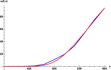
Figure 1: The graph of the measure based Black-Scholes solution (blue) versus the classical Black-Scholes solution (red).

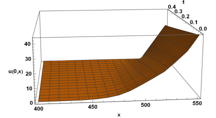
Figure 2: 3D representation of the measure based Black-Scholes solution.

To evaluate the adjustment quality of the measure based model, we plot the two models versus the scatter plot of the data:

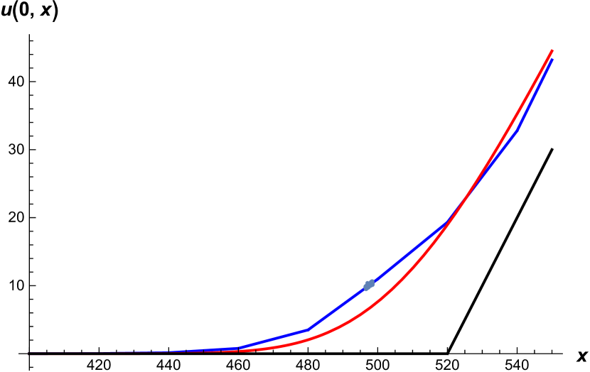
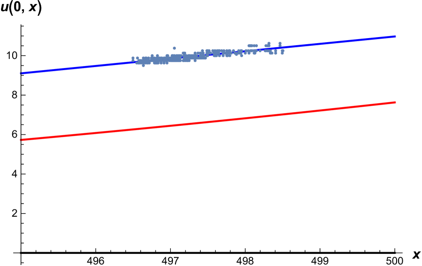
Figure 3: Fitted solution at different scales.

The measure based model offer a much better approximation of the solution, which can be measured by Tikhonov functional:

	Classical BS	Measure based BS
Tikhonov functional	$3375.05$	$4.49$

Table 2: Fit quality comparison.

We represent the parameters $\gamma_{i}/M$ in terms of a probability density function. To focus on those belonging to the data region, we will use an adaptive mesh:

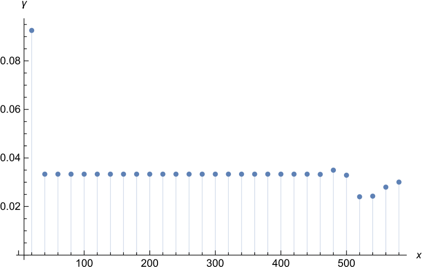
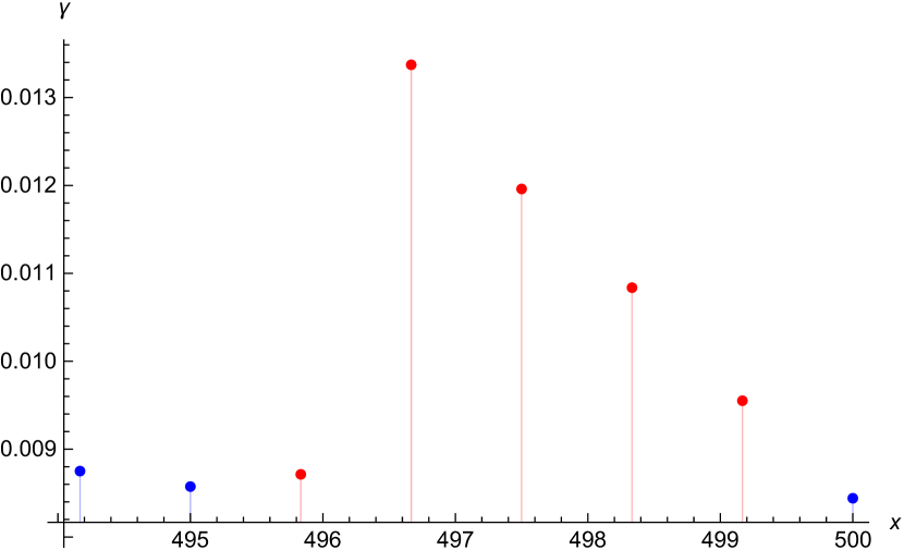
Figure 4: Parameters $\gamma_{i}/M$ of the probability measure.

We remark that the parameters grows up entering the data region before they start decreasing. A quick look at the solution dynamic equation, shows as that the $\gamma_{i}$ represent the market rigidity : higher is $\gamma_{i}$ more stable is the call price at the value $x_{i}$, we can see that the origin represent the most stable price (no one expect the price to vary there) and the region $[496.5,497]$ present more confidence in the market. Moreover, the parameters are much smaller than the classical model, except the origin, proving that the classical model represent an isotropic market with uniform uncertainty distribution.

5 Discussion

The results established in this work demonstrate the superiority of the measure based Black-Scholes model in term of market data fit, while the classical model underestimate the option price.

The measure based Black-scholes offer a new information on the market consisting in the measure $\mu$ which can be interpreted as a market confidence measure : by considering the probability version $\nu=\displaystyle\frac{\mu}{M}=\sum\frac{\gamma_{i}}{M}\,\delta_{i}$, the parameter $\gamma_{i}$ represent the option price rigidity at the stock price $x_{i}$, higher is $\gamma_{i}$ more stable is the option price.

One remarkable fact is the parameters for the estimated model are lower than the uniform case of the Black-Scholes model, reflecting more instability in the market than the classical theory predict.

The model based on the measure $\mu$ open a new field of research by quantifying the market confidence (in opposition with market incertitude) : $\gamma(x)$ reflect the market confidence at the stock price $x$, inducing more rigidity and a slow change in the option price. This is just a measure of incertitude in the market, which was considered to be unmeasurable.

References

• [All07] G. Allaire. Conception optimale de structures. Springer, 2007.
• [AP05] Y. Achdou and O. Pironneau. Computational Methods for Option Pricing. Society for Industrial and Applied Mathematics, 2005.
• [BP13] K. Bredies and H. K. Pikkarainen. Inverse problems in spaces of measures. ESAIM: Control, Optimisation and Calculus of Variations, 19:190–218, 2013.
• [Bre83] H. Brezis. Analyse fonctionnelle : théorie et applications. Éditions Masson, 1983.
• [BS73] F. Black and M. Scholes. The pricing of options and corporate liabilities. The Journal of Political Economy, 81:637–654, 1973.
• [GFS99] R. C. Stapleton G. Franke and M. G. Subrahmanyam. When are options overpriced? the black–scholes model and alternative characterisations of the pricing kernel. European Finance Review, 3:79–102, 1999.
• [LM68] J. L. Lions and E. Magenes. Problèmes aux limites non homogènes et applications. Dunod, 1968.
• [LMM05] G. C. Lim, G. M. Martin, and V. L. Martin. Parametric pricing of higher order moments in s&p500 options. Journal of Applied Econometrics, 20(3):377–404, 2005.
• [Mau07] Karin Mautner. Numerical treatment of the black-scholes variational inequality in computational finance. 2007.
• [RD19] N. Riane and C. David. The finite difference method for the heat equation on sierpiński simplices. International Journal of Computer Mathematics, 96(7):1477–1501, 2019.
• [RD20a] N. Riane and C. David. Sierpiński gasket versus arrowhead curve. Communications in Nonlinear Science and Numerical Simulation, 89:105311, 2020.
• [RD20b] N. Riane and Cl. David. Towards the self-similar Black-Scholes equation, 2020.
• [RD21a] N. Riane and C. David. The finite volume method on sierpiński simplices. Communications in Nonlinear Science and Numerical Simulation, 92:105468, 2021.
• [RD21b] N. Riane and Cl. David. An inverse Black-Scholes problem. Optimization and Engineering, 2021.
• [Zei90] E. Zeidler. Nonlinear functional analysis and its applications. II/A. : Linear monotone operators. Springer, 1990.