Magnetic fields inferred by Solar Orbiter: A comparison between SO/PHI-HRT and SDO/HMI

Abstract

Context. The High Resolution Telescope (HRT) of the Polarimetric and Helioseismic Imager on board the Solar Orbiter spacecraft (SO/PHI) and the Helioseismic and Magnetic Imager (HMI) on board the Solar Dynamics Observatory (SDO) both infer the photospheric magnetic field from polarised light images. SO/PHI is the first magnetograph to move out of the Sun–Earth line and will provide unprecedented access to the Sun’s poles. This provides excellent opportunities for new research wherein the magnetic field maps from both instruments are used simultaneously.

Aims. We aim to compare the magnetic field maps from these two instruments and discuss any possible differences between them.

Methods. We used data from both instruments obtained during Solar Orbiter’s inferior conjunction on 7 March 2022. The HRT data were additionally treated for geometric distortion and degraded to the same resolution as HMI. The HMI data were re-projected to correct for the $3^{\circ}$ separation between the two observatories.

Results. SO/PHI-HRT and HMI produce remarkably similar line-of-sight magnetograms, with a slope coefficient of $0.97$, an offset below $1\,$G, and a Pearson correlation coefficient of $0.97$. However, SO/PHI-HRT infers weaker line-of-sight fields for the strongest fields. As for the vector magnetic field, SO/PHI-HRT was compared to both the $720$-second and $90$-second HMI vector magnetic field: SO/PHI-HRT has a closer alignment with the $90$-second HMI vector. In the weak signal regime ($<600$ G), SO/PHI-HRT measures stronger and more horizontal fields than HMI, very likely due to the greater noise in the SO/PHI-HRT data. In the strong field regime ($\gtrsim 600$ G), HRT infers lower field strengths but with similar inclinations (a slope of $0.92$) and azimuths (a slope of $1.02$). The slope values are from the comparison with the HMI $90$-second vector. Possible reasons for the differences found between SO/PHI-HRT and HMI magnetic field parameters are discussed.

1 Introduction

The Solar Orbiter (see Müller et al. 2013, 2020) spacecraft was launched on 10 February 2020 and entered its Nominal Mission Phase in November 2021. The Polarimetric and Helioseismic Imager on the Solar Orbiter mission (SO/PHI; see Solanki et al. 2020) infers the photospheric magnetic field and line-of-sight (LoS) velocity from images of polarised light. It does this by sampling the Fe i $6173$ Å absorption line at five wavelength positions and an additional point in the nearby continuum. Differential imaging is performed to acquire the Stokes $(I,Q,U,V)$ vector. SO/PHI has two telescopes: the High Resolution Telescope (SO/PHI-HRT; Gandorfer et al. 2018) and the Full Disc Telescope. In this paper only data from SO/PHI-HRT are discussed.

Solar Orbiter has a highly elliptic orbit with a perihelion as small as $0.28$ au on some orbits. SO/PHI is the first magnetograph to move out of the Sun–Earth line. From 2025 on, with the help of Venus gravity assist manoeuvres, Solar Orbiter will reach heliolatitudes of $33^{\circ}$.

The Solar Dynamics Observatory (SDO; see Pesnell et al. 2011) was launched on 11 February 2010 and orbits the Earth in a circular geosynchronous orbit with a $28\degree$ inclination. Like Solar Orbiter, SDO carries a magnetograph: the Helioseismic Magnetic Imager (HMI; Scherrer et al. 2012; Schou et al. 2012). HMI has been in regular science operations since 1 May 2010. Similar to SO/PHI, it samples the $6173$ Å Fe i line at six points but at somewhat different wavelength positions.

Table 1: SO/PHI-HRT and SDO/HMI instrument specifications.

Specification	SO/PHI-HRT	SDO/HMI
Working wavelength	$6173$ Å	$6173$ Å
Wavelength positions	$-140,-70,0,70,140,$ $+$ or $-300$ mÅ	$-172,-103,34,34,103,172$ mÅ
Field of view	$0.28\degree\times 0.28\degree$	$0.57\degree\times 0.57\degree$
Aperture diameter	$140$ mm	$140$ mm
Spectral profile width	$106$ mÅ	$76$ mÅ
Detector size	$2048\times 2048$ pixels	$4096\times 4096$ pixels
Plate scale	$0.5$ ″	$0.5$ ″
Spatial resolution	$203$ km (0.28 au) - $725$ km (1.0 au)	$725$ km

The relevant technical details of SO/PHI-HRT and HMI are shown in Table 1. As can be seen, SO/PHI-HRT and HMI share some technical specifications: the same working wavelength, aperture diameter, and plate scale. It is important to know that, unlike SO/PHI, HMI has two identical cameras. One is dedicated to the LoS observables – the LoS magnetic field ($B_{\rm LOS}$) and the LoS velocity – and is referred to as the ‘front camera’. The second camera, known as the ‘side camera’, is used together with the front camera to capture the full Stokes vector, in order to retrieve the vector magnetic field.

With SO/PHI and HMI now operating simultaneously, they provide excellent opportunities for new research that combines data from both instruments. For example, stereoscopy is now possible, allowing for simultaneous observations of the same feature on the solar surface from two different viewpoints. This can be used to investigate the Wilson depression of sunspots (Romero Avila et al. 2023) and test disambiguation techniques for the magnetic field azimuth (Valori et al. 2022, 2023). These and many other applications build on the premise that the two instruments provide very similar measurements of the magnetic vector. Here we test this assumption and compare the magnetic fields inferred by SO/PHI-HRT and HMI and try to understand their similarities and differences.

In Sect. 2 the data from both instruments used in this study and their properties are presented. In Sect. 3 the detailed method for this comparison is given. The results of the comparison of the magnetic field data products from SO/PHI-HRT and HMI are discussed in Sect. 4, and in Sect. 5 we outline the conclusions reached from this work.

2 Data

The data used in this study are from 7 March 2022 (see Table 2) and thus from around Solar Orbiter’s inferior conjunction – that is, when Solar Orbiter was on the Sun–Earth line – which took place at 09:01:56 UTC (Coordinated Universal Time) on 7 March 2022. Solar Orbiter’s elevation from the ecliptic plane was $2.949^{\circ}$ at inferior conjunction, and the effective angular separation between the two spacecraft during the observation period ranged from $3.006^{\circ}$ to $3.024^{\circ}$. During this time, Solar Orbiter was at a distance to the Sun of between 0.493 au and 0.501 au. On the photosphere, the nominal spatial resolution of SO/PHI-HRT at this distance is $363$ km. In the common field of view (FoV) was a sunspot with negative polarity located at a heliocentric angle of $\mu=\cos\theta=0.87$ as seen by SO/PHI-HRT.

2.1 SO/PHI-HRT magnetic field

The SO/PHI-HRT data were collected to support a nanoflare and active region Solar Orbiter Observing Plan (see Zouganelis et al. 2020). The raw data from this observation campaign were downlinked to Earth and processed using the on-ground data reduction and calibration pipeline (Sinjan et al. 2022). In addition, the data were processed to remove residual wavefront errors, which originate mostly from the telescope’s entrance window. This was achieved using a point spread function (PSF) determined from phase diversity analysis (Paxman et al. 1992; Löfdahl & Scharmer 1994). Additionally, in the same processing step as the PSF deconvolution, a convolution with the instrument’s theoretical Airy disc was performed. This produced data without optical aberrations, with increased contrast, and limited the noise that would otherwise be added by the deconvolution procedure. For further information regarding phase diversity analysis and the SO/PHI-HRT PSF, we refer the reader to Kahil et al. (2022, 2023). To determine the magnetic field vector, the radiative transfer equation (RTE) was inverted with C-MILOS (Orozco Suárez & Del Toro Iniesta 2007) in the full vector mode, which assumes a Milne-Eddington (ME) atmosphere and uses classical estimates (CE) as the initial conditions for the inversion (Semel 1967; Rees & Semel 1979; Landi Degl’Innocenti & Landolfi 2004). For operational reasons, SO/PHI-HRT’s Image Stabilisation System (ISS) was switched off. The SO/PHI-HRT LoS magnetograms used in this study were generated from the vector magnetic field obtained from the RTE inversion: $B_{\rm LOS}=B\,\cos\gamma$, where $B_{\rm LOS}$ is the LoS component of the magnetic field, $B$ is the field strength, and $\gamma$ is the angle of the field to the LOS.

The data from this campaign were recorded with a $60$-second cadence. As shown in Sinjan et al. (2022), this mode results in quiet-Sun magnetograms with a noise of $8.3$ G (with ISS on). Future investigations, using data planned to be gathered during Solar Orbiter’s next inferior conjunction in March 2023, will attempt to quantify the impact of non-ISS operation on the comparison.

Table 2: Observation details of used SO/PHI-HRT and HMI data.

	SO/PHI-HRT	SDO/HMI
Start time	2022-03-07 00:00:09 UTC	2022-03-07 00:00:00 TAI
End time	2022-03-07 01:06:09 UTC	2022-03-07 01:12:00 TAI
Distance	$0.493-0.501$ au	$0.992$ au
ISS mode	Off	On
Processing	Ground	Ground
RTE mode	C-MILOS: CE+RTE	VFISV
	Vector	Line of sight		Vector
Cadence	$60$ s	$45$ s	$720$ s	$90$ s	$720$ s
Number of datasets	$56$	$56$	$7$	$38$	$7$

2.2 HMI magnetic field

HMI treats its LoS and vector data products separately, each having two options for observing cadence. For this comparison study, all four possible data products were compared with SO/PHI-HRT (see Table 2). The vector data products were generated from the HMI vector pipeline (Hoeksema et al. 2014), while the LoS products were generated with an algorithm similar to that used by the Michelson Doppler Imager (MDI) on board the Solar & Heliospheric Observatory, hereafter referred to as the MDI-like algorithm (Couvidat et al. 2012). The HMI LoS versus HMI vector has been compared by Hoeksema et al. (2014), who show that the MDI-like algorithm underestimates the field strength in the strong field regime ($\left|B_{\rm LOS}\right|>600$ G) compared to the inversion result. The HMI $45$-second and $720$-second LoS magnetograms have a noise level in the quiet Sun, near disc centre, of $7-9$ G and $3-4$ G, respectively (Couvidat et al. 2016; Liu et al. 2012).

The $45$-second magnetograms are produced every $45$ seconds from an interpolation of Stokes $I+V$ and Stokes $I-V$ filtergrams from a $270$-second interval (Liu et al. 2012; Couvidat et al. 2016). Since 13 April 2016, the full Stokes vector has been captured at a $90$-second cadence and inverted to create the vector magnetic field data product. This cadence is achieved by combining images from both cameras (Liu et al. 2016). To produce the $720$-second vector data product, a weighted temporal average is made every $720$ seconds, combining $90$-second Stokes vector maps collected over a period of more than $20$ minutes and inverted using the very fast inversion of the Stokes vector (VFISV) ME code (Hoeksema et al. 2014; Borrero et al. 2011). In Sect. 3 we describe the method by which we take the difference in interval and light travel time into account to ensure co-temporal observations are compared.

3 Method

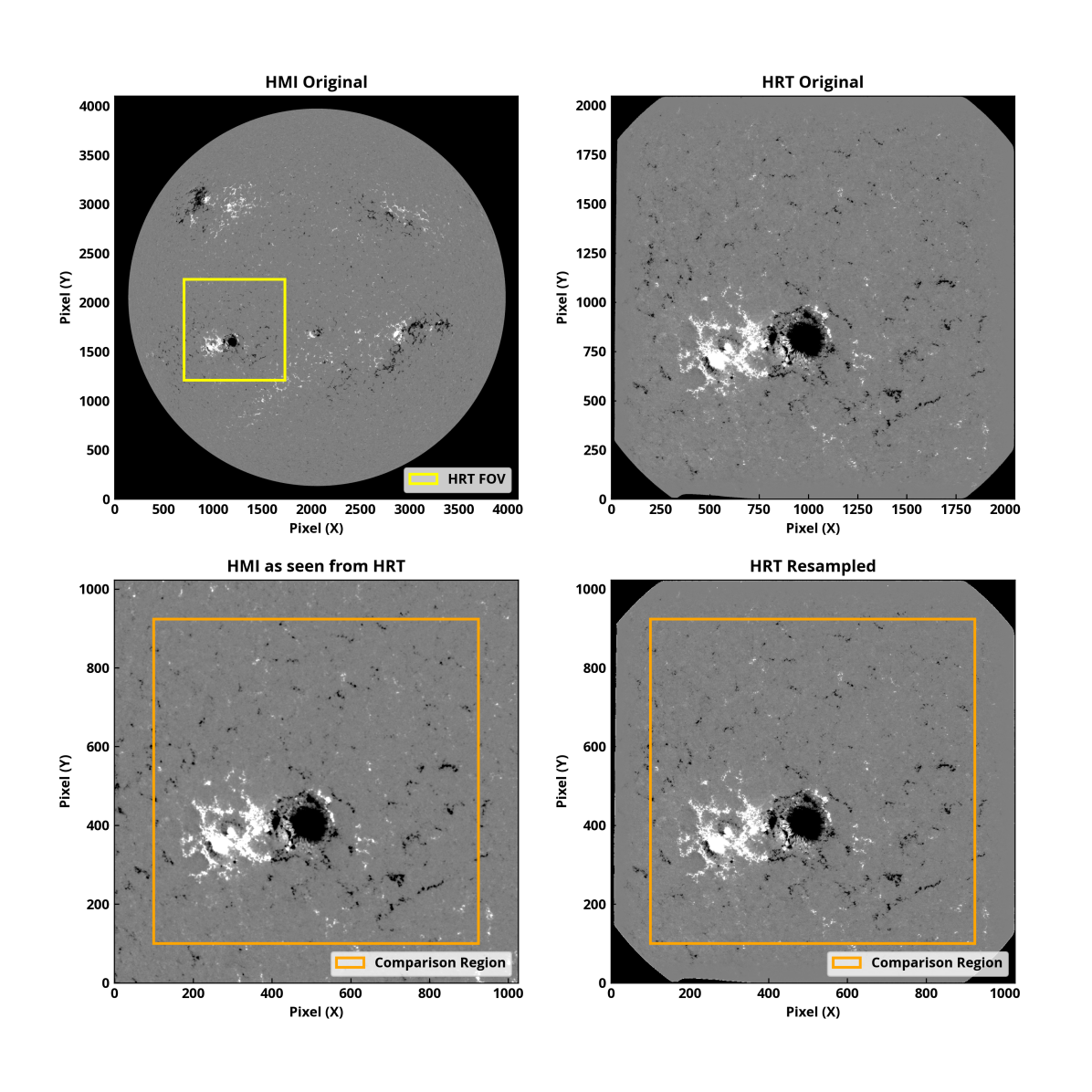
Figure 1: Magnetograms from HMI and SO/PHI-HRT on 7 March 2022. Top left: HMI $45$-second LoS magnetogram at 00:01:30 TAI, with the SO/PHI-HRT FoV shown in yellow. The pixels outside the solar disc are set to black for clarity. Top right: SO/PHI-HRT $60$-second magnetogram at 00:00:09 UTC. The pixels outside the field stop are set to black for clarity. Bottom left: Sub-region of the HMI magnetogram from the top-left panel, which has been re-projected to the SO/PHI-HRT frame of reference. Bottom right: SO/PHI-HRT magnetogram resampled to HMI resolution. The orange square outlines the regions used for the comparison. All magnetograms are saturated at $\pm 200\,$G.

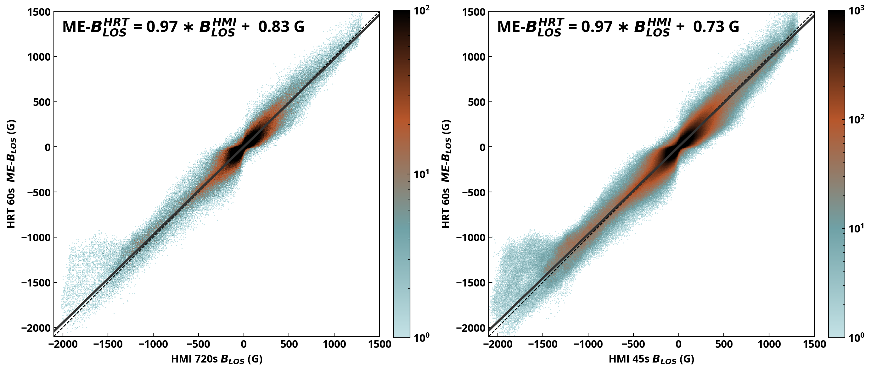
Figure 2: Scatter plot comparing pairs of SO/PHI-HRT $60$-second ME-$B_{\rm LOS}$ and HMI $B_{\rm LOS}$. The log density of the pixels is shown and saturated at 100 (a) and 1000 (b) pixels per plotted point for clarity. The averaged linear fit (of HMI vs SO/PHI-HRT and SO/PHI-HRT vs HMI) is shown with the solid grey line, and a one-to-one correspondence is indicated by the dashed black line. Panel (a): Seven pairs with HMI $720$-second magnetograms. Panel (b): $56$ pairs with HMI $45$-second magnetograms. See the main text for a more detailed description.

We compared the magnetic field inferred by SO/PHI-HRT and HMI on a pixel-to-pixel basis. The HMI data were corrected for geometric distortion across the camera (Hoeksema et al. 2014), and the SO/PHI-HRT data were corrected using a preliminary distortion model, derived from calibration data pre-launch. The method we now describe has been applied to each comparison of the individual data products. We provide here an example for one pair of LoS magnetograms: First a SO/PHI-HRT $60$-second magnetogram was selected and the closest HMI $45$-second magnetogram in time was found (see the top panels in Fig. 1). This was done by comparing the average time of the observations, taking into account the different distances of Solar Orbiter and SDO from the Sun, and hence the different light travel times, as well as the difference between TAI (International Atomic Time) and UTC time. Secondly, the sub-region of the HMI FoV common to both telescopes, outlined in yellow in Fig. 1, was re-projected using the DeForest (2004) algorithm onto the SO/PHI-HRT detector frame of reference using the World Coordinate System (WCS) information (Thompson 2006).

Next, the SO/PHI-HRT data were resampled using linear interpolation to match the factor of two lower spatial resolution of the HMI data (SO/PHI-HRT was half the distance to the Sun at the time of observation). Applying boxcar binning or cubic interpolation makes no significant difference to the results of the comparison. As both SO/PHI-HRT and HMI have the same aperture diameter, their PSFs are similar. However, by resampling SO/PHI-HRT we change the effective PSF. The impact of this effect is left for future studies. Residual rotation and translation perpendicular to the normal of the SO/PHI-HRT image plane were found using a log-polar transform (cf. e.g. Sarvaiya et al. 2009) and corrected. The result of such corrections is shown in the bottom panels of Fig. 1. These corrections are due to inaccuracies in the WCS information. This process was repeated for each SO/PHI-HRT magnetogram.

Finally, the maps were cropped by $100$ pixels at each side before the comparison was made, as outlined in orange in the lower panels of Fig. 1. This is because of the SO/PHI-HRT field stop, visible as the black region in Fig. 1, and because of the processing step to correct for residual wavefront errors. Within this procedure the image is apodised before the Fourier transform to ensure periodic boundaries, and the first $100$ pixels at each side were affected. These regions therefore had to be excluded from the comparison with HMI.

For comparison with the HMI $720$-second data products, a single SO/PHI-HRT dataset, the one closest to the average time of the HMI $720$-second dataset, was used. This comparison was performed for the LoS magnetic field component, $B_{\rm LOS}$, the magnetic field strength, $\left|\mbox{\boldmath$B$\unboldmath}\right|$, the inclination, $\gamma$, and the azimuth, $\phi$. Extra treatment was taken for the azimuth comparison: both HMI and SO/PHI-HRT define the azimuth anti-clockwise from the positive direction of the $y$-axis (Sinjan et al. 2022). After the re-projection of HMI, care was taken to ensure that both datasets used the same definition of the azimuth by taking the roll angle of each spacecraft into account.

4 Comparison of SO/PHI-HRT and HMI magnetic field observations

4.1 Comparison of SO/PHI-HRT and HMI LoS magnetograms

We stress here for clarity that, when discussing the LoS magnetograms from HMI, we refer to the LoS magnetic field derived using the MDI-like algorithm, referred to as $B_{\rm LOS}$. However, the magnetograms from SO/PHI-HRT presented here are the LoS component of the full vector magnetic field (determined by RTE inversion): we refer to this as ME-$B_{\rm LOS}$.

The scatter plot comparing the SO/PHI-HRT 60-second and HMI 720-second magnetograms is shown in Fig. 2a, where the logarithmic density of the points is indicated by the colour. This figure displays seven pairs of magnetograms; each of the SO/PHI-HRT 60-second magnetograms is recorded in the middle of the interval of time over which the HMI 720-second magnetogram that it is compared with is recorded. The solid black line is a linear fit to the distribution, which is the average of two linear fits, one of HMI versus SO/PHI-HRT and the other of SO/PHI-HRT versus HMI. This averaging removes statistical bias. As indicated by the fit, there is an excellent agreement between the two telescopes, with a slope value of $0.97$ and an offset of $0.83$ G. This offset could be an artefact of there being more very strong fields with negative polarity than with positive. The offset of the weak fields inferred by SO/PHI-HRT can be determined by histogram analysis: Sinjan et al. (2022) demonstrate that the SO/PHI-HRT $B_{LOS}$ distribution in the quiet Sun is centred near zero with an offset of $-0.18$ G. The Pearson correlation coefficient is $0.97$. The linear fit, absolute error on the slope and offset, and Pearson correlation coefficient (cc) are shown in Table 3 for all compared quantities presented in this paper. In the case of Fig. 2, the errors on the slope and offset are negligible.

However, a difference is present for the strongest fields. We selected pixels where HMI $720$-second $B_{\rm LOS}<-1300$ G, the point at which a large divergence between SO/PHI-HRT and HMI appears. The mean difference between them is $+149\pm 2$ G relative to the (negative) HMI values, which corresponds to $9$% weaker LoS fields relative to HMI. The error here denotes the standard error in the mean; the scatter ($1\sigma$) of the distribution of absolute differences is $197$ G. The pixel selection threshold (HMI $720$-second $B_{\rm LOS}<-1300$ G) corresponds to pixels only in the leading sunspot in the FoV, where $81$ % are in the umbra and the remaining $19$ % in the penumbra. The umbra and penumbra classification was determined using $I_{c}<0.55$ and $0.55I_{c}<0.95$ thresholds on the SO/PHI-HRT continuum intensity, $I_{c}$; these thresholds are the same as those used in Dalda (2017), where the magnetic field between HMI and Hinode/SP is compared. It must also be noted that the distribution in Fig. 2 is not symmetric between fields of opposite polarity. This is because no strong fields above $1350$ G were observed in HMI in the common FoV, while SO/PHI-HRT infers fields of up to $1500\,$G. Under similar conditions, we expect the comparison between the two telescopes in the positive strong field regime to be similar to that observed in the negative strong field regime, with SO/PHI-HRT measuring lower LoS field components compared to HMI.

The comparison with HMI $45$-second magnetograms (Fig. 2b), where $56$ pairs of data were compared, reveals very similar results. This was expected as the $45$-second and $720$-second HMI magnetograms are well inter-calibrated (Liu et al. 2012). For pixels where the HMI $45$-second $B_{\rm LOS}<-1300$ G, there is a similar mean difference of $+155.5\pm 0.9$ G relative to the (negative) HMI values, which again corresponds to $9\%$ weaker LoS magnetic fields inferred by SO/PHI-HRT in this regime.

In both Fig. 2a and b, all pixels are plotted, including those with signal below the noise. There is an hourglass shape around the origin present in both panels. This could be due to a mismatch in the alignment of the sets of magnetograms. As described in Sect. 3, we applied only a preliminary model to correct for geometric distortion in SO/PHI-HRT, which could explain inaccuracies in the alignment.

There are several effects that could explain the difference between SO/PHI-HRT and HMI for the strongest fields. Firstly, the two instruments use different methods to infer the LoS magnetic field: HMI uses the MDI-like formula, while SO/PHI-HRT uses a radiative transfer code. Additionally, the two instruments sample the Fe i line at different positions, and SO/PHI-HRT observes farther out in the continuum ($\pm 300$ mÅ from the line core vs $\pm 172$ mÅ for HMI). For the strongest fields, the very large Zeeman splitting results in the two instruments capturing different information from the true Stokes signal, which is then interpreted by the inversion routines differently. A detailed investigation of these effects is beyond the scope of this paper. Furthermore, the spectral profile width is different: SO/PHI-HRT has a full width half maximum (FWHM) of $106$ mÅ, while the FWHM of HMI is $76$ mÅ. There could also be a contribution from stray light, in particular for the pixels in the umbra, as neither HMI nor SO/PHI-HRT are corrected for stray light in their standard data pipelines.

Finally, it is known that HMI suffers from a 24-hour periodicity (Liu et al. 2012; Hoeksema et al. 2014; Couvidat et al. 2016) in its magnetic field observables due to the SDO orbit. The velocity relative to the Sun oscillates by $\pm 3.5$ km/s on a 24-hour period, with further variation of hundreds of metres per second due to Earth’s orbit. The SDO solar radial velocity for the data considered in this study started at $3.249\,$km/s and ended at $3.291\,$;m/s. Couvidat et al. (2016) show that the $B_{\rm LOS}$, calculated using the MDI-like algorithm, in the umbra depends quadratically on the magnitude of the velocity. A residual of between $+50$ G and $+100$ G was present when SDO had a radial velocity near $\pm 3\,$km/s. This residual is the value once the long-term variations ($\geq 2$ day) are removed. It explains approximately half of the observed difference in the strong signal regime. It is plausible, although not certain, that, when combined with the effects from the different wavelength sampling, different inversion codes, and stray light, it explains the observed discrepancy.

4.2 Comparison of SO/PHI-HRT and HMI vector magnetic fields

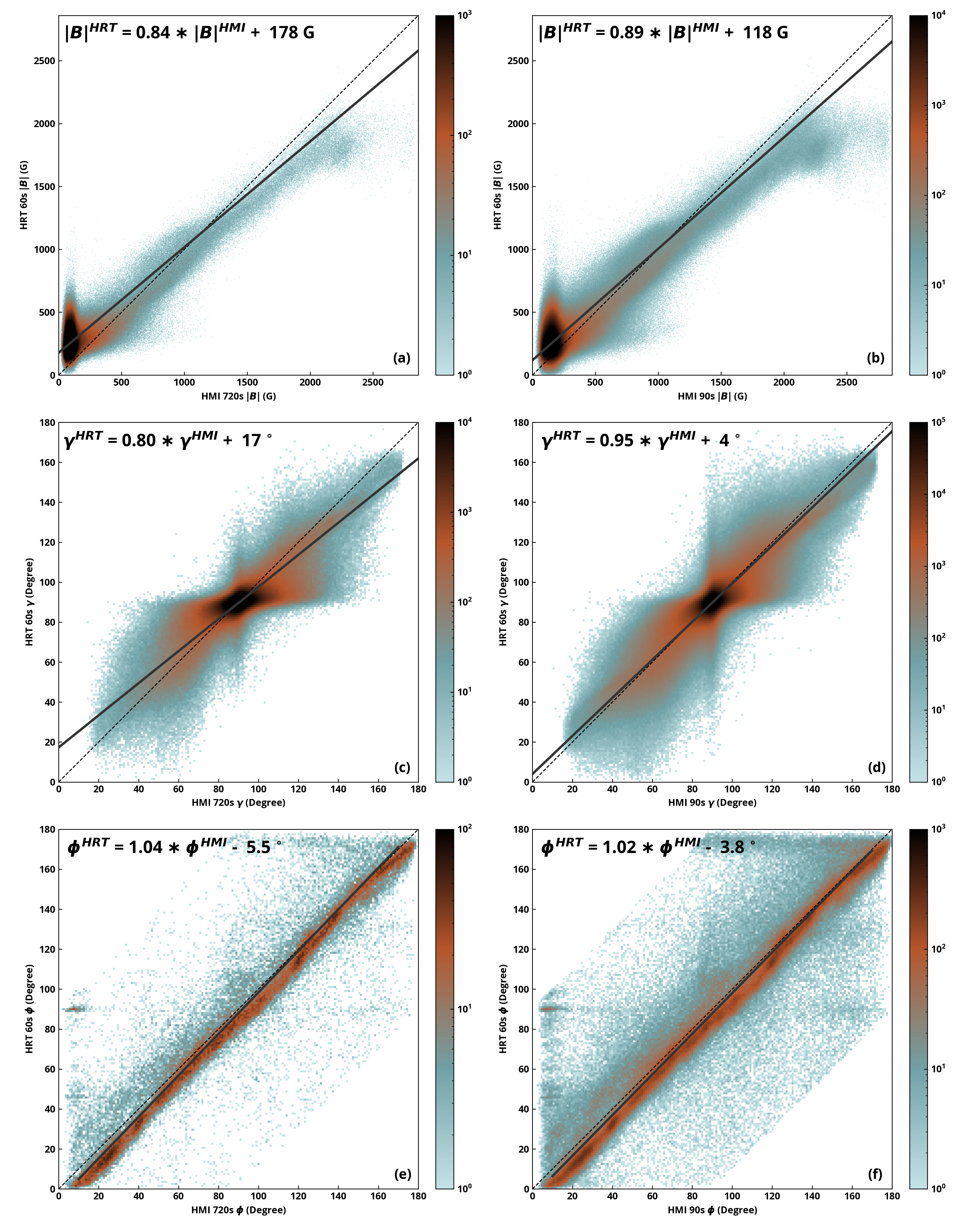
Figure 3: Scatter plots comparing SO/PHI-HRT and HMI vector magnetic field maps. The first column compares inversion results from seven pairs of SO/PHI-HRT $60$-second and HMI $720$-second datasets, while the second column does the same for $38$ pairs of SO/PHI-HRT $60$-second and HMI $90$-second datasets. The log density of the pixels is given by the colour scale and is saturated for clarity. The averaged linear fit and $y=x$ are given by the solid grey and dashed black lines, respectively. Panels (a) and (b): Magnetic field strength. Panels (c) and (d): Magnetic field inclination (relative to the LoS). Panels (e) and (f): Magnetic field azimuth. Pixels where $|\phi_{\text{HMI}}-\phi_{\text{HRT}}|>90\,\degree$ and $\mathbf{\left|B\right|}_{HRT}<600\,$G are omitted and not included in the fit.

Here we compare the SO/PHI-HRT and HMI vector magnetic fields, both inferred by RTE inversions of the Stokes vector albeit using different inversion codes. We would like to highlight the $3^{\circ}$ angular separation between SO/PHI-HRT and HMI, mentioned in Sect. 2. This has no impact on $\mathbf{\left|B\right|}$, and from a simple rotation test on SO/PHI-HRT data, we estimate that it does not significantly impact the magnetic field inclination or azimuth, except for producing an offset of a few degrees in the azimuth.

First we compared the magnetic field strengths, $\mathbf{\left|B\right|}$, as shown in the top row of Fig. 3. Both SO/PHI-HRT and HMI assume a magnetic filling factor of unity for the RTE inversion, so the field strength is averaged over the pixel. Consequently, we do not distinguish between magnetic field strength and magnetic flux density, as is sometimes done in the literature. In Fig. 3a the comparison between the SO/PHI-HRT and HMI $720$-second $\mathbf{\left|B\right|}$ is depicted, while in Fig. 3b the comparison with the HMI $90$-second $\mathbf{\left|B\right|}$ is shown. The slope is $0.84$ and $0.89$ in Fig. 3a and b, respectively. The higher slope value for the $90$-second comparison is because the variance is more similar to that of the SO/PHI-HRT data than for the HMI $720$-second data. The magnetic field strengths of the two instruments have a correlation coefficient of $0.85$ and $0.84$ for the $720$-second and $90$-second $\mathbf{\left|B\right|}^{HMI}$, respectively.

We observe here that in the weaker field regime, SO/PHI-HRT infers stronger fields. Following Liu et al. (2012), we arbitrarily used a boundary value of $600$ G to define the weak signal regime. In this regime there is a dense distribution of pixels, seen in both Fig. 3a and b, which we refer to as the ‘hot zone’, that portrays a discrepancy between the two instruments. The offset is mainly due to this hot zone, with an offset of $178$ G in Fig. 3a and a lower offset of $118$ G in Fig. 3b. The difference in the offset perhaps reflects the noise difference between the $90$-second and $720$-second $\mathbf{\left|B\right|}^{HMI}$. The hot zone in Fig. 3b has a larger extent for HMI compared to that in Fig. 3a, which may be due to the difference in noise level. Borrero & Kobel (2011) have demonstrated that Stokes profiles with higher noise levels, when inverted, result in stronger but more inclined fields. We note the more horizontal dense field central patches in Fig. 3c, Fig. 3d, and Fig. 4a. The higher noise level in SO/PHI-HRT compared to HMI is due to the ISS non-operation and, crucially, the longer averaging time within the HMI data. Furthermore, the deconvolution of part of the PSF also increased the noise of the SO/PHI-HRT data by $20$% (Kahil et al. 2023). Therefore, the noise levels of the original Stokes vector in SO/PHI-HRT are $1.8\times 10^{-3},\,2.2\times 10^{-3}$, and $\,1.8\times 10^{-3}$ for $Q/I_{c}$, $U/I_{c}$, and $V/I_{c}$, respectively, where $I_{c}$ denotes Stokes $I$ in the continuum. In comparison, the noise in the HMI $720$-second Stokes vector is $9\times 10^{-4}$ for $Q/I_{c}$, $U/I_{c}$, and $V/I_{c}$, (Couvidat et al. 2016). The noise in the $90$-second Stokes vector, however, has not been quantified in the literature because this is a non-standard data product.

Now we turn to the strong signal regime in Fig. 3a and b. At approximately $\mathbf{\left|B\right|}\,>1300$ G for both HMI and SO/PHI-HRT,  the distribution starts diverging from the $y=x$ line. For pixels where the fields in HMI are stronger than this value, SO/PHI-HRT infers a lower field strength. The field strength threshold of $1300$ G in HMI and SO/PHI-HRT corresponds to pixels where $38.1$ % are in the umbra, $61.4$ % are in the penumbra, and $0.5$ % lie elsewhere. For fields stronger than $1300$ G in SO/PHI-HRT or HMI, the mean difference between them was $-247\pm 1$ G and $-246.8\pm 0.4$ G relative to the HMI  for the HMI $720$-second and $90$-second comparisons, respectively ($\approx 13$% smaller relative to the HMI values in both cases). The error on the mean is the standard error. The scatter ($1\sigma$) of the distribution of the differences is roughly $180$ G in both cases, highlighting the large width of these distributions. While we cannot directly compare these mean differences to those presented in Sect. 4.1, because the strong magnetic field lines are not all along the LoS and we consider more pixels in the penumbra, we can still qualitatively deduce that we observe a larger separation between HMI and SO/PHI-HRT for the magnetic field strength. Important to note is that in Fig. 2 we compare the ME-$B_{LOS}^{HRT}$, which was derived from the full vector, while the $B_{LOS}^{HMI}$ in Fig. 2 was calculated using the MDI-like formula. In Sect. 4.3 the LoS components derived from the full vectors are compared.

The inclination of the magnetic vector, $\gamma$, relative to the LoS, as deduced from the two instruments, is compared in the second row of Fig. 3. The slope is $0.80$ and $0.95$ for the HMI $720$-second and $90$-second comparisons, respectively. The correlation coefficient between SO/PHI-HRT and the HMI $720$-second and $90$-second magnetic field inclination is $0.81$ and $0.85,$ respectively. It is clear that both instruments agree on the polarity of the magnetic field relatively well (there is a dearth of points in the upper-left and lower-right quadrants of Fig. 3c and d). We also note here that HMI has a somewhat stronger tendency to infer inclinations close to $90\,^{\circ}$ (the vertical streak at $90\,^{\circ}$ is stronger than the horizontal one). The biggest difference between the inclinations inferred by the two instruments is, however, that SO/PHI-HRT data result in somewhat more horizontal fields (the slope of the solid black lines in Fig. 3c and d is less than unity). There is a closer agreement in Fig. 3d, with a slope of $0.95$, as the variance in the HMI $90$-second data is closer to the SO/PHI-HRT variance. The offsets shown in both Fig. 3c and d are not relevant here as the point of symmetry lies at ($90^{\circ},90^{\circ}$). The averaged linear fit crosses ($90^{\circ},90^{\circ}$) with an offset of less than half a degree in both Fig. 3c and d. From the simple rotation test on SO/PHI-HRT data mentioned earlier, the $3^{\circ}$ angular separation between SO/PHI-HRT and HMI could introduce an offset of $<1^{\circ}$. Furthermore, a small part of the scatter – the distance of the points from the line of best fit – is likely due to the $3^{\circ}$ difference in view direction.

In Fig. 4 we compare the inclination for the weak and strong field cases. In Fig. 4a pixels are shown where $\mathbf{\left|B\right|}_{\text{HRT}}<600$ G or $\mathbf{\left|B\right|}_{\text{HMI}}<600$ G, while in Fig. 4b pixels are shown where $\mathbf{\left|B\right|}_{\text{HRT}}>600$ G and $\mathbf{\left|B\right|}_{\text{HMI}}>600$ G. In Fig. 4b the distribution of the points is much closer to the line of best fit, with a correlation coefficient of $0.98$, compared to a correlation coefficient of $0.80$ in Fig. 4a. The slope in Fig. 4b, however, is slightly lower than that in Fig. 4a.

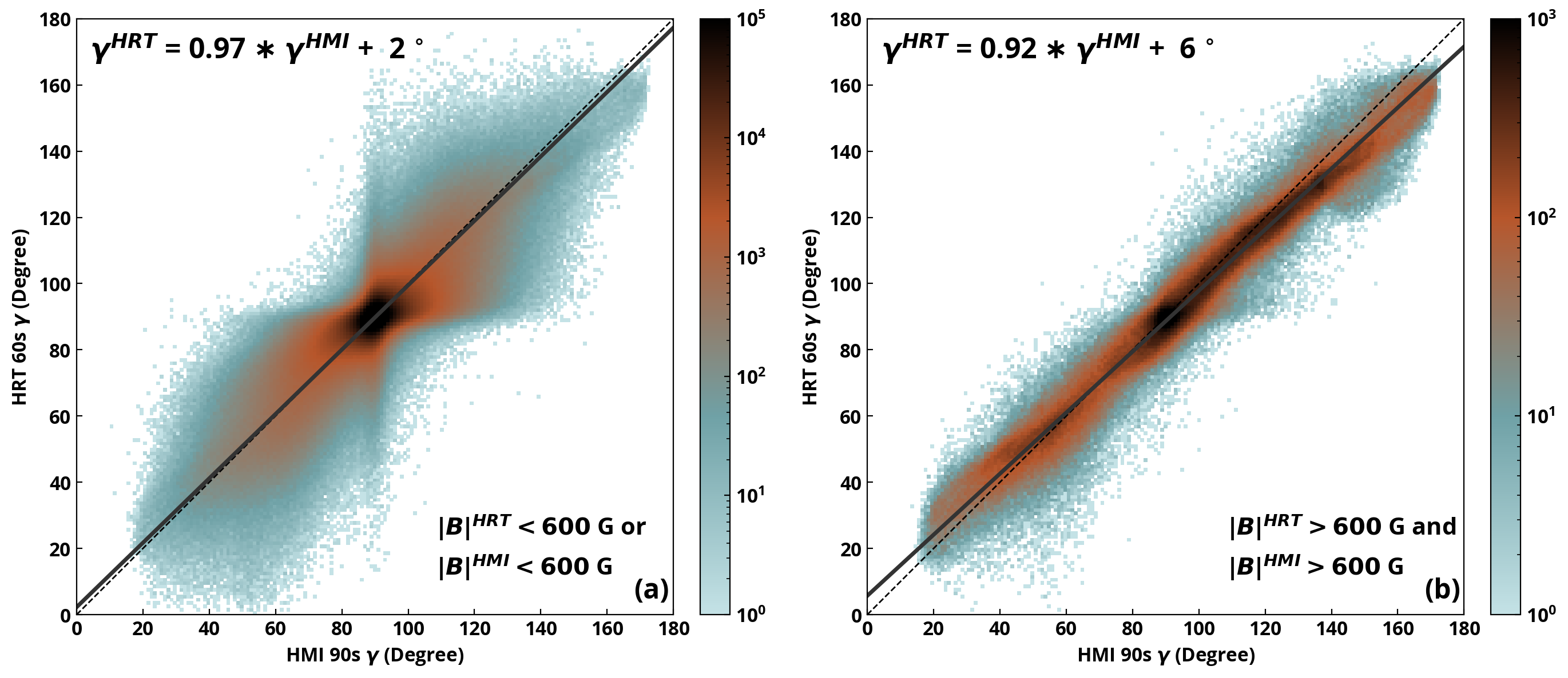
Figure 4: Scatter plots comparing SO/PHI-HRT $60$-second and HMI $90$-second magnetic field inclination. Panel (a): Pixels where $\mathbf{\left|B\right|}_{\text{HRT}}<600$ G or $\mathbf{\left|B\right|}_{\text{HMI}}<600$ G. Panel (b): Pixels where $\mathbf{\left|B\right|}_{\text{HRT}}>600$ G and $\mathbf{\left|B\right|}_{\text{HMI}}>600$ G. The log density of the pixels is shown and is saturated for clarity. The averaged linear fit and $y=x$ are shown with the solid grey and dashed black line, respectively.

The comparison of the azimuth, $\phi$, is shown in the bottom row of Fig. 3. For this comparison, only pixels from and around the leading sunspot in the FoV, with $B_{\text{HRT}}>600\,$G, were selected. Furthermore, for the linear fit, pixels where $|\phi_{\text{HMI}}-\phi_{\text{HRT}}|>90\,\degree$ were not considered as they are affected by the intrinsic $180\,\degree$ ambiguity of the azimuth. Finally, the regions near $0\,\degree$ and $180\,\degree$ were excluded from the linear fits to avoid an artificial shift, as the end points were not periodic. There are strong correlation coefficients of $0.95$ and $0.94$ (HMI $720$-second and $90$-second comparisons, respectively). One reason why there is a strong correlation is that the HMI transverse magnetic field does not suffer from the $12-$ or $24$-hour periodicity due to the SDO orbit (Hoeksema et al. 2014). As shown in Fig. 3e and f, the slope is $1.04$ and $1.02,$ respectively, implying that SO/PHI-HRT infers azimuth angles slightly larger than that of HMI. There is also a negative, non-uniform offset of $-5.5\,^{\circ}$ in the $720$-second case, which is only $-3.8\,^{\circ}$ in the $90$-second case; this requires further investigation. The absolute errors on these offset values are $0.7$ and $1.7$, which are large relative to the computed offsets, as fewer points are considered relative to the other comparisons presented in this work. Were there an incorrect alignment of the $+y$ detector between SO/PHI-HRT and HMI,  which both define $\phi=0$, an offset between $\phi_{HMI}$ and $\phi_{HRT}$ would exist. To the best of our knowledge, we have aligned the $+y$ detector of both to solar north and thus rule this out as an origin of the observed offset. However, our rotation test also revealed that a rotation around axes orthogonal to the $+y$ detector axis could also result in an offset of $0^{\circ}$-$2^{\circ}$. Therefore, a part of the offset shown in Fig. 3 could originate from the angular separation between SO/PHI-HRT and HMI. In this test, the slope of the linear fit between the rotated and original SO/PHI-HRT, $\phi$, was $1.01$, a change of $1\%$, which is reflected in the slope error for the $\phi$ comparisons in Table 3. Additionally, a small part of the scatter may be due to the $3^{\circ}$ angular separation.

Something that could explain the discrepancies seen in all three components of the magnetic vector is the different wavelength sampling and spectral resolution, as mentioned in Sect. 4.1. This, combined with the use of different inversion routines (VFISV applied to HMI data and C-MILOS to SO/PHI-HRT data), is certain to result in differences between the two instruments. As mentioned in the discussion of the weak magnetic field strength regime, the difference in noise levels, in part due to longer HMI integration times, is the reason for the different inferred fields. A non-perfect alignment of the data, as mentioned in Sect. 4.1, could also be a factor in explaining the noted difference.

4.3 Comparison of SO/PHI-HRT and HMI LoS components of the full vector magnetic field

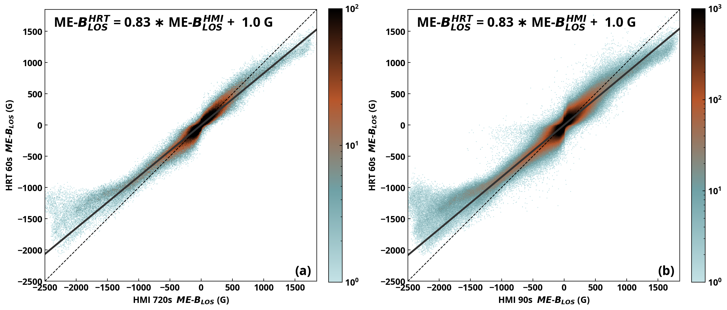
Figure 5: Scatter plots comparing the SO/PHI-HRT and HMI LoS components of the full vector magnetic field. ‘ME’ stands for Milne-Eddington and indicates that it is derived from RTE inversions. Panel (a): Comparison of inclinations from seven pairs of SO/PHI-HRT $60$-second and HMI $720$-second data. Panel (b): Same, but for $38$ pairs of SO/PHI-HRT $60$-second and HMI $90$-second data. The log density of the pixels is shown by the colour and is saturated at 1000 (panel a) and 100 (panel b) for clarity. The averaged linear fit and $y=x$ lines are plotted in solid grey and dashed black lines, respectively.

Table 3: Quantities compared, their linear fit, absolute errors on the slope and offset, and Pearson correlation coefficient (cc).

Quantities compared	Linear fit	Slope error	Offset error	Pearson cc
ME-$B_{LOS}^{HRT}$ $60$ s vs $B_{LOS}^{HMI}$ $720$ s	ME-$B_{LOS}^{HRT}=0.97\ast B_{LOS}^{HMI}+0.83$ G	$9\times 10^{-5}$	$0.01$	0.97
ME-$B_{LOS}^{HRT}$ $60$ s vs $B_{LOS}^{HMI}$ $45$ s	ME-$B_{LOS}^{HRT}=0.97\ast B_{LOS}^{HMI}+0.73$ G	$3\times 10^{-5}$	$0.006$	0.97
$\mathbf{\left|B\right|}^{HRT}$ $60$ s vs $\mathbf{\left|B\right|}^{HMI}$ $720$ s	$\mathbf{\left|B\right|}^{HRT}=0.84\ast\mathbf{\left|B\right|}^{HMI}+178$ G	$3\times 10^{-4}$	$0.02$	$0.85$
$\mathbf{\left|B\right|}^{HRT}$ $60$ s vs $\mathbf{\left|B\right|}^{HMI}$ $90$ s	$\mathbf{\left|B\right|}^{HRT}=0.89\ast\mathbf{\left|B\right|}^{HMI}+118$ G	$1\times 10^{-4}$	$0.01$	$0.84$
$\gamma^{HRT}$ $60$ s vs $\gamma^{HMI}$ $720$ s	$\gamma^{HRT}=0.80\ast\gamma^{HMI}+17\,^{\circ}$	$4\times 10^{-4}$	$0.01$	$0.81$
$\gamma^{HRT}$ $60$ s vs $\gamma^{HMI}$ $90$ s	$\gamma^{HRT}=0.95\ast\gamma^{HMI}+4\,^{\circ}$	$1\times 10^{-4}$	$0.004$	$0.85$
$\phi^{HRT}$ $60$ s vs $\phi^{HMI}$ $720$ s	$\phi^{HRT}=1.04\ast\phi^{HMI}-5.5\,^{\circ}$	$0.01$	$0.7$	$0.95$
$\phi^{HRT}$ $60$ s vs $\phi^{HMI}$ $90$ s	$\phi^{HRT}=1.02\ast\phi^{HMI}-3.8\,^{\circ}$	$0.01$	$1.7$	$0.94$
$\gamma^{HRT}$ $60$ s vs $\gamma^{HMI}$ $90$ s (weak-field)	$\gamma^{HRT}=0.97\ast\gamma^{HMI}+2\,^{\circ}$	$1\times 10^{-4}$	$0.006$	$0.80$
$\gamma^{HRT}$ $60$ s vs $\gamma^{HMI}$ $90$ s (strong-field)	$\gamma^{HRT}=0.92\ast\gamma^{HMI}+6\,^{\circ}$	$2\times 10^{-4}$	$0.02$	$0.98$
ME-$B_{LOS}^{HRT}$ $60$ s vs ME-$B_{LOS}^{HMI}$ $720$ s	ME-$B_{LOS}^{HRT}=0.83\,\ast\,$ME-$B_{LOS}^{HMI}+1.0$ G	$1\times 10^{-4}$	$0.01$	$0.97$
ME-$B_{LOS}^{HRT}$ $60$ s vs ME-$B_{LOS}^{HMI}$ $90$ s	ME-$B_{LOS}^{HRT}=0.83\,\ast\,$ME-$B_{LOS}^{HMI}+1.0$ G	$5\times 10^{-5}$	$0.005$	$0.95$

We compare the LoS magnetograms from SO/PHI-HRT (from RTE inversions) with those inferred by HMI (also from RTE inversions) in Fig. 5. The correlation coefficient is $0.97$ and $0.95$ for the $720$-second and $90$-second case, respectively, while the slope is $0.83$ for both. We detect here a systematic difference in the strong field regime, with SO/PHI-HRT inferring weaker LoS fields. Hoeksema et al. (2014) report that the HMI MDI-like $B_{\rm LOS}$ underestimates the fields in comparison to the HMI ME-$B_{\rm LOS}$. Therefore, as the SO/PHI-HRT ME-$B_{\rm LOS}$ agrees well with the HMI MDI-like $B_{\rm LOS}$, as illustrated in Sect. 4.1, one expects to observe the same underestimation. We confirm this expectation here. Since the inclination is well correlated for strong fields (see Fig. 4), we can determine that this observed difference is due to the overestimation of $\mathbf{\left|B\right|}$ by HMI (or equally, the underestimation by SO/PHI-HRT). In comparison with Fig. 2 from Sect. 4.1, we can see that HMI ME-$B_{\rm LOS}$ infers stronger LoS fields, up to $-2500\,$G and $1800$ G, than those inferred with the MDI-like formula. Furthermore, the mean difference where HMI ME-$B_{\rm LOS}<-1300$ is $486\pm 2$ G and $491\pm 1$ G for the $720$-second and $90$-second cases, respectively. These are roughly three times larger than those found in Sect. 4.1. The scatter ($1\sigma$) on these difference distributions is $239$ G and $247$ G, respectively.

Like the LoS magnetograms from HMI, the LoS component of the vector magnetic field, the ME-$B_{\rm LOS}$ from HMI, is also affected by the radial velocity of SDO. However, while the residual of the $B_{\rm LOS}$ calculated using the MDI-like algorithm varies quadratically with radial velocity, the residual of the HMI vector LoS component varies linearly. At $+3$ km/s, a residual of approximately $-30$ G is determined, suggesting that HMI may even be slightly underestimating the values compared to when SDO is at a radial velocity of $0$ km/s (Couvidat et al. 2016). The effect from the radial velocity therefore cannot explain why HMI infers a stronger field than SO/PHI-HRT in this comparison.

5 Conclusions

In this paper we have compared the magnetic fields inferred by SO/PHI-HRT and HMI near the inferior conjunction of Solar Orbiter in March 2022. A comparison was made between the SO/PHI-HRT LoS component of the full vector magnetic field with both the HMI $45$-second and $720$-second LoS magnetograms computed with the MDI-like algorithm. The SO/PHI-HRT ME-$B_{\rm LOS}$ and the HMI $B_{\rm LOS}$ have a high correlation coefficient of $0.97$, a slope of $0.97,$ and an offset of less than $1$ G. There is a difference, however, for the strongest fields ($B_{\rm LOS}<-1300$ G), where SO/PHI-HRT infers fields $9$ % smaller. These LoS fields correspond to regions in the leading sunspot in the umbra and penumbra only. There are too few points with $B_{LOS}>1300$ G in the analysed dataset to determine if positive polarity fields recorded by the two instruments also display a difference. It is unclear what causes the difference at high field strengths. It could be that SO/PHI-HRT is saturated, or it could be due to the orbit-induced periodicity in HMI  as SDO was near its maximum radial velocity relative to the Sun at the time of co-observation. Other factors, such as the different wavelength sampling positions, inversion routines, and stray light, likely also contributed.

The vector magnetic fields inferred by SO/PHI-HRT and HMI were also compared. Where $\mathbf{\left|B\right|}>1300$ G, SO/PHI-HRT inferred field strengths $13$ % lower than HMI, but with similar field inclination. This field strength threshold corresponded to regions almost exclusively in the umbra and penumbra in the active region in the common FoV. This is apparent in the comparison between the LoS component of the full vector magnetic field from both SO/PHI-HRT and HMI. In the weak field regime ($\mathbf{\left|B\right|}<600$ G), SO/PHI-HRT inferred stronger field strengths than HMI. In this regime, the difference in field strength and inclination is mostly due to the difference in noise. The azimuth was compared by studying the large sunspot in the common FoV. It was shown to agree well, with a slope of $1.02-1.04$; however, there was a non-uniform, negative offset that requires further investigation.

The differences found between SO/PHI-HRT and HMI, in both the LoS and vector magnetic fields, could be due to several factors. First of all, the two instruments sample different wavelength positions in the Fe i absorption line and use different inversion routines to infer the vector magnetic fields. Secondly, there could be a non-perfect alignment in the magnetic field maps due to residual geometric distortion in the SO/PHI-HRT data. Additionally, neither the HMI nor the SO/PHI-HRT data used in this study were corrected for stray light.