Scaling Pre-trained Language Models to Deeper
via Parameter-efficient Architecture
Abstract
In this paper, we propose a highly parameter-efficient approach to scaling pre-trained language models (PLMs) to a deeper model depth. Unlike prior work that shares all parameters or uses extra blocks, we design a more capable parameter-sharing architecture based on matrix product operator (MPO). MPO decomposition can reorganize and factorize the information of a parameter matrix into two parts: the major part that contains the major information (central tensor) and the supplementary part that only has a small proportion of parameters (auxiliary tensors). Based on such a decomposition, our architecture shares the central tensor across all layers for reducing the model size and meanwhile keeps layer-specific auxiliary tensors (also using adapters) for enhancing the adaptation flexibility. To improve the model training, we further propose a stable initialization algorithm tailored for the MPO-based architecture. Extensive experiments have demonstrated the effectiveness of our proposed model in reducing the model size and achieving highly competitive performance.
1 Introduction
Recently, pre-trained language models (PLMs) have achieved huge success in a variety of NLP tasks by exploring ever larger model architecture Raffel et al. (2020); Radford et al. (2019). It has been shown that there potentially exists a scaling law between the model size and model capacity for PLMs Kaplan et al. (2020), attracting many efforts to enhance the performance by scaling model size (Chowdhery et al., 2022; Wang et al., 2022).

As a straightforward approach, we can directly increase the layer number of Transformer networks for improving the model capacity Wang et al. (2022); Huang et al. (2020). While, a very deep architecture typically corresponds to a significantly large model size, leading to high costs in both computation and storage Gong et al. (2019). And, it is difficult to deploy deep networks in resource-limited settings, though it usually has a stronger model capacity. Therefore, there is an urgent need for developing a parameter-efficient way for scaling the model depth.
To reduce the parameters in deep networks, weight sharing has proven to be very useful to design lightweight Transformer architectures (Zhang et al., 2022; Lan et al., 2019). As a representative work by across-layer parameter sharing, ALBERT (Lan et al., 2019) keeps only ten percent of the whole parameters of BERT while maintaining comparable performance. Although the idea of parameter sharing is simple yet (to some extent) effective, it has been found that identical weights across different layers are the main cause of performance degradation Zhang et al. (2022). To address this issue, extra blocks are designed to elevate parameter diversity in each layer (Nouriborji et al., 2022). While, they still use the rigid architecture of shared layer weights, having a limited model capacity. Besides, it is difficult to optimize very deep models, especially when shared components are involved. Although recent studies (Wang et al., 2022; Huang et al., 2020) propose improved initialization methods, they do not consider the case with parameter sharing, thus likely leading to a suboptimal performance on a parameter-sharing architecture.
To address these challenges, in this paper, we propose a highly parameter-efficient approach to scaling PLMs to a deeper model architecture. As the core contribution, we propose a matrix product operator (MPO) based parameter-sharing architecture for deep Transformer networks. Via MPO decomposition, a parameter matrix can be decomposed into central tensors (containing the major information) and auxiliary tensors (containing the supplementary information). Our approach shares the central tensors of the parameter matrices across all layers for reducing the model size, and meanwhile keeps layer-specific auxiliary tensors for enhancing the adaptation flexibility. In order to train such a deep architecture, we propose an MPO-based initialization method by utilizing the MPO decomposition results of ALBERT. Further, for the auxiliary tensors of higher layers (more than 24 layers in ALBERT), we propose to set the parameters with scaling coefficients derived from theoretical analysis. We theoretically show it can address the training instability regardless of the model depth.
Our work provides a novel parameter-sharing way for scaling model depth, which can be generally applied to various Transformer based models. We conduct extensive experiments to evaluate the performance of the proposed MPOBERT model on the GLUE benchmark in comparison to PLMs with varied model sizes (tiny, small and large). Experiments results have demonstrated the effectiveness of the proposed model in reducing the model size and achieving competitive performance. With fewer parameters than BERTBASE, we scale the model depth by a factor of 4x and achieve 0.1 points higher than BERTLARGE for GLUE score.
2 Related Work
Matrix Product Operators. Matrix product operators (a.k.a. tensor-train operators (Oseledets, 2011)) were proposed for a more effective representation of the linear structure of neural networks (Gao et al., 2020a), which was then used to compress deep neural networks (Novikov et al., 2015), convolutional neural networks (Garipov et al., 2016; Yu et al., 2017), and LSTM (Gao et al., 2020b; Sun et al., 2020a). Based on MPO decomposition, recent studies designed lightweight fine-tuning and compression methods for PLMs (Liu et al., 2021), and developed parameter-efficient MoE architecture (Gao et al., 2022). Different from these works, our work aims to develop a very deep PLM with lightweight architecture and stable training.
Parameter-Efficient PLMs. Existing efforts to reduce the parameters of PLMs can be broadly categorized into three major lines: knowledge distillation, model pruning, and parameter sharing. For knowledge distillation-based methods Sanh et al. (2019); Sun et al. (2020b, b); Liu et al. (2020), PLMs were distilled into student networks with much fewer parameters. For pruning-based methods, they tried to remove less important components Michel et al. (2019); Wang et al. (2020) or very small weights Chen et al. (2020). Moreover, the parameter-sharing method was further proposed by sharing all parameters Lan et al. (2019) or incorporating specific auxiliary components Reid et al. (2021); Nouriborji et al. (2022). Different from these works, we design an MPO-based architecture that can reduce the model size and enable adaptation flexibility, by decomposing the original matrix.
Optimization for Deep Models. Although it is simple to increase the number of layers for scaling model size, it is difficult to optimize very deep networks due to the training instability issue. Several studies have proposed different strategies to overcome this difficulty for training deep Transformer networks, including Fixup Zhang et al. (2019) by properly rescaling standard initialization, T-Fixup Huang et al. (2020) by proposing a weight initialization scheme, and DeepNorm Wang et al. (2022) by introducing new normalization function. As a comparison, we study how to optimize the deep MPO-based architecture with the parameter sharing strategy, and explore the use of well-trained PLMs for initialization, which has a different focus from existing work.
3 Method
In this section, we describe the proposed MPOBERT approach for building deep PLMs via a highly parameter-efficient architecture. Our approach follows the classic weight sharing paradigm, while introducing a principled mechanism for sharing informative parameters across layers and also enabling layer-specific weight adaptation.
3.1 Overview of Our Approach
Although weight sharing has been widely explored for building compact PLMs Lan et al. (2019), existing studies either share all the parameters across layers Lan et al. (2019) or incorporate additional blocks to facilitate the sharing Zhang et al. (2022); Nouriborji et al. (2022). They either have limited model capacity with a rigid architecture or require additional efforts for maintenance.
Considering the above issues, we motivate our approach in two aspects. Firstly, only informative parameters should be shared across layers, instead of all the parameters. Second, it should not affect the capacity to capture layer-specific variations. To achieve this, we utilize the MPO decomposition from multi-body physics Gao et al. (2020a) to develop a parameter-efficient architecture by sharing informative components across layers and keeping layer-specific supplementary components (Section 3.2). As another potential issue, it is difficult to optimize deep PLMs due to unstable training Wang et al. (2022), especially when weight sharing Lan et al. (2019) is involved. We further propose a simple yet effective method to stabilize the training of MPOBERT (Section 3.3). Next, we introduce the technical details of our approach.
3.2 MPO-based Transformer Layer
In this section, we first introduce the MPO decomposition and introduce how to utilize it for building parameter-efficient deep PLMs.
3.2.1 MPO Decomposition
Given a weight matrix , MPO decomposition Gao et al. (2020a) can decompose a matrix into a product of tensors by reshaping the two dimension sizes and :
| (1) |
where we have , , and is a 4-dimensional tensor with size in which is a bond dimension linking and with . For simplicity, we omit the bond dimensions in Eq. (1). When is odd, the middle tensor contains the most parameters (with the largest bond dimensions), while the parameter sizes of the rest decrease with the increasing distance to the middle tensor. Following (Liu et al., 2021), we further simplify the decomposition results of a matrix as a central tensor (the middle tensor) and auxiliary tensors (the rest tensor).
As a major merit, such a decomposition can effectively reorganize and aggregate the information of the matrix Gao et al. (2020a): central tensor can encode the essential information of the original matrix, while auxiliary tensors serve as its complement to exactly reconstruct the matrix.
3.2.2 MPO-based Scaling to Deep Models
Based on MPO decomposition, the essence of our scaling method is to share the central tensor across layers (capturing the essential information) and keep layer-specific auxiliary tensors (modeling layer-specific variations). Fig. 2 shows the overview architecture of the proposed MPOBERT.
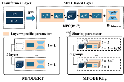
Cross-layer Parameter Sharing. To introduce our architecture, we consider a simplified structure of layers, each consisting of a single matrix. With the five-order MPO decomposition (i.e., ), we can obtain the decomposition results for a weight matrix (), denoted as , where and are the central tensor and auxiliary tensors of the -th layer. Our approach is to set a shared central tensor across layers, which means that (). As shown in Gao et al. (2020a), the central tensor contains the major proportion of parameters (more than 90%), and thus our method can largely reduce the parameters when scaling a PLM to very deep architecture. Note that this strategy can be easily applied to multiple matrices in a Transformer layer, and we omit the discussion for the multi-matrix extension. Another extension is to share the central tensor by different grouping layers. We implement a layer-grouping MPOBERT, named MPOBERT+, which divides the layers into multiple parts and sets unique shared central tensors in each group.
Layer-specific Weight Adaptation. Unlike ALBERT Lan et al. (2019), our MPO-based architecture enables layer-specific adaptation by keeping layer-specific auxiliary tensors (). These auxiliary tensors are decomposed from the original matrix, instead of extra blocks Zhang et al. (2022). They only contain a very small proportion of parameters, which does not significantly increase the model size. While, another merit of MPO decomposition is that these tensors are highly correlated via bond dimensions, and a small perturbation on an auxiliary tensor can reflect the whole matrix Liu et al. (2021). If the downstream task requires more layer specificity, we can further incorporate low-rank adapters Hu et al. (2021) for layer-specific adaptation. Specifically, we denote as the low-rank adapter for . In this way, can be formulated as a set of tensors: . The parameter scale of adapters, , is determined by the layer number , the rank , and the shape of the original matrix ( is the sum of the input and output dimensions of a Transformer Layer). Since we employ low-rank adapters, we can effectively control the number of additional parameters from adapters.
3.3 Stable Training for MPOBERT
With the above MPO-based approach, we can scale a PLM to a deeper architecture in a highly parameter-efficient way. However, as shown in prior studies Lan et al. (2019); Wang et al. (2022), it is difficult to optimize very deep PLMs, especially when shared components are involved. In this section, we introduce a simple yet stable training algorithm for MPOBERT and then discuss how it addresses the training instability issue.
3.3.1 MPO-based Network Initialization
Existing work has found that parameter initialization is important for training deep models Huang et al. (2020); Zhang et al. (2019); Wang et al. (2022), which can help alleviate the training instability. To better optimize the scaling MPOBERT, we propose a specially designed initialization method based on the above MPO-based architecture.
Initialization with MPO Decomposition. Since MPOBERT shares global components (i.e., the central tensor) across all layers, our idea is to employ existing well-trained PLMs based on weight sharing for improving parameter initialization. Here, we use the released 24-layer ALBERT with all the parameters shared across layers. The key idea is to perform MPO decomposition on the parameter matrices of ALBERT, and obtain the corresponding central and auxiliary tensors. Next, we discuss the initialization of MPOBERT in two aspects. For central tensors, we directly initialize them (each for each matrix) by the derived central tensors from the MPO decomposition results of ALBERT. Since they are globally shared, one single copy is only needed for initialization regardless of the layer depth. Similarly, for auxiliary tensors, we can directly copy the auxiliary tensors from the MPO decomposition results of ALBERT.
Scaling the Initialization. A potential issue is that ALBERT only provides a 24-layer architecture, and such a strategy no longer supports the initialization for an architecture of more than 24 layers (without corresponding auxiliary tensors). As our solution, we borrow the idea in Wang et al. (2022) that avoids the exploding update by incorporating an additional scaling coefficient and multiplying the randomly initialized values for the auxiliary tensors (those in higher than 24 layers) with a coefficient of , where is the layer number. Next, we present a theoretical analysis of training stability.
3.3.2 Theoretical Analysis
To understand the issue of training instability from a theoretical perspective, we consider a Transformer-based model with and as input and parameters, and consider one-step update 111. According to Wang et al. (2022), a large model update () at the beginning of training is likely to cause the training instability of deep Transformer models. To mitigate the exploding update problem, the update should be bounded by a constant, i.e., . Next, we study how the is bounded with the MPOBERT.
MPO-based Update Bound. Without loss of generality, we consider a simple case of low-order MPO decomposition: in Eq. (1). Following the derivation method in Wang et al. (2022), we simplify the matrices , , and to scalars ,,,, which means the parameter at the -th layer can be decomposed as . Based on these notations, we consider -layer Transformer-based model , where each sub-layer is normalized with Post-LN: . Then we can prove satisfies (see Theorem A.1 in the Appendix):
| (2) |
The above equation bounds the model update in terms of the central and auxiliary tensors. Since central tensors () can be initialized using the pre-trained weights, we can further simplify the above bound by reducing them. With some derivations (See Corollary A.2 in the Appendix), we can obtain in order to guarantee that . For simplicity, we set to bound the magnitude of each update independent of layer number . In the implementation, we first adopt the Xavier method for initialization, and then scale the parameter values with the coefficient of .
Comparison. Previous research has shown that using designed values for random initialization can improve the training of deep models (Huang et al., 2020; Zhang et al., 2019; Wang et al., 2022). These methods aim to improve the initialization of general Transformer architectures for training from scratch. As a comparison, we explore the use of pre-trained weights and employ the MPO decomposition results for initialization. In particular, Gong et al. (2019) have demonstrated the effectiveness of stacking pre-trained shallow layers for deep models in accelerating convergence, also showing performance superiority of pre-trained weights over random initialization.
3.3.3 Training and Acceleration
To instantiate our approach, we pre-train a 48-layer BERT model (i.e., MPOBERT48). For a fair comparison with BERTBASE and BERTLARGE, we adopt the same pre-training corpus (BOOKCORPUS (Zhu et al., 2015) and English Wikipedia (Devlin et al., 2018)) and pre-training tasks (masked language modeling, and sentence-order prediction). We first perform MPO decomposition on the weights of ALBERT and employ the initialization algorithm in Section 3.3.1 to set the parameter weights. During the training, we need to keep an updated copy of central tensors and auxiliary tensors: we optimize them according to the pre-training tasks in an end-to-end way and combine them to derive the original parameter matrix for forward computation (taking a relatively small cost of parallel matrix multiplication).
Typically, the speed of the pre-training process is affected by three major factors: arithmetic bandwidth, memory bandwidth, or latency. We further utilize a series of efficiency optimization ways to accelerate the pre-training, such as mixed precision training with FP16 (reducing memory and arithmetic bandwidth) and fused implementation of activation and normalization (reducing latency). Finally, we can train the 48-layer MPOBERT at a time cost of 3.8 days (compared with a non-optimized cost of 12.5 days) on our server configuration (8 NVIDIA V100 GPU cards and 32GB memory). More training details are can be found in the experimental setup Section 4.1 and Appendix A.2 (Table 6 and Algorithm 1).
4 Experiments
In this section, we first set up the experiments and then evaluate the efficiency of MPOBERT on a variety of tasks with different model settings.
4.1 Experimental Setup
Pre-training Setup. For the architecture, we denote the number of layers as , the hidden size as , and the number of self-attention heads as . We report results on four model sizes: MPOBERT (=12, =768, =12), MPOBERT (=24, =1024, =16), MPOBERT (=48, =1024, =16) and MPOBERT that implement cross-layer parameter sharing in three distinct groups as discussed in subsection 3.2.2. We pre-train all of the models with a batch size of 4096 for 10 steps. Our code will be released after the review period.
Fine-tuning Datasets. To evaluate the performance of our model, we conduct experiments on the GLUE (Wang et al., 2018) and SQuAD v1.1 (Rajpurkar et al., 2016) benchmarks. Since fine-tuning is typically fast, we run an exhaustive parameter search and choose the model that performs best on the development set to make predictions on the test set. We include the details in the Appendix(see Appendix A.3.1 for the datasets and Appendix A.3.2 for evaluation metrics)
| Experiments | MRPC | SST-2 | CoLA | RTE | STS-B | QQP | MNLI | QNLI | SQuAD | Avg. | #To (M) |
| F1 | Acc. | Mcc. | Acc. | Spear. | F1/Acc. | Acc. | Acc. | F1 | |||
| Development set | |||||||||||
| Tiny Models (#To < 50M) | |||||||||||
| ALBERT12 | 89.0 | 90.6 | 53.4 | 71.1 | 88.2 | -/89.1 | 84.5 | 89.4 | 89.3 | 82.7 | 11 |
| ALBERT24 | 84.6 | 93.6 | 52.5 | 79.8 | 90.1 | -/88.1 | 85.0 | 91.7 | 90.6 | 84.0 | 18 |
| MPOBERT12 | 90.3 | 92.3 | 55.2 | 71.8 | 90.5 | -/90.1 | 84.7 | 91.2 | 90.1 | 84.0 | 20 |
| MPOBERT24 | 90.3 | 94.4 | 58.1 | 75.5 | 91.1 | -/90.2 | 87.0 | 92.6 | 92.3 | 85.7 | 46 |
| Small Models (50M < #To < 100M) | |||||||||||
| T512 | 89.2 | 94.7 | 53.5 | 71.7 | 91.2 | -/91.1 | 87.8 | 93.8 | 90.0 | 84.8 | 60 |
| MPOBERT48 | 90.8 | 94.7 | 58.3 | 77.3 | 91.4 | -/89.5 | 86.3 | 92.0 | 92.3 | 85.8 | 75 |
| Base Models (#To > 100M) | |||||||||||
| BERT12 | 90.7 | 91.7 | 48.9 | 71.4 | 91.0 | -/90.8 | 83.7 | 89.3 | 88.5 | 82.9 | 110 |
| XLNet12 | 85.3 | 94.4 | 49.3 | 63.9 | 85.6 | -/90.7 | 90.9 | 91.8 | 90.2 | 82.5 | 117 |
| RoBERTa12 | 91.9 | 92.2 | 59.4 | 72.2 | 89.4 | -/91.2 | 88.0 | 92.7 | 91.2 | 85.4 | 125 |
| BART12 | 91.4 | 93.8 | 56.3 | 79.1 | 89.9 | -/90.8 | 86.4 | 92.4 | 91.6 | 82.8 | 140 |
| MPOBERT48+ | 89.7 | 94.4 | 57.4 | 79.8 | 91.1 | -/89.3 | 87.1 | 92.4 | 91.4 | 86.0 | 102 |
| Test set | |||||||||||
| Tiny Models (#To < 50M) | |||||||||||
| ALBERT12 | 89.2 | 93.2 | 53.6 | 70.2 | 87.3 | 70.3/- | 84.6 | 92.5 | 89.3 | 81.1 | 11 |
| ALBERT24 | 88.7 | 94.0 | 51.7 | 73.7 | 86.9 | 69.1/- | 84.9 | 91.8 | 90.6 | 81.2 | 18 |
| MobileBERT24 | 88.8 | 92.6 | 51.1 | 70.4 | 84.8 | 70.5/- | 83.3 | 91.6 | 90.3 | 80.4 | 25 |
| MPOBERT12 | 89.2 | 91.9 | 52.7 | 70.6 | 87.1 | 69.6/- | 85.0 | 91.0 | 90.1 | 80.8 | 20 |
| MPOBERT24 | 89.0 | 94.5 | 55.5 | 73.4 | 88.2 | 71.0/- | 86.3 | 93.0 | 92.3 | 82.6 | 46 |
| Small Models (50M < #To < 100M) | |||||||||||
| T512 | 89.7 | 91.8 | 41.0 | 69.9 | 85.6 | 70.0/- | 82.4 | 90.3 | 90.0 | 78.7 | 60 |
| TinyBERT6 | 87.3 | 93.1 | 51.1 | 70.0 | 83.7 | 71.6/- | 84.6 | 90.4 | 87.5 | 79.9 | 67 |
| DistilBERT6 | 86.9 | 92.5 | 49.0 | 58.4 | 81.3 | 70.1/- | 82.6 | 88.9 | 86.2 | 77.3 | 67 |
| MPOBERT48 | 90.0 | 94.0 | 55.0 | 74.0 | 88.7 | 71.0/- | 86.5 | 91.8 | 92.3 | 82.6 | 75 |
| Base Models (#To > 100M) | |||||||||||
| BERT12 | 88.9 | 93.5 | 52.1 | 66.4 | 85.8 | 71.2/- | 84.6 | 90.5 | 88.5 | 79.1 | 110 |
| XLNet12 | 89.2 | 94.3 | 47.3 | 66.5 | 85.4 | 71.9/- | 87.1 | 91.4 | 90.2 | 80.4 | 117 |
| RoBERTa12 | 89.9 | 93.2 | 57.9 | 69.9 | 88.3 | 72.5/- | 87.7 | 92.5 | 91.2 | 82.6 | 125 |
| BART12 | 89.9 | 93.7 | 49.6 | 72.6 | 86.9 | 71.7/- | 84.9 | 92.3 | 91.6 | 81.5 | 140 |
| MPOBERT48+ | 89.9 | 94.5 | 56.0 | 74.5 | 88.4 | 70.5/- | 86.5 | 92.6 | 91.4 | 82.7 | 102 |
Baseline Models. We compare our proposed MPOBERT to the existing competitive deep PLMs and parameter-efficient models. In order to make fair comparisons, we divide the models into three major categories based on their model sizes:
Tiny Models (#To < 50M). ALBERT12 Lan et al. (2019) is the most representative PLM that achieves competitive results with only 11M.
Small models (50M< #To <100M). We consider PLMs (T512) and compressed models (MobileBERT (Sun et al., 2020b), DistilBERT (Sanh et al., 2019) and TinyBERT (Jiao et al., 2019)).
Base models (#To > 100M). We compare with BERT12, XLNet12, RoBERTa12 and BART12 for this category. Note that we only include the base variants that have similar model sizes in order to make a fair comparison.
More details about the baseline models are described in Appendix A.3.3.
4.2 Main Results
Fully-supervised setting. We present the results of MPOBERT and other baseline models on GLUE and Squad for fine-tuning in Table 1.
Firstly, we evaluate MPOBERT’s performance in comparison to other models with similar numbers of parameters. In particular, for tiny models, MPOBERT24 outperforms ALBERT24, and achieves substantial improvements on both the development set (85.7 v.s. 84.0) and test sets (82.6 v.s. 81.2). This highlights the benefits of increased capacity from layer-specific parameters (i.e., the auxiliary tensors and layer-specific adapters) in MPOBERT. Furthermore, for small and base models, 48-layer MPOBERT consistently achieves better results than T512 and all parameter-efficient models, while also achieving comparable results to other 12-layer PLMs with a reduced number of parameters. This demonstrates the significant benefits of scaling along the model depth with layer-specific parameters in MPOBERT.
Secondly, we assess MPOBERT’s parameter efficiency by comparing it to other PLMs within the same model depth. For instance, when considering models with =12 layers, MPOBERT achieves comparable results or even outperforms (+1.7 for BERT12 and +0.4 for XLNet12) PLMs while having fewer parameters. This further highlights the advantages of MPOBERT’s parameter-efficient approach in constructing deep models.
Multitask Fine-tuning Setting. To demonstrate the effectiveness of our proposed parameter-sharing model in learning shared representations across multiple tasks, we fine-tune MPOBERT, BERT and ALBERT on the multitask GLUE benchmark and report the results in Table 2. Specifically, we design two groups of experiments. (1) Deep vs. shallow models. Comparing with BERT12, MPOBERT48 has much deeper Transformer layers but still fewer total parameters (i.e., 75M vs. 110M). We find that MPOBERT48 achieves 1.4 points higher on average GLUE score than BERT12. (2) Central tensors sharing vs. all weight sharing. Comparing with ALBERT12, MPOBERT12 only shares part of weights, i.e., central tensors, while ALBERT12 shares all of the weights. We find that sharing central tensors may effectively improve the average results than sharing all weights (82.0 v.s. 81.4 for MRPC).
| Datasets | B12 | M48 | M12 | A12 |
| MNLI (Acc.) | 83.9 | 85.4 | 82.8 | 82.7 |
| QNLI (Acc.) | 90.8 | 91.1 | 90.0 | 89.4 |
| SST-2 (Acc.) | 91.7 | 93.0 | 90.9 | 90.6 |
| RTE (Acc.) | 81.2 | 82.0 | 79.8 | 79.1 |
| QQP (Acc.) | 91.2 | 87.6 | 90.4 | 89.7 |
| CoLA (Mcc.) | 53.6 | 54.9 | 45.0 | 35.9 |
| MRPC (F1) | 84.2 | 91.8 | 89.9 | 89.2 |
| STS-B (Spear.) | 87.4 | 89.0 | 86.9 | 87.5 |
| Avg. | 83.0 | 84.4 | 82.0 | 80.5 |
| #To (M) | 110 | 75 | 20 | 11 |
Few-shot Learning Setting.
| SST-2 | MNLI | |||||
| Shots (K) | 10 | 20 | 30 | 10 | 20 | 30 |
| BERT12 | 54.8 | 59.7 | 61.6 | 37.0 | 35.6 | 35.7 |
| ALBERT12 | 56.7 | 59.3 | 60.0 | 36.3 | 35.6 | 36.5 |
| MPOBERT12 | 58.9 | 65.4 | 64.6 | 36.7 | 36.7 | 37.1 |
We evaluate the performance of our proposed model, MPOBERT, in few-shot learning setting Huang et al. (2022) on two tasks, SST-2 and MNLI, using a limited number of labeled examples. Results in Table 3 show that MPOBERT outperforms BERT, which suffers from over-fitting, and ALBERT, which does not benefit from its reduced number of parameters. These results further demonstrate the superiority of our proposed model in exploiting the potential of large model capacity under limited data scenarios.
4.3 Detailed Analysis
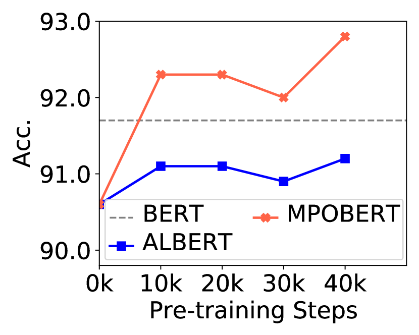
Analysis of Initialization Methods. This experiment aims to exclude the effect of initialized pre-trained weights on fine-tuning results. We plot the performance of the model on SST-2 w.r.t training steps. In particular, we compare the performance of MPOBERT using different initialization methods (Xavier in Fig. 3(a) and decomposed weights of ALBERT in Fig. 3(b)) for pre-training. The results demonstrate that pre-training MPOBERT from scratch requires around 50 steps to achieve performance comparable to BERTBASE, while initializing with the decomposed weights of ALBERT significantly accelerates convergence and leads to obvious improvements within the first 10 training steps. In contrast, the gains from continual pre-training for ALBERT are negligible. These results provide assurance that the improvements observed in MPOBERT are not solely attributed to the use of initialized pre-trained weights.
| Experiment | SST-2 | RTE | MRPC | #To (M) |
| MPOBERT12 | 92.8 | 72.9 | 91.8 | 20.0 |
| w/o Adapter | 92.3 | 71.8 | 90.3 | 19.4 |
| w/o PS | 91.4 | 67.9 | 85.8 | 11.9 |
Ablation Analysis. To assess the individual impact of the components in our MPOBERT model, we conduct an ablation study by removing either the layer-specific adapter or the cross-layer parameter-sharing strategy. The results, displayed in Table 4, indicate that the removal of either component results in a decrease in the model’s performance, highlighting the importance of both components in our proposed strategy. While the results also indicate that cross-layer parameter sharing plays a more crucial role in the model’s performance.
| Rank | SST-2 | RTE | MRPC | #To (M) |
| 4 | 91.9 | 69.7 | 88.2 | 19.7 |
| 8 | 92.8 | 72.9 | 91.8 | 20.0 |
| 64 | 91.6 | 69.3 | 88.1 | 24.3 |
Performance Comparison w.r.t Adapter Rank. To compare the impact of the adapter rank in layer-specific adapters on MPOBERT’s performance, we trained MPOBERT with different ranks (4,8 and 64) and evaluate the model on downstream tasks in Table 5. The results demonstrate that a rank of 8 is sufficient for MPOBERT, which further shows the necessity of layer-specific adapters. However, we also observe a decrease in the performance of the variant with adapter rank 64. This illustrates that further increasing the rank may increase the risk of over-fitting in fine-tuning process. Therefore, we set a rank of 8 for MPOBERT in the main results.
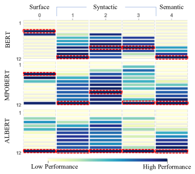
Analysis of Linguistic Patterns. To investigate the linguistic patterns captured by MPOBERT, BERT, and ALBERT, we conduct a suite of probing tasks, following the methodology of Tenney et al. (2019). These tasks are designed to evaluate the encoding of surface, syntactic, and semantic information in the models’ representations. The results, shown in Fig. 4, reveal that BERT encodes more local syntax in lower layers and more complex semantics in higher layers, while ALBERT does not exhibit such a clear trend. However, MPOBERT exhibits similar layer-wise behavior to BERT in some tasks (i.e., task 0,2,4), and improved results in lower layers for others (i.e., task 3) which is similar to ALBERT. The result demonstrates that MPOBERT captures linguistic information differently than other models, and its layer-wise parameters play an important role in this difference.
5 Conclusion
We develop MPOBERT, a parameter-efficient pre-trained language model that allows for the efficient scaling of deep models without the need for additional parameters or computational resources. We achieve this by introducing an MPO-based Transformer layer and sharing the central tensors across layers. During training, we propose initialization methods for the central and auxiliary tensors, which are based on theoretical analysis to address training stability issues. The effectiveness of MPOBERT is demonstrated through various experiments, such as supervised, multitasking, and few-shot where it consistently outperforms other competing models.
Limitations
The results presented in our study are limited by some natural language processing tasks and datasets that are evaluated, and further research is needed to fully understand the interpretability and robustness of our MPOBERT models. Additionally, there is subjectivity in the selection of downstream tasks and datasets, despite our use of widely recognized categorizations from the literature. Furthermore, the computational constraints limited our ability to study the scaling performance of the MPOBERT model at deeper depths such as 96 layers or more. This is an area for future research.
Ethics Statement
The use of a large corpus for training large language models may raise ethical concerns, particularly regarding the potential for bias in the data. In our study, we take precautions to minimize this issue by utilizing only standard training data sources, such as BOOKCORPUS and Wikipedia, which are widely used in language model training Devlin et al. (2018); Lan et al. (2019). However, it is important to note that when applying our method to other datasets, the potential bias must be carefully considered and addressed. Further investigation and attention should be given to this issue in future studies.
References
- Chen et al. (2020) Tianlong Chen, Jonathan Frankle, Shiyu Chang, Sijia Liu, Yang Zhang, Zhangyang Wang, and Michael Carbin. 2020. The lottery ticket hypothesis for pre-trained BERT networks. In Advances in Neural Information Processing Systems 33: Annual Conference on Neural Information Processing Systems 2020, NeurIPS 2020, December 6-12, 2020, virtual.
- Chowdhery et al. (2022) Aakanksha Chowdhery, Sharan Narang, Jacob Devlin, Maarten Bosma, Gaurav Mishra, Adam Roberts, Paul Barham, Hyung Won Chung, Charles Sutton, Sebastian Gehrmann, Parker Schuh, Kensen Shi, Sasha Tsvyashchenko, Joshua Maynez, Abhishek Rao, Parker Barnes, Yi Tay, Noam Shazeer, Vinodkumar Prabhakaran, Emily Reif, Nan Du, Ben Hutchinson, Reiner Pope, James Bradbury, Jacob Austin, Michael Isard, Guy Gur-Ari, Pengcheng Yin, Toju Duke, Anselm Levskaya, Sanjay Ghemawat, Sunipa Dev, Henryk Michalewski, Xavier Garcia, Vedant Misra, Kevin Robinson, Liam Fedus, Denny Zhou, Daphne Ippolito, David Luan, Hyeontaek Lim, Barret Zoph, Alexander Spiridonov, Ryan Sepassi, David Dohan, Shivani Agrawal, Mark Omernick, Andrew M. Dai, Thanumalayan Sankaranarayana Pillai, Marie Pellat, Aitor Lewkowycz, Erica Moreira, Rewon Child, Oleksandr Polozov, Katherine Lee, Zongwei Zhou, Xuezhi Wang, Brennan Saeta, Mark Diaz, Orhan Firat, Michele Catasta, Jason Wei, Kathy Meier-Hellstern, Douglas Eck, Jeff Dean, Slav Petrov, and Noah Fiedel. 2022. Palm: Scaling language modeling with pathways. CoRR, abs/2204.02311.
- Devlin et al. (2018) Jacob Devlin, Ming-Wei Chang, Kenton Lee, and Kristina Toutanova. 2018. Bert: Pre-training of deep bidirectional transformers for language understanding. arXiv preprint arXiv:1810.04805.
- Gao et al. (2020a) Ze-Feng Gao, Song Cheng, Rong-Qiang He, Zhi-Yuan Xie, Hui-Hai Zhao, Zhong-Yi Lu, and Tao Xiang. 2020a. Compressing deep neural networks by matrix product operators. Physical Review Research, 2(2):023300.
- Gao et al. (2022) Ze-Feng Gao, Peiyu Liu, Wayne Xin Zhao, Zhong-Yi Lu, and Ji-Rong Wen. 2022. Parameter-efficient mixture-of-experts architecture for pre-trained language models. In Proceedings of the 29th International Conference on Computational Linguistics, COLING 2022, Gyeongju, Republic of Korea, October 12-17, 2022, pages 3263–3273. International Committee on Computational Linguistics.
- Gao et al. (2020b) Ze-Feng Gao, Xingwei Sun, Lan Gao, Junfeng Li, and Zhong-Yi Lu. 2020b. Compressing lstm networks by matrix product operators. arXiv preprint arXiv:2012.11943.
- Garipov et al. (2016) Timur Garipov, Dmitry Podoprikhin, Alexander Novikov, and Dmitry Vetrov. 2016. Ultimate tensorization: compressing convolutional and fc layers alike. arXiv preprint arXiv:1611.03214.
- Gong et al. (2019) Linyuan Gong, Di He, Zhuohan Li, Tao Qin, Liwei Wang, and Tie-Yan Liu. 2019. Efficient training of BERT by progressively stacking. In Proceedings of the 36th International Conference on Machine Learning, ICML 2019, 9-15 June 2019, Long Beach, California, USA, volume 97 of Proceedings of Machine Learning Research, pages 2337–2346. PMLR.
- Hu et al. (2021) Edward J Hu, Yelong Shen, Phillip Wallis, Zeyuan Allen-Zhu, Yuanzhi Li, Shean Wang, Lu Wang, and Weizhu Chen. 2021. Lora: Low-rank adaptation of large language models. arXiv preprint arXiv:2106.09685.
- Huang et al. (2020) Xiao Shi Huang, Felipe Pérez, Jimmy Ba, and Maksims Volkovs. 2020. Improving transformer optimization through better initialization. In Proceedings of the 37th International Conference on Machine Learning, ICML 2020, 13-18 July 2020, Virtual Event, volume 119 of Proceedings of Machine Learning Research, pages 4475–4483. PMLR.
- Huang et al. (2022) Zixian Huang, Ao Wu, Jiaying Zhou, Yu Gu, Yue Zhao, and Gong Cheng. 2022. Clues before answers: Generation-enhanced multiple-choice QA. In Proceedings of the 2022 Conference of the North American Chapter of the Association for Computational Linguistics: Human Language Technologies, pages 3272–3287, Seattle, United States. Association for Computational Linguistics.
- Jiao et al. (2019) Xiaoqi Jiao, Yichun Yin, Lifeng Shang, Xin Jiang, Xiao Chen, Linlin Li, Fang Wang, and Qun Liu. 2019. Tinybert: Distilling bert for natural language understanding. arXiv preprint arXiv:1909.10351.
- Kaplan et al. (2020) Jared Kaplan, Sam McCandlish, Tom Henighan, Tom B. Brown, Benjamin Chess, Rewon Child, Scott Gray, Alec Radford, Jeffrey Wu, and Dario Amodei. 2020. Scaling laws for neural language models. CoRR, abs/2001.08361.
- Lan et al. (2019) Zhenzhong Lan, Mingda Chen, Sebastian Goodman, Kevin Gimpel, Piyush Sharma, and Radu Soricut. 2019. Albert: A lite bert for self-supervised learning of language representations. arXiv preprint arXiv:1909.11942.
- Liu et al. (2021) Peiyu Liu, Ze-Feng Gao, Wayne Xin Zhao, Zhi-Yuan Xie, Zhong-Yi Lu, and Ji-Rong Wen. 2021. Enabling lightweight fine-tuning for pre-trained language model compression based on matrix product operators. In Proceedings of the 59th Annual Meeting of the Association for Computational Linguistics and the 11th International Joint Conference on Natural Language Processing (Volume 1: Long Papers), pages 5388–5398.
- Liu et al. (2020) Weijie Liu, Peng Zhou, Zhe Zhao, Zhiruo Wang, Haotang Deng, and Qi Ju. 2020. Fastbert: a self-distilling bert with adaptive inference time. arXiv preprint arXiv:2004.02178.
- Michel et al. (2019) Paul Michel, Omer Levy, and Graham Neubig. 2019. Are sixteen heads really better than one? In Advances in Neural Information Processing Systems 32: Annual Conference on Neural Information Processing Systems 2019, NeurIPS 2019, December 8-14, 2019, Vancouver, BC, Canada, pages 14014–14024.
- Nouriborji et al. (2022) Mohammadmahdi Nouriborji, Omid Rohanian, Samaneh Kouchaki, and David A. Clifton. 2022. Minialbert: Model distillation via parameter-efficient recursive transformers. CoRR, abs/2210.06425.
- Novikov et al. (2015) Alexander Novikov, Dmitry Podoprikhin, Anton Osokin, and Dmitry Vetrov. 2015. Tensorizing neural networks. arXiv preprint arXiv:1509.06569.
- Oseledets (2011) Ivan V Oseledets. 2011. Tensor-train decomposition. SIAM Journal on Scientific Computing, 33(5):2295–2317.
- Radford et al. (2019) Alec Radford, Jeffrey Wu, Rewon Child, David Luan, Dario Amodei, Ilya Sutskever, et al. 2019. Language models are unsupervised multitask learners. OpenAI blog, 1(8):9.
- Raffel et al. (2020) Colin Raffel, Noam Shazeer, Adam Roberts, Katherine Lee, Sharan Narang, Michael Matena, Yanqi Zhou, Wei Li, Peter J Liu, et al. 2020. Exploring the limits of transfer learning with a unified text-to-text transformer. J. Mach. Learn. Res., 21(140):1–67.
- Rajpurkar et al. (2016) Pranav Rajpurkar, Jian Zhang, Konstantin Lopyrev, and Percy Liang. 2016. SQuAD: 100,000+ questions for machine comprehension of text. In Proceedings of the 2016 Conference on Empirical Methods in Natural Language Processing, pages 2383–2392, Austin, Texas. Association for Computational Linguistics.
- Reid et al. (2021) Machel Reid, Edison Marrese-Taylor, and Yutaka Matsuo. 2021. Subformer: Exploring weight sharing for parameter efficiency in generative transformers. In Findings of the Association for Computational Linguistics: EMNLP 2021, pages 4081–4090, Punta Cana, Dominican Republic. Association for Computational Linguistics.
- Sanh et al. (2019) Victor Sanh, Lysandre Debut, Julien Chaumond, and Thomas Wolf. 2019. Distilbert, a distilled version of bert: smaller, faster, cheaper and lighter. arXiv preprint arXiv:1910.01108.
- Sun et al. (2020a) Xingwei Sun, Ze-Feng Gao, Zhong-Yi Lu, Junfeng Li, and Yonghong Yan. 2020a. A model compression method with matrix product operators for speech enhancement. IEEE/ACM Transactions on Audio, Speech, and Language Processing, 28:2837–2847.
- Sun et al. (2020b) Zhiqing Sun, Hongkun Yu, Xiaodan Song, Renjie Liu, Yiming Yang, and Denny Zhou. 2020b. Mobilebert: a compact task-agnostic bert for resource-limited devices. arXiv preprint arXiv:2004.02984.
- Tenney et al. (2019) Ian Tenney, Patrick Xia, Berlin Chen, Alex Wang, Adam Poliak, R. Thomas McCoy, Najoung Kim, Benjamin Van Durme, Samuel R. Bowman, Dipanjan Das, and Ellie Pavlick. 2019. What do you learn from context? probing for sentence structure in contextualized word representations. In 7th International Conference on Learning Representations, ICLR 2019, New Orleans, LA, USA, May 6-9, 2019. OpenReview.net.
- Wang et al. (2018) Alex Wang, Amanpreet Singh, Julian Michael, Felix Hill, Omer Levy, and Samuel R Bowman. 2018. Glue: A multi-task benchmark and analysis platform for natural language understanding. arXiv preprint arXiv:1804.07461.
- Wang et al. (2022) Hongyu Wang, Shuming Ma, Li Dong, Shaohan Huang, Dongdong Zhang, and Furu Wei. 2022. Deepnet: Scaling transformers to 1, 000 layers. CoRR, abs/2203.00555.
- Wang et al. (2020) Ziheng Wang, Jeremy Wohlwend, and Tao Lei. 2020. Structured pruning of large language models. In Proceedings of the 2020 Conference on Empirical Methods in Natural Language Processing, EMNLP 2020, Online, November 16-20, 2020, pages 6151–6162. Association for Computational Linguistics.
- You et al. (2020) Yang You, Jing Li, Sashank J. Reddi, Jonathan Hseu, Sanjiv Kumar, Srinadh Bhojanapalli, Xiaodan Song, James Demmel, Kurt Keutzer, and Cho-Jui Hsieh. 2020. Large batch optimization for deep learning: Training BERT in 76 minutes. In 8th International Conference on Learning Representations, ICLR 2020, Addis Ababa, Ethiopia, April 26-30, 2020. OpenReview.net.
- Yu et al. (2017) Rose Yu, Stephan Zheng, Anima Anandkumar, and Yisong Yue. 2017. Long-term forecasting using tensor-train rnns. Arxiv.
- Zhang et al. (2019) Hongyi Zhang, Yann N. Dauphin, and Tengyu Ma. 2019. Fixup initialization: Residual learning without normalization. In 7th International Conference on Learning Representations, ICLR 2019, New Orleans, LA, USA, May 6-9, 2019. OpenReview.net.
- Zhang et al. (2022) Jinnian Zhang, Houwen Peng, Kan Wu, Mengchen Liu, Bin Xiao, Jianlong Fu, and Lu Yuan. 2022. Minivit: Compressing vision transformers with weight multiplexing. In IEEE/CVF Conference on Computer Vision and Pattern Recognition, CVPR 2022, New Orleans, LA, USA, June 18-24, 2022, pages 12135–12144. IEEE.
- Zhu et al. (2015) Yukun Zhu, Ryan Kiros, Rich Zemel, Ruslan Salakhutdinov, Raquel Urtasun, Antonio Torralba, and Sanja Fidler. 2015. Aligning books and movies: Towards story-like visual explanations by watching movies and reading books. In Proceedings of the IEEE international conference on computer vision, pages 19–27.
Appendix A Appendix
A.1 Proofs
Notations.
We denote as the loss function. as the standard layer normalization with scale and bias . Let denote standard Big-O notation that suppresses multiplicative constants. stands for equal bound of magnitude. We aim to study the magnitude of the model updates. We define the model update as .
Definition is updated by per SGD step after initialization as . That is, where can be calculated through .
Theorem A.1
Given an -layer transformer-based model , where denotes the parameters in -th layer and each sub-layer is normalized with Post-LN: . In MPOBERT, is decomposed by MPO to local tensors: , and we share across layers: . Then satisfies:
| (3) |
We follow Zhang et al. (2019) and make the following assumptions to simplify the derivations:
-
1.
Hidden dimension equals to ;
-
2.
;
-
3.
All relevant weights are positive with magnitude less than .
Given Assumption 1, if is MLP with the weight , then . With assumption 2, we have:
| (4) | ||||
| (5) |
Then, with Taylor expansion, the model update satisfies:
| (6) |
With Eq. (5), the magnitude of and is bounded by:
| (7) | |||
| (8) |
Since we apply MPO decomposition to , we get:
| (9) |
For simplicity, we reduce the matrices ,, to the scalars ,,. Thus with Assumption 3, Eq. (6) is reformulated as: Finally, with Assumption 3 we have:
| (10) | ||||
| (11) |
Corollary A.2
Given that we initialise in MPOBERT with well-trained weights, it is reasonable to assume that updates of are well-bounded. Then satisfies when for all :
| (12) |
For an -layer MPOBERT, we have:
| (13) | ||||
| (14) |
By assumption and , we achieve:
| (15) | ||||
| (16) |
Finally, we achieve:
| (17) |
Due to symmetry, we set , . Thus, from A.1, we set to achieve to bound the magnitudes of each update to be independent of model depth , i.e., .
A.2 Training Details
A.2.1 Details of Training
Here we describe the details of the pre-training process in Algorithm 1. For pre-training, we tune the learning rate in the range of [, ] and use the LAMB optimizer You et al. (2020). Since fine-tuning is typically fast, we run an exhaustive parameter search (i.e., learning rate in the range of [, ], batch size in {8,16,32}) and choose the model that performs best on the development set to make predictions on the test set.
A.2.2 Details of Training Configurations
In this part, we list the training configurations of MPOBERT and other representative PLMs in Table 6.
| Models | #To (M) | Depth | Samples | Training time | GLUR Dev. | GLUE Test |
| T511B | 11000 | 24 | - | - | - | 89.0 |
| T5BASE | 220 | 24 | 128 524 | 16 TPU v3 1 Day (t5-base) | 84.1 | 82.5 |
|---|---|---|---|---|---|---|
| BERTLARGE | 330 | 24 | 256 1000 | 16 Cloud TPUs 4 Days | 84.1 | 81.6 |
| ALBERTXXLARGE | 235 | 1 | 4096 1.5 | TPU v3 16 Days | 90.0 | - |
| BARTLARGE | 407 | 24 | 8000 500 | - | 88.8 | - |
| RoBERTaLARGE | 355 | 24 | 8000 500 | 1024 V100 GPUs 1 Day | 88.9 | - |
| XLNetLARGE | 361 | 24 | 8192 500 | 512 TPU v3 5.5 Days | 87.4 | - |
| MPOBERT48+ | 102 | 48 | 4096 10 | 8 V100 GPUs 3.8 Days | 85.6 | 81.7 |
A.3 Experimental Details
A.3.1 Details of Fine-tuning Datasets
GLUE benchmark covers multiple datasets (MNLI, QNLI, QQP, CoLA, RTE, MRPC, SST-2) 222In line with Raffel et al. (2020), we do not test WNLI due to its adversarial character with respect to the training set.. The SQuAD is a collection of 100 crowd-sourced question/answer pairs. Given a question and a passage, the task is to predict the answer text span in the passage.
A.3.2 Details of Evaluation Metrics
Following Gao et al. (2022), we employ Matthew’s correlation for CoLA, Spearman for STS-B, F1 for MRPC, and accuracy for the remaining tasks as the metrics for the GLUE benchmark. We compute and present the average scores across all test samples for each of the aforementioned metrics.
A.3.3 Details of Baseline Models
We compare our proposed MPOBERT to the existing competitive deep PLMs and parameter-efficient models. In order to make fair comparisons, we divide the models into three major categories based on their model sizes: Tiny Models (#To < 50M). ALBERT12 Lan et al. (2019) is the most representative PLM that achieves competitive results with only 11M.
Small models (50M< #To <100M). T512 is a small variant of T5 Raffel et al. (2020) which has only 6 encoder layers and 6 decoder layers. In addition, there are three parameter-efficient Transformer models that have similar parameters, namely MobileBERT (Sun et al., 2020b), DistilBERT (Sanh et al., 2019) and TinyBERT (Jiao et al., 2019). We compare with these compressed models to show the benefit of scaling to deeper models over compressing large models to small variants.
Base models (#To > 100M). We compare with BERT12, XLNet12, RoBERTa12 and BART12 for this category. Note that we only include the base variants that have similar model sizes in order to make a fair comparison. More details about the comparison with the strongest variants are described in Appendix A.3.3.