Convolutional neural network search for long-duration transient gravitational waves from glitching pulsars

Abstract

Machine learning can be a powerful tool to discover new signal types in astronomical data. We here apply it to search for long-duration transient gravitational waves triggered by pulsar glitches, which could yield physical insight into the mostly unknown depths of the pulsar. Current methods to search for such signals rely on matched filtering and a brute-force grid search over possible signal durations, which is sensitive but can become very computationally expensive. We develop a method to search for post-glitch signals on combining matched filtering with convolutional neural networks, which reaches similar sensitivities to the standard method at false-alarm probabilities relevant for practical searches, while being significantly faster. We specialize to the Vela glitch during the LIGO–Virgo O2 run, and set upper limits on the gravitational-wave strain amplitude from the data of the two LIGO detectors for both constant-amplitude and exponentially decaying signals.

I Introduction

Gravitational wave (GW) detectors are sensitive to a variety of different sources. Spinning neutron stars (NSs) with non-axisymmetric deformations, in particular, are promising GW sources [1], e.g. for long-lasting quasi-monochromatic signals (continuous waves, CWs) [2, 3]. The expected amplitudes of CWs are several orders of magnitude smaller than the signals already detected from compact binary coalescences (CBCs) [4], requiring long integration times, and have not been discovered yet by current LIGO–Virgo–KAGRA detectors [5, 6, 7].

Pulsars are rotating NSs that also emit electromagnetic (EM) beams. Of these, some show glitches [8], i.e. rare anomalies in their otherwise very stable frequency evolution. Glitches typically feature a sudden spin-up, often followed by a relaxation phase, and are one of the few circumstances in which we may examine the inside of a NS and the characteristics of matter at supernuclear density [9]. They could also excite non-axisymmetric perturbations, hence triggering GWs [10]. These signals could be “burst-like”, with dampening timescales of milliseconds [11], and also long-duration transient CW-like signals (tCWs) with timescales from hours to months [12]. The detection of GWs from a pulsar glitch could yield more understanding of the NS equation of state [13].

Detection prospects for tCWs were studied in Ref. [14], finding that upcoming LVK observing runs will offer the first chances to detect them or at least to obtain upper limits that can physically constrain glitch models. Third generation GW detectors such as Einstein Telescope [15] and Cosmic Explorer [16] will be able to probe deeper into the population of known glitchers. The Vela pulsar (J0835$-$4510) is a particularly strong candidate, because of its large and frequent glitches, also characterized by long recovery times up to several hundred days.

Recent works have performed unmodelled searches for burst-like transients [17, 18] and modelled searches for long-duration tCWs [19, 20, 21]. In this work we focus on tCW searches, which are so far based on matched filtering of the data against a signal model. Typically, a template bank is constructed to cover the possible range of signal parameters. However these model-dependent searches are usually limited in the volume of parameter space that can be covered, due to high computational cost, as we detail in Sec. II.

A possible way out of computational bottlenecks in GW data analysis is deep learning (DL), a subfield of machine learning which consists of processing data with deep neural networks. DL has been gaining ground in different scientific fields and in particular in gravitational astronomy, as it offers powerful novel methods to search for or classify signals while decreasing computational cost. Ref. [22] offers a review of GW applications, spanning from data quality studies and detector characterization, to waveform modeling and searches using different DL model architectures. In this work we provide a DL algorithm based on a Convolutional Neural Network (CNN) as a complementary tool to matched filtering in the search for tCWs from glitching pulsars.

The paper is structured as follows. In Sec. II we set up the detection problem with a specific real-world test case (searching for tCWs after the 2016 Vela pulsar glitch), starting from matched filtering, and we motivate how DL can help with its limitations. In Sec. III we introduce our CNN architecture and training strategy and in Sec. IV we explain our evaluation method and testing sets. In Sec. V we test the CNN on simulated and real data, and in Sec. VI we consider extensions to parameter estimation. We then present observational upper limits on the strain amplitude of tCWs after the 2016 Vela glitch in Sec. VII, comparing with those previously obtained in Ref. [19]. Finally we state conclusions in Sec. VIII.

II Problem statement and a real-world test case

The standard method to search for tCWs is based on matched filtering and was first introduced in Ref. [12]. So far it has been applied in Ref. [19, 20] to search for signals from various known glitching pulsars in data from the second and third LIGO–Virgo observing runs (O2 and O3). We briefly summarize the method here and provide more details in Appendix A. Considerations for the practical setup of such searches based on the ephemerides of known pulsars are provided in Ref. [21]. The setup of this detection method is very similar to that of narrowband CW searches [20, 23, 24], but for tCWs one must also take into account additional parameters describing the temporal evolution of the signal, e.g. its start time and duration.

The pulsar population presents a large variety of glitching behaviors [8], and there are several models explaining this phenomenology [10, 9]. Similarly, GW signals could derive from different physical mechanisms, e.g. Ekman flows [25, 26, 27] or Rossby r-modes [28, 29], varying from glitch to glitch. Depending on the model, it may be reasonable to expect tCWs with durations of the order of the timescales of the post-glitch recovery, i.e. the time needed for the frequency to return to its secular value [30]. In general, searches for tCWs must account for this model uncertainty by covering wider ranges of possible parameters, including all possible combinations of the transient parameters and sufficiently wide frequency evolution template banks, of sizes up to tens of millions per target.

II.1 Current method for detecting tCWs

In matched filtering the first step is to define the signal model. We ignore the specific physical process behind the generation of the signal, and define a generic tCW model following Ref. [12], by generalizing the standard CW model.

First we introduce

$$h_{\textrm{CW}}(t;\lambda,\mathcal{A})=\sum_{\mu=0}^{3}\mathcal{A}^{\mu}h_{\mu}(t;\lambda),$$ (1)

where $h_{\mu}$ are four basis functions derived in Ref. [31], and $\lambda,\mathcal{A}$ are the frequency evolution and amplitude parameters of the signal, respectively. The four amplitude parameters depend on the CW amplitude $h_{0}$, inclination $\cos\iota$, polarization angle $\psi$, and initial phase $\phi_{0}$, while the frequency evolution parameters include the source position (right ascension $\alpha$ and declination $\delta$) and the GW frequency $f$ and spindowns (frequency derivatives) ${\dot{f}},\ddot{f},\dddot{f},\dots$ For GW emission driven by a mass quadrupole, the GW frequency and spindown values are twice the rotational values.

From Eq. (1), tCWs can be obtained by multiplying with a window function $\varpi(t;\mathcal{T})$ dependent on time and an additional set of transient parameters $\mathcal{T}$:

$$h(t;\lambda,\mathcal{A},\mathcal{T})=\varpi(t;\mathcal{T})h_{\textrm{CW}}(t;\lambda,\mathcal{A}).$$ (2)

For instance, $\mathcal{T}$ can be the start time $t^{0}$ and the duration $\tau$ of the tCW signal. Two simple choices of window functions are the rectangular window, for signals of constant amplitude truncated in time,

$$\varpi_{\textrm{r}}(t;t^{0},\tau)=\begin{cases}1&\text{if $t\in[t^{0},t^{0}+\tau]$}\\ 0&\text{otherwise}\end{cases},$$ (3)

and the exponentially decaying window

$$\varpi_{\textrm{e}}(t;t^{0},\tau)=\begin{cases}e^{-(t-t^{0})/\tau}&\text{if $t\in[t^{0},t^{0}+3\tau]$}\\ 0&\text{otherwise}\end{cases},$$ (4)

where for $\varpi_{\textrm{e}}$ the truncation at $3\tau$ was chosen by Ref. [12] as the point where the amplitude has decreased by more than 95%.

While the rectangular window follows the exact evolution of a standard CW and solely cuts it in time, the exponentially decaying window modifies the time evolution of the amplitude $h_{0}$. In general, one can define an arbitrary window function depending on different transient parameters $\mathcal{T}$, but for simplicity we only consider and compare the two choices above.

Once the signal model is defined, one can then proceed as in Ref. [12] with a noise-versus-signal hypothesis test, assuming Gaussian noise for the noise hypothesis and adding Eq. (2) for the signal hypothesis. The standard procedure consists of maximizing the likelihood ratio between the hypotheses over the amplitude parameters $\mathcal{A}$, obtaining what is known as the $\mathcal{F}$-statistic [31, 34].

In general, for both CWs and tCWs, the $\mathcal{F}$-statistic over a given stretch of data is calculated from the antenna pattern matrix $\mathcal{M}_{\mu\nu}$ and the projections $x_{\mu}$ of the data onto the basis functions $h_{\mu}$. The implementation in LALSuite [35, 33] splits the data $x^{X}(t)$ of detector $X$ into short Fourier transforms (SFTs) [36], i.e. the Fourier Transforms of time segments of duration $T_{\textrm{SFT}}$. Then the $\mathcal{F}$-statistic is computed from a set of per-SFT quantities numerically of order $\mathcal{O}(1)$, called $\mathcal{F}$-statistic atoms. Coherently combining $N_{\textrm{det}}$ detectors, and suppressing the dependence on $\lambda$ for the rest of this section, one can write:

$$x_{\mu,\alpha}=2\sum_{X=1}^{N_{\textrm{det}}}S^{-1}_{X\alpha}\int_{t_{\alpha}}^{t_{\alpha}+T_{\textrm{SFT}}}x^{X}(t)h_{\mu}^{X}(t)dt,$$ (5)

$$\mathcal{M}_{\mu\nu,\alpha}=2\sum_{X=1}^{N_{\textrm{det}}}S^{-1}_{X\alpha}\int_{t_{\alpha}}^{t_{\alpha}+T_{\textrm{SFT}}}h^{X}_{\mu}(t)h_{\nu}^{X}(t)dt,$$

where $S^{-1}_{X\alpha}$ is the single-sided noise power spectral density (PSD) for a detector $X$ at the template frequency at the start time $t_{\alpha}$ of the SFT $\alpha$. More specifically, in the following, with the word “atoms” we refer to a set of closely related per-SFT quantities as used in the LALSuite code, which also include noise weighting. We define these explicitly in Appendix A, following Ref. [33].

To compute the (transient) $\mathcal{F}$-statistic over a window $\varpi(t^{0},\tau)$, one needs partially summed quantities

$$x_{\mu}(t^{0},\tau) =\sum_{\alpha}\varpi(t_{\alpha};t^{0},\tau)x_{\mu,\alpha},$$ (6)

$$\mathcal{M}_{\mu\nu}(t^{0},\tau) =\sum_{\alpha}\varpi^{2}(t_{\alpha};t^{0},\tau)\mathcal{M}_{\mu\nu,\alpha},$$ (7)

where the sums go over the set of SFTs matching the window. From these,

$$2\mathcal{F}(t^{0},\tau)=x_{\mu}(t^{0},\tau)\mathcal{M}^{\mu\nu}(t^{0},\tau)x_{\nu}(t^{0},\tau),$$ (8)

where $\mathcal{M}^{\mu\nu}$ is the inverse matrix of $\mathcal{M}_{\mu\nu}$.

Inserting the template into this equation defines the optimal signal-to-noise ratio (SNR)

$$\rho_{\textrm{opt}}=\sqrt{\mathcal{A}^{\mu}\mathcal{M}_{\mu\nu}\mathcal{A}^{\nu}},$$ (9)

where we have suppressed the explicit dependence on the transient parameters. In the absence of a signal, $\rho_{\textrm{opt}}=0$. In later sections, we will regularly refer to simulated signals as “injections” (into real or simulated data) and to the optimal SNR of the template used to generate an injection as $\rho_{\textrm{inj}}$.

To get a detection statistic from Eq. (8) that only depends on $\lambda$, for the CW case, one just takes the total sums over the full observation time. But for tCWs we need to handle the case of unknown $t^{0}$ and $\tau$. To obtain a detection statistic that depends only on $\lambda$, one can e.g. maximize over $\mathcal{T}$ obtaining a statistic $2\mathcal{F}_{\textrm{max}}$, or marginalize over the same parameters obtaining the transient Bayes factor $B_{\mathrm{tS}/\mathrm{G}}$. It has been shown that $B_{\mathrm{tS}/\mathrm{G}}$ is more sensitive than $2\mathcal{F}_{\textrm{max}}$ in Gaussian noise [12] and also more robust on real data [37].

II.2 Computational cost limitations

The method can be divided into three steps, at each $\lambda$: computing the $\mathcal{F}$-statistic atoms, computing Eq. (8) for all the different combinations of transient parameters, and finally maximization/marginalization over the same parameters to obtain an overall detection statistic. Besides LALSuite, this has also been implemented in PyFstat [38], which is a python package that wraps the corresponding LALSuite functions and also adds a GPU implementation of the last two steps [39].

The computing time varies for each step and can be estimated as discussed in Ref. [12, 39]. In particular, the most cost-intensive step is typically the second one because of the large number of partial sums that need to be taken corresponding to all different combinations of $\mathcal{T}$. Timing models and results for this step for both CPU and GPU implementations can be found in Ref. [39]. As discussed there and in Ref. [12], this step also crucially depends on the window function: calculations for exponential windows are much more expensive not only because of the exponential functions themselves, but also because partial sums cannot be efficiently reused like in the rectangular case. For realistic parameter ranges, searches with an exponential window model can take orders of magnitude longer with respect to the rectangular model in either implementation. Therefore, searches for long-duration tCWs [19, 20, 21] have only applied the simpler rectangular window, even though models like that of Ref. [30] assume post-glitch evolutions following that of the EM signal, typically fitted by exponential functions.

DL models can avoid brute-force loops over many parameter combinations, as once they are trained only a single forward-pass of the network is needed per input data instance. Hence, they can be faster, and also have the potential to be more agnostic to signal models. One could replace matched filtering completely by training a network on the full detector data, thus allowing frequency evolutions different from the standard spin-down model, but this would likely come with a loss in sensitivity, similarly to excess power methods.

Instead, we apply CNNs with the $\mathcal{F}$-statistic atoms as input data, which are an intermediate output of matched filtering, meaning we lock the frequency evolution model but still allow flexibility in the amplitude evolution of the GW and the potential for significant speed-up. As we will demonstrate, with this approach one can reach sensitivities similar to those of the standard detection statistics at reduced computational cost.

II.3 Test case based on O2 Vela search

We tune the setup of our training, search and comparisons to that from the first search for long-duration tCWs [19], using data from the two LIGO detectors during the second observing run (O2) of the LIGO–Virgo network [40]. Two priority targets, Vela and the Crab, glitched during that observing period. No evidence was found for tCW signals in the data, so 90% upper limits on the GW amplitude $h_{0}$ as a function of signal durations $\tau$ were reported. For a first proof of concept we will only focus on the Vela (J0835$-$4510) analysis, since its 2016 glitch is one of the largest that have been analyzed by GW searches, with a relative jump in frequency of $\approx 1.43\times 10^{-6}$. More glitches have been analyzed during O3 [20], of which two reached similar strengths. But due to its combination of a large glitch and its proximity, the 2016 Vela glitch was the most promising to date.

Source parameters
$d$	$287$ pc
$\alpha$	$2.2486$ rad
$\delta$	$-0.7885$ rad
$f$	$22.3722$ Hz
${\dot{f}}$	$-3.12\times 10^{-11}$ Hz s-1
$\ddot{f}$	$1.16\times 10^{-19}$ Hz s-2
$T_{\textrm{ref}}$	$58000\,$MJD
$T_{\textrm{gl}}$	$57734.485$ MJD

Search parameters
$\Delta f$	$0.1$ Hz
$\Delta\dot{f}$	$1.01\times 10^{-13}$ Hz s-1
$df$	$9.57\times 10^{-8}$ Hz
$d\dot{f}$	$9.15\times 10^{-15}$ Hz s-1
$t^{0}_{\textrm{min}}$	$T_{\textrm{gl}}-0.5$ day
$t^{0}_{\textrm{max}}$	$T_{\textrm{gl}}+0.5$ day
$\tau_{\textrm{min}}$	$T_{\textrm{gl}}-\frac{1\,{\textrm{day}}}{2}+2T_{\textrm{SFT}}$
$\tau_{\textrm{max}}$	$120\,\textrm{days}-2T_{\textrm{SFT}}$

Table 1: Ephemerides and search parameters for Vela and its glitch during the O2 run. The distance from the source is indicated with $d$ and its sky coordinates are $\alpha$ (right ascension) and $\delta$ (declination). The frequency and spindown values for the source parameters are the GW values and are all referenced to $T_{\textrm{ref}}$. In the search parameters, we indicate with $\Delta$ the search band centered around the GW frequency (or spindown), and with $df,d\dot{f}$ the resolutions in frequency and spindown of the search. The search in second order spindown is fixed to the nominal GW value. For the transient parameters, we list the minimum and maximum values of start times $t^{0}$ and $\tau$ we search over, with resolutions matching $T_{\textrm{SFT}}=1800$ s.

Following Ref. [19], we construct our test case as a narrow-band search in frequency and a single spindown parameter, centred on the values inferred from the timing observations of Ref. [41], and directed at Vela’s sky position. We search for tCWs with start times $t_{0}$ within half a day of the glitch time (December 12th 2016 at 11:38:23.188 UTC), and with durations $\tau$ up to 120 days. All relevant source and search parameters are listed in Table 1. Even when using simulated data, we match their timestamps to the real observational segments as given by Ref. [42], which show a notable 12-day gap and various smaller ones. We study the effect of these gaps on the various detection statistics in Appendix B. The total number of analyzed SFTs, each of duration $T_{\textrm{SFT}}=1800$ s, are 3782 for H1 and 3234 for L1.

III CNN architecture and training

III.1 Input data format

The performance of DL models depends crucially on the type and quality of their input data. In the GW field, different options have been explored depending on how heavily the data have been transformed [22]. Directly using GW strain time series would allow a flexible training in terms of both amplitude and frequency evolution of potential signals. The whitened detector strain has been used e.g. in Ref.  [43, 44, 45] for CBC signals. For CW-like signals, different approaches have been investigated. Some examples include Fourier transforms of blocks of data in the search for long-duration transients from newly-born neutron stars [46]. Also, for the search of CWs from spinning NSs, time-frequency spectrograms and Viterbi maps [47] and power-based statistics [48, 49, 50] have been used.

As stated in Sec. II, the most expensive step of the algorithm from Ref. [12] for post-glitch transients is typically the calculation of the partial sums of the $\mathcal{F}$-statistic atoms over the transient parameters $\mathcal{T}$. In comparison, the cost of computing the $\mathcal{F}$-statistic atoms (the main matched-filter stage) is marginal. Therefore we decide to use as input data to our network the $\mathcal{F}$-statistic atoms, which contain all the information needed to determine the presence of a signal in the data. The exact expressions of the atoms are derived in Appendix A. When passing to the network, we do not perform any type of preprocessing to the $\mathcal{F}$-statistic atoms, since they are already normalized to order $\mathcal{O}(1)$ both for noise-only data and for signals within the range of SNRs considered here.

As we will demonstrate, this choice allows for a comparatively simple DL model architecture and training setup to reach detection sensitivity close to that of traditional detection statistics. However, it means that we keep to the specific frequency evolution of the standard CW model, and the atoms still have to be computed for each set of parameters $\lambda$.

By using $\mathcal{F}$-statistic atoms as input to the network, we can also easily implement a multi-detector configuration by merging the single-detector atoms into a set of equi-spaced timestamps spanning the total observing time: the result will correspond to the single-detector values at timestamps when only one detector is available, the sum when multiple detectors are on, and filled up with zeros as required. The merged atoms span 4190 timestamps, spaced by 1800 s as the original SFTs. The summing of the multi-detector atoms allows us to implement a simpler network in contrast to e.g. multi-channel or multi-input models and comes with the gain in sensitivity from coherently combining the detectors.

III.2 CNN architecture

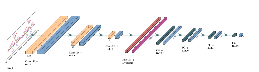
Figure 1: Architecture of the convolutional neural network (CNN) model, which as its input takes the $\mathcal{F}$-statistic atoms. The CNN is made up of a stack of three convolutional layers (labelled Conv1D in figure) followed by four fully connected layers (FC) and the output layer. The convolutional and fully connected layers all use the ReLU activation function. The convolutional part and the fully connected part of the network are separated by a flattening layer, needed to transform the output feature maps to a digestible input for the dense layers, and a dropout layer.

CNNs are a type of artificial neural networks that use convolutional layers as building blocks [51, 52]. While in fully-connected layers neurons are connected to all those of the previous layer, this would be computationally unfeasible for a high-dimensional input such as an image, for which a fully-connected layer would use a weight for each pixel. Convolutional layers avoid this problem by exploiting the spatial structure and repeating patterns in the data. To achieve this they convolve various independent filters (also called convolution kernels) with the input. Each filter is a matrix of weights to be trained, which slides along the input data, producing a feature map. These maps are then transformed through a non-linear activation function. This way, each filter learns to identify a pattern or characteristic of the data, regardless of location, which is preserved in the feature maps. These maps are then stacked to yield the input for the next layer. This enables the CNN to learn where features, or mixtures of features, are located in the data.

For this work we use a simple CNN, made up of three one-dimensional convolutional layers. This means that in each layer the filters slide along the time dimension (vertical axis) and convolve all columns at once. We always set the filter size to 3 along the time dimension in each layer, and to increasingly narrow down important features we use a decreasing number of 128, 64 and 8 independent filters per layer and set the stride parameter to 3, 2 and 1 respectively. The stride is the number of pixels the filter moves while sliding through the input matrix, i.e. the bigger the stride, the smaller the output feature maps. We do not implement pooling layers [53], since we find that for our particular architecture they are detrimental to the performance of the network.

The convolutional layers are then followed by a flattening and dropout layer [54] and four fully-connected layers. Again we decrease the number of neurons from layer to layer (256, 128 and 64) so that the number of trainable parameters decreases when approaching the final output. The last of the fully-connected layers gives the output of the network. We choose this to be a single continuous, positive value $\rho_{\textrm{CNN}}$ which we train to match the injected SNR from Eq. (9) for each sample in the signal training set, and to return 0 for pure-noise samples. We use the Rectified Linear Unit (ReLU) activation function [55] for all layers, including for the output, which produces the desired range of values for an SNR-like quantity: $\rho_{\textrm{CNN}}\in[0,+\infty)$. The dropout layer, which helps to prevent the CNN from overfitting [54], has a dropout rate of $0.33$.

The full network architecture is illustrated in Fig. 1 and has been implemented using the Keras library [56] based on the Tensorflow infrastructure [57]. For the various hyperparameters, we chose starting values from an exploratory run with the optimization framework Optuna [58], minimizing the loss on the validation set using a sampler based on the Tree-structured Parzen Estimator algorithm [59], and further tuned them manually.

III.3 Training strategy

The CNN is trained by minimizing a loss function $L$ over a training set containing both pure-noise samples and simulated signals. We use the mean squared error loss:

$$L=\frac{1}{n}\sum_{i=1}^{n}(\rho_{\textrm{inj}}-\rho_{\textrm{CNN}})^{2}\,,$$ (10)

where $\rho_{\textrm{inj}}$ is the injected SNR of the training signals, corresponding to Eq. (9). The training of our CNN’s continuous output function can therefore be considered a regression learning approach.

In general, we separate the training into two stages which differ with respect to the injection set (both in the number of training samples and the SNR range of signal samples), optimizer and number of epochs. A summary of the parameters used in each stage are shown in Tab. 2 and will be explained in more detail below.

When training a network, the weights are updated by an optimizer through gradient descent. There is a variety of well-established optimizers built to e.g. prioritize speeding up convergence or improving generalization. We use the Adam optimizer [60] in a first training stage, i.e. for the first 200 epochs, and the Stochastic Gradient Descent algorithm (SGD) [61] for the remaining 1000 epochs. We found that the Adam algorithm converges rapidly while the SGD generalizes better, reducing the unwanted effect of overfitting [62].

We also use the curriculum learning (CL) training strategy [63]. CL has been applied on GW data in previous works [64, 65] and consists of training on datasets of increasing difficulty. The difficulty criterion depends on the type of data and problem, and for our case we choose the range of injected SNRs. We use a simple two-stage CL strategy, first training on an easier dataset with strong signals (high SNR) and then adding a more difficult dataset, i.e. weaker signals. We align the stages of CL to the change in optimizer. More details on the training sets are given in Sec. III.4. Alternative CL approaches avoid re-using the easier dataset in further stages, but we decide to keep it also in the final stage so that the model still remains robust to the stronger signals.

We train two CNN models with the same architecture, the same CL setup, etc.: one on only-rectangular signals and one on only-exponential signals. All training sets are equally split into noise and signal atoms. The validation set, used to compute the loss function after each epoch, is $33\%$ of the training data.

		CL stage 1	CL stage 2
injection	$\rho_{\textrm{inj}}$	$U[6,40]$	$\textrm{set}\,1+U[4,10]$
set	$N_{\textrm{train}}$	$4\times 10^{4}$	$\textrm{set}\,1+6\times 10^{4}$
optimizer		Adam	SGD
epochs		200	1000

Table 2: Parameters used for the two stages of curriculum learning (CL). We first train on strong signals with $\rho_{\textrm{inj}}$ randomly drawn from a uniform distribution $U[6,40]$, and then we add to the training weaker signals with $\rho_{\textrm{inj}}$ randomly drawn from $U[4,10]$. The number of samples we train on is $4\times 10^{4}$ in the first CL stage, and during the second CL stage we add $6\times 10^{4}$ more samples, this time with $\rho_{\textrm{inj}}$ in the weaker range. The final stage uses the full $10^{5}$ samples training dataset, including both high-SNR and low-SNR signals. The $\{t^{0},\tau\}$ parameter ranges of the signals match the ones used for the search, which are listed in Tab. 1.

We start by training and testing on simulated Gaussian noise only, but with realistic gaps matching those of the O2 run (results will be shown in Sec. V.1). Real data, however, can present instrumental artifacts which differ from a Gaussian background. For tCW searches in particular, the disturbances that most affect them are narrow spectral features similar to quasi-monochromatic CWs or tCWs (so called “lines”) [66, 67, 68]. We also test these CNNs on real data (Sec. V.2). But as we will see, to be robust to non-Gaussianities of the data one must use real data also in the training set. There are different approaches that can be employed, e.g. only using real data in the training set, or using a mixture of both simulated and real data. We explain our choice and show our results in Sec. V.3.

III.4 Training sets

III.4.1 Gaussian-noise synthetic data

For Gaussian noise training data, we use the approach of generating “synthetic” detection statistics (and atoms, see appendix A.4 of Ref. [12]), which avoids generating and analyzing SFT files and therefore is considerably faster than full searches over simulated Gaussian noise data. Specifically, we use the synthesize_TransientStats program from LALSuite which draws samples of the quantities needed to compute atoms, either under the pure Gaussian noise assumption or as expected for signals (with randomized parameters) in Gaussian noise. It then produces the atoms we need as input for the CNNs and also the $2\mathcal{F}_{\textrm{max}}$ and $B_{\mathrm{tS}/\mathrm{G}}$ statistics (for given transient parameter search ranges) we will use for comparing the detection performance of the CNNs.

In each stage of the CL, the training set is balanced, with half of the samples being pure noise and the other half containing tCW signals. All signals correspond to Vela’s sky location. Frequency and spindowns do not matter for the synthesizing method. The parameters $\cos\iota$, $\psi$, and $\phi_{0}$ are randomized over their natural ranges, i.e. $\cos\iota\in[-1,1],\psi\in[0,\pi/2],\phi\in[0,2\pi]$. The transient parameters of the signals are drawn from the search ranges shown in Tab. 2, which also summarizes the SNR ranges and set sizes for the two CL levels.

III.4.2 Real data

The real-data training set atoms are generated from analyzing a $0.1$ Hz band of LIGO O2 data [40, 42]. To avoid training bias, we have to choose this band as disjoint from the search band around the nominal GW frequency of Vela, but it should be close enough to have similar noise characteristics. We center this band around $22.2$ Hz, which yields a frequency region without visible lines in the PSDs of the two detectors.

The noise samples are produced by running a grid-based search with PyFstat [38, 69] and storing the output atoms, using the same setup as in Tab. 1 except for the shift in frequency and using a coarser frequency resolution to reduce correlations between atoms at different $\lambda$: namely $df=5\times 10^{-6}$ Hz for the first CL stage and $df=3\times 10^{-6}$ Hz for the second.

The signal samples of this training set are generated by injecting signals at random frequencies within the same offset band, with spindowns fixed to the nominal GW values (twice those from pulsar timing). Atoms are then produced by a single-template PyFstat analysis for each injection.

III.5 Timings

The training of the network takes about $1.8$ hours on a Tesla V100-PCIE-32GB for only synthetic data. When including real data, the training takes twice as long in total. After training, evaluation on the same GPU takes $c_{\textrm{CNN}}\approx 4\times 10^{-4}$ s per sample, when averaged over a batch of $10^{4}$ samples using Tensorflow’s method Model.predict_on_batch. This compares favorably with costs for the $2\mathcal{F}_{\textrm{max}}$ or $B_{\mathrm{tS}/\mathrm{G}}$ statistics, which for the same set of transient parameters take $\approx 10^{-2}$ s per sample for rectangular windows (similar with both the LALSuite CPU code on a Intel Xeon Gold 6130 2.10GHz and the PyFstat GPU version from Ref. [39] on the same V100) and for exponential windows over 15 s on the CPU and $c_{B_{\mathrm{tS}/\mathrm{G}}^{\textrm{e}}}^{\textrm{GPU}}\approx 3\times 10^{-2}$ s on the V100.

IV Evaluation method

The output $\rho_{\textrm{CNN}}$ can be used as a detection statistic for hypothesis testing. We compare the performance of the CNNs with other detection statistics using receiver operating characteristic (ROC) curves on the separate test sets described below. These show the probability of detection $p_{\textrm{det}}$, corresponding to the fraction of signals above threshold, or true positives, as a function of the probability of false alarm $p_{\textrm{FA}}$, which is equal to the fraction of false positives from pure-noise samples. The number of noise samples determines how deep in $p_{\textrm{FA}}$ the curves can go, while the number of signal samples determines the accuracy of the $p_{\textrm{det}}$ estimate. In the following we always use $\approx 10^{7}$ noise samples and $10^{4}$ signal samples. The latter corresponds to $p_{\textrm{det}}$ uncertainties of $\lesssim 2\%$, and we will consider differences in ROC curves below this level as marginally significant. This disparity in noise and signal set sizes is due to the fact that, as mentioned in Sec. II, typical template bank sizes for standard searches can reach the order of millions, and so the operating $p_{\textrm{FA}}$ at which we assess the performance of our method must reach at least $10^{-6}$ to $10^{-7}$.

We will compare two versions of the CNN, one trained on only rectangular windows (output $\rho_{\textrm{CNN}}^{\textrm{r}}$) and the other trained on only exponential windows (output $\rho_{\textrm{CNN}}^{\textrm{e}}$), with the detection statistics $2\mathcal{F}_{\textrm{max}}$ and $B_{\mathrm{tS}/\mathrm{G}}$. We also use the r/e superscripts on these statistics depending on the window assumed in their computation. In addition, in this section we introduce a two-stage filtering process combining a CNN with $B_{\mathrm{tS}/\mathrm{G}}$.

IV.1 Testing sets

Our test sets are constructed to match the O2 Vela search discussed in Sec. II.3. For both the synthetic and real data case, we generate two separate test sets: both with the same $10^{7}$ noise samples, corresponding to the number of $\lambda$ parameters in the template bank for our reference search (compare Tab. 1). But the $10^{4}$ signal samples are rectangular-shaped for the first set, and exponentially-decaying-shaped for the second. The generation methods for each set are the same as described in Sec. III.4. The transient parameter ranges of the signal testing set are the same as those of the training sets, while the $\rho_{\textrm{inj}}$ of the testing sets are drawn from $U[4,40]$. The real data signal frequencies are randomly drawn from a $0.1$ Hz band around the nominal GW frequency of Vela.

Figure 2: Flowchart of three different methods for the tCW search: from the SFT data to $\mathcal{F}$-statistic atoms and then either via partial sums and marginalization to the $B_{\mathrm{tS}/\mathrm{G}}$ statistic, or to the CNN. In the two-stage filtering method, after the CNN a subset of candidates get passed back to the branch leading to $B_{\mathrm{tS}/\mathrm{G}}$. (For “synthetic” data, one starts directly from atoms.)

IV.2 Two-stage filtering

We have seen in Sec. III.5 that evaluating the CNNs is very fast. In particular, for exponential windows it is faster than even the GPU implementation of $2\mathcal{F}_{\max}^{\,\textrm{e}}$ and $B_{\mathrm{tS}/\mathrm{G}}^{\textrm{e}}$ from Ref. [39]. Motivated by this, in all of the following tests we also evaluate a combined detection approach, using the CNN as a preliminary filter stage with $B_{\mathrm{tS}/\mathrm{G}}$ as a second stage. The CNN can first be run on all the available data, and then a follow-up with the traditional detection statistic is done only if $\rho_{\textrm{CNN}}$ is above a given threshold. A simplified flowchart of this method, in comparison with the purely traditional and the pure CNN approaches, is shown in Fig. 2.

The amount of follow-up candidates can be set by choosing an operating $p_{\textrm{FA}}^{\textrm{CNN}}$ for the CNN stage, so that we gain as much sensitivity as possible while the whole pipeline is still computationally less expensive than directly computing $B_{\mathrm{tS}/\mathrm{G}}$ over all templates.

Towards low overall $p_{\textrm{FA}}$, we will see that performance improves compared to the single-stage CNN and approaches that of the pure $B_{\mathrm{tS}/\mathrm{G}}$ more closely. It is also possible for this two-stage method to achieve higher $p_{\textrm{det}}$ at low $p_{\textrm{FA}}$ than pure $B_{\mathrm{tS}/\mathrm{G}}$ if the CNN learns to better discard some noise features that would cause loud $B_{\mathrm{tS}/\mathrm{G}}$ outliers. On the other hand, the ROC curves of this method will not arrive at the point $(p_{\textrm{det}}=1,p_{\textrm{FA}}=1)$ as is normally the case for single-stage detection methods. Any signals lost, i.e. the amount of $p_{\textrm{det}}$ lost, during the first stage cannot be restored, since only the candidates passing that stage’s threshold are passed on to $B_{\mathrm{tS}/\mathrm{G}}$. Therefore, by choosing a particular $p_{\textrm{FA}}^{\textrm{CNN}}$, the highest probability of detection the two-stage method can reach will be at most $p_{\textrm{det}}^{\textrm{CNN}}(p_{\textrm{FA}}^{\textrm{CNN}})$.

We choose $p_{\textrm{FA}}^{\textrm{CNN}}=10^{-3}$ as an operating point, since it offers a good compromise between computational cost for the follow-up and the loss of overall $p_{\textrm{det}}$ at that operating point, as we will see in Sec. V.1.

In the case of an exponential window test set with $N\approx 1.15\times 10^{7}$ templates and with the hardware and timings as in Sec. III.5, the first stage takes $c_{\textrm{CNN}}\times N\approx 1.3$ hours. We pass a fraction of $10^{-3}$ of candidates to the second stage where $B_{\mathrm{tS}/\mathrm{G}}^{\textrm{e}}$ is evaluated. This is then expected to take $c_{B_{\mathrm{tS}/\mathrm{G}}^{\textrm{e}}}^{\textrm{GPU}}\times p_{\textrm{FA}}^{\textrm{CNN}}\times N\approx 350$ s. The two-stage filtering method thus takes in total less than $1.5$ hours against the $c_{B_{\mathrm{tS}/\mathrm{G}}^{\textrm{e}}}^{\textrm{GPU}}\times N\approx 95$ hours needed without the first CNN stage. A single-stage $B_{\mathrm{tS}/\mathrm{G}}^{\textrm{e}}$ search on a CPU (Intel Xeon Gold 6130 2.10GH) would even take $\gtrsim 4\times 10^{4}\,$hours.

V Performance on synthetic and real data

V.1 Results on synthetic data

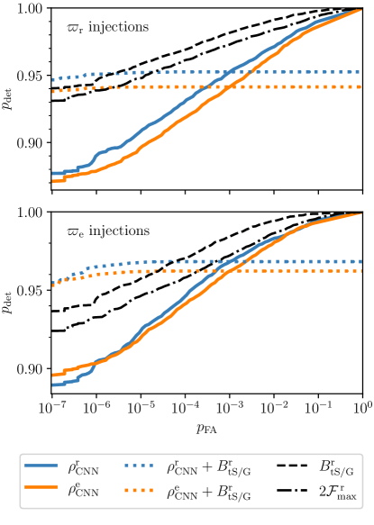
Figure 3: ROC curves with synthetic data as testing set and CNNs trained on synthetic data. Note the vertical axis is zoomed in. Both panels use the same noise testing set, but the signals in the testing sets are rectangular-windowed in the upper panel, and exponentially decaying in the bottom panel. For both panels, the black lines are the ROC curves for $2\mathcal{F}_{\max}^{\,\textrm{r}}$ (dash-dotted) and for $B_{\mathrm{tS}/\mathrm{G}}^{\textrm{r}}$ (dashed), always searching for a rectangular signal (even when the test set contains exponentially decaying signals). The solid windowed lines are the ROC curves for the CNNs, trained on only rectangular-shaped signals (blue) and on onlys exponentially decaying signals (orange). The dotted colored lines are the ROC curves for the two-stage filtering method, with the corresponding windows used in training.

We start by testing the CNNs that were trained on synthetic data only, also using purely synthetic data for the test. As mentioned in Sec. III.4.1, synthetic data are random draws of the $\mathcal{F}$-statistic atoms, assuming an underlying Gaussian noise distribution, from which the tCW detection statistics $2\mathcal{F}_{\max}^{\,\textrm{r}}$ and $B_{\mathrm{tS}/\mathrm{G}}^{\textrm{r}}$ can then be calculated. The detection problem is easier for this case than for real data, so we show these results as a starting point. In Fig. 3 we show ROC curves comparing the CNNs against the other two detection statistics. The two subplots refer to the two different test sets, which differ only in the window function of the injected signals, but for both cases the standard detection statistics use rectangular windows.

As expected [12], $B_{\mathrm{tS}/\mathrm{G}}^{\textrm{r}}$ performs marginally better than $2\mathcal{F}_{\max}^{\,\textrm{r}}$. Both their probabilities of detection surpass $p_{\textrm{det}}=90\%$ even at $p_{\textrm{FA}}$ as low as $10^{-7}$. The two CNNs (trained on only rectangular and only exponentially decaying windows) perform similarly overall, with at most $\lesssim 1\%$ difference in $p_{\textrm{det}}$ between each other and a loss with respect to $B_{\mathrm{tS}/\mathrm{G}}^{\textrm{r}}$ of at most $7\%$ for rectangular and $5\%$ for exponential windows.

The two-stage filtering reaches a plateau at higher $p_{\textrm{FA}}$ values, corresponding (as mentioned in Sec. IV.2) to the fixed ($p_{\textrm{FA}}=10^{-3},p_{\textrm{det}}<1)$ operating point of the first stage of the method. However, at low $p_{\textrm{FA}}$ it considerably improves $p_{\textrm{det}}$ for both CNNs. It actually performs marginally better than $B_{\mathrm{tS}/\mathrm{G}}^{\textrm{r}}$ below $p_{\textrm{FA}}<10^{-5}$ for both types of signals: by $\approx 1$% for rectangular and $\approx 2$% for exponentially decaying injections.

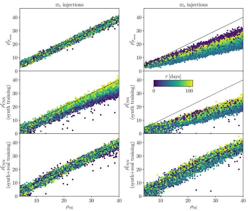
Figure 4: Estimated SNRs from three different methods (one for each row) as a function of injected SNRs in real LIGO O2 data. From top to bottom, the estimated SNRs are $\rho_{\mathcal{F}_{\max}}^{\,\textrm{r}}$ estimated from $2\mathcal{F}_{\max}^{\,\textrm{r}}$, in the second row $\rho_{\textrm{CNN}}^{\textrm{r/e}}$ is estimated from the CNNs trained on only synthetic data with windows matching that of the test set and lastly, in the third row $\rho_{\textrm{CNN}}^{\textrm{r/e}}$ is estimated from the CNNs trained on both synthetic and real data. The injected signals are rectangular-shaped on the left column and exponentially decaying on the right column. The color scale (shared between all panels) indicates the durations of the injected signals. For guidance, we always plot the diagonal of the subplots, where ideally the points should align.

The improvement is not necessarily significant compared with counting uncertainty, and in the exponential case where it seems larger we have also not compared to the traditional statistics using exponential windows. Still, in general such an improvement is indeed possible because $B_{\mathrm{tS}/\mathrm{G}}$ is not an optimal statistic in either case. As discussed in Ref. [34] (for CWs), a better detection statistic for a given signal population can in general be obtained by marginalization over an appropriate amplitude prior, as opposed to the unphysical prior that the maximization used for the $\mathcal{F}$-statistic (and derived statistics such as $2\mathcal{F}_{\textrm{max}}$ and $B_{\mathrm{tS}/\mathrm{G}}$) corresponds to. In addition, Ref. [70] has demonstrated how in particular for short data stretches a more sensitive statistic than the standard $\mathcal{F}$-statistic can be constructed, mainly exploiting a reduction in noise degrees of freedom. Therefore, it seems consistent that a CNN can also learn to behave better than the standard statistics, and more similarly to the improved alternatives, in at least certain parts of the tCW parameter space.

V.2 Results of synthetic-trained CNNs on real data

In the previous section we have shown how CNNs can be used as a competitive method against the standard detection statistics, at least in the context of synthetic data. We now evaluate the same models trained with synthetic data, but now we test on real data. The corresponding CNN detection probabilities suffer additional losses, compared to Fig. 3, of up to $7\%$ and $16\%$ for rectangular and exponential windows respectively. Instead of showing these ROC curves, we proceed directly to identifying and addressing the main reason for these losses.

For real-data injections, we show in Fig. 4 the estimated $\rho_{\textrm{CNN}}$ compared with the traditional estimator [33]

$$\rho_{\mathcal{F}_{\max}}^{\textrm{r}}=\sqrt{2\mathcal{F}_{\textrm{max}}^{\,\textrm{r}}-4}\,,$$ (11)

both as functions of $\rho_{\textrm{inj}}$. Different injection windows are covered in the two columns. Ideally, each estimator would align all the points on the diagonals of these plots.

We see that $\rho_{\mathcal{F}_{\max}}^{\textrm{r}}$ (first row) aligns well with the injected $\rho_{\textrm{inj}}$ for rectangular windows, but for exponentially decaying signals there is a loss in recovered SNR (i.e. the points do not align with the diagonal) because the injected window (exponential) and the search window (rectangular) do not match. The loss in SNR is also enhanced by a 12-day gap in the data, which we discuss in more detail in Appendix B.

In the second row, we see that the CNN trained on synthetic data and rectangular windows recovers $\rho_{\textrm{CNN}}^{\textrm{r}}$ that mostly align with $\rho_{\textrm{inj}}$, but the loss increases as the duration of the injected signal decreases. The loss in SNR is even more evident for $\rho_{\textrm{CNN}}^{\textrm{e}}$ on exponentially decaying signals. Since both of these CNNs were trained on synthetic data only, it is natural to expect that they are not robust to detector artifacts that could contaminate the data, especially at shorter durations [71, 68]. We will now demonstrate that it helps to include real data in the training set to mitigate this effect.

V.3 Performance of training on real data

Figure 5: ROC curves with real data as the testing set and CNNs trained on both synthetic and real data. Note the vertical axis is zoomed in. Both panels use the same noise testing set, but the test signals are rectangular-shaped in the upper panel, and exponentially decaying in the bottom panel. The legend structure is the same as in Fig. 3, with the addition of two extra ROC curves in the exponential test case corresponding to the $2\mathcal{F}_{\max}^{\,\textrm{e}}$ and $B_{\mathrm{tS}/\mathrm{G}}^{\textrm{e}}$ statistics computed with the more expensive exponential window.

To improve sensitivity, we also trained CNNs using real data, keeping the same architecture. As mentioned before in Sec. III.3, there are different ways one can incorporate real data in the training set. We have tried different implementations using the same total number of training epochs: training a model from scratch on only real data, training a model on a mixture of synthetic and real data, and taking the previous synthetic-only-trained model and continuing its training on only real data (similar to a CL approach).

We find that training exclusively on real data yields a good signal recovery, i.e. removes the SNR losses seen in Fig. 4, but overestimates the SNR of the noise samples, leading to inferior ROC results overall. This effect is mitigated when training with both synthetic and real data. Between the two options of training on a mixture of both all at once, and first training on synthetic and then on real data, the latter performs best. More precisely, when first training on synthetic and then on real data, we take the previously trained CNNs on synthetic data for 200+1000 epochs (first CL stage + second CL stage) and continue their training on only real data for another 200+1000 epochs.

As before, we train two models, each on a single window type. In the third row of Fig. 4 we show the recovered $\rho_{\textrm{CNN}}^{\textrm{r/e}}$ from these networks (trained first on synthetic and then real data) on real-data injections. For rectangular injections, the loss in SNR is now reduced compared to the CNNs with only synthetic training data. The issue of more SNR loss for shorter signals is largely resolved except for a few underestimated outliers with short durations: the CNN is now able to recover both long and short signals well. In the exponential case, $\rho_{\textrm{CNN}}^{\textrm{e}}$ also aligns well with the injected $\rho_{\textrm{inj}}$, with just a wider scatter.

The models trained on both synthetic and real data also perform well on real noise samples, not producing overly loud outliers. ROC curves for this case are shown in Fig. 5. For rectangular signals, sensitivities of all the different statistics are quite similar to those on synthetic data (top panel of Fig. 3). However, while for synthetic data the two-stage filtering performance matched or exceeded that of the standard detection statistics at low $p_{\textrm{FA}}$, it now shows a marginal loss in the same regime with respect to the standard statistics, but of only $\approx 1\%$.

Also, the CNN trained on exponential windows performs marginally better even with rectangular window injections at the lowest values of $p_{\textrm{FA}}$. It was noted by Ref. [12] that also $2\mathcal{F}_{\max}^{\textrm{\,e}}$ can outperform $2\mathcal{F}_{\max}^{\textrm{\,r}}$ on rectangular signals. However, without larger studies on different configurations and data sets it cannot be determined if the observed phenomenon in the CNNs is related or just due to specifics of the training and test data sets.

On the other hand, for the exponential test set, $p_{\textrm{det}}$ for all statistics has systematically worsened by $10\%$ to $15\%$ compared to the synthetic results from Fig. 3. This could be because the weak late-time portions of the signals are more difficult to pick up in real noise. The CNNs lose relatively less detection power, meaning that the gap in $p_{\textrm{det}}$ against the traditional statistics has narrowed down: at the lowest $p_{\textrm{FA}}$, the difference in $p_{\textrm{det}}$ between $B_{\mathrm{tS}/\mathrm{G}}^{\textrm{r}}$ and $\rho_{\textrm{CNN}}^{\textrm{e}}$ is down to $3\%$.

Since this is our most complete test set, we also show the results of the more computationally expensive statistics computed with windows matching the injections, i.e. $2\mathcal{F}_{\max}^{\,\textrm{e}}$ and $B_{\mathrm{tS}/\mathrm{G}}^{\textrm{e}}$. To obtain these we used the GPU implementation from Ref. [39]. Their ROC curves improve by $2-3\%$ over the statistics with rectangular windows.

For $p_{\textrm{FA}}<10^{-5}$ the two-stage filtering ROC curve very closely matches that of $B_{\mathrm{tS}/\mathrm{G}}^{\textrm{e}}$. It cannot yield higher $p_{\textrm{det}}$ (as it did in the synthetic case) on this specific data set, because the template corresponding to the loudest $B_{\mathrm{tS}/\mathrm{G}}^{\textrm{e}}$ outlier also passes the first-stage $\rho_{\textrm{CNN}}^{\textrm{r/e}}$ threshold. But it does converge to the sensitivity of the traditional statistic when far enough to the left of the ROC to go below the plateau level set by the first stage. As discussed before, it also takes 80 times less time even with the GPU implementation of Ref. [39].

It is important to remember that ROC performance depends on the population of signal candidates considered. In this case we use signals with $\rho_{\textrm{inj}}\in[4,40]$. In Sec. VII we will revisit the same real-data noise set but with a different injection set matching the one used in Ref. [19] for establishing upper limits.

VI Parameter estimation with CNNs

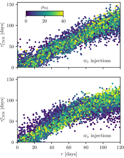
Figure 6: Duration parameters $\tau_{\textrm{CNN}}^{\textrm{r/e}}$ estimated by the two-output CNNs trained on rectangular (top panel) and exponential signals (bottom panel), plotted against the duration $\tau$ of the injected signal. These use the same synthetic test sets as in Sec. V.1, with windows matching the training in each panel. Only signals passing the $\rho_{\textrm{CNN}}^{\textrm{r/e}}$ thresholds of the two-stage filtering are plotted. The color scale (shared between both panels) corresponds to the $\rho_{\textrm{inj}}$ of the injected signals.

So far, we have considered a CNN with only one output: the estimated SNR, which only allows yes/no detection statements. In practice, one will also be interested in the parameters of a signal candidate. Estimates of the frequency-evolution parameters $\lambda$ are naturally obtained from where the detection statistic peaks in the template bank. In our preferred setup, the two-stage filtering, final candidates will additionally have $(t^{0},\tau)$ estimates from the algorithm in Ref. [12].

However, CNNs can also estimate multiple parameters directly. In this section, we present a first exploration of this possibility via training CNNs with multiple outputs. We keep the same architecture as before with only the addition of one extra node to the output layer: we now want to output both $\rho_{\textrm{CNN}}$ and a duration estimate $\tau_{\textrm{CNN}}$ for a potential signal. One could also estimate the starting time $t^{0}$ by adding another output, but since in our setup the starting time is limited to a small range around $T_{\textrm{gl}}$, we ignore it for this first proof of concept.

We here show the results of two newly trained models with the additional $\tau_{\textrm{CNN}}$ output and trained and tested with synthetic data. The duration input labels for training are normalized to a range between $[0,1]$. The output can then be transformed back to the duration in days. In general, we find that the accuracy of the $\rho_{\textrm{CNN}}$ estimation remains unaltered, while the quality of $\tau_{\textrm{CNN}}$ estimates depends on which type of windows we use in training. These are shown for one CNN trained on only rectangular signals and by one trained on only exponential signals, as functions of the injected durations from the test set, in Fig. 6. To focus on signals that are at least marginally detectable, we only include those passing the $\rho_{\textrm{CNN}}^{\textrm{r/e}}$ thresholds of the two-stage filtering, in both cases corresponding to $p_{\textrm{FA}}^{\textrm{CNN}}=10^{-3}$.

For the rectangular-trained CNN, the estimated durations $\tau^{\textrm{r}}_{\textrm{CNN}}$ follow quite well the true durations, but with some scatter especially for low-SNR signals. About 3% of signals form a set of outliers with durations underestimated by over 95%, mostly for shorter injections. Excluding these outliers, the remaining distribution of relative errors is well-centered around zero with a root-mean-square (RMS) of $27\%$. For the exponential-trained CNN, there is a mild trend towards more under-estimated $\tau^{\textrm{e}}_{\textrm{CNN}}$ values for longer injected signals. In this case, about 7% of signals are underestimated by over 95%, but after excluding this subset the error distribution is only slightly wider with a RMS of $29\%$.

We also tested these synthetic-trained CNNs on real data. For rectangular signals, the duration estimation is overall quite robust, and the plot equivalent to Fig. 6 follows the same shape except for some more cases of overestimation at high durations. The outlier percentages for real data estimations slightly increase to 6% and the RMS error stays close to 27%. For exponential signals, there is noticeably more overestimation and the outlier percentage increases to 11% and the RMS error to 47%.

As an additional investigation, we trained a two-output CNN on signals with both rectangular and exponential windows. Overall it behaves like a mixture of the results of the two separately trained networks, with the exception of stronger overestimation at long durations and high SNRs in real data. Performance could potentially be improved by adding another output acting as a window label, since the duration parameter $\tau$ actually has different meanings for the two different windows, as also discussed in Ref. [14]. This would be similar to how Ref. [12] has already discussed treating window function choice as an additional parameter in Bayesian parameter estimation.

This and other possible improvements to the architecture and training of the two-output network to obtain better accuracy, and any further extensions of this approach to parameter estimation with CNNs, are left for future work.

VII O2 Vela glitch upper limits

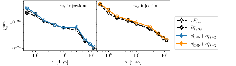
Figure 7: Upper limits on $h_{0}$ as a function of duration $\tau$ for the different methods: $2\mathcal{F}_{\max}^{\,\textrm{r}}$ (dash-dotted black) and $B_{\mathrm{tS}/\mathrm{G}}^{\textrm{r}}$ (dashed black), both recovering rectangular signals. The two different shapes of the injections are used in the different panels (rectangular on the left, exponential on the right). In each subplot we also show the two-stage filtering trained on only rectangular-shaped signals (left panel, solid blue) and two-stage filtering trained on only exponentially decaying signals (right panel, solid orange).

No detection of a post-glitch tCW signal was reported in the O2 search [19], so upper limits on the GW strain amplitude were set. Having found no interesting outliers in the CNN results on the same data set either, we repeat the procedure here, but covering both rectangular and exponential window choices.

Upper limits are computed by injecting simulated signals in the same data used in the search and then counting how many signals are recovered by the chosen method. For a set of injections at fixed duration $\tau$, one can then fit a sigmoid curve of the counts against injected amplitude $h_{0}$ to find the upper limit amplitude $h_{0}^{90\%}$ at which $90\%$ of the injected signals are recovered above the threshold of each statistic. A more detailed explanation can be found in the appendix of Ref. [19].

As the thresholds to distinguish between noise and signal candidates we use the highest output of the search over the original data and the ranges given in Table 1, for each detection statistic. This means that the thresholds of the different detection statistics do not necessarily correspond to the same $p_{\textrm{FA}}$, but it is a consistent method that can be applied to any statistic. It is also a conservative choice in the sense that any lower threshold would produce stricter upper limits, but would require outlier followup. In the special case of the two-stage filtering, the first threshold on the CNN stage is chosen to let a fraction $10^{-3}$ of candidates pass and the final threshold is given by the highest $B_{\mathrm{tS}/\mathrm{G}}$ in that remaining set.

We create an injection set with simulated signals of amplitude $h_{0}$ in the ranges used in the O2 search [19], chosen to correspond to detection statistics around the threshold values. This translates to mostly weaker signals compared to the test sets described in Sec. IV and used for the ROC curves in Sec. V. The durations of the injections are not distributed uniformly as done for the previous testing sets, but rather chosen at discrete steps from 0.5 to 120 days.

In Fig. 7, we reproduce the plot from Ref. [19] for rectangular-window signals, showing the upper limits on $h_{0}^{90\%}$ as a function of the duration parameter $\tau$, and we extend it with an exponential-window injection set. We show upper limits derived from several methods discussed before, namely $2\mathcal{F}_{\max}^{\,\textrm{r}}$, $B_{\mathrm{tS}/\mathrm{G}}^{\textrm{r}}$, and the two-stage filtering method using CNNs trained on only rectangular windows or only exponential windows, combined with $B_{\mathrm{tS}/\mathrm{G}}^{\textrm{r/e}}$. The statistics $2\mathcal{F}_{\max}^{\,\textrm{e}}$ and $B_{\mathrm{tS}/\mathrm{G}}^{\textrm{e}}$ for the full injection set are again omitted due to computational cost.

The upper limits from $2\mathcal{F}_{\max}^{\,\textrm{r}}$ using rectangular injections can be directly compared to those obtained in Ref. [19]. They are consistent within $1\sigma$ error bars, and the small differences are due to the different individual injections and the different sigmoid fitting procedure and uncertainty estimation (matching the implementation as in Ref. [20]).

The upper limits from the two-stage filtering reach values close to $2\mathcal{F}_{\max}^{\,\textrm{r}}$ and $B_{\mathrm{tS}/\mathrm{G}}^{\textrm{r}}$, higher only by 6–7% for both signal types.

As seen before in the real-data ROC curves, the two-stage filter cannot improve over $B_{\mathrm{tS}/\mathrm{G}}^{\textrm{r/e}}$ on these specific data sets because the templates corresponding to the loudest outliers from those statistics also pass the first-stage $\rho_{\textrm{CNN}}^{\textrm{r/e}}$ thresholds.

Another factor that could potentially be relevant in this new, typically weaker injection set, is that upper limits depend strongly on the performance for weak signals near threshold, which are the most challenging for CNNs. This is exacerbated by using steps in the amplitude $h_{0}$, instead of SNR, to quantify the strength of the signals. While the SNR takes into account the other parameters that affect detectability, especially the inclination $\cos\iota$, the amplitude does not contain this information and so cannot be used as a direct proxy for the SNR. Therefore, at each $h_{0}$ step of the injection set, there can be a tail of signals with low SNRs, where the differences between the CNN and traditional detection statistics are more significant.

VIII Conclusions

In this work we present a new method based on CNNs for detecting potential tCWs – long-duration quasi-monochromatic GW signals – from glitching pulsars. CNNs have proven to be promising tools for detecting various GW signals, but have not been tested before on tCWs from glitching pulsars. Previous searches were entirely matched-filtering based and limited in computational cost. In this work we have used intermediate matched-filter outputs (the $\mathcal{F}$-statistic atoms) as input to the CNNs, which allows to replace the most computationally expensive part of the analysis. In particular, practical searches with the $2\mathcal{F}_{\textrm{max}}$ and $B_{\mathrm{tS}/\mathrm{G}}$ statistics were limited to assuming constant amplitude (rectangular window) tCWs due to the much higher cost of other window functions, while with CNNs we can easily train on different windows.

The CNNs are constructed to output an estimator of SNR in the data. We have trained and tested CNNs for either rectangular or exponentially decaying windows, first on synthetic, Gaussian data, but with gaps corresponding to the timestamps of the LIGO O2 data after the Vela glitch of 2016. We use curriculum learning, i.e. first train on stronger and then also on weaker signals. Then we have tested these CNNs on the real LIGO data from O2 as previously analyzed in Ref. [19], and also trained with real data using the same architecture to improve the results. We find the best results when starting from the model we had trained on synthetic data and continuing its training on only real data.

We find that a simple implementation of such atoms-based CNNs already approaches within 10% of the detection probability at fixed false-alarm probability of the traditional detection statistics. As a CNN-based method that mostly closes this remaining gap, we propose a two-stage filtering method consisting of first applying the CNN to all signal templates and only passing candidates above a certain threshold on $\rho_{\textrm{CNN}}$ to the $B_{\mathrm{tS}/\mathrm{G}}$ statistic. For a real data test set containing injected signals of broad SNR range (from 4 to 40), the probabilities of detection at false-alarm probabilities as low as $10^{-7}$ are only $\lesssim 2\%$ lower than those of $B_{\mathrm{tS}/\mathrm{G}}$ for rectangular windows and 4% better for exponential windows. Comparing the computing time of the two-stage filtering with that of $B_{\mathrm{tS}/\mathrm{G}}$ for exponential signals using the GPU implementation of Ref. [39], we find that our method is $80$ times faster than evaluating the full data without the CNN stage.

We then use this new method to set updated observational upper limits on the GW strain amplitude $h_{0}$ after the O2 Vela glitch, with extended parameter space coverage including exponentially decaying signals. For this we make a separate injection set with signal parameters in the same ranges as in Ref. [19]. The upper limits from the two-stage filtering almost match those reached by the standard statistics, higher only by $\lesssim 7\%$.

Thanks to its computational efficiency, the CNN-based approach can be a competitive method for the overall tCW search effort that is also complementary to the reference method: if extended to more generic searches, it will help increase overall detection probability by extending discovery space while one can afterwards still brute-force evaluate the traditional detection statistics when interested in pushing for the deepest possible upper limits on individual targets.

Considering such further applications of CNNs to tCWs from glitching pulsars, we have here focused on a single target pulsar and data set, but the approach can be generalized to other targets or even unknown sky positions, either by training from scratch in each case or through transfer learning [72]. Due to the computational efficiency of both the training and evaluation phase, the two-stage filtering could thus be scaled up to broader searches covering a larger variety of targets than currently feasible with the standard methods, especially when wanting to include multiple amplitude evolution window options.

Also, since CWs can be obtained from the tCWs model by setting a rectangular window function to cover the entirety of the data, this method can easily be applied to persistent CW targeted searches. Our implementation of CNNs, however, was designed specifically to avoid the computationally expensive computation of partial sums of the $\mathcal{F}$-statistic atoms over all the combinations of the transient parameters, which does not concern CW searches.

Furthermore, one could go beyond the current configuration, in which we trained the CNNs on $\mathcal{F}$-statistic atoms, i.e. quantities computed during the matched filtering step. This still constrains the frequency evolution of the signal to be CW-like, but already allows for flexible amplitude evolution and significant speed-up compared to the traditional method, effectively allowing to search a wider parameter space at the same cost. A different approach would be to train a CNN (or different type of network) on spectrograms or the full timeseries strain data, which could allow searches for unmodeled tCWs both in frequency and amplitude evolution.

The major drawback would be that the amplitudes of tCW signals are expected to be very weak, with $h_{0}$ upper limits from O3 reaching $10^{-25}$ [20]. Such signals are too weak to be directly discernible, e.g. in time-frequency maps of the data. A study of using Fourier transforms of the data as input to a CNN to search for persistent CWs was done in Ref. [48], and a broader set of machine-learning strategies on SFTs was evaluated in a public Kaggle challenge [73]. Similar approaches could be applied to tCWs as well, but it will be a challenging problem, which we leave for future work. Despite not reaching the high sensitivities of purely matched filtering methods, these faster, generic searches could still extend the tCW science case by enabling the search for post-glitch GWs corresponding to more general glitch models and over larger parameter spaces, potentially leading to all-sky, all-time, all-frequency blind searches of tCWs.

Appendix A $\mathcal{F}$-statistic atoms

Here we will explain in more detail the procedure to obtain the $\mathcal{F}$-statistic atoms, and resulting detection statistics, as implemented in LALSuite [35] and PyFstat [38]. The general approach, as originally developed for persistent CWs, is documented in Ref. [33] though we also include here the modifications for transients following Ref. [12] and adjust some of the notation for convenience.

Detection statistics for (t)CW signals can be derived from the likelihood ratio between hypotheses about a data set $x(t)$. In particular, a Gaussian noise hypothesis $\mathcal{H}_{\textrm{G}}$ and a signal hypothesis $\mathcal{H}_{\textrm{tS}}$ can be written as

$$\mathcal{H}_{\textrm{G}}:x(t) =n(t),$$ (12)

$$\mathcal{H}_{\textrm{tS}}:x(t) =n(t)+h(t;\lambda,\mathcal{A},\mathcal{T}).$$ (13)

We have written this for a single frequency-evolution template $\lambda$, but it can be generalized by iterating over a template bank.

The likelihood ratio between the two hypotheses can then be analytically maximized [31, 34] over the amplitude parameters $\mathcal{A}$, yielding the $\mathcal{F}$-statistic. As introduced in Eq. (8), it depends on different combinations of the start times $t^{0}$ and duration parameters $\tau$. The implementation consists of computing per-SFT quantities, the “$\mathcal{F}$-statistic atoms”. When weighted with an appropriate window and summed up, these give the building blocks for $2\mathcal{F}(t^{0},\tau)$.

In particular, following Ref. [12], $2\mathcal{F}(t^{0},\tau)$ is computed from the antenna-pattern matrix and projections of the data onto the basis of the signal model from Eq. (7), both depending on a window function $\varpi(t^{0},\tau)$. The CW case corresponds to a rectangular window covering the full observation time.

The antenna-pattern matrix can be written in block-form:

$$\mathcal{M}_{\mu\nu}(t^{0},\tau)=\mathcal{S}^{-1}T_{\textrm{data}}\begin{pmatrix}\hat{A}&\hat{C}&0&0\\ \hat{C}&\hat{B}&0&0\\ 0&0&\hat{A}&\hat{C}\\ 0&0&\hat{C}&\hat{B}\end{pmatrix}$$ (14)

where $T_{\textrm{data}}\equiv N_{\textrm{SFT}}T_{\textrm{SFT}}$, $\mathcal{S}^{-1}\equiv\frac{1}{N_{\textrm{SFT}}}\sum_{X\alpha}S_{X\alpha}^{-1}$ and $\hat{A},\hat{B},\hat{C}$ are the independent components of the matrix given by

$$\hat{A}(t^{0},\tau) \equiv\sum_{X\alpha}\varpi^{2}(t_{\alpha};t^{0},\tau)\langle(\hat{a}^{X}_{\alpha})^{2}\rangle_{t},$$ (15)

$$\hat{B}(t^{0},\tau) \equiv\sum_{X\alpha}\varpi^{2}(t_{\alpha};t^{0},\tau)\langle(\hat{b}^{X}_{\alpha})^{2}\rangle_{t},$$

$$\hat{C}(t^{0},\tau) \equiv\sum_{X\alpha}\varpi^{2}(t_{\alpha};t^{0},\tau)\langle\hat{a}^{X}_{\alpha}\hat{b}^{X}_{\alpha}\rangle_{t}.$$

We have used here the same notation from Sec. II, i.e. the $X,\alpha$ indices run over detectors and SFTs, respectively. For compactness, we have suppressed the transient parameters on the right-hand side of Eq. (14).

These components are noise-weighted (indicated by the hat) such that for a function $z^{X}_{\alpha}$

$$\hat{z}^{X}_{\alpha}(t)\equiv\sqrt{w^{X}_{\alpha}}z^{X}_{\alpha}(t),\quad$$ (16)

with weights $w_{\alpha}^{X}\equiv S_{X\alpha}^{-1}/\mathcal{S}^{-1}$, and time-averaged (indicated by the brackets) such that

$$\langle z^{X}_{\alpha}\rangle_{t}\equiv\frac{1}{T_{\textrm{SFT}}}\int_{t^{\alpha}}^{t_{\alpha}+T_{\textrm{SFT}}}z^{X}_{\alpha}(t)dt.$$ (17)

The definitions of the antenna-pattern functions $a(t),b(t)$ can be found in Ref. [31]. In practice, $a^{X}_{\alpha}$ and $b^{X}_{\alpha}$ are computed once per SFT at its representative timestamp instead of computing the time averages explicitly, and noise-weighted afterwards.

The square root of the determinant of the matrix is then (suppressing again the $(t^{0},\tau)$ dependency):

$$\hat{D}\equiv\hat{A}\hat{B}-\hat{C}^{2}\,.$$ (18)

Note that we have assumed the long-wavelength limit approximation [75] which implies that $a(t),b(t)$ are real-valued and there are no off-axis terms in Eq. (14).

The SFT data is normalized as

$$y^{X}_{\alpha}(t)\equiv\frac{x^{X}_{\alpha}(f)}{\sqrt{\frac{1}{2}T_{\textrm{SFT}}S_{X\alpha}(f)}},$$ (19)

and used to define the two complex quantities

$$F_{\textrm{a},\alpha}^{X}\equiv\int_{t_{\alpha}}^{t_{\alpha}+T_{\textrm{SFT}}}y^{X}_{\alpha}(t)\hat{a}^{X}_{\alpha}(t)e^{-i\phi^{X}_{\alpha}(t)}dt,$$ (20)

$$F_{\textrm{b},\alpha}^{X}\equiv\int_{t_{\alpha}}^{t_{\alpha}+T_{\textrm{SFT}}}y^{X}_{\alpha}(t)\hat{b}^{X}_{\alpha}(t)e^{-i\phi^{X}_{\alpha}(t)}dt,$$

where $\phi_{\alpha}^{X}(t)$ is the phase obtained from integrating the frequency evolution of a given signal template. These quantities take the role of the data projections $x_{\mu}$ in the more abstract notation used earlier, with the detailed translation documented in Ref. [33].

The set of $\{\langle(\hat{a}^{X}_{\alpha})^{2}\rangle_{t},\langle(\hat{b}^{X}_{\alpha})^{2}\rangle_{t},\langle\hat{a}^{X}_{\alpha}\hat{b}^{X}_{\alpha}\rangle_{t},F_{\textrm{a},\alpha}^{X},F_{\textrm{b},\alpha}^{X}\}$ from equations (15) and (20) are what we refer to as the $\mathcal{F}$-statistic atoms. More technical detail of how these are implemented in LALSuite can be found in Ref. [33, 76], based on the algorithm by Ref. [77].

For the CNN, we use these atoms as input. On the other hand, to compute traditional detection statistics the codes compute Eq. (15) and Eq. (18) and

$$F_{\text{\{a,b\}}}(t^{0},\tau)\equiv\sum_{X\alpha}\varpi(t_{\alpha};t^{0},\tau)F^{X}_{\text{\{a,b\}},\alpha},$$ (21)

i.e. the window-weighted partial sums of the atoms. Finally, from all of these it then computes

$$2\mathcal{F}(t^{0},\tau)=\frac{2}{\hat{D}}[\hat{B}|F_{\textrm{a}}|^{2}+\hat{A}|F_{\textrm{b}}|^{2}-2\hat{C}\mathfrak{R}(F_{\textrm{a}}F_{\textrm{b}}^{\ast})].$$ (22)

This still depends on $(t^{0},\tau)$, through the implicit partial sums for all quantities on the right-hand side.

For a search over unknown transient parameters, one can discretize the ranges $t^{0}\in[t^{0}_{\textrm{min}},t^{0}_{\textrm{min}}+\Delta t^{0}]$ and $\tau\in[\tau_{\textrm{min}},\tau_{\textrm{min}}+\Delta\tau]$ in steps $dt^{0}$ and $d\tau$. Then, $\mathcal{F}_{mn}\equiv\mathcal{F}(t^{0}_{m},\tau_{n})$ is computed for a $N_{t^{0}}\times N_{\tau}$ rectangular grid

$$t^{0}_{m} =t^{0}_{\textrm{min}}+mdt^{0},$$ (23)

$$\tau_{n} =\tau_{\textrm{min}}+nd\tau.$$

Finally, one can e.g. maximize over $\{t^{0},\tau\}$, obtaining the detection statistic $2\mathcal{F}_{\textrm{max}}$, or alternatively marginalize over them, obtaining the transient Bayes factor $B_{\mathrm{tS}/\mathrm{G}}$. Complete derivations of both these detection statistics for tCWs can be found in Ref. [12]. They still depend on the frequency evolution parameters $\lambda$, and a search where the source parameters are not exactly known will typically consist of setting up a grid in $\lambda$ covering the desired range.

As described in Ref. [39], the pycuda GPU implementation in PyFstat is largely equivalent to the one in LALSuite. (For CPU calculations of the transient $\mathcal{F}$-statistic and other functionality, PyFstat calls LALSuite functions through SWIG wrappings [74].) However, when testing for this paper, we noticed that a LALSuite fix that was introduced in 2018 had not been included in PyFstat yet: when computing $\mathcal{F}_{mn}$ over very little data (few SFTs from a single detector), the antenna-pattern matrix can become ill-conditioned for some combinations of $\lambda$ parameters, making the determinant from Eq. (18) approach zero and causing spuriously large detection statistics outliers. PyFstat 2.0.0 (yet to be released as of this writing) avoids this problem the same way as the LALSuite code, by truncating to $2\mathcal{F}_{mn}=4$ (the Gaussian noise expectation value) when the antenna-pattern matrix condition number exceeds a threshold that has been fixed to $10^{4}$ . Results included in Sec. V use this version. This issue of the $\mathcal{F}$-statistic for short durations has also been described in Ref. [70], where an alternative and improved statistic was derived for this case.

Appendix B The effect of gaps on traditional detection statistics

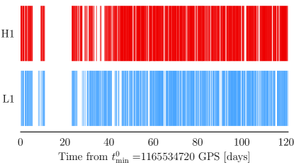
Figure 8: Time segments of the two LIGO detectors H1 and L1 corresponding to the data analyzed in this work. For reference the Vela 2016 glitch happened at $T_{\textrm{gl}}=1165577920\,$GPS, corresponding to 0.5 days on this scale.

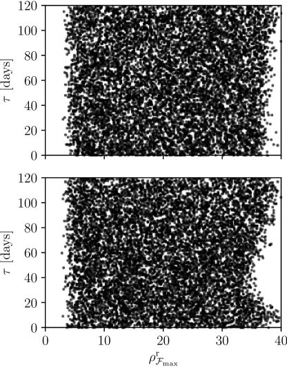
Figure 9: Duration parameters for exponentially decaying signals and SNRs estimated via the traditional $2\mathcal{F}_{\max}^{\textrm{r}}$ using rectangular windows. In the top panel, we synthesize the statistics assuming no gaps in the observation time, while in the bottom panel we use the timestamps of O2.

The data we analyze in this work starts on December 11, 2016 and the final SFT timestamp is on April 11, 2017. This time span has a notable gap of 12 days as shown in Fig. 8, and other smaller gaps of about 1–2 days at most.

We have found that the CNN trained on $\mathcal{F}$-statistic atoms does not show any pathological behavior due to these gaps, though generalizing its architecture and our training strategy to data sets with different timestamps realizations is left to future work. On the other hand, the SFT-based $\mathcal{F}$-statistic algorithm is in general terms also robust to the presence of gaps as well, but the transient detection statistics are somewhat affected by large gaps as the one present in our O2 data set, depending on window choice.

First we note that if a signal falls completely inside a gap, in our testing sets, for convenience we discard that injection and draw another set of random signal parameters. Because in our setup $t^{0}$ only varies within $T_{\textrm{gl}}\pm 0.5$ day, this only has an effect for a small fraction of short duration signals and for the upper limits in Sec. VII, where the shortest $\tau$ is 0.5 days, this has no influence.

On the other hand, if the signal falls partially into one or more gaps, behavior is different for the two types of injections sets. In the sets where the primary parameter is $\rho$ as used for the CNN training and the test sets in Sec. V, the signal amplitude is adjusted upwards to achieve the desired $\rho$. For the upper limits injections, the $h_{0}$ is fixed, hence $\rho$ is lower due to the gaps. We now concentrate on the first case.

For rectangular signals the loss will be minimal especially for long-duration signals. When analyzing exponential-window injections with a statistic assuming a rectangular window, however, the loss from this mismatch is worsened when the signal falls partially in a gap.

To study this effect we generated $10^{4}$ synthetic samples for exponential signals analyzed assuming rectangular windows. The parameters of the signals are drawn from the same distributions as defined in Tab.1. In Fig. 9, we show injected signal durations and estimated SNRs from $2\mathcal{F}_{\textrm{max}}$ via Eq. (11). In the first panel, data without gaps is assumed, and in the second panel we used the actual O2 timestamps, with gaps. In the latter case there is an evident loss in estimated SNR around $\tau\sim 40$ days. This is due to the long gap of 12 days starting about 10 days after the beginning of the analyzed data. For shorter $\tau$, most of the power of the injected signals is concentrated before the long gap and can be recovered by a shorter rectangular window, while there is not too much a loss of SNR from the weaker late-time portions of the signal (spread over $3\tau$, as defined in Eq. (4)) falling into the gap. On the other hand for these durations around 40 days, most of the power falls into the gap, hence the noticeable loss in SNR when recovered with a mismatched rectangular window.

This effect is even more accentuated when using not only realistic timestamps but also real data, because of the non-stationary characteristics of real noise. While for the standard detection statistics considered here this effect cannot be easily remedied, a properly trained CNN can alleviate the loss, as shown in Fig. 4 for the CNN trained on a mixture of both synthetic and real data.

References

- Glampedakis and Gualtieri [2018] K. Glampedakis and L. Gualtieri, Gravitational waves from single neutron stars: An advanced detector era survey, in The Physics and Astrophysics of Neutron Stars, edited by L. Rezzolla, P. Pizzochero, D. I. Jones, N. Rea, and I. Vidaña (Springer International Publishing, Cham, 2018) pp. 673–736.
- Haskell and Schwenzer [2020] B. Haskell and K. Schwenzer, Isolated neutron stars, in Handbook of Gravitational Wave Astronomy, edited by C. Bambi, S. Katsanevas, and K. D. Kokkotas (Springer Singapore, Singapore, 2020) pp. 1–28.
- Riles [2022] K. Riles, Searches for Continuous-Wave Gravitational Radiation, arXiv e-prints (2022), arXiv:2206.06447 [astro-ph.HE] .
- Abbott et al. [2021a] R. Abbott et al. (LIGO Scientific Collaboration, Virgo, KAGRA), GWTC-3: Compact Binary Coalescences Observed by LIGO and Virgo During the Second Part of the Third Observing Run, arXiv e-prints (2021a), arXiv:2111.03606 [gr-qc] .
- Aasi et al. [2015] J. Aasi et al., Advanced LIGO, Class. Quantum Gravity 32, 074001 (2015).
- Acernese et al. [2015] F. Acernese et al. (Virgo), Advanced Virgo: a second-generation interferometric gravitational wave detector, Class. Quantum Gravity 32, 024001 (2015).
- Akutsu et al. [2019] T. Akutsu et al. (KAGRA), KAGRA: 2.5 Generation Interferometric Gravitational Wave Detector, Nat. Astron 3, 35 (2019).
- Fuentes et al. [2017] J. R. Fuentes, C. M. Espinoza, A. Reisenegger, B. Shaw, B. W. Stappers, and A. G. Lyne, The glitch activity of neutron stars, A&A 608, A131 (2017).
- Haskell [2017] B. Haskell, Probing neutron star interiors with pulsar glitches, Proc. Int. Astron. Union 13, 203–208 (2017).
- Haskell and Melatos [2015] B. Haskell and A. Melatos, Models of Pulsar Glitches, Int. J. Mod. Phys. D 24, 1530008 (2015).
- Andersson and Kokkotas [1998] N. Andersson and K. D. Kokkotas, Towards gravitational wave asteroseismology, MNRAS 299, 1059 (1998).
- Prix et al. [2011] R. Prix, S. Giampanis, and C. Messenger, Search method for long-duration gravitational-wave transients from neutron stars, Phys. Rev. D 84, 023007 (2011), arXiv:1104.1704 [gr-qc] .
- van Eysden and Melatos [2008] C. A. van Eysden and A. Melatos, Gravitational radiation from pulsar glitches, Class. Quant. Grav. 25, 225020 (2008), arXiv:0809.4352 [gr-qc] .
- Moragues et al. [2022] J. Moragues, L. M. Modafferi, R. Tenorio, and D. Keitel, Prospects for detecting transient quasi-monochromatic gravitational waves from glitching pulsars with current and future detectors, MNRAS 519, 5161 (2022).
- Punturo et al. [2010] M. Punturo et al., The Einstein Telescope: a third-generation gravitational wave observatory, Class. Quantum Gravity 27, 194002 (2010).
- Reitze et al. [2019] D. Reitze et al., Cosmic Explorer: The U.S. Contribution to Gravitational-Wave Astronomy beyond LIGO, Bull. Am. Astron. Soc. 51, 035 (2019), arXiv:1907.04833 [astro-ph.IM] .
- Abbott et al. [2021b] R. Abbott et al. (LIGO Scientific Collaboration, Virgo, KAGRA), All-sky search for short gravitational-wave bursts in the third Advanced LIGO and Advanced Virgo run, Phys. Rev. D 104, 122004 (2021b), arXiv:2107.03701 [gr-qc] .
- Lopez et al. [2022] D. Lopez, S. Tiwari, M. Drago, D. Keitel, C. Lazzaro, and G. A. Prodi, Prospects for detecting and localizing short-duration transient gravitational waves from glitching neutron stars without electromagnetic counterparts, Phys. Rev. D 106, 103037 (2022).
- Keitel et al. [2019] D. Keitel, G. Woan, M. Pitkin, C. Schumacher, B. Pearlstone, K. Riles, A. G. Lyne, J. Palfreyman, B. Stappers, and P. Weltevrede, First search for long-duration transient gravitational waves after glitches in the Vela and Crab pulsars, Phys. Rev. D 100, 064058 (2019), arXiv:1907.04717 [gr-qc] .
- Abbott et al. [2022] R. Abbott et al. (LIGO Scientific Collaboration, Virgo, KAGRA), Narrowband Searches for Continuous and Long-duration Transient Gravitational Waves from Known Pulsars in the LIGO-Virgo Third Observing Run, Astrophys. J. 932, 133 (2022), arXiv:2112.10990 [gr-qc] .
- Modafferi et al. [2021] L. M. Modafferi, J. Moragues, and D. Keitel (for the LIGO, Virgo and KAGRA collaborations), Search for long-duration transient gravitational waves from glitching pulsars during LIGO—Virgo third observing run, J. Phys. Conf. Ser. 2156, 012079 (2021), arXiv:2201.08785 [gr-qc] .
- Cuoco et al. [2021] E. Cuoco et al., Enhancing Gravitational-Wave Science with Machine Learning, Mach. Learn. Sci. Tech. 2, 011002 (2021), arXiv:2005.03745 [astro-ph.HE] .
- Abbott et al. [2017] B. P. Abbott et al., First narrow-band search for continuous gravitational waves from known pulsars in advanced detector data, Phys. Rev. D 96, 122006 (2017), arXiv:1710.02327 [gr-qc] .
- Abbott et al. [2019] B. P. Abbott et al., Narrow-band search for gravitational waves from known pulsars using the second LIGO observing run, Phys. Rev. D 99, 122002 (2019), arXiv:1902.08442 [gr-qc] .
- van Eysden and Melatos [2008] C. A. van Eysden and A. Melatos, Gravitational radiation from pulsar glitches, Class. Quantum Gravity 25, 225020 (2008), arXiv:0809.4352 [gr-qc] .
- Bennett et al. [2010] M. F. Bennett, C. A. van Eysden, and A. Melatos, Continuous-wave gravitational radiation from pulsar glitch recovery, MNRAS 409, 1705 (2010), arXiv:1008.0236 [astro-ph.SR] .
- Singh [2017] A. Singh, Gravitational wave transient signal emission via Ekman pumping in neutron stars during post-glitch relaxation phase, Phys. Rev. D 95, 024022 (2017), arXiv:1605.08420 [gr-qc] .
- Andersson [1998] N. Andersson, A new class of unstable modes of rotating relativistic stars, ApJ 502, 708 (1998).
- Santiago-Prieto et al. [2012] I. Santiago-Prieto, I. S. Heng, D. I. Jones, and J. Clark, Prospects for transient gravitational waves at r-mode frequencies associated with pulsar glitches, J. Phys. Conf. Ser. 363, 012042 (2012), arXiv:1203.0401 [gr-qc] .
- Yim and Jones [2020] G. Yim and D. I. Jones, Transient gravitational waves from pulsar post-glitch recoveries, MNRAS 498, 3138 (2020), arXiv:2007.05893 [astro-ph.HE] .
- Jaranowski et al. [1998] P. Jaranowski, A. Królak, and B. F. Schutz, Data analysis of gravitational-wave signals from spinning neutron stars: The signal and its detection, Phys. Rev. D 58, 063001 (1998).
- Prix and Whelan [2007] R. Prix and J. T. Whelan, F-statistic search for white-dwarf binaries in the first mock lisa data challenge, Class. Quantum Gravity 24, S565 (2007).
- Prix, Reinhard [2018] Prix, Reinhard, The F-statistic and its implementation in ComputeFstatistic_v2, https://dcc.ligo.org/LIGO-T0900149/public (2018).
- Prix and Krishnan [2009] R. Prix and B. Krishnan, Targeted search for continuous gravitational waves: Bayesian versus maximum-likelihood statistics, Class. Quant. Grav. 26, 204013 (2009), arXiv:0907.2569 [gr-qc] .
- LIGO Scientific Collaboration [2018] LIGO Scientific Collaboration, LIGO Algorithm Library (2018).
- Allen et al. [2022] B. Allen, E. Goetz, D. Keitel, M. Landry, G. Mendell, R. Prix, K. Riles, and K. Wette, SFT Data Format Version 2–3 Specification, https://dcc.ligo.org/T040164/public (2022).
- Tenorio et al. [2022] R. Tenorio, L. M. Modafferi, D. Keitel, and A. M. Sintes, Empirically estimating the distribution of the loudest candidate from a gravitational-wave search, Phys. Rev. D 105, 044029 (2022), arXiv:2111.12032 [gr-qc] .
- Keitel et al. [2021] D. Keitel, R. Tenorio, G. Ashton, and R. Prix, PyFstat: a Python package for continuous gravitational-wave data analysis, J. Open Source Softw. 6, 3000 (2021), arXiv:2101.10915 [gr-qc] .
- Keitel and Ashton [2018] D. Keitel and G. Ashton, Faster search for long gravitational-wave transients: GPU implementation of the transient -statistic, Class. Quant. Grav. 35, 205003 (2018), arXiv:1805.05652 [astro-ph.IM] .
- Abbott et al. [2021c] R. Abbott et al. (LIGO Scientific Collaboration, Virgo), Open data from the first and second observing runs of Advanced LIGO and Advanced Virgo, SoftwareX 13, 100658 (2021c), arXiv:1912.11716 [gr-qc] .
- Palfreyman et al. [2018] J. Palfreyman, J. M. Dickey, A. Hotan, S. Ellingsen, and W. van Straten, Alteration of the magnetosphere of the Vela pulsar during a glitch, Nature 556, 219 (2018).
- Goetz [2019] E. Goetz (for the LIGO Scientific Collaboration and the Virgo Collaboration), Segments used for creating standard SFTs in O2 data, https://dcc.ligo.org/LIGO-T1900085/public (2019).
- Gebhard et al. [2019] T. D. Gebhard, N. Kilbertus, I. Harry, and B. Schölkopf, Convolutional neural networks: a magic bullet for gravitational-wave detection?, Phys. Rev. D 100, 063015 (2019), arXiv:1904.08693 [astro-ph.IM] .
- Gabbard et al. [2018] H. Gabbard, M. Williams, F. Hayes, and C. Messenger, Matching matched filtering with deep networks for gravitational-wave astronomy, Phys. Rev. Lett. 120, 141103 (2018).
- Schäfer et al. [2022] M. B. Schäfer, O. Zelenka, A. H. Nitz, F. Ohme, and B. Brügmann, Training strategies for deep learning gravitational-wave searches, Phys. Rev. D 105, 043002 (2022), arXiv:2106.03741 [astro-ph.IM] .
- Miller et al. [2019] A. L. Miller, P. Astone, S. D’Antonio, S. Frasca, G. Intini, I. La Rosa, P. Leaci, S. Mastrogiovanni, F. Muciaccia, A. Mitidis, C. Palomba, O. J. Piccinni, A. Singhal, B. F. Whiting, and L. Rei, How effective is machine learning to detect long transient gravitational waves from neutron stars in a real search?, Phys. Rev. D 100, 062005 (2019), arXiv:1909.02262 [astro-ph.IM] .
- Bayley et al. [2020] J. Bayley, C. Messenger, and G. Woan, Robust machine learning algorithm to search for continuous gravitational waves, Phys. Rev. D 102, 083024 (2020), arXiv:2007.08207 [astro-ph.IM] .
- Dreissigacker et al. [2019] C. Dreissigacker, R. Sharma, C. Messenger, R. Zhao, and R. Prix, Deep-learning continuous gravitational waves, Phys. Rev. D 100, 044009 (2019), arXiv:1904.13291 [gr-qc] .
- Yamamoto and Tanaka [2021] T. S. Yamamoto and T. Tanaka, Use of an excess power method and a convolutional neural network in an all-sky search for continuous gravitational waves, Phys. Rev. D 103, 084049 (2021), arXiv:2011.12522 [gr-qc] .
- Yamamoto et al. [2022] T. S. Yamamoto, A. L. Miller, M. Sieniawska, and T. Tanaka, Assessing the impact of non-Gaussian noise on convolutional neural networks that search for continuous gravitational waves, Phys. Rev. D 106, 024025 (2022), arXiv:2206.00882 [gr-qc] .
- Goodfellow et al. [2016] I. J. Goodfellow, Y. Bengio, and A. Courville, Deep Learning (MIT Press, Cambridge, MA, USA, 2016) http://www.deeplearningbook.org.
- Indolia et al. [2018] S. Indolia, A. Goswami, S. Mishra, and P. Asopa, Conceptual Understanding of Convolutional Neural Network – A Deep Learning Approach, Procedia Comput. Sci. 132, 679 (2018).
- Lecun et al. [1998] Y. Lecun, L. Bottou, Y. Bengio, and P. Haffner, Gradient-based learning applied to document recognition, Proc. IEEE 86, 2278 (1998).
- Srivastava et al. [2014] N. Srivastava, G. Hinton, A. Krizhevsky, I. Sutskever, and R. Salakhutdinov, Dropout: A simple way to prevent neural networks from overfitting, J Mach Learn Res 15, 1929 (2014).
- Agarap [2018] A. F. Agarap, Deep Learning using Rectified Linear Units (ReLU), arXiv e-prints (2018), arXiv:1803.08375 [cs.NE] .
- Chollet et al. [2015] F. Chollet et al., Keras, https://keras.io (2015).
- Abadi et al. [2015] M. Abadi, A. Agarwal, P. Barham, E. Brevdo, Z. Chen, C. Citro, G. S. Corrado, A. Davis, J. Dean, M. Devin, S. Ghemawat, I. Goodfellow, A. Harp, G. Irving, M. Isard, Y. Jia, R. Jozefowicz, L. Kaiser, M. Kudlur, J. Levenberg, D. Mané, R. Monga, S. Moore, D. Murray, C. Olah, M. Schuster, J. Shlens, B. Steiner, I. Sutskever, K. Talwar, P. Tucker, V. Vanhoucke, V. Vasudevan, F. Viégas, O. Vinyals, P. Warden, M. Wattenberg, M. Wicke, Y. Yu, and X. Zheng, TensorFlow: Large-scale machine learning on heterogeneous systems (2015).
- Akiba et al. [2019] T. Akiba, S. Sano, T. Yanase, T. Ohta, and M. Koyama, Optuna: A next-generation hyperparameter optimization framework, in Proceedings of the 25th ACM SIGKDD International Conference on Knowledge Discovery and Data Mining, KDD ’19 (Association for Computing Machinery, New York, NY, USA, 2019) pp. 2623–2631.
- Bergstra et al. [2011] J. Bergstra, R. Bardenet, Y. Bengio, and B. Kégl, Algorithms for hyper-parameter optimization, in Advances in Neural Information Processing Systems, Vol. 24, edited by J. Shawe-Taylor, R. Zemel, P. Bartlett, F. Pereira, and K. Weinberger (Curran Associates, Inc., 2011).
- Kingma and Ba [2014] D. P. Kingma and J. Ba, Adam: A Method for Stochastic Optimization, in 3rd International Conference on Learning Representations (ICLR 2015) (2014) arXiv:1412.6980 [cs.LG] .
- Ruder [2016] S. Ruder, An overview of gradient descent optimization algorithms, arXiv e-prints (2016), arXiv:1609.04747 [cs.LG] .
- Shirish Keskar and Socher [2017] N. Shirish Keskar and R. Socher, Improving Generalization Performance by Switching from Adam to SGD, arXiv e-prints (2017), arXiv:1712.07628 [cs.LG] .
- Bengio et al. [2009] Y. Bengio, J. Louradour, R. Collobert, and J. Weston, Curriculum learning, in Proceedings of the 26th Annual International Conference on Machine Learning, ICML ’09 (Association for Computing Machinery, New York, NY, USA, 2009) pp. 41–48.
- López et al. [2021] M. López, I. Di Palma, M. Drago, P. Cerdá-Durán, and F. Ricci, Deep learning for core-collapse supernova detection, Phys. Rev. D 103, 063011 (2021).
- Baltus et al. [2021] G. Baltus, J. Janquart, M. Lopez, A. Reza, S. Caudill, and J.-R. Cudell, Convolutional neural networks for the detection of the early inspiral of a gravitational-wave signal, Phys. Rev. D 103, 102003 (2021).
- Covas et al. [2018] P. B. Covas et al. (LSC Instrument Authors), Identification and mitigation of narrow spectral artifacts that degrade searches for persistent gravitational waves in the first two observing runs of advanced ligo, Phys. Rev. D 97, 082002 (2018).
- Keitel et al. [2014] D. Keitel, R. Prix, M. A. Papa, P. Leaci, and M. Siddiqi, Search for continuous gravitational waves: Improving robustness versus instrumental artifacts, Phys. Rev. D 89, 064023 (2014), arXiv:1311.5738 [gr-qc] .
- Keitel [2016] D. Keitel, Robust semicoherent searches for continuous gravitational waves with noise and signal models including hours to days long transients, Phys. Rev. D 93, 084024 (2016), arXiv:1509.02398 [gr-qc] .
- Ashton et al. [2020] G. Ashton, D. Keitel, R. Prix, and R. Tenorio, PyFstat (2020), https://doi.org/10.5281/zenodo.3967045.
- Covas and Prix [2022] P. B. Covas and R. Prix, Improved short-segment detection statistic for continuous gravitational waves, Phys. Rev. D 105, 124007 (2022).
- Davis et al. [2021] D. Davis et al. (LIGO), LIGO detector characterization in the second and third observing runs, Class. Quant. Grav. 38, 135014 (2021), arXiv:2101.11673 [astro-ph.IM] .
- Gupta et al. [2022] J. Gupta, S. Pathak, and G. Kumar, Deep learning (cnn) and transfer learning: A review, J. Phys. Conf. Ser. 2273, 012029 (2022).
- Tenorio et al. [2023] R. Tenorio, M. J. Williams, C. Messenger, et al., LIGO-P2200295 (2023), https://www.kaggle.com/competitions/g2net-detecting-continuous-gravitational-waves.
- Wette [2020] K. Wette, SWIGLAL: Python and Octave interfaces to the LALSuite gravitational-wave data analysis libraries, SoftwareX 12, 100634 (2020), arXiv:2012.09552 [astro-ph.IM] .
- Rakhmanov et al. [2008] M. Rakhmanov, J. D. Romano, and J. T. Whelan, High-frequency corrections to the detector response and their effect on searches for gravitational waves, Class. Quantum Gravity 25, 184017 (2008).
- Siemens [2004] X. Siemens, Notes on LALDemod, https://dcc.ligo.org/T2200395/public (2004).
- Williams and Schutz [2000] P. R. Williams and B. F. Schutz, An Efficient matched filtering algorithm for the detection of continuous gravitational wave signals, AIP Conf. Proc. 523, 473 (2000), arXiv:gr-qc/9912029 .