Near-IR and optical radial velocities of the active M dwarf star Gl 388 (AD Leo) with SPIRou at CFHT and SOPHIE at OHP:

Abstract

Context. The search for extrasolar planets around the nearest M dwarfs is a crucial step toward identifying the nearest Earth-like planets. One of the main challenges in this search is that M dwarfs can be magnetically active and stellar activity can produce radial velocity (RV) signals that could mimic those of a planet.

Aims. We aim to investigate whether the 2.2 day period observed in optical RVs of the nearby active M dwarf star Gl 388 (AD Leo) is due to stellar activity or to a planet that corotates with the star as suggested in the past.

Methods. We obtained quasi-simultaneous RVs of Gl 388 from 2019 to 2021 with SOPHIE, the optical échelle spectrograph ($R\sim$75k) at the Observatoire de Haute-Provence in France, and RV and Stokes V measurements with SPIRou, the near-infrared spectropolarimeter at the Canada France Hawaii Telescope ($R\sim$70k).

Results. The SOPHIE RV time series (precision of 3 to 5 m s^-1 per visit) displays a periodic signal with a 2.23$\pm$0.01 day period and 23.6$\pm$0.5 m s^-1 amplitude, which is consistent with previous HARPS observations obtained in 2005$-$2006. The SPIRou RV time series (precision of 2 m s^-1 per visit) is flat at 5 m s^-1 rms and displays no periodic signals. RV signals of amplitude higher than 5.3 m s^-1 at a period of 2.23 days can be excluded with a confidence level higher than 99%. Using the modulation of the longitudinal magnetic field (B_ℓ) measured with SPIRou as a proxy of stellar rotation, we measure a rotation period of 2.2305$\pm$0.0016 days.

Conclusions. SPIRou RV measurements provide solid evidence that the periodic variability of the optical RVs of Gl 388 is due to stellar activity rather than to a corotating planet. The magnetic activity nature of the optical RV signal is further confirmed by the modulation of B_ℓ with the same period. The SPIRou campaign on Gl 388 demonstrates the power of near-infrared RV to confirm or infirm planet candidates discovered in the optical around active stars. Our SPIRou observations additionally reiterate how effective spectropolarimetry is at determining the stellar rotation period from the variations of B_ℓ.

1 Introduction

A crucial milestone in the long-term goal of identifying life outside the Solar System is to identify and characterize rocky planets orbiting the nearest stars which could have liquid water on the surface. As the great majority of main sequence stars within 25 pc are M dwarfs ($\sim$ 75%, Henry et al., 2006), there has been a growing interest in making a census of their planets. In addition to their number, M dwarfs are particularly exciting targets since transit studies in field stars (e.g., Dressing & Charbonneau, 2015; Ballard & Johnson, 2016; Gaidos et al., 2016; Hsu et al., 2020) and radial velocity (RV) surveys (e.g., Bonfils et al., 2013; Sabotta et al., 2021) show that rocky planets occur more often around M dwarfs than around Sun-like stars. Furthermore, as M dwarfs have low masses, Earth-like planets in their habitable zone can induce a RV signal of a few m s^-1, which can be detected with current ground-based velocimeters.

Detecting low-mass planets of M dwarfs, however, faces several challenges. Late-type M dwarfs, even when nearby, are faint in the optical domain, which makes obtaining the high signal-to-noise (S/N) high-resolution spectra required for precise RV challenging with moderate aperture telescopes. M dwarfs are also frequently magnetically active. Stellar activity and the spots and plages it creates on the stellar surface can generate signatures in the RV time series that can be confusingly similar to those produced by planets (e.g., Queloz et al., 2001; Klein et al., 2021).

Activity indicators, such as the integrated line flux or the equivalent width of activity sensitive lines, or the change in the symmetry of the cross-correlation function (e.g., bisector) and its (anti) correlation with the RV jitter can shed light on whether a RV signal is due to planets or to stellar activity (e.g., Desort et al., 2007). A more powerful test, however, is whether the RV signal has the same amplitude and phase in optical and near-infrared (near-IR) observations. The RV signature of a planet is achromatic, while activity induces a different RV signature in the near-IR. Furthermore, the activity RV signature is expected to be weaker in the near-IR if it is dominated by temperature features because the brightness contrast between the stellar photosphere and spots or plages decreases at longer wavelengths (e.g., Huélamo et al., 2008; Mahmud et al., 2011; Bailey et al., 2012).

In this paper, we investigate the magnetically active M dwarf star Gl 388 (AD Leo), as a test of how much SPIRou can improve the RV performance in active stars compared to optical velocimeters. Optical RV measurements of Gl 388 show a stable periodic signal Morin et al. (2008); Bonfils et al. (2013); Reiners et al. (2013), which has mostly been interpreted as due to activity but which Tuomi et al. (2018) claim is caused by a 0.24 M_J (76 M_⊕) planet that corotates with the star. Recent RV work in the optical and near-IR by Carleo et al. (2020) and Kossakowski et al. (2022) have provided further additional evidence against the planet suggested by Tuomi et al. (2018). However, these works have not been able to firmly reject the hypothesis of the corotating planet. Kossakowski et al. (2022) find, for instance, that a mixed model of a stable ($K=$16.6 m s^-1, 3$\sigma$ upper limit on the putative planet of 27 M_⊕) plus a quasi-periodic red-noise model best explains their RV data. Near-IR RV measurements with a higher accuracy can settle the issue of the corotating planet around Gl 388 for good, which is what we set to do in this paper.

We obtained quasi-simultaneous RV measurements from 2019 to 2021 in the optical, with SOPHIE at the OHP, and in the near-IR, with SPIRou at the CFHT. SPIRou observations were obtained in the framework of the SPIRou Legacy Survey, a large observing program of 310 nights with SPIRou dedicated to study planetary systems around nearby M dwarfs as well as magnetized stars and planet formation. We use the SOPHIE and SPIRou RVs and activity indicators, and SPIRou measurements of the longitudinal magnetic field (B_ℓ), to probe whether the RV signal detected in the optical is indeed due to a planet, or instead whether it reflects stellar activity.

The paper is organized as follows. Section 2 presents Gl 388 and reviews previous works on the star. Section 3 describes the new observations with SOPHIE and SPIRou, the data reduction methods, the details of the measurements of RV, and the technique used to measure B_ℓ with SPIRou. In Section 4, we present the RV analysis. In Section 5, we perform the activity analysis. In Section 6, we discuss our results and present our final conclusions.

Table 1: Stellar properties of Gl 388

Parameter	Value	Ref.
Sp. Type	M3.4	1
T${\rm eff}$ [K]	3370$\pm$60	1
d [pc]	4.9651$\pm$0.0007	2
Mass [M⊙]	0.41$\pm$0.04	1
Radius [R⊙]	0.43$\pm$0.02	1
L [L⊙]	0.0227 +- 0.0003	1,2
[Fe/H]	+0.15$\pm$0.08	1
Age [Myr]	25$-$300	3
Rot. Period [days]	2.2305$\pm$0.0016	4
i [∘]	$\simeq$20	5

2 Gl 388

Gl 388 is a well-known active flare M dwarf star, at a distance of 4.96 pc (Gaia Collaboration, 2022; Gaia Collaboration et al., 2021). Table 3 summarizes its fundamental stellar properties. Its optical spectra display strong chromospheric emission lines, including a prominent H$\alpha$ emission with central absorption, Na D lines with emission cores, a Ca ii triplet heavily filled with emission, and He I $\lambda$ 5876 in emission (e.g., Pettersen & Coleman, 1981). Morin et al. (2008) studied Gl 388 with the ESPaDOnS spectropolarimeter, and report an effective Rossby number of 4.7$\times 10^{-2}$, a $R\leavevmode\nobreak\ {\rm sin}\leavevmode\nobreak\ i$ of 0.13 R_⊙, and an inclination of 20^∘. They find a strong negative polarimetric signature (i.e., a longitudinal field directed toward the object) and that the RV smoothly varies by about 40 m s^-1 (30 m s^-1 average accuracy per measurement) over the rotational cycle. Assuming solid body rotation, Zeeman Doppler imaging (ZDI) analysis indicated a rotational period of 2.2399 $\pm$ 0.0006 ($3\sigma$) days. Using a projected rotational velocity of $\upsilon$ sin $i$ of 3.0 km s^-1, ZDI revealed an average magnetic flux $B\simeq$ 0.2 kG and a strong polar spot with a radial field with a maximum magnetic flux $B\simeq$ 1.3 kG. The prominent component observed is the radial component of a dipole almost aligned with the rotational axis which indicated a strongly axisymmetric magnetic topology with 90% of the large-scale energy in the $m=$ 0 modes.

The Bonfils et al. (2013) M dwarf survey with the HARPS instrument report high-precision RVs of Gl 388. Their RV time series periodogram contains a significant power excess at 1.8 and a 2.2 day periods, which are 1-day aliases of each other, and the latter which is consistent with the stellar rotational period previously identified through ZDI. The authors performed a one-planet fit to the data obtaining a period of $2.2267\pm 0.0001$ days, a semiamplitude $K=30.5\pm 1.3$ m s^-1, and an eccentricity of $0.1$. Bonfils et al. (2013) show that the bisector span has a periodogram with broad power at shorter periods and that it is anticorrelated with the RV, which strongly suggests that stellar activity is responsible for the periodic RV variation. Reiners et al. (2013) analyzed the same HARPS data set with an alternative template-matching technique (HARPS-TERRA software, Anglada-Escudé & Butler, 2012), and independently confirm the conclusions of Bonfils et al. (2013). Analyzing the RV behavior in seven sections of the spectra, centered at 419, 450, 486, 528, 583, 631, and 665 nm, they found the same 2.2 day period for each section (as would also be expected for a Doppler signal) but that the semiamplitude $K$ decreases with increasing wavelength, providing independent evidence that the periodic RV signal is due to stellar activity. When analyzing the full spectrum, Reiners et al. (2013) also found that the cross-correlation function (CCF) and the template-matching technique yield very different semi-amplitudes, $K$=30.5$\pm$1.0 and 23.4$\pm$0.9 m s^-1, respectively. This difference suggests, according to the authors, “that the changes in the line shapes affect each method in a very different way, further indicating that the measured RV offsets are due to changes in the line profile shapes rather than real Keplerian signals.”

Tuomi et al. (2018) revived interest in Gl 388 in the context of RV planet searches by claiming the detection of a 0.24 $M_{\rm J}$ planet in 1/1 spin-orbit resonance (i.e., in a 2.2 day period orbit). They analyzed HARPS and HIRES optical RV time series together with optical photometry time series from ASAS and MOST. Tuomi et al. (2018) recovered a period of 2.22579 days in the RV time series, which is consistent with previous measurements, and similar to Bonfils et al. (2013) report a correlation between the RV signal and the bisector span (BIS). Contrary to Reiners et al. (2013), Tuomi et al. (2018) report the RV signal to be independent of the wavelength range, besides the bluest 24 HARPS orders, which the authors claim to be heavily contaminated by activity. Their photometric time series displays the 2.23 day period too, but with considerable variability: the photometric signal was recovered in the ASAS-N and MOST data but not in the ASAS-S data, and its period and phase changed from the first to the second half of the MOST time series. The photometric signal therefore appears to vary on short timescales, while the RV signal is stable over thousands of days. Tuomi et al. (2018) tested multiple star-spot scenarios and found simultaneously explaining a rapidly varying photometric signal and a stable RV signal very challenging. They interpret the RV signal as a 0.24 M_J planet because they find the signal independent of the wavelength range and because it is stable and invariant over time. They consider it unlikely that this is caused by stellar activity and stellar spots corotating on the stellar surface.

A Doppler RV signal is wavelength independent, and therefore should be recovered in observations carried in the near-IR. To test this, Carleo et al. (2020) obtained simultaneous observations of Gl 388 with spectrographs HARPS-North in the optical (0.39 $-$ 0.68 $\mu$m, R=115000) and GIANO in the near-IR (0.97 $-$ 2.45 $\mu$m, $R\sim$50,000) at the TNG from April to June 2018. Consistent with previous optical RV measurements, they find their HARPS-N optical RVs to vary with a period of 2.2231 days and a semiamplitude $K$ of 33 m s^-1 and that the RV signal and the BIS are strongly anticorrelated. Similar to Reiners et al. (2013), they report different RV amplitudes for optical RVs measured by a cross-correlation method (DRS pipeline) and by a template-matching method (TERRA pipeline), with a smaller amplitude for the template-matching method. The periodogram of their near-IR RV time series shows no peak around 2.2 days, and just a low significance periodicity at 11.5 days. With a Gaussian prior of 2.225 $\pm$ 0.02 days on the period and 0.3 for the eccentricity, Carleo et al. (2020) set a 3$\sigma$ upper limit of 23 m s^-1 on the near-IR semiamplitude, which is in strong tension with the 33 m s^-1 derived from the simultaneous optical data. Furthermore, their phase-folded optical and near-IR RVs do not overlap.

In a recent work, Kossakowski et al. (2022) investigated Gl 388 at optical and near-IR wavelengths with CARMENES (Quirrenbach et al., 2014). The 2.23 day periodicity was recovered in the CARMENES optical RVs and a strong anticorrelation between the chromatic index (CRX), the bisector (BIS), and the RV was observed, providing additional evidence of the stellar activity origin of the signal. Kossakowski et al. (2022) modeled a large ensemble of RVs in the optical and near-IR (HARPS, HIRES, CARMENES, HARPS-N, GIANO-B, HPF). They find that the RV signal exhibits amplitude fluctuations and phase shifts in time, a behavior that is not compatible with a Keplerian origin of the signal. However, the authors report that a mixed model of a stable signal plus a quasi-periodic red-noise model is the one that best describes the data. The stable component in the model of Kossakowski et al. (2022) has a semiamplitude $K$=16.6$\pm$2.2 m s^-1, which translates into a 3$\sigma$ upper limit to the candidate planet of 27 M_⊕ (=0.084 M_J) in a 2.23 day period. The GIANO and CARMENES near-IR measurements provide strong, but not overwhelming, evidence that the RV periodic signal observed in Gl 388 is due to stellar activity. Measurements in the near-IR with higher precision are required to test whether the stable component suggested by the Gaussian process analysis of Kossakowski et al. (2022) is real.

We obtained new RV observations of Gl 388 with the SOPHIE (optical) and SPIRou (near-IR) instruments between 2019 and 2021. To investigate variations on longer timescales, we also included archival optical data obtained from 2005 to 2016 with HARPS. In the following subsections, we describe each data set.

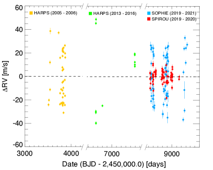
Figure 1: New SPIRou and SOPHIE RVs, together with the archival HARPS data used in this work.

3 Observations and data reduction

3.1 HARPS

Gl 388 was observed from 2005 to 2016 with the HARPS high-precision velocimeter (Mayor et al., 2003; Pepe et al., 2004) installed on the 3.6 m telescope at La Silla Observatory in Chile. The HARPS data set consists of 51 measurements, of which 39 were acquired between 2005 and 2006 (HARPS1 data set) and previously reported in Bonfils et al. (2013) and 12 are new measurements obtained between 2013 and 2016 (HARPS2 data set). Each spectrum covers the 380-690 nm spectral range with 71 orders at a median resolving power of 115000. Spectra were wavelength calibrated to a high accuracy using a simultaneous ThAr hollow cathode or Fabry-Pérot calibration lamp. Science-ready optical spectra were obtained from the ESO-archive facility and we measured RVs using the template-matching algorithm described in Astudillo-Defru et al. (2015). The summary of the HARPS1 and HARPS2 RV measurements is given in the Appendix. The median per visit precision of these RVs is 1.3 m s^-1, with a minimum of 1.2 and a maximum of 2.7 m s^-1.

3.2 SOPHIE

We obtained 71 RV measurements of Gl 388 between March 2, 2019 and April 23, 2021, with the SOPHIE high-resolution optical spectrograph (Perruchot et al., 2008; Bouchy et al., 2013) installed on the 1.93m Telescope of the Observatoire de Haute Provence (OHP) in southern France. The observations used the high-resolution mode ($R\sim$75000) and a simultaneous Fabry-Pèrot calibration lamp. SOPHIE covers a wavelength domain from 3872 to 6943 Å  across 38 spectral orders. Data were reduced with the SOPHIE data-reduction system (Bouchy et al., 2009; Heidari, 2022). RVs and their error bars were computed using a CCF technique with an empirical M5 mask, with a RV zero-point nightly correction based on measurements of RV standards (Boisse et al., 2010; Heidari et al., 2022). The summary of the SOPHIE RVs is given in the Appendix. The per visit precision of these RVs ranges from 2 to 7 m s^-1, with a median of 2.6 m s^-1.

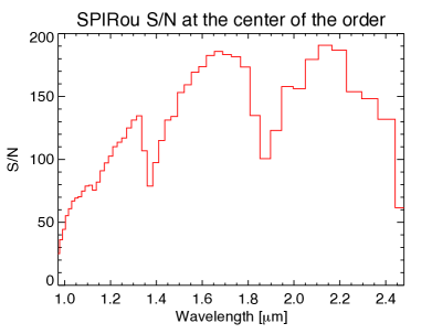
Figure 2: Example of the S/N per pixel at the center of the order achieved in the extracted 1D SPIRou spectrum of Gl 388.

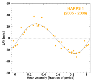
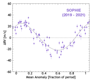
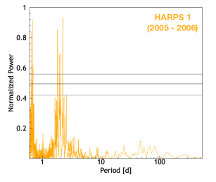
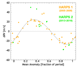
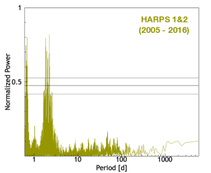
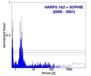
Figure 3: Periodograms and phase-folded RVs of the HARPS1, HARPS2, and SOPHIE data sets. The horizontal lines mark FAP levels of 0.1, 1, and 10%. A prominent peak is observed in all the periodograms at 2.23 days, the rotational period of the star, with aliases at 1.81 and 0.69 days. The DACE Keplerian model with period $P=$2.23 days used to phase-fold each data set is described in Table 17.

Table 2: HARPS and SOPHIE RV time series analysis.

	HARPS1	HARPS1+2	SOPHIE	HARPS1+2 & SOPHIE
	$(2005-2006)$	$(2005-2016)$	$(2019-2021)$	$(2005-2021)$
norm. power†	0.92	0.87	0.84	0.79
log10(FAP)${}_{\rm Analytical}^{\dagger}$	$<-15.95$	$<-12.4$	$<-15.95$	$<-15.95$
$P$ [days]	2.2270$\pm$0.0001	2.23099$\pm$0.00001	2.23001$\pm$0.0001	2.231023$\pm$0.000004
$K$ [m s-1 ]	25.6$\pm$0.3	25.9$\pm$0.3	23.6$\pm$0.5	24.6$\pm$0.2
ecc	0.08$\pm$0.01	0.08$\pm$0.01	0.08$\pm$0.02	0.03$\pm$0.01
$\omega$ [deg]	247$\pm$8	227$\pm$7	327$\pm$16	254$\pm$20
$M_{0}$ [deg]	242$\pm$17	138$\pm$7	151$\pm$28	101$\pm$20
O$-$C rms [ m s-1 ]	4.8	9.2	7.5	9.5

3.3 SPIRou

We observed Gl 388 on 74 epochs between February 14, 2019 and November 3, 2020, with SPIRou, the near-IR spectropolarimeter (Donati et al., 2020) installed on the 3.6 m Canada-France-Hawaii Telescope (CFHT) atop Mauna Kea (Hawaii). The SPIRou spectra cover from 0.96 to 2.50 $\mu$m at a resolving power of $R\sim 70000$. Figure 1 shows the time coverage of the HARPS, SOPHIE, and SPIRou observations. Each SPIRou visit obtains a Stokes V polarimetric sequence consisting in four 61s exposures with distinct positions of the Fresnel rhombs. The raw data were reduced using version v06132 of the SPIRou data reduction pipeline APERO (Cook et al., 2022), installed at the SPIRou Data Centre hosted at the Laboratoire d’Astrophysique de Marseille. Each 2D SPIRou spectrum consists of two science spectra, A and B, one per polarimetric channel, and one spectrum of a Fabry-Pérot étalon in the calibration channel C. Our RV analysis does not use the polarimetric information and uses combined extraction of the A and B science channels. The spectra were extracted, dark- and flat-field corrected, and wavelength calibrated using the nightly calibrations. Details of the wavelength calibration algorithm, which uses both a Uranium-Neon lamp and Fabry-Pérot exposures, is described in Hobson et al. (2021) and Cook et al. (2022). The 1D spectrum was then corrected for telluric absorption using a principal component analysis (PCA) method and a large library of spectra of telluric standard stars from nightly observations since 2018. The principle of the method is described in Artigau et al. (2014). Figure 2 displays the typical S/N per pixel achieved at the center of the order in one exposure. A S/N higher than 150 was achieved typically in the center of the H and K bands.

Measurements of RVs were extracted from the spectra with a line-by-line (LBL) algorithm described in Artigau et al. (2022). They were referred to the barycenter of the Solar System using the astropy routine barycorrpy, and corrected for the drift of the Fabry-Pérot and for changes in the RV zero point. The RV zero point correction was derived from observations of a set of RV standards that have been observed by SPIRou nightly since 2018. The final RV for a visit is the average of the RVs measured in each of the four spectra of the Stokes V sequence, and has a typical precision of 2 m s^-1. The summary of the SPIRou RVs is given in the Appendix.

Stokes $I$ and $V$ spectra were obtained from the same raw data employing the polarimetric reduction module of APERO. We then applied least-squares deconvolution (LSD; Donati et al. 1997; Kochukhov et al. 2010) to those spectra to extract average Stokes $I$ (polarized) and $V$ (circularly polarized) profiles. The line mask for LSD was generated via the Vienna Atomic Line Database (VALD, Gustafsson et al., 2008) from a synthetic spectrum with $T_{\mathrm{eff}}=3500$ K, $\log g=$ 5.0 cm s^-2, and $v_{\mathrm{micro}}=$ 1 km s^-1, and it contains 1400 atomic lines between 950 and 2600 nm deeper than 3% of the continuum level and with a known Landé factor (g_eff, i.e., the Zeeman effect sensitivity). The longitudinal magnetic field was computed from the average Stokes profiles using

$$B_{\ell}\;[G]=\frac{-2.14\cdot 10^{11}}{\lambda_{0}\mathrm{g}_{\mathrm{eff}}c}\frac{\int vV(v)dv}{\int(I_{c}-I)dv}\,,$$ (1)

where $\lambda_{0}$ and $\mathrm{g}_{\mathrm{eff}}$ are the normalization wavelength and the average Landé factor of the Stokes profiles, $c$ is the speed of light in vacuum, $v$ is the point-wise RV of the profile in the star’s rest frame, and $I_{c}$ is the continuum level (Donati et al., 1997). The integral in Eq. 1 was computed within $\pm$ 50 km s^-1 of the profile center to encompass the full line width in both Stokes $I$ and $V$. We exclude six February 2019 observations from the magnetic analysis presented here because an optical component of the instrument was malfunctioning at very low temperatures and affected those six circular polarization spectra. The summary of the SPIRou $B_{\ell}$ measurements is given in the Appendix.

4 Radial velocity analysis

4.1 HARPS and SOPHIE optical radial velocities

Using the DACE online interface hosted by the University of Geneva,    we  calculated  least-square  periodograms  for   the
HARPS1, HARPS2, and SOPHIE time series, both individually and combined. Figure 3 summarizes the periodograms obtained. All optical data sets produced a prominent peak at 2.23 days with analytical false alarm probabilities (FAP) well below 0.01% (see Table 17). We used DACE to fit a Keplerian model to each data set, using the 2.23 day peak to set the initial conditions. Table 17 summarizes the properties of these Keplerian fits and Figure 3 displays the corresponding phase-folded RVs. Even though the 2013$-$2016 HARPS2 data set has a larger dispersion than the 2005$-$2006 HARPS1 data set (see Figure 1), the combined HARPS1 + HARPS2 data set can be described by a similar period and semiamplitude to that of HARPS1, with the main difference being, $\omega$, the argument of periastron, and $M_{0}$, the mean anomaly at the reference time $t=0$. The 2019$-$2021 SOPHIE RV signal is very similar to the earlier HARPS1+2 signal, with a 2.23 day period retrieved in both data sets, but with a 2.3$\pm$0.6 m s^-1 difference between the semiamplitude of the Keplerian fit. The different orbital solutions in Table 17 converge to periods that differ very slightly but beyond their error bars. This could be due to a subtle change in the effective rotation period because of the combination of differential stellar rotation with a change in the latitude of the main spot. However, the 2.227, 2.230, and 2.231 day periods are aliases of each other for samplings of $\sim$3300 and $\sim$5000 days, which correspond to the average interval between the HARPS1 and HARPS2 acquisition periods and between the HARPS1 and SOPHIE ones (Figure 1), respectively. We therefore tentatively interpret these period differences as aliasing effects.

As illustrated by Figure 3, a single global Keplerian solution can describe all HARPS and SOPHIE RVs. It does, however, have larger residuals than separate fits to the HARPS or SOPHIE data alone (Table 17), indicating that although the optical RV signal is globally stable from 2005 to 2021, small variations are nevertheless present. The amplitude and phase differences between the HARPS and SOPHIE data and the relative constant period suggest that the optical RV signal is dominated by rotational modulation of a slightly variable stellar activity. Because the SOPHIE and SPIRou data were obtained quasi-simultaneously, we use only the SOPHIE data in our comparison with the near-IR RVs.

4.2 SPIRou radial velocities

The summary of the SPIRou RV measurements is provided in the Appendix. Figure 5 shows the phase-folded SPIRou and SOPHIE RVs at $P$=2.23 days. We can clearly see that the near-IR RVs do not match the periodic signal observed in the optical data, and that they are much flatter. Figure 5 displays the periodogram of the SPIRou RV data. There are no peaks with significance above the FAP 1% level, and most notably, there is no signal whatsoever at $P$=2.23 days. The dispersion of the SPIRou time series is just 5 m s^-1 rms; it clearly excludes the periodic signal of 24 m s^-1 semiamplitude observed in the optical RVs and the 16.6 m s^-1 stable RV component suggested in Kossakowski et al. (2022).

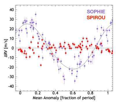
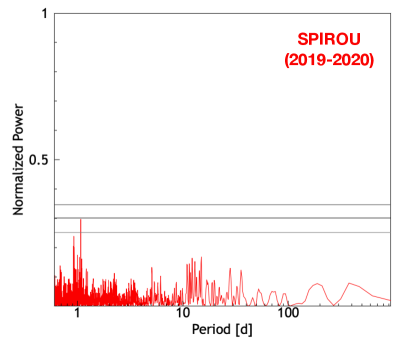
Figure 4: Phase-folded RV measurements of Gl 388 with SPIRou in the near-IR (red dots) and with SOPHIE (blue dots) in the optical. The gray line represents the Keplerian model with a period of 2.23 days and $K=$ 23.6 m s^-1 derived from the SOPHIE data (Table 17).

Figure 5: Periodogram of the SPIRou RV series. The horizontal lines mark FAP levels of 0.1, 1, and 10%. No peak is present at 2.23 days.

Previous RV observations with SPIRou show that a Keplerian signal of 20 m s^-1 is easily detected by the instrument. For example, in Moutou et al. (2020), SPIRou detected the $\sim$25 m s^-1 RV signal of the Rossiter-McLaughlin effect in the transiting extrasolar planet HD 189733b previously measured in the optical by HARPS (Triaud et al., 2009). SPIRou observations, using the LBL technique applied in this work, have detected planetary signals with amplitudes below 5 m s^-1, for example, in the star TOI-1759 (2.4 m s^-1, Martioli et al., 2022), and have shown flat RVs at a precision of 2.6 m s^-1 rms in Barnard’s star (Artigau et al., 2022), a star with the same spectral type as Gl 388.

The stability of the SPIRou measurements  in Gl 388 provides solid evidence rejecting the hypothesis that the RV modulation seen in the optical has a Doppler origin. We conclude that the periodic signal observed with HARPS and SOPHIE is mainly due to stellar activity, with a negligible contribution from any orbiting planet in a spin-orbit resonance.

4.3 Planet detection limits from the SPIRou radial velocities

We computed planet detection limits from the SPIRou RVs using Zechmeister & Kürster (2009) generalized Lomb-Scargle (GLS) periodograms as in Bonfils et al. (2013). The method obtains the upper limits by injecting signals in the time series at each period and determining the maximum amplitude that we can still miss with a given probability. We assume that the SPIRou time series contains no genuine planetary signal and for each period we inject a sinusoidal Keplerian signal at 12 equi-spaced phases. The amplitude (i.e., the planet signal strength) is then increased until the corresponding peak of the GLS periodogram reaches the 1% FAP level. We tested periods from 0.8 to 10000 days and derived the upper limit on the signal amplitude (and the corresponding projected mass) as a function of the period. The 1% FAP confidence level was computed from the levels of the highest peaks of 1000 permuted data sets, and the 1% upper limits’ function was obtained by sorting the power of peaks of all periodograms at each period.

For each period, the upper limit is the highest signal amplitude (at the worst phase) that could be present in the time series without creating a peak above the 1% FAP level. Figure 6 shows the projected mass as a function of the period at which 99% and 75% of the planets injected would be detected in the GLS periodogram of the SPIRou data. As described in Bonfils et al. (2013), the degraded upper limits for periods around one and two days are due to the data sampling and an unavoidable consequence of observing at night from a single location. Our analysis assumes circular orbits and uses the stellar parameters of Section 2. The SPIRou observations would have detected a 2.23 day period planet of 8 and 4 Earth-masses with 99% and 75% confidence levels, respectively.

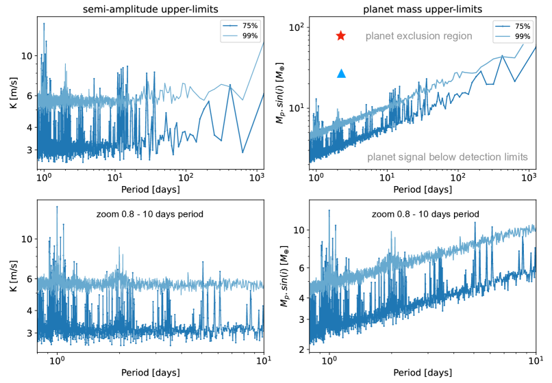
Figure 6: Detection limits in the SPIRou RV time series. Left panels: Upper limits in m s^-1 of the semiamplitude $K$ of the sinusoidal signal. Right panels: Upper limits in terms of the projected mass m sin(i). Objects with a projected mass above the limit are ruled out by the observed GLS periodogram with 99% (light blue) and 75% (dark blue) confidence levels (see text for details). Upper panels: Upper limits for periods from 0.8 to 1000 days. Lower panels: Zoom on the 0.8 to 10 day range. The red star indicates the location of the 0.24 M_J (76 M_⊕) planet in corotation claimed by Tuomi et al. (2018). The blue triangle shows the planet-mass equivalent (27 M_⊕) of the stable RV component in Kossakowski et al. (2022). Both are ruled out by the SPIRou data with a confidence higher than 99%.

4.4 Optical and near-IR radial velocity chromaticity effects.

Spots on the stellar surface can induce RV signals modulated by the stellar rotation. We have demonstrated that the Gl 388 RV signal is strongly chromatic between optical and near-IR wavelengths. In this section, we explore how the RV signals vary when the RV is measured selecting specific regions in the spectrum. Our objective is to explore whether there could be a chromatic dependence of the RV signal inside the optical or the near-IR domain.

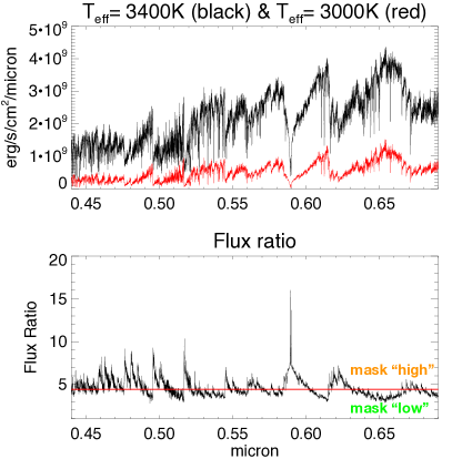
Figure 15: Regions in the optical spectra used to define the CCF masks to study the chromaticity of the SOPHIE RVs. Upper panel: Theoretical PHOENIX medium resolution models of stellar atmospheres with $T_{\rm eff}=3400$ and $3000$ K in the SOPHIE wavelength range. Lower panel: Flux ratio of the atmosphere models of the upper panel. The horizontal red line is the median flux ratio. Lines of the SOPHIE M-star mask in the regions over the median flux ratio constitute the high-contrast mask, and the lines located below the median constitute the low-contrast mask.

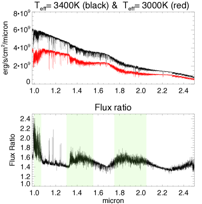
Figure 17: Regions in the near-IR spectra used to select the LBL lines to study the chromaticity of the SPIRou RVs. Upper panel: Theoretical PHOENIX medium resolution models of stellar atmospheres with $T_{\rm eff}=3400$ and $3000$ K in the SPIRou wavelength range. Lower panel: Flux ratio of the atmosphere models of the upper panel. The regions highlighted in light green are the high-contrast flux ratio regions used for filtering the LBL RV measurements.

In a first test, we computed the RV selecting the regions in the spectra based on the expected flux contrast between photospheric and spot model spectra. For this test, we used the ratio between PHOENIX (Husser et al., 2013) medium resolution synthetic stellar spectra with temperatures of 3400 K and 3000 K, representing the stellar photosphere and the spot (see Figures 15 and 17 in the Appendix). We selected a 400 K temperature difference between the photosphere and the spot as it is typical for a mid-M star (Berdyugina, 2005; Barnes et al., 2015). To analyze the SOPHIE data, we constructed two cross-correlation masks starting from the M-star mask used to compute the RVs: a ”high-contrast” mask, which contains the lines that fall in the regions where the flux ratio is higher than its median value, and a ”low-contrast” mask with the lines that fall in the complementary regions where the flux ratio is below its median value. The ”high” and ”low” contrast regions of SOPHIE are illustrated in Figure 15 in the Appendix. To analyze the SPIRou data, we defined the low and high contrast regions in an analogous manner as illustrated in Figure 17 in the Appendix. The LBL method calculates a RV for each ”line” in the spectrum and then computes a final RV as a weighted average of the lines’ RVs. We filtered the LBL file of each visit selecting the lines that fell to the low and high contrast regions, and then computed the final RV for the low and for the high case. The SPIRou RVs were corrected for the RV zero point as previously described.

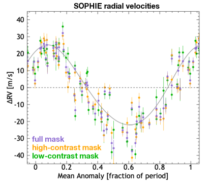
Figure 16: Phase-folded RVs measured with SOPHIE using the full, high-contrast, and low-contrast SOPHIE M-type star CCF masks. The model is the Keplerian model derived from SOPHIE’s full-mask RVs.

The properties of SOPHIE’s high, low, and ”full” RV time series and periodograms are given in Table 3. The three masks produce similar individual RV measurements uncertainties of about 3 m s^-1, with the high-contrast mask giving a slightly better precision of 2.8 m s^-1. The RV zero points of the low-contrast and high-contrast masks differ slightly from that of the full mask, $-12$ m s^-1 for the low-contrast mask and by +10 m s^-1 for the high-contrast mask. After correcting the three time series from their RV zero point, we found largely equivalent results for the three masks. All of them produce periodograms with a peak at the same 2.23 day period and have a similar phase for the signal. The amplitude, however, does differ by a small but significant 2.5 m s^-1 between the RVs calculated with the low and the high mask. Figure 16 in the Appendix displays the phase-folded SOPHIE RV time series obtained with the three masks, they differ a little.

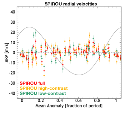
Figure 18: Phase-folded SPIRou RVs for the LBL calculation including the full, high-contrast, and low-contrast lines. The model is the Keplerian model for the SOPHIE full-mask data.

The properties of SPIRou’s high, low, and full RV time series are summarized in Table 4. The phase-folded RVs are given in Figure 18 in the Appendix. We find no significant differences between the SPIRou low, high and full RV time series: all three gave the same median RV point, and in terms of RV performances, the difference between the high and low time series is below 1 m s^-1. The best performance is obtained when the full wavelength range is taken into account ($5$ m s^-1 rms).

Table 3: SOPHIE RV time series properties obtained with the full, low-contrast, and high-contrast masks.

	full	high	low
median RV [km s-1]	12.505	12.515	12.493
mean $\sigma_{\rm RV}$ [m s-1]	3.0	2.8	3.2
norm. power †	0.84	0.81	0.75
log10(FAP)Analytical†	$<-15.95$	$<-15.95$	$<-15.95$
$P$ [days]	2.2300$\pm$0.0001	2.2301$\pm$0.0001	2.2300$\pm$0.0001
$K$ [m s-1]	23.6$\pm$0.5	24.7$\pm$0.5	22.4$\pm$0.5
ecc	0.08$\pm$0.02	0.04$\pm$0.02	0.16$\pm$0.02
$\omega$ [deg]	327$\pm$16	317$\pm$28	340$\pm$8
$L_{0}$	120$\pm$21	133$\pm$21	105$\pm$20
O$-$C rms [m s-1]	7.5	8.4	8.0

Table 4: SPIRou RV time series properties for the high, low, and full regions, and the Y, H, J, and K bands.

Band	median RV	rms
	[km s-1]	[m s-1]
high	12.696	6.7
low	12.696	5.9
full	12.696	5.0
Y	12.695	37.4
J	12.695	22.2
H	12.696	6.2
K	12.696	9.2

Table 5: Confidence interval (1$\sigma$) on the semiamplitude $K$ of a sinusoidal fit, with a fixed period (2.23 days) and phase, to the RV time series per photometry band.

Band	$K$ sin. fit
	[m s-1]
B (SOPHIE)	$24.9_{-3.1}^{+3.1}$
V (SOPHIE)	$23.0_{-3.4}^{+3.4}$
R (SOPHIE)	$23.0_{-3.7}^{+3.7}$
full BVR	$22.7_{-3.4}^{+3.4}$
Y (SPIRou)	$17.1_{-20}^{+20}$
J (SPIRou)	$6.3_{-14.4}^{+14.4}$
H (SPIRou)	$-1.2_{-3.9}^{+3.9}$
K (SPIRou)	$-4.9_{-5.5}^{+5.5}$
full YJHK	$-2.1_{-2.8}^{+2.8}$

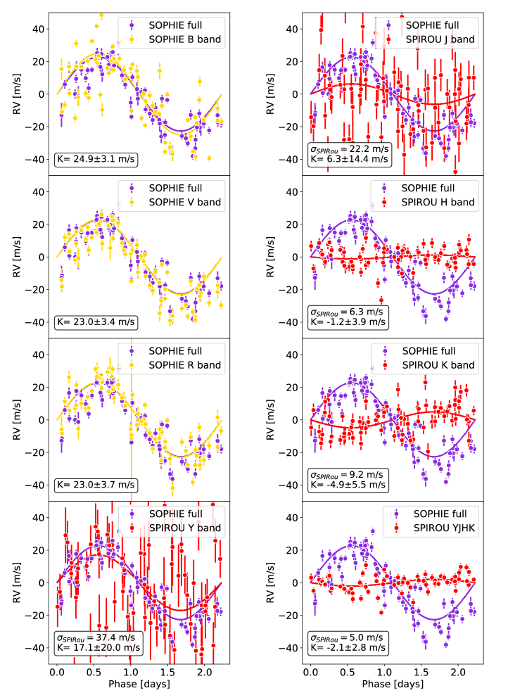
Figure 19: Phase-folded RVs in the B, V, and R bands for SOPHIE (yellow points) and in the Y, J, H, and K bands for SPIRou (red points). The best sinusoidal fit per band is given in a continuous line following the same color convention. For comparison, in each panel, we include (blue color) the phase-folded RVs and sinusoidal fit obtained in the full SOPHIE range. For the sinusoidal fit and RV phase-folding, the phase (i.e., T₀ ) and period (2.23 days) are the same for all the time series. It is important to note that although a sinusoidal fit is possible in the SPIRou data, the periodograms show that there is no signal at the 2.23 day period (see Figure 20). The SPIRou data are compatible with a straight line with $K=0$ m s^-1. The sinusoidal fit to the SPIRou data enabled us to set an upper limit on the RV dispersion that is smaller than the rms value.

In a second test for RV chromaticity, we examined the RV time series obtained per photometry band. In the case of the SOPHIE observations, we calculated the RVs using the same M dwarf mask, but this time we selected the orders used to build the CCF. For the B band, we selected the orders 3 to 18 ($4008.5-4962.7$ Å), for the V band the orders 19 to 31 ($4934.9-6092$ Å), and for the R band the orders 32 to 38 ($6077-6943$ Å). For SPIRou, we analyzed the RV time series obtained by applying the LBL algorithm to individual near-IR bands within the SPIRou spectral domain: Y ($900.0-1113.40$ nm), J ($1153.59-1354.42$ nm), H ($1462.89-1808.54$ nm), and K ($1957.79-2343.10$ nm) bands. Table 4 displays the median and rms of the RV time series for each SPIRou band. Figure 19 in the Appendix shows the SOPHIE and SPIRou RV time series per band phase-folded using a period of 2.23 days. In all data sets, we used the same T₀ such that the SOPHIE RVs have phase = 0 at $v=0$ m s^-1. In each RV time series, we fit a sinusoidal signal with a fixed period of 2.23 days and a phase = 0. Table 5 shows the retrieved best-fit semiamplitude $K$ in m s^-1 with a $1\sigma$ error bar.

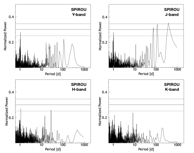
Figure 20: Periodograms of the SPIRou RVs in the Y, J, H, and K bands. The horizontal lines mark the FAP levels of 0.1, 1, and 10%. No periodic signal is observed in any of the bands at 2.23 days.

In the case of the SOPHIE data, the B, V, and R RV time series display, within 1$\sigma$, the same sinusoidal signal with a very similar amplitude. A slight decrease of $-2$ m s^-1 in the semiamplitude with respect to the B band is seen in the V and R bands; however, the difference is smaller than the $3-4$ m s^-1 $1\sigma$ uncertainty in the semiamplitude. In the SPIRou data, the RV uncertainty per visit and the RV dispersion differs from band to band, as expected from their respective RV information content (Artigau et al., 2018). The Y and J bands display the highest RV dispersion (37 and 22 m s^-1 rms, respectively), followed by the K band with 9.2 m s^-1 rms, and the H band performs best with 6.2 m s^-1 rms. The best overall performance is obtained using the full spectral domain (5.0 m s^-1 rms). The sinusoidal fits in the Y and J band hint at a periodic signal similar to that observed in the optical but with a weaker amplitude. However, when the periodogram analysis is performed (see Figure  20 in the Appendix), none of the near-IR RV time series per band display a significant peak at $P$=2.23 days. The semiamplitudes’ error shows that $K$ is compatible with 0 m s^-1 within the 1$\sigma$ uncertainty. The sinusoidal model is in fact fitting the noise dispersion. The sinusoidal fit enables, nevertheless, the upper limit of the semiamplitude to be lowered to 17, 6, 1, 5, and 2 m s^-1 for the Y, J, H, K, and the full near-IR SPIRou domain, respectively (see Table 5). The difference in semiamplitude between the H and K bands could suggest a difference in RV dispersion due to the onset of magnetic effects (i.e., the Zeeman broadening), but the difference can also be due to a difference in the intrinsic performances between the K and the H band due to the telluric absorption and the S/N of the spectra. The increase in RV semiamplitude at $\lambda>1500$ nm of tens of m s^-1 predicted by some theoretical models (see for example Fig. 5 in Kossakowski et al. (2022)) is not observed in our SPIRou’s Gl 388 data.

In summary, we detect a strong chromatic effect in the RV between the optical and near-IR wavelengths taken as a whole; however, we do not observe strong chromatic effects within the individual photometry bands. A small but significant difference is found in the RV analysis between high and low CCF masks of SOPHIE. No difference has been found in other tests.

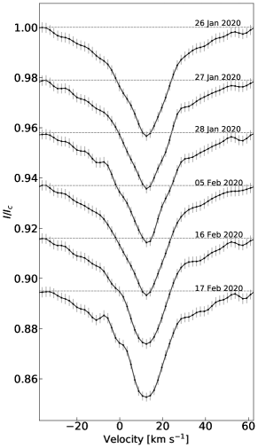
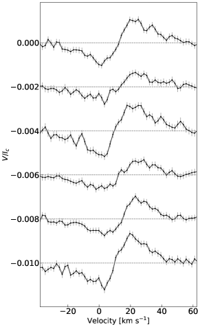
Figure 7: Six representative continuum normalized Stokes $I$ (left) and $V$ (right) profiles from SPIRou observations collected in early 2020. The profiles are vertically shifted for visualization purposes.

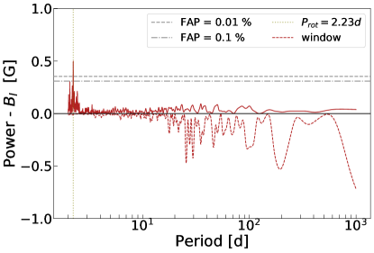
Figure 8: Generalized Lomb-Scargle periodogram and window function of the SPIRou $B_{\ell}$ time series. A long-term variation of the $B_{\ell}$ data set was filtered out beforehand to prevent it from perturbing the period analysis. The highly significant peak (FAP$<$ 0.01%) at 2.23$\pm$0.01 days matches the rotation period reported in the literature and the period observed in the SOPHIE RV data.

5 Activity analysis

5.1 SPIRou longitudinal magnetic field measurements

Figure 7 presents examples of the measured SPIRou Stokes $I$ and Stokes $V$ profiles, which a future publication (Bellotti et al. in prep) will use for a full ZDI analysis. Table LABEL:SPIRouRVBlTable summarizes the $B_{\ell}$ measurements obtained from those profiles. We note that $B_{\ell}$ is detected at every epoch and varies from $-55$ G to $-277$ G, with a median of $-194$ G, and a median noise of 15 G. Figure 8 displays the GLS periodogram of the $B_{\ell}$ time series. Although stellar activity signals sometimes lose coherency over long time spans, the periodogram here shows a single, clear, narrow, and highly significant (FAP$<$ 0.01%) peak at 2.23$\pm$0.01 days. This period is consistent with those derived from both the optical spectropolarimetric observations of Morin et al. (2008) and the SOPHIE, HARPS, HARPS-N, and HIRES RV measurements. The periodogram structure at longer periods is likely due to aliases of the observation window. Previous studies have shown that $B_{\ell}$ is a reliable magnetic activity tracer (Folsom et al., 2016; Hébrard et al., 2016a) and that it varies on the stellar rotation period. The peak in the $B_{\ell}$ periodogram is thus further evidence that the rotational period of Gl 388 is 2.23 days and that the RV signal in the optical is due to stellar activity. Thus, while the stellar rotation signal of Gl 388 is not detected in the SPIRou RV data, it is clearly detected in the $B_{\ell}$ time series.

Table 6: Prior and posterior distributions of the quasi-periodic GP model of the SPIRou $B_{\ell}$ measurements and the HARPS and SOPHIE RV time series.

Parameter	Prior distribution		Posterior distribution
			ln units	linear units
GP SPIRou $B_{\ell}$
Amplitude [G]	$\ln{A}$	$\mathcal{U}\left(2,6\right)$	$4.38^{+0.45}_{-0.34}$	$80^{+45}_{-23}$
Decay time [days]	$\ln{l}$	$\mathcal{U}\left(2,8\right)$	$5.37^{+0.32}_{-0.29}$	$216^{+82}_{-54}$
Smoothing parameter	$\ln{\Gamma}$	$\mathcal{U}\left(-5,3\right)$	$-1.47^{+0.71}_{-0.85}$	$0.23^{+0.24}_{-0.13}$
Cycle length (period)  [days]	$\ln{P}$	$\mathcal{U}\left(\ln{\left(2.20\right)},\ln{\left(2.25\right)}\right)$	$0.80221^{+0.00070}_{-0.00058}$	$2.2305^{+0.0016}_{-0.0013}$
Uncorr. Noise [G]	$\ln{\sigma}$	$\mathcal{U}\left(-30,15\right)$	$-3.7^{+4.1}_{-4.3}$	$0.03^{+1.52}_{-0.02}$
GP HARPS & SOPHIE optical RVs
Offset [km s-1]	$V_{0}$	median(RV) + $\mathcal{U}\left(-10,10\right)$		$0.00^{+0.01}_{-0.01}$
Amplitude [km s-1]	$\ln{A}$	$\mathcal{U}\left(-5,5\right)$	$-3.30^{+0.24}_{-0.22}$	$0.037^{+0.010}_{-0.007}$
Decay time [days]	$\ln{l}$	$B_{\ell}$ Posterior	$5.32^{+0.16}_{-0.17}$	$205^{+36}_{-32}$
Smoothing parameter	$\ln{\Gamma}$	$B_{\ell}$ Posterior	$-0.69^{+0.40}_{-0.40}$	$0.50^{+0.26}_{-0.17}$
Cycle length (period) [days]	$\ln{P}$	$B_{\ell}$ Posterior	$0.80146^{+0.00037}_{-0.00041}$	$2.2288^{+0.0008}_{-0.0009}$
Uncorr. Noise [km s-1]	$\ln{\sigma}$	$\mathcal{U}\left(-10,5\right)$	$-5.61^{+0.13}_{-0.13}$	$0.0037^{+0.0005}_{-0.0004}$

5.2 Gaussian process analysis of the optical HARPS and SOPHIE data using SPIRou’s $B_{\ell}$ as an activity proxy.

5.2.1 Gaussian process modeling with a variable decay time.

Gaussian process (GP) modeling of RV time series is nowadays a standard procedure to correct for the stellar activity RV jitter and to search for Keplerian signals (e.g., Rajpaul et al., 2015; Suárez Mascareño et al., 2020; Klein et al., 2021; Kossakowski et al., 2022). The measurements of the $B_{\ell}$ obtained with SPIRou are quasi-simultaneous with the RV measurements obtained with SOPHIE; $B_{\ell}$ therefore provides an excellent proxy of stellar activity for modeling the optical RVs within the GP framework. The use of $B_{\ell}$ as a stellar activity indicator is motivated by the close physical link between stellar magnetic activity and the presence of spots and plages, and the results of spectropolarimetry ZDI studies in M dwarfs (e.g., Hébrard et al., 2014, 2016b), which have shown that the determination of the stellar magnetic topology enable us to filter the RV activity jitter in stars with moderate rotation.

We modeled the combined HARPS and SOPHIE RVs running two sequential quasi-periodic Gaussian processes (QP GP). We first ran a GP on the SPIRou $B_{\ell}$ time series. Then, using the decay time, smoothing, and cycle length (i.e., rotation period) posterior distributions of the $B_{\ell}$ GP as priors, we ran a second GP on the optical RV series. For the $B_{\ell}$ GP, we used uniform distributions for the priors of the amplitude, decay time, smoothing, cycle length, and uncorrelated noise (see further details in Table 6). This modeling strategy has the underlying assumption that the RV effects and the magnetic field have the same temporal behavior. Our principal aim is to check how well the optical RVs could be described by a QP GP model in which the stable component is associated with rotation and the variable component is associated with changes in magnetic activity, and to determine the typical timescale of that variable component.

For our analysis we used the GP package george (Foreman-Mackey, 2015) which uses a quasi-periodic kernel of the form

$$k\left(\Delta t\right)=A\exp{\left(-\frac{\Delta t^{2}}{2l^{2}}\right)}\exp{\left(-\Gamma\sin^{2}{\left(\frac{\pi}{P}\Delta t\right)}\right)}+\sigma^{2}\delta\left(\Delta t\right),$$ (2)

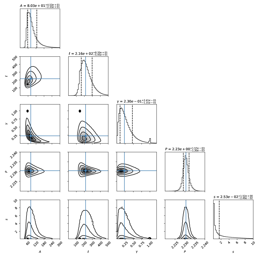
Figure 21: Corner plot of the quasi-periodic GP fit of the SPIRou longitudinal magnetic field (B_ℓ) time series. The description of the meaning of the variables is given in Table 6.

where $A$ is the amplitude, $\Gamma$ is the smoothing parameter, $l$ is the decay time in days, $P$ is the period (i.e., the cycle length) in days, and $\sigma$ is the uncorrelated noise (s in the corner plots). We sampled the distribution of the hyperparameters using a Markov chain Monte Carlo (MCMC) framework using the EMCEE tool (Foreman-Mackey et al., 2013) with 100000 samples and 10000 burn-in samples. Figure 9 and Table 6 summarize the results of the GP modeling of the $B_{\ell}$ time series. The corner plots are in Figure 21 in the Appendix. The main result of the $B_{\ell}$ GP is an improved determination of the stellar rotational period to $2.2305^{+0.0016}_{-0.0013}$ days. It is a similar value to that retrieved using the $B_{\ell}$ periodogram analysis, however, it has a smaller uncertainty. The decay time obtained in the $B_{\ell}$ time series is $216^{+82}_{-54}$ days.

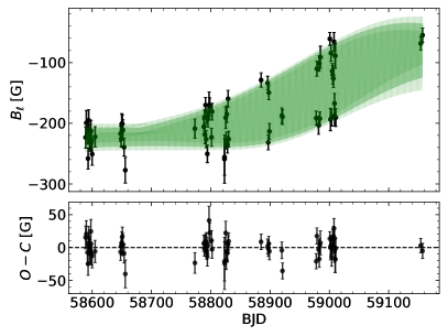
Figure 9: Longitudinal magnetic field ($B_{\ell}$) time series (black dots) and its QP GP model fit (green-line). Details of the GP are given in Table 6. The corner plot of the fit is given in Figure 21 in the Appendix.

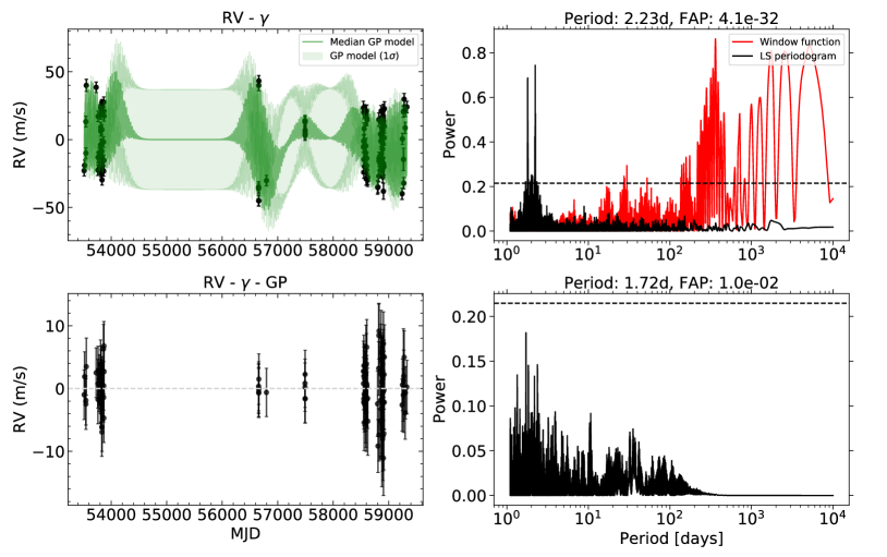
Figure 10: Summary of the GP analysis of the optical RV time series using SPIRou’s $B_{\ell}$ as an activity proxy. Upper left: QP GP fit (green line) to the HARPS and SOPHIE optical RV time series (black points). The median value of the raw RV is denoted by $\gamma$. Upper right: Periodogram of the RV data and window function before the QP GP fit. The horizontal line is the FAP=0.1%. Lower left: Residuals in the optical RVs after the subtraction of the QP GP fit. Lower right: Periodogram of the RV residuals after subtraction of the QP GP fit. In the top of each periodogram, the period, and FAP of the strongest peak are given. Details of the GP model are summarized in Table 6. The corner plot of the fit is given in Figure 22 in the Appendix.

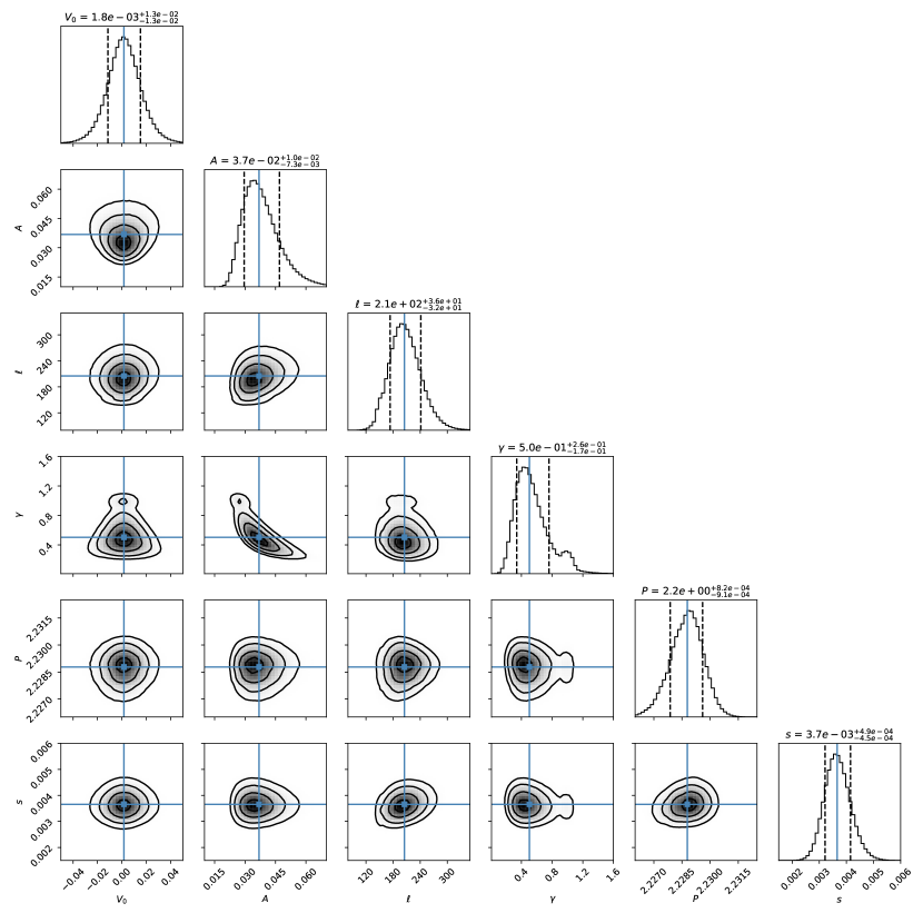
Figure 22: Corner plot of the quasi-periodic GP fit of HARPS and SOPHIE RV time series. The description of the meaning of the variables is given in Table 6.

The results of the GP model of the optical RVs are given in Figure 10 and in Table 6. The GP corner plots are provided in Figure 22 in the Appendix. We obtained in the GP of the RVs a period of $2.2288^{+0.0008}_{-0.0009}$ days, which is a similar value within the error bars to that obtained in the $B_{\ell}$ GP. The decay time obtained in the RV GP is $205^{+36}_{-32}$ days, a value that is also consistent within the error bars with the decay time obtained in the $B_{\ell}$ GP. The decay time of $\sim$200 days of the RV is shorter than the interval of time that separates the HARPS1, HARPS2, and SOPHIE observing campaigns. Therefore, each campaign can be considered as independent with respect to the variable component of the activity in the RV jitter. The similarity of the period and the decay time of the $B_{\ell}$ GP and RV GP suggests that the RV jitter is related to changes in the magnetic activity, but it can also be due to the very fact the $B_{\ell}$ GP has been used to set the priors of the RV GP model. The bottom panels of Figure 10 display the residuals of the optical RV time series and their periodogram after subtraction of the RV GP model. After GP correction, the rms of the time series is 3.7 m s^-1 and there is no evidence for periodic signals.

The main conclusion from our GP modeling is that the RV model anchored in the $B_{\ell}$ as an activity proxy provides a good description of the observed optical RV time series variability. This suggests that the rotationally modulated activity jitter observed in the optical is indeed probably linked to magnetic activity.

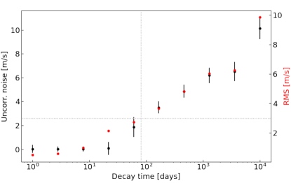
Figure 11: Uncorrelated noise and RV rms as a function of the decay time in the QP GP model of the optical HARPS and SOPHIE RV time series. The horizontal line in gray dots shows the typical accuracy of SOPHIE RVs (3 m s^-1). The vertical line in gray dots indicates the decay time of 80 days.

5.2.2 Gaussian process modeling with a fixed decay time.

In the previous analysis, we have enabled the decay time to be variable in the GP. The consequence of this assumption is that for short decay times, the GP by construction does not keep the phase constant between the various sets of optical RV data. This analysis leaves the question unanswered of whether is it still possible to fit all the optical RV data with a slowly evolving pattern that does not lose phase from run to run (i.e., whether the RV time series can be described with a GP with a long decay time), in addition to the question of how long the decay time can be before the uncorrelated noise and the RV rms start to increase. To explore the influence of the decay time in the uncorrelated noise and the RV rms, and to test whether a very long decay time ($>$1000 days) could describe the data, we ran a series of QP GPs on the optical RV data sets, by fixing in each the decay time to different values from 1 to 10,000 days. Our results are summarized in Figure 11 where we show the evolution of the uncorrelated noise and the RV rms as a function of the decay time. We observe that as soon the decay time becomes larger than 10 days, the uncorrelated noise and the RV rms increase. We recall, however, that the mean RV error in the SOPHIE RVs is $\sim$2.6 m s^-1; therefore, models displaying a lower RV rms are, in fact, fitting the noise. Figure 11 indicates that the RV rms becomes higher than 3 m s^-1 rms for decay times larger than 80 days. The decay time on the order of hundreds of days suggested both by the variable and fixed decay time GP modeling indicates that the RV jitter is evolving with time on a timescale of less than a year, conversely to what Tuomi et al. (2018) claim.

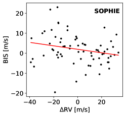
Figure 12: BIS versus RV for the SOPHIE data. The red line indicates the linear fit between these variables. The Pearson’s coefficient is $-$0.23, which indicates a weak anticorrelation.

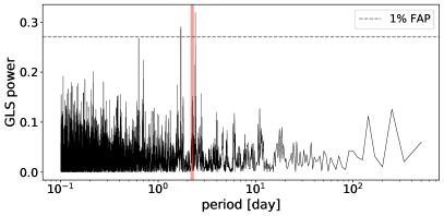
Figure 13: Generalized Lomb-Scargle periodogram of the SOPHIE bisector time series. The gray dashed line marks the 1% FAP. The highest peak in the periodogram corresponds to a 2.4 day period. The red vertical line indicates the location of the 2.23 day period.

5.3 Line shape analysis

Stellar activity changes the spectral line profiles, which in turn induces RV variations. The bisector inverse slope (BIS) is a line shape metric defined as the difference between the velocity at the top and the bottom of the cross-correlation function (Queloz et al., 2001). Figure 12 plots the BIS of the cross-correlation function against the RV for the SOPHIE data set. The two quantities are slightly anticorrelated with a Pearson coefficient $R$ of $-$0.23 (p-value = 0.05). This anticorrelation is weaker than the $R$ of $-$0.81 obtained by Bonfils et al. (2013) with HARPS. This difference may be due to the higher spectral resolution of HARPS (R=120 000) in comparison with SOPHIE (R=70 000) since the BIS strongly depends on this spectrograph feature (Desort et al., 2007). Figure 13 shows the GLS periodogram of the SOPHIE bisector time series, with a highest peak at 2.4 days.

Within the LBL framework which we used for the SPIRou spectra, we adopted the second and third derivatives of the LBL line profiles as line-shape diagnostics (Artigau et al., 2022, Cortez-Zuleta, in prep.). The second derivative can be interpreted as a proxy for the full-width half-maximum (FWHM) of the CCF, and the third derivative as a proxy for its BIS. The GLS periodograms of the time series of these second and third derivatives show no peak with a FAP below 1% (see Figure 14).

5.4 Activity indicators

The S index and the $\rm H\alpha$ index are widely used tracers of stellar chromospheric activity in the optical domain. They were measured from the SOPHIE spectra following the methods of Boisse et al. (2009) and Boisse et al. (2010), respectively. We computed GLS periodograms for both indices (Figure 14) and searched for periodic signals. None of the peaks in either periodogram rise to the 1% FAP line. We note that one of the highest peaks of the $\rm H\alpha$ periodogram is located at 4.2 days, which is close to the $\rm 2\times P$ subharmonic of the 2.23 day rotation period, but this might be coincidental.

Activity indicators are not as well established in the near-IR domain. We analyzed the temporal evolution of time series of the pseudo-equivalent width (pEW) of four atomic lines that were previously tested in the optical domain and/or for Sun-like stars: Aluminum I ($\lambda$ 13154 Å) (Spina et al., 2020), Potassium I ($\lambda$ 12435 Å) (Barrado y Navascués et al., 2001; Robertson et al., 2016; Terrien et al., 2022), Iron I ($\lambda$ 11693 Å) (Yana Galarza et al., 2019; Cretignier et al., 2020), and Titanium I ($\lambda$ 10499 Å) (Spina et al., 2020). The details of the method will be described in Cortes-Zuleta et al. (in prep).

Figure 14 displays the GLS periodogram of the pEW of these four near-IR lines. There is no high significant periodicity for the periodograms of Iron, Potassium, and Titanium that are not related to the spectral window function. The Aluminum periodogram is the only one where peaks rise above the 1% FAP line. These peaks are concentrated around the  1 day peak due to the sampling and produce the observed the long-period (¿10 days) aliases.

Due to the low inclination of Gl 388, one pole is within $\sim$20 degrees of the observer’s line of sight. This strongly reduces the modulation of activity indicators by stellar rotation. Activity features, such as spots, close to the observed pole will be in view for their full lifetime; thus, their pEW and projected velocity change little with rotation. Most of the stellar activity indicators tested in this work indeed do not vary on the 2.23 day stellar rotation period, which is unambiguously determined by the analysis of the longitudinal magnetic field (Section 5.1). The lack of variability on the stellar rotation period is therefore expected, particularly for the near-IR SPIRou data which have much lower RV jitter from activity than SOPHIE or HARPS in the optical (e.g., this work and Reiners et al., 2010). Besides SPIRou $B_{\ell}$ which is, in fact, an activity indicator modulated with the stellar rotation, the SOPHIE BIS is the only activity indicator in the spectra to be found to vary on a period (2.4 days) close to the stellar rotation period. The SOPHIE BIS exhibits a periodic variation with the stellar rotation because the BIS is sensitive to small changes in the line profile symmetry.

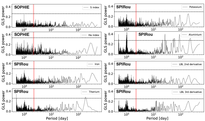
Figure 14: Generalized Lomb-Scargle periodograms of the activity indicators measured in the SOPHIE and SPIRou spectra. The dashed line marks the 1% FAP. The vertical red line indicates the 2.23 day period.

6 Conclusions

Radial velocity searches for planets around nearby M dwarfs are our best chance to identify rocky planets in the habitable zone that can be characterized by future instruments (e.g., Doyon et al., 2014; Beichman et al., 2014; Snellen et al., 2015; Lovis et al., 2017). M dwarfs have great potential as targets because the expected RV signature of an Earth-like planet in the habitable zone is within the sensitivity limits of current ground-based high-resolution velocimeters. However, many nearby M dwarfs are magnetically active. The spots and plages in their atmospheres present a challenge to RV planet searches since they can induce RV signatures that mimic those of a planet.

In this paper, we have presented contemporaneous new RV and spectropolarimetry observations of the magnetically active M dwarf Gl 388 obtained between 2019 and 2021, with the optical high-resolution spectrometer SOPHIE at OHP and the near-IR high-resolution spectropolarimeter SPIRou at CHFT. Our observations were obtained ten to fifteen years after previous RV measurements with HARPS at la Silla (2005 and 2006) and optical spectropolarimetry observations with ESPaDOnS at CFHT (2007 and 2008).

The new SOPHIE RVs vary on a 2.23$\pm$0.01 day period with 23.6$\pm$0.5 m s^-1 amplitude, which is consistent with the earlier HARPS observations. The two optical data sets can be jointly fit with a single Keplerian solution, which however has larger residuals than separate fits to the individual data sets. This can be explained by a subtle amplitude or phase change between the HARPS and SOPHIE epochs due to interactions between stellar differential rotation and changes in the average latitude of the spots. The HARPS data alone have long provided strong evidence that the optical RV signal is due to stellar activity (Bonfils et al., 2013; Reiners et al., 2013). The new SPIRou data display no periodic signal and their 5 m s^-1 dispersion is well below the 23.6$\pm$0.5 amplitude of the optical RV signal, removing any possible doubt that the latter is indeed due to activity, and it cannot be from the Doppler effect. The HARPS and SOPHIE data demonstrate that activity can induce a RV signal that is largely stable well over a decade, even in a star as active as Gl 388. The long-term stability of the Gl 388 RV signal shows how easily an activity signature in optical RV measurements can be misinterpreted as evidence for a planet (e.g., Tuomi et al., 2018).

The SPIRou campaign on Gl 388 spectacularly demonstrates the lower sensitivity of the near-IR RVs (at least those obtained by an LBL method) to stellar magnetic activity. This opens the way to perform exoplanet searches around stars which so far have been hardly studied or excluded from studies in the optical because of their activity. This also indicates that in some cases, when it is difficult to separate an RV activity effect from a Keplerian one, the use of near-IR RVs in addition to optical RVs is a crucial tool to remove spurious signals. For Gl 205, a star quieter than AD Leo, Cortes-Zuleta et al. (2023) demonstrate that the RV jitter can also be present in the IR but at a different phase or with a different shape than in the optical, possibly allowing filtering. The use of the near-IR RVs is of high relevance for the search of Earth-like planets in the habitable zone around M dwarfs (e.g., Artigau et al., 2022). With lower planetary masses, the combination of data from several instruments, and the need for activity filtering, a growing number of spurious signals is possible. To use near-IR RVs in addition to optical RVs it is important to consolidate optical RV surveys with long-term follow-up campaigns.

Our SPIRou observations additionally reiterate how effective spectropolarimetry is at determining the stellar rotation period from the variations of the longitudinal magnetic field. We measured a rotation period of 2.2305$\pm$0.0016 days from the SPIRou $B_{\ell}$ time series. ESPaDOnS and SPIRou, using the same technique at different wavelengths, produce essentially identical measurements of the stellar rotation period. Spectropolarimetry can determine the rotation period independently of photometry, which is particularly relevant for stars with a complex photometric time series behavior, and it can independently measure the rotation period and the inclination.

Appendix A SOPHIE and SPIRou chromaticity

Appendix B Corner plots of the quasi-periodic Gaussian process analysis.

Appendix C Radial velocity measurements

Table 7: HARPS RV measurements of Gl 388

DATE	BJD $-$ 2400000	$\delta$ RV	$\sigma_{\delta{\rm RV}}$
[yyyy-mm-dd]	[days]	[m/s]	[m/s]
2005-05-21	53511.54684	-21.1	1.5
2005-05-30	53520.52047	-17.2	1.5
2005-06-21	53543.48083	15.0	1.7
2005-06-22	53544.45178	-8.2	1.4
2005-06-28	53550.45964	41.7	2.7
2005-12-24	53728.86477	40.3	1.5
2006-01-23	53758.75397	-20.7	1.3
2006-01-25	53760.75468	-11.3	1.3
2006-01-26	53761.78002	18.9	1.3
2006-02-17	53783.72555	-7.9	1.3
2006-02-19	53785.72637	-19.8	1.3
2006-03-15	53809.65993	-2.1	1.2
2006-03-16	53810.67672	10.7	1.2
2006-03-17	53811.67496	8.2	1.2
2006-03-18	53812.66370	-8.8	1.5
2006-03-19	53813.65843	20.4	1.2
2006-03-20	53814.65398	-20.7	1.4
2006-03-21	53815.57020	25.5	1.3
2006-03-21	53815.62108	25.6	1.2
2006-03-21	53815.73541	24.9	1.2
2006-03-22	53816.54328	-14.8	1.3
2006-03-22	53816.65524	-19.2	1.2
2006-03-22	53816.72113	-21.8	1.3
2006-03-23	53817.54998	24.3	1.2
2006-03-23	53817.67492	26.8	1.3
2006-04-04	53829.61461	-1.2	1.2
2006-04-05	53830.53967	-6.7	1.3
2006-04-06	53831.66939	9.1	1.2
2006-04-07	53832.64967	-11.6	1.2
2006-04-08	53833.62688	23.8	1.2
2006-04-09	53834.61035	-27.9	1.2
2006-04-10	53835.65510	27.5	1.2
2006-04-11	53836.61650	-19.7	1.2
2006-05-06	53861.59344	0.0	1.3
2006-05-08	53863.56874	-21.4	1.3
2006-05-09	53864.53404	29.4	1.2
2006-05-12	53867.54169	-13.5	1.3
2006-05-13	53868.51770	22.7	1.3
2006-05-16	53871.56217	19.2	1.2
2013-12-30	56656.84935	-34.3	1.4
2013-12-30	56656.86018	-33.1	1.4
2013-12-31	56657.85223	41.7	1.4
2014-01-01	56658.86437	-43.3	1.4
2014-01-01	56658.87555	-43.1	1.4
2014-01-02	56659.85808	45.0	1.7
2014-05-20	56797.51177	-28.4	1.2
2016-04-14	57492.59638	14.8	1.2
2016-04-14	57492.60715	15.7	1.2
2016-04-16	57494.53836	8.6	1.2
2016-04-16	57494.54915	5.0	1.2
2016-04-16	57494.60770	6.5	1.3

Table 7: continued.

Table 8: SOPHIE RV measurements of Gl 388

DATE	BJD $-$ 2400000	RV	$\sigma_{\rm RV}$	$\delta$ RV	$\sigma_{\delta{\rm RV}}$
[yyyy-mm-dd]	[days]	[km/s]	[km/s]	[m/s]	[m/s]
2019-03-02	58545.47800	12.5304	0.0031	25.2	3.1
2019-03-03	58546.42477	12.5016	0.0020	-3.6	2.0
2019-03-08	58550.56659	12.5059	0.0023	0.7	2.3
2019-03-08	58551.45481	12.4829	0.0023	-22.3	2.3
2019-03-09	58552.45192	12.5270	0.0029	21.8	2.9
2019-03-10	58553.43267	12.4924	0.0032	-12.8	3.2
2019-03-13	58556.47387	12.5150	0.0025	9.8	2.5
2019-03-15	58557.50396	12.5024	0.0023	-2.8	2.3
2019-03-16	58559.45769	12.5064	0.0024	1.2	2.4
2019-03-18	58560.53512	12.4873	0.0027	-17.9	2.7
2019-03-21	58563.53618	12.5284	0.0025	23.2	2.5
2019-04-12	58586.40481	12.4969	0.0030	-8.3	3.0
2019-04-13	58587.37284	12.4938	0.0036	-11.4	3.6
2019-04-14	58588.39794	12.5024	0.0041	-2.8	4.1
2019-04-17	58591.48120	12.4850	0.0053	-20.2	5.3
2019-04-18	58592.48354	12.5249	0.0067	19.7	6.7
2019-04-20	58593.50800	12.4781	0.0031	-27.1	3.1
2019-04-26	58600.38700	12.4846	0.0031	-20.6	3.1
2019-04-27	58601.36690	12.5280	0.0024	22.8	2.4
2019-04-30	58604.37889	12.4878	0.0021	-17.4	2.1
2019-05-01	58605.40743	12.5229	0.0025	17.7	2.5
2019-05-02	58606.39785	12.4932	0.0027	-12.0	2.7
2019-05-06	58610.36469	12.5214	0.0023	16.2	2.3
2019-05-16	58620.39921	12.4772	0.0031	-28.0	3.1
2019-05-20	58624.39406	12.4792	0.0040	-26.0	4.0
2019-11-13	58800.68402	12.4719	0.0037	-33.3	3.7
2019-11-20	58807.71413	12.4719	0.0021	-33.3	2.1
2019-12-03	58820.68227	12.4801	0.0022	-25.1	2.2
2019-12-04	58821.61889	12.5217	0.0034	16.5	3.4
2019-12-07	58824.69070	12.4913	0.0020	-13.9	2.0
2019-12-08	58825.60877	12.4933	0.0025	-11.9	2.5
2020-01-04	58852.61815	12.4922	0.0042	-13.0	4.2
2020-01-05	58853.59626	12.5110	0.0026	5.8	2.6
2020-01-06	58854.56547	12.4847	0.0023	-20.5	2.3
2020-01-09	58857.60659	12.5201	0.0019	14.9	1.9
2020-01-11	58859.52973	12.5059	0.0023	0.7	2.3
2020-01-12	58860.56334	12.4958	0.0022	-9.4	2.2
2020-01-13	58861.69770	12.5112	0.0026	6.0	2.6
2020-01-16	58864.56517	12.5280	0.0020	22.8	2.0
2020-01-29	58877.63433	12.5089	0.0028	3.7	2.8
2020-01-31	58879.67830	12.5052	0.0028	0.0	2.8
2020-02-02	58881.61068	12.4879	0.0028	-17.3	2.8
2020-02-03	58882.56870	12.5137	0.0033	8.5	3.3
2020-02-07	58886.53954	12.5198	0.0021	14.6	2.1
2020-02-07	58886.71058	12.5219	0.0028	16.7	2.8
2020-02-08	58887.50692	12.4893	0.0021	-15.9	2.1
2020-02-09	58888.61378	12.5146	0.0025	9.4	2.5
2020-02-12	58891.58107	12.5000	0.0036	-5.2	3.6
2020-02-13	58892.56896	12.4871	0.0029	-18.1	2.9
2020-02-14	58893.58562	12.5227	0.0033	17.5	3.3
2020-02-15	58894.50449	12.4795	0.0023	-25.7	2.3
2020-02-18	58897.56111	12.5039	0.0061	-1.3	6.1
2020-02-22	58902.43552	12.5231	0.0022	17.9	2.2
2020-02-25	58904.53132	12.5287	0.0023	23.5	2.3
2020-02-26	58905.52570	12.4689	0.0047	-36.3	4.7
2020-02-27	58906.52174	12.5202	0.0035	15.0	3.5
2020-02-27	58907.48930	12.4893	0.0029	-15.9	2.9
2020-03-04	58913.49506	12.5174	0.0045	12.2	4.5
2020-03-08	58916.50231	12.4871	0.0050	-18.1	5.0
2020-03-09	58918.42554	12.5083	0.0041	3.1	4.1
2020-03-11	58920.45204	12.5167	0.0024	11.5	2.4
2020-03-13	58922.40620	12.5298	0.0036	24.6	3.6
2021-01-28	59242.53312	12.4671	0.0020	-38.1	2.0
2021-02-03	59248.57311	12.5075	0.0019	2.3	1.9
2021-02-18	59263.51565	12.5276	0.0020	22.4	2.0
2021-02-22	59267.51704	12.4924	0.0074	-12.8	7.4
2021-02-25	59271.45256	12.4749	0.0020	-30.3	2.0
2021-03-05	59279.44906	12.5368	0.0021	31.6	2.1
2021-03-23	59297.46535	12.5156	0.0021	10.4	2.1
2021-03-27	59301.44277	12.5281	0.0020	22.9	2.0
2021-04-23	59328.41663	12.5310	0.0022	25.8	2.2

Table 8: continued.

Table 9: SPIRou RV and B_ℓ measurements of Gl 388

DATE	BJD $-$ 2400000	RV	$\sigma_{\rm RV}$	$\delta$ RV	$\sigma_{\delta{\rm RV}}$	Bℓ	$\sigma_{{\rm B}_{\ell}}$
[yy-mm–dd]	[days]	[m/s]	[m/s]	[m/s]	[m/s]	[Gauss]	[Gauss]
2019-02-14	58529.07706	12.6943	0.0021	-2.1	2.1	-	-
2019-02-16	58530.97429	12.6995	0.0021	3.1	2.1	-	-
2019-02-17	58532.13061	12.6863	0.0021	-10.1	2.1	-	-
2019-02-18	58532.82316	12.6990	0.0022	2.6	2.2	-	-
2019-02-25	58539.81077	12.6952	0.0021	-1.2	2.1	-	-
2019-02-26	58540.99986	12.6904	0.0018	-5.9	1.8	-	-
2019-04-15	58588.76421	12.6976	0.0020	1.2	2.0	-223.4	17.5
2019-04-16	58590.00871	12.6920	0.0026	-4.4	2.6	-199.4	20.4
2019-04-18	58591.88226	12.6982	0.0020	1.8	2.0	-217.5	17.1
2019-04-19	58592.94805	12.6958	0.0020	-0.5	2.0	-258.1	17.5
2019-04-20	58593.87858	12.7058	0.0019	9.5	1.9	-195.0	17.1
2019-04-21	58594.74432	12.7072	0.0025	10.8	2.5	-218.2	16.7
2019-04-22	58595.87970	12.6966	0.0020	0.2	2.0	-226.1	17.3
2019-04-23	58596.79859	12.6899	0.0023	-6.5	2.3	-229.5	17.0
2019-04-24	58597.75866	12.6975	0.0021	1.1	2.1	-213.3	18.2
2019-04-25	58598.90970	12.6935	0.0023	-2.8	2.3	-228.2	17.4
2019-04-26	58599.84821	12.6842	0.0024	-12.1	2.4	-250.9	18.4
2019-05-01	58604.87986	12.6962	0.0021	-0.1	2.1	-222.3	16.9
2019-06-13	58647.77284	12.7006	0.0019	4.3	1.9	-217.3	13.0
2019-06-14	58648.74045	12.6964	0.0021	0.0	2.1	-225.8	13.5
2019-06-15	58649.75406	12.6995	0.0024	3.1	2.4	-200.9	16.6
2019-06-16	58650.74030	12.6978	0.0021	1.5	2.1	-201.0	14.7
2019-06-17	58651.75684	12.6985	0.0021	2.1	2.1	-211.1	16.9
2019-06-19	58653.74160	12.7004	0.0020	4.0	2.0	-239.4	14.5
2019-06-21	58655.76329	12.7016	0.0024	5.2	2.4	-277.4	21.2
2019-10-16	58773.14644	12.6939	0.0021	-2.5	2.1	-208.9	15.8
2019-10-31	58788.14872	12.6957	0.0019	-0.6	1.9	-205.8	12.2
2019-11-01	58789.14130	12.6950	0.0018	-1.4	1.8	-190.0	11.9
2019-11-02	58790.15166	12.7030	0.0025	6.6	2.5	-219.1	14.9
2019-11-03	58791.12146	12.7011	0.0019	4.7	1.9	-170.1	12.5
2019-11-04	58792.15630	12.6982	0.0020	1.9	2.0	-226.3	13.9
2019-11-05	58793.14964	12.6958	0.0019	-0.6	1.9	-188.3	12.1
2019-11-06	58794.15242	12.6977	0.0022	1.3	2.2	-250.5	14.6
2019-11-07	58795.12735	12.6946	0.0019	-1.8	1.9	-193.1	13.2
2019-11-09	58797.08716	12.6971	0.0023	0.7	2.3	-170.1	21.7
2019-11-10	58798.16258	12.6898	0.0020	-6.6	2.0	-173.3	15.2
2019-11-13	58801.11817	12.7001	0.0021	3.7	2.1	-223.3	14.9
2019-11-14	58802.09522	12.7021	0.0020	5.8	2.0	-180.9	13.7
2019-12-05	58823.14593	12.6958	0.0021	-0.5	2.1	-255.71; -259.0	30.0; 39.9
2019-12-07	58825.13544	12.7002	0.0021	3.8	2.1	-190.9	17.9
2019-12-08	58826.10827	12.6956	0.0020	-0.8	2.0	-228.4	13.9
2019-12-09	58827.10307	12.6997	0.0021	3.3	2.1	-185.1	13.6
2019-12-10	58828.05731	12.6951	0.0021	-1.3	2.1	-235.4	13.8
2019-12-11	58829.12854	12.6955	0.0020	-0.9	2.0	-159.7	13.8
2019-12-12	58830.11152	12.6914	0.0020	-5.0	2.0	-226.2	13.0
2020-01-26	58875.01623	12.6915	0.0019	-4.9	1.9	-	-
2020-01-27	58876.01327	12.7004	0.0018	4.0	1.8	-	-
2020-01-28	58877.01259	12.7061	0.0021	9.7	2.1	-	-
2020-02-05	58884.85491	12.6780	0.0018	-18.3	1.8	-128.8	11.9
2020-02-16	58895.82736	12.6908	0.0018	-5.6	1.8	-133.7	11.3
2020-02-17	58896.89804	12.6966	0.0018	0.2	1.8	-231.5	12.3
2020-02-18	58897.82751	12.6928	0.0018	-3.6	1.8	-149.6	11.6
2020-02-19	58898.86775	12.6907	0.0022	-5.7	2.2	-213.4	13.0
2020-03-11	58919.84910	12.6913	0.0019	-5.0	1.9	-187.4	12.7
2020-03-12	58920.89500	12.6962	0.0021	-0.1	2.1	-189.7	12.2
2020-05-08	58977.75348	12.6953	0.0017	-1.1	1.7	-191.5	11.7
2020-05-09	58978.90858	12.6935	0.0018	-2.9	1.8	-110.1	12.4
2020-05-12	58981.90631	12.6973	0.0018	1.0	1.8	-203.3	14.8
2020-05-13	58982.90871	12.6973	0.0019	1.0	1.9	-101.5	12.8
2020-05-14	58983.82758	12.6995	0.0019	3.2	1.9	-192.4	10.9
2020-05-15	58984.91350	12.6964	0.0020	0.0	2.0	-91.1	18.4
2020-05-31	59000.76772	12.6870	0.0020	-9.4	2.0	-60.9	10.7
2020-06-01	59001.81430	12.6972	0.0020	0.9	2.0	-193.8	18.5
2020-06-02	59002.76806	12.6867	0.0020	-9.7	2.0	-84.4	13.5
2020-06-03	59003.82018	12.6956	0.0020	-0.8	2.0	-190.8	14.1
2020-06-04	59004.77426	12.6926	0.0017	-3.7	1.7	-114.0	12.5
2020-06-05	59005.78111	12.6978	0.0018	1.5	1.8	-120.2	15.4
2020-06-06	59006.83047	12.6929	0.0017	-3.5	1.7	-126.1	15.0
2020-06-07	59007.79158	12.6965	0.0020	0.1	2.0	-65.6	15.3
2020-06-08	59008.75599	12.6983	0.0015	1.9	1.5	-167.2; -187.3	16.4; 16.9
2020-06-09	59009.77433	12.7045	0.0020	8.1	2.0	-88.9	20.0
2020-06-10	59010.79073	12.7026	0.0020	6.2	2.0	-190.6	14.6
2020-10-31	59154.13047	12.6940	0.0015	-2.3	1.5	-68.5	10.9
2020-11-03	59157.14680	12.6961	0.0017	-0.2	1.7	-54.8	11.7

Table 9: continued.