Scalar induced gravitational waves in modified teleparallel gravity theories

Abstract

Primordial black holes (PBHs) forming out of the collapse of enhanced cosmological perturbations provide access to the early Universe through their associated observational signatures. In particular, enhanced cosmological perturbations collapsing to form PBHs are responsible for the generation of a stochastic gravitational-wave background (SGWB) induced by second-order gravitational interactions, usually called scalar induced gravitational waves (SIGWs). This SGWB is sensitive to the underlying gravitational theory; hence it can be used as a novel tool to test the standard paradigm of gravity and constrain possible deviations from general relativity. In this work, we study the aforementioned GW signal within modified teleparallel gravity theories, developing a formalism for the derivation of the GW spectral abundance within any form of gravitational action. At the end, working within viable $f(T,\phi)$ models without matter-gravity couplings, and accounting for the effect of mono-parametric $f(T)$ gravity at the level of the source and the propagation of the tensor perturbations, we show that the respective GW signal is indistinguishable from that within GR. Interestingly, we find that in order to break the degeneracy between different $f(T)$ theories through the portal of SIGWs one should necessarily consider non-minimal matter-gravity couplings at the level of the gravitational action.

I Introduction

Primordial black holes (PBHs), firstly introduced in the early ’70s [1, 2, 3], have gained lot of attention within the scientific community since they can naturally address a number of fundamental issues of modern cosmology. In particular, they can potentially account for a part or the totality of dark matter [4, 5] and explain the large-scale structure formation through Poisson fluctuations [6, 7]. At the same time, depending on their mass they can give rise to a very rich phenomenology from the early universe up to late times [8].

Meanwhile, PBHs are connected with numerous gravitational-wave (GW) signals [9, 10]. Since the detection of the first GW signal in 2015, there has been a lot of progress in the literature connecting PBHs with the GWs. More specifically, there have been extensively studied GWs from PBH merging events [11, 12, 13, 14, 15], GWs which are induced from enhanced scalar perturbations collapsing to PBHs due to second-order gravitational interactions [16, 17, 18] [See [19] for a recent review] as well as GWs induced by Poisson PBH energy density perturbations themselves [20, 21, 22].

In particular, the portal of scalar induced gravitational waves (SIGWs) constitutes an active field of research since they can give us access to the thermal history of the Universe [23, 24, 25, 26] and in particular on the conditions that prevailed in the early Universe, namely during cosmic inflation [16, 17, 27, 28, 29, 30] and reheating [31] during which all the known particles are considered to have been produced. Interestingly enough, through the portal of SIGWs one can have access to very small scales which are poorly constrained and are otherwise inaccessible with Cosmic Microwave Background (CMB) and Large Scale Structure (LSS) probes [19] while very encouragingly, the typical frequency of such primordial GWs lie well within the frequency detection band of future GW detectors such as the Einstein Telescope (ET) [32], the Laser Inferometer Space Antenna (LISA) [33, 34] and the Square Kilometer Arrays (SKA) [35].

Up to now, the majority of the works in the literature investigated the aforementioned GW signal within the context of general relativity (GR). However, there are many theoretical as well as phenomenological reasons which point toward a different gravity paradigm in order to account indicatively for the renormalizability issues of classical gravity [36, 37] and explain the two phases of the Universe’s accelerated expansion, namely the early-time, inflationary one [38, 39], and/or the late-time, dark-energy one [40, 41, 42]. In view of these arguments, SIGWs are promoted as a novel portal to test and constrain the underlying gravity theory.

Recently, there has been an increased scientific activity toward this direction through the study of primordial SIGWs within curvature formulations of gravity [43, 44, 45, 46, 47, 48, 49, 50, 51, 52, 53, 54]. In the present work, we study for the first time to the best of our knowledge the primordial SIGW portal within the context of a torsional formulation of gravity where the gravitational Lagrangian is promoted to an integral of a function of the torsion scalar $T$ containing potentially couplings between the gravity and the matter sectors of the Universe [55, 56, 42, 57, 58, 59, 60, 61, 62, 63, 64, 65, 66, 67, 68, 69, 70, 71, 72, 73, 56, 74, 75, 76, 77, 78, 79, 80, 81]. In particular, by studying the effect of modified teleparallel gravity theories at the level of the source and the propagation of the SIGWs we examine under which conditions one can detect a distinctive deviation from the case of classical gravity.

The paper is structured as follows: In Sec. II we review the fundamentals of the torsional formulation of gravity studying its background and perturbation behavior and specifying as well viable $f(T,\phi)$ gravity models within which we study the SIGW signal. Then, in Sec. III we present the basics of the SIGWs by studying at the same time the effect of modified teleparallel gravity (MTG) theories at the level of the source and the propagation of the GWs. Furthermore, we deduce the necessary conditions so as to see a distinctive SIGW signature within MTG theories compared to classical gravity. Finally, Sec. IV is devoted to conclusions.

II General framework of modified teleparallel gravity theories

II.1 Teleparallel gravity

Teleparallel Gravity (TG) is an alternative formulation of gravity based on torsion [82, 83, 84]. The dynamical variable of TG is the tetrad field, $\mathbf{e}_{A}(x^{\mu})$ and it connects the spacetime metric $g_{\mu\nu}$ and the Minkowski tangent space metric $\eta_{AB}=\text{diag}\,(-1,1,1,1)$ through the following relation:

$$g_{\mu\nu}=e^{A}_{~{}\mu}\,e^{B}_{~{}\nu}\,\eta_{AB}\,,$$ (1)

where Greek and Latin indices run in coordinate and tangent space respectively and $e^{A}_{~{}\mu}$ are the tetrad components which satisfy the orthonormality conditions $e^{A}_{~{}\mu}e_{A}^{~{}\nu}=\delta^{\nu}_{\mu}$ and $e^{A}_{~{}\mu}e_{B}^{~{}\mu}=\delta^{A}_{B}$, with $e_{B}^{~{}\mu}$ being the inverse components.

Due to relation (1), the tetrad fields are only determined up to transformations of the six-parameter Lorentz group. To ensure the covariance of the theory one needs to introduce a Lorentz or spin connection [85], which can be written as

$$\omega^{A}_{~{}B\mu}=\Lambda^{A}_{~{}D}(x)\partial_{\mu}{\Lambda_{B}^{~{}D}(x)},$$ (2)

with $\Lambda^{A}_{~{}D}(x)$ being a local (point-dependent) Lorentz transformation [86]. TG is characterised by the choice to formulate gravity in a particular class of frames (called proper frames) for which the spin connection is flat, i.e. $\omega^{A}_{~{}B\mu}=0$. This choice is facilitated by the local Lorentz invariance of TG. The corresponding spacetime-indexed connection which is the so-called Weitzenböck connection [55] is the following:

$$\Gamma^{\rho}_{~{}\mu\nu}=e_{A}^{~{}\rho}\left(\partial_{\mu}{e^{A}_{~{}\nu}}+\omega^{A}_{~{}B\mu}e^{B}_{~{}\nu}\right)\Rightarrow\overset{\mathbf{w}}{\Gamma}^{\lambda}_{\nu\mu}\equiv e^{\lambda}_{A}\>\partial_{\mu}e^{A}_{\nu}.$$ (3)

The action functional of TG is defined by

$$S=-\frac{M_{\scriptscriptstyle{\mathrm{Pl}}}^{2}}{2}\int{\mathrm{d}^{4}x\,e\,{T}},$$ (4)

with $e=\det{\left(e^{A}_{~{}\mu}\right)}=\mathchoice{{\hbox{$\displaystyle\sqrt{-g\,}$}\lower 0.4pt\hbox{\vrule height=4.30554pt,depth=-3.44446pt}}}{{\hbox{$\textstyle\sqrt{-g\,}$}\lower 0.4pt\hbox{\vrule height=4.30554pt,depth=-3.44446pt}}}{{\hbox{$\scriptstyle\sqrt{-g\,}$}\lower 0.4pt\hbox{\vrule height=3.01389pt,depth=-2.41113pt}}}{{\hbox{$\scriptscriptstyle\sqrt{-g\,}$}\lower 0.4pt\hbox{\vrule height=2.15277pt,depth=-1.72223pt}}}$ and $M_{\scriptscriptstyle{\mathrm{Pl}}}^{2}\equiv\left(8\pi G\right)^{-1}$ being the reduced Planck mass. The torsion scalar $T$ is defined by

$$T=S_{\rho}^{~{}\mu\nu}\,T^{\rho}_{~{}\mu\nu},$$ (5)

with $T^{\rho}_{~{}\mu\nu}$ being the components of the torsion tensor defined by

$$T^{\rho}_{~{}\mu\nu}\equiv e_{A}^{~{}\rho}\left[\partial_{\mu}e^{A}_{~{}\nu}-\partial_{\nu}e^{A}_{~{}\mu}+\omega^{A}_{~{}B\mu}\,e^{B}_{~{}\nu},-\omega^{A}_{~{}B\nu}\,e^{B}_{~{}\mu}\right]\,$$ (6)

and $S_{\rho}^{~{}\mu\nu}$ being the so-called super-potential which reads as

$$S_{\rho}^{~{}\mu\nu}\equiv\frac{1}{2}\left(K^{\mu\nu}_{~{}~{}\rho}+\delta^{\mu}_{~{}\rho}\,T^{\theta\nu}_{~{}~{}\theta}-\delta^{\nu}_{~{}\rho}\,T^{\theta\mu}_{~{}~{}\theta}\right)\,,$$ (7)

with $K^{\mu\nu}_{~{}~{}\rho}$ standing for the contortion tensor defined by

$$K^{\mu\nu}_{~{}~{}\rho}\equiv-\frac{1}{2}\left(T^{\mu\nu}_{~{}~{}\rho}-T^{\nu\mu}_{~{}~{}\rho}-T_{\rho}^{~{}\mu\nu}\right).$$ (8)

The Weitzenböck connection of TG and the Levi-Civita connection of GR, $\bar{\Gamma}^{\rho}_{~{}\mu\nu}$, are related as follows

$$\Gamma^{\rho}_{~{}\mu\nu}=\bar{\Gamma}^{\rho}_{~{}\mu\nu}+K^{\rho}_{~{}\mu\nu}.$$ (9)

Consequently, it can be shown that

$$T=-R-2e^{-1}\partial_{\mu}{\left(eT^{\nu\mu}_{~{}~{}~{}\nu}~{}\right)},$$ (10)

with $R$ being the curvature scalar of the Levi-Civita connection [87]. Therefore, TG and GR are equivalent theories at the level of the field equations.

However, when one extends TG by introducing a non-minimally coupled matter field, for instance a scalar field [88, 89, 90, 91, 92], or by adding into the action non-linear terms in the torsion scalar $T$, as for example in $f(T)$ gravity [57, 58, 93, 94], one obtains new classes of modified gravity theories with interesting phenomenology which are not equivalent to their corresponding curvature based counterparts [42].

In the following, we shall briefly present the generation of primordial density fluctuations in the framework of generalized teleparallel scalar-torsion gravity theories following [95].

II.2 Generalized scalar-torsion gravity

II.2.1 Field equations

By extending the gravitational sector to an arbitrary function of $T$ and $\phi$, the corresponding action functional of the generalized scalar-torsion gravity is given by [88, 89, 90, 91, 92]

$$S=\int\mathrm{d}^{4}x\,e\,\left[f(T,\phi)+P(\phi)X\right],$$ (11)

with $X$ being the so-called canonical kinetic term defined by $X\equiv-\partial_{\mu}{\phi}\partial^{\mu}{\phi}/2$. Teleparallel gravity with a scalar field potential $V(\phi)$ is recovered when $f(T,\phi)=-M_{\scriptscriptstyle{\mathrm{Pl}}}^{2}T/2-V(\phi)$.

The corresponding field equations are obtained by varying this action with respect to the tetrad field $e^{A}_{~{}\mu}$ [96]:

$$\begin{split}f_{,T}G_{\mu\nu}&+S_{\mu\nu}{}^{\rho}\partial_{\rho}f_{,T}+\frac{1}{4}g_{\mu\nu}\left(f-Tf_{,T}\right)\\ &+\frac{P}{4}\left(g_{\mu\nu}X+\partial_{\mu}\phi\partial_{\nu}\phi\right)=0,\end{split}$$ (12)

where a comma denotes partial differentiation, here with respect to $T$. These equations have been expressed in a general coordinate basis with $G^{\mu}_{~{}\nu}=e_{A}^{~{}\mu}G^{A}_{~{}\nu}$ being the Einstein tensor and $G_{A}^{~{}\mu}\equiv e^{-1}\partial_{\nu}\left(ee_{A}^{~{}\sigma}S_{\sigma}^{~{}\mu\nu}\right)-e_{A}^{~{}\sigma}T^{\lambda}_{~{}\rho\sigma}S_{\lambda}^{~{}\rho\mu}+e_{B}^{~{}\lambda}S_{\lambda}^{~{}\rho\mu}\omega^{B}_{~{}A\rho}+\frac{1}{4}e_{A}^{~{}\mu}T$.

It is important to point out that the action (11) is not locally Lorentz invariant [97, 98]. One can easily see this by performing an infinitesimal Lorentz transformation to the tetrads as follows: $e^{\prime A}_{~{}\mu}=e^{A}_{~{}\mu}+\xi_{B}^{~{}A}e^{B}_{~{}\mu}$, with $\xi^{AB}=-\xi^{BA}$. The effect of this transformation on the action is

$$\delta{S}=\int d^{4}{x}e\partial_{\rho}f_{,T}S_{\mu\nu}^{\rho}e_{A}^{~{}\mu}e_{B}^{~{}\nu}\xi^{AB}.\,\,$$ (13)

Now if one demands that this action is invariant, that is $\delta{S}=0$ for arbitrary $\xi^{AB}$, the following equation needs to be satisfied

$$\partial_{\rho}f_{,T}S_{\left[\mu\nu\right]}{}^{\rho}=0.$$ (14)

Thus, since equation (14) is not satisfied in general, the action (11) is not Lorentz invariant locally. For the special case of TG, $f\sim T\Rightarrow\partial_{\rho}f_{,T}=0$, therefore (14) is satisfied.

II.2.2 Cosmological framework

To apply this general formulation into a cosmological setting, one needs to impose the standard flat, homogeneous and isotropic Friedmann - Lemaître - Robertson -Walker (FLRW) geometry

$$\mathrm{d}s^{2}=-\mathrm{d}t^{2}+a(t)^{2}\,\delta_{ij}\mathrm{d}x^{i}\mathrm{d}x^{j}\,,$$ (15)

which corresponds to the following tetrads

$$e^{A}_{~{}\mu}={\rm diag}(1,a(t),a(t),a(t)),$$ (16)

with $a(t)$ being the scale factor. By substituting the tetrad field (16) into the field equations (12) one obtains the following background equations

$$f(T,\phi)-P(\phi)X-2Tf_{,T}=0,$$ (17)

$$f(T,\phi)+P(\phi)X-2Tf_{,T}-4\dot{H}f_{,T}-4H\dot{f}_{,T}=0,$$ (18)

$$-P_{,\phi}X-3P(\phi)H\dot{\phi}-P(\phi)\ddot{\phi}+f_{,\phi}=0,$$ (19)

where $H\equiv\dot{a}/a$ is the Hubble parameter and a dot denotes derivative with respect to $t$. Additionally, from equation (5) one obtains $T=6H^{2}$.

In order to describe slow-roll inflation, one needs to introduce the following slow-roll parameters

$$\epsilon\equiv-\dfrac{\dot{H}}{H^{2}},\>\>\delta_{PX}\equiv-\dfrac{P(\phi)X}{2H^{2}f_{,T}},\>\>\ \delta_{f_{,T}}\equiv\dfrac{\dot{f}_{,T}}{f_{,T}H},$$ (20)

such as that from equations (17) and (18) one can write $\epsilon$ as

$$\epsilon=\delta_{PX}+\delta_{f_{,T}}.$$ (21)

Furthermore, it is useful to split the parameter $\delta_{f_{,T}}$ as

$$\delta_{f_{,T}}=\delta_{f\dot{H}}+\delta_{fX},$$ (22)

by defining

$$\delta_{f\dot{H}}\equiv\frac{f_{,TT}\dot{T}}{Hf_{,T}},\>\>\>\>\delta_{fX}\equiv\frac{f_{,T\phi}\dot{\phi}}{Hf_{,T}}.$$ (23)

Therefore, from expressions (20) and (21), one can obtain the following relations

$$\delta_{f\dot{H}}=-\frac{2\mu}{1+2\mu}\left(\delta_{PX}+\delta_{fX}\right),$$ (24)

$$\delta_{f_{,T}}=\frac{1}{1+2\mu}\left(\delta_{fX}-2\mu\delta_{PX}\right),$$ (25)

$$\epsilon=\frac{1}{1+2\mu}\left(\delta_{PX}+\delta_{fX}\right),$$ (26)

where we have defined $\mu\equiv Tf_{,TT}/f_{,T}$ in analogy with the deviation parameter of the (curvature based) modified gravity theories [100].

II.3 Scalar perturbations

In order to describe scalar perturbations, it is convenient to employ the Arnowitt-Deser-Misner (ADM) decomposition of the tetrad field [101] where

$$\begin{split}&e^{0}_{~{}\mu}=\left(N,\textbf{0}\right),\>\>\>\>e^{a}_{~{}\mu}=\left(N^{a},h^{a}_{~{}i}\right),\>\>\>\>\\ &e_{0}^{~{}\mu}=\left(1/N,-N^{i}/N\right),\>\>\>\>e_{a}^{~{}\mu}=\left(0,h_{a}^{~{}i}\right),\end{split}$$ (27)

with $N$ being the lapse function and $N^{i}$ the shift vector, which is defined by $N^{i}\equiv h_{a}^{~{}i}N^{a}$ and $h^{a}_{~{}i}$ being the induced tetrad field satifying the orthonormality condition, i.e. $h^{a}_{~{}j}h_{a}^{~{}i}=\delta^{i}_{j}$.

Choosing to work within the uniform field gauge, or otherwise called comoving gauge, i.e. $\delta\phi=0$, a convenient ansatz for the lapse function, the shift vector and the induced tetrad fields is

$$N=1+A,\>\>\>\>N^{a}=a^{-1}e^{-\mathcal{R}}\delta^{a}_{~{}i}\partial^{i}{\psi},\>\>\>\>h^{a}_{~{}i}=ae^{\mathcal{R}}\delta^{a}_{~{}j}\delta^{j}_{~{}i},$$ (28)

which gives rise to the corresponding perturbed metric [102]

$$\begin{split}\mathrm{d}s^{2}=&-\left[\left(1+A\right)^{2}-a^{-2}e^{-2\mathcal{R}}\left(\partial\psi\right)^{2}\right]\mathrm{d}t^{2}\\ &+2\partial_{i}{\psi}\mathrm{d}t\mathrm{d}x^{i}+a^{2}e^{2\mathcal{R}}\delta_{ij}\mathrm{d}x^{i}\mathrm{d}x^{j}.\end{split}$$ (29)

Now one needs to expand the action (11) up to second order in the perturbation variables of the perturbed tetrad (28). In order to accomplish this, one needs to address the fact that the action is not Lorentz invariant locally. The standard procedure for that essentially consists in adding the additional six Lorentz degrees of freedom, which arise because of the Lorentz violation, directly into the perturbed tetrad field (28) [103, 104]. Afterwards, once a particular perturbed tetrad frame is chosen, these extra modes can be absorbed into Goldstone modes of the Lorentz symmetry breaking, by performing a Lorentz rotation of the tetrad field [105, 106]. After this procedure, a new massive term is generated and the corresponding action is

$$S^{(2)}=\frac{1}{2}\int\mathrm{d}\tau\mathrm{d}^{3}x\left[(v^{\prime})^{2}-(\partial v)^{2}-M^{2}v^{2}\right],$$ (30)

where we defined the usual Mukhanov-Sasaki (MS) variable

$$v\equiv z\mathcal{R},\,\text{with}\,\,z^{2}\equiv 2a^{2}Q_{s}\,\,\,\text{and}\,\,\,Q_{s}\equiv\frac{PX}{H^{2}},$$ (31)

where the prime denotes differentiation with respect to the conformal time $\tau$ defined by $d\tau\equiv dt/a$. The $M$ is an effective mass parameter defined by

$$M^{2}\equiv a^{2}m^{2}-\dfrac{z^{\prime\prime}}{z},$$ (32)

where $m^{2}=3H^{2}\eta_{\mathcal{R}}$ and $\eta_{\mathcal{R}}$ is given by

$$\eta_{\mathcal{R}}=\frac{m^{2}}{3H^{2}}=\delta_{f_{,T}}\left[1+\left(1+\frac{\delta_{fX}}{\delta_{PX}}\right)\dfrac{\delta_{f_{,T}}}{\delta_{f\dot{H}}}\right].$$ (33)

The parameter $m$ is a new explicit mass term, which arises due to the effects of local Lorentz-symmetry breaking mentioned earlier.

By varying the action (30) and using the Fourier expansion of the MS variable

$$v(\tau,\textbf{x})=\int\dfrac{\text{d}^{3}k}{(2\pi)^{3}}v_{\textbf{k}}(\tau)e^{i\textbf{k}.\textbf{x}},$$ (34)

one obtains the following field equation

$$v^{\prime\prime}_{k}+\left(k^{2}+M^{2}\right)v_{k}=0,$$ (35)

which is the corresponding Mukhanov-Sasaki equation within the modified teleparallel gravity setup. Given now that the MS variable $v$ is related to the comoving curvature perturbation $\mathcal{R}$ as $v=z\mathcal{R}$ where $z$ is given by Eq. (31), one can rewrite Eq. (35) in terms of the comoving curvature perturbation $\mathcal{R}$ as follows:

$$\mathcal{R}^{\prime\prime}_{k}+2\frac{z^{\prime}}{z}\mathcal{R}^{\prime}_{k}+\left(k^{2}+a^{2}m^{2}\right)\mathcal{R}_{k}=0.$$ (36)

II.4 Tensor perturbations

To describe the tensor perturbations we shall adopt again the uniform field gauge, $\delta\phi=0$, so from our earlier ADM decomposition of the tetrad field from equations (27) we get that [101, 95]

$$N=1,\>\>\>N^{a}=0,\>\>\>h^{a}_{~{}i}=a(\delta^{a}_{~{}i}+\frac{1}{2}\gamma^{a}_{~{}i}).$$ (37)

Then we can define the induced $3-$metric

$$g_{ij}=\eta_{ab}h^{a}_{~{}i}h^{b}_{~{}j}=a^{2}\left[\delta_{ij}+h_{ij}+\frac{1}{4}\gamma_{ki}\gamma^{k}_{~{}j}\right],$$ (38)

where we defined the spatial tensor modes by

$$h_{ij}=\frac{1}{2}\eta_{ab}\left(\delta^{a}_{~{}i}\gamma^{b}_{~{}j}+\delta^{b}_{~{}j}\gamma^{a}_{~{}j}\right)=\frac{1}{2}\left(\gamma_{ij}+\gamma_{ji}\right),$$ (39)

with $\gamma^{a}_{~{}j}=\gamma^{i}_{~{}j}\delta^{a}_{~{}i}$. It is illustrating to decompose the tensor $\gamma_{ij}$ into its symmetric and anti-symmetric part $\gamma_{ij}=\gamma_{\left(i,j\right)}+\gamma_{\left[i,j\right]}$. The symmetric part $h_{ij}=\gamma_{\left(i,j\right)}$ is gauge invariant [107] and satisfies the transverse and traceless conditions, i.e. $\partial^{i}h_{ij}=h^{i}_{i}=0$, while the antisymmetric part matches the gauge degrees of freedom in the local Lorentz invariant theory. We now need to substitute the tetrad fields (37) into the action (11) and expand to second order in the tensor modes. For this purpose, one can neglect the $\gamma^{2}$ term since it contributes only in cubic calculations of the Lagrangian [108].

Consequently, the respective second-order gravitational action for the tensor perturbations can be recast as:

$$S^{(2)}_{\mathrm{T}}=\int\mathrm{d}\tau\mathrm{d}^{3}xa^{2}Q_{T}\left[(h^{\prime}_{\lambda})^{2}-(\partial h_{\lambda})^{2}\right],$$ (40)

with $Q_{T}$ being defined by $Q_{T}\equiv-f_{,T}/2$ and $\lambda=(+)$ or $(\times)$ accounting for two polarisation states of the tensor modes. At the end, minimising the aforementioned second-order action for the tensor modes and Fourier transforming $h_{\lambda}$ one obtains the following equation of motion for $h_{\boldsymbol{k}}^{\lambda}$

$$h_{\boldsymbol{k}}^{\lambda,\prime\prime}+2\mathcal{H}(1-\gamma_{T})h_{\boldsymbol{k}}^{\lambda,\prime}+k^{2}h^{\lambda}_{\boldsymbol{k}}=0,$$ (41)

with

$$\gamma_{T}\equiv-\frac{f_{T}^{\prime}}{2\mathcal{H}f_{T}}.$$ (42)

II.5 Specific $f(T,\phi)$ gravity models

For concreteness, we will work with specific $f(T,\phi)$ gravity models with canonical kinetic terms, namely with $P(\phi)=1$, and without explicit non-minimal matter-gravity couplings, i.e. with $f_{,T\phi}=0$. Therefore, we shall work with models of the form $f(T,\phi)=f(T)+X-V(\phi)$. In the following we provide the mono-parametric $f(T)$ gravity models that we will use.

II.5.1 Power-law model

The power-law model [57] (hereafter $f_{1}$ model), in which

$$f(T)=-\frac{M_{\scriptscriptstyle{\mathrm{Pl}}}^{2}}{2}\left(T+\alpha T^{\beta}\right),$$ (43)

with

$$\alpha=(6H_{0}^{2})^{1-\beta}\frac{\Omega_{F0}}{2\beta-1},$$ (44)

where $\Omega_{F0}=1-\Omega_{m0}-\Omega_{r0}$. According to observational constraints for $\beta$ one has that $-0.3<\beta<0.3$ [109, 110, 111] and the GR case is recovered for $\beta\rightarrow 0$.

II.5.2 Exponential model

The exponential model (hereafter $f_{2}$) [109]:

$$f(T)=-M_{\scriptscriptstyle{\mathrm{Pl}}}^{2}/2\left[T+\alpha T_{0}\left(1-e^{-T/(\beta T_{0})}\right)\right],$$ (45)

with

$$\alpha=\frac{\Omega_{F0}}{1-(1+\frac{2}{\beta})e^{-\frac{1}{\beta}}}.$$ (46)

The $\beta$ parameter is observationally constrained within the range $0.02<\beta<0.2$ [109, 110, 111] and GR is recovered for $\beta\rightarrow 0^{+}$.

The respective background and perturbation equations for the $f(T)$ models mentioned above are shown in Appendix A and in Appendix B.

II.6 Inflation realization

Regarding the choice of the inflationary potential we will work with inflationary setups with inflection points giving rise to an ultra slow-roll (USR) phase. In particular, during this USR phase, the non-constant mode of the curvature perturbations, which would otherwise decay exponentially in the slow-roll regime, in the USR phase will grow enhancing in this way the curvature power spectrum at specific scales which can potentially collapse forming PBHs. For concreteness, we will work within $\alpha$-attractor inflationary models [112] naturally motivated by supergravity setups [113]. In particular, we will work with the chaotic inflationary model which reads as

$$V(\phi)=V_{0}\left\{\tanh\left(\frac{\phi}{\mathchoice{{\hbox{$\displaystyle\sqrt{6\alpha\,}$}\lower 0.4pt\hbox{\vrule height=6.44444pt,depth=-5.15558pt}}}{{\hbox{$\textstyle\sqrt{6\alpha\,}$}\lower 0.4pt\hbox{\vrule height=6.44444pt,depth=-5.15558pt}}}{{\hbox{$\scriptstyle\sqrt{6\alpha\,}$}\lower 0.4pt\hbox{\vrule height=4.51111pt,depth=-3.6089pt}}}{{\hbox{$\scriptscriptstyle\sqrt{6\alpha\,}$}\lower 0.4pt\hbox{\vrule height=3.22221pt,depth=-2.57779pt}}}}\right)+A_{\mathrm{\phi}}\sin\left[\tanh\left(\frac{\phi}{\mathchoice{{\hbox{$\displaystyle\sqrt{6\alpha\,}$}\lower 0.4pt\hbox{\vrule height=6.44444pt,depth=-5.15558pt}}}{{\hbox{$\textstyle\sqrt{6\alpha\,}$}\lower 0.4pt\hbox{\vrule height=6.44444pt,depth=-5.15558pt}}}{{\hbox{$\scriptstyle\sqrt{6\alpha\,}$}\lower 0.4pt\hbox{\vrule height=4.51111pt,depth=-3.6089pt}}}{{\hbox{$\scriptscriptstyle\sqrt{6\alpha\,}$}\lower 0.4pt\hbox{\vrule height=3.22221pt,depth=-2.57779pt}}}}\right)/f_{\phi}\right]\right\}^{2},$$ (47)

as well as with the polynomial inflationary superpotential given by

$$\begin{split}V(\phi)=&V_{0}\Bigl{[}c_{0}+c_{1}\tanh\left(\frac{\phi}{\mathchoice{{\hbox{$\displaystyle\sqrt{6\alpha\,}$}\lower 0.4pt\hbox{\vrule height=6.44444pt,depth=-5.15558pt}}}{{\hbox{$\textstyle\sqrt{6\alpha\,}$}\lower 0.4pt\hbox{\vrule height=6.44444pt,depth=-5.15558pt}}}{{\hbox{$\scriptstyle\sqrt{6\alpha\,}$}\lower 0.4pt\hbox{\vrule height=4.51111pt,depth=-3.6089pt}}}{{\hbox{$\scriptscriptstyle\sqrt{6\alpha\,}$}\lower 0.4pt\hbox{\vrule height=3.22221pt,depth=-2.57779pt}}}}\right)+c_{2}\tanh^{2}\left(\frac{\phi}{\mathchoice{{\hbox{$\displaystyle\sqrt{6\alpha\,}$}\lower 0.4pt\hbox{\vrule height=6.44444pt,depth=-5.15558pt}}}{{\hbox{$\textstyle\sqrt{6\alpha\,}$}\lower 0.4pt\hbox{\vrule height=6.44444pt,depth=-5.15558pt}}}{{\hbox{$\scriptstyle\sqrt{6\alpha\,}$}\lower 0.4pt\hbox{\vrule height=4.51111pt,depth=-3.6089pt}}}{{\hbox{$\scriptscriptstyle\sqrt{6\alpha\,}$}\lower 0.4pt\hbox{\vrule height=3.22221pt,depth=-2.57779pt}}}}\right)\\ &+c_{3}\tanh^{3}\left(\frac{\phi}{\mathchoice{{\hbox{$\displaystyle\sqrt{6\alpha\,}$}\lower 0.4pt\hbox{\vrule height=6.44444pt,depth=-5.15558pt}}}{{\hbox{$\textstyle\sqrt{6\alpha\,}$}\lower 0.4pt\hbox{\vrule height=6.44444pt,depth=-5.15558pt}}}{{\hbox{$\scriptstyle\sqrt{6\alpha\,}$}\lower 0.4pt\hbox{\vrule height=4.51111pt,depth=-3.6089pt}}}{{\hbox{$\scriptscriptstyle\sqrt{6\alpha\,}$}\lower 0.4pt\hbox{\vrule height=3.22221pt,depth=-2.57779pt}}}}\right)\Bigr{]}^{2}.\end{split}$$ (48)

Regarding the values of $\alpha$, $V_{0}$, $A_{\phi}$, $f_{\phi}$, $c_{0}$, $c_{1}$, $c_{2}$, $c_{3}$ we used the fiducial values used in [112] giving rise to an enhanced power spectrum at very small scales compared to the ones probed by CMB measurements. These fiducial values are given in the following Table 1 in units of $M_{\scriptscriptstyle{\mathrm{Pl}}}$.

Table 1
$\alpha$	$A_{\phi}$	$f_{\phi}$	$V_{0}$	$c_{0}$	$c_{1}$	$c_{2}$	$c_{3}$
$1$	$0.130383$	$0.129576$	$2\times 10^{-10}$	$0.16401$	$0.3$	$-1.426$	$2.20313$

At the end, as it was checked numerically, our quantitative results discussed in subsection III.3.1 turn to be independent of the choices of the aforementioned inflationary parameters.

III Scalar induced gravitational waves in $f(T,\phi)$ gravity

In the previous section we have considered only the first-order scalar and tensor perturbations. Here, we perturb the tensor part of the metric up to second order in order to extract the second order tensor perturbations induced by first order scalar perturbations working in terms of metric variables instead of the tetrad fields , which simplifies a lot the derivation of the tensor power spectrum and the GW signal.

III.1 The scalar induced tensor perturbations

Working therefore within the Newtonian gauge frame with $\Phi=\Psi$ , the perturbed Friedmann-Lemaître-Robertson-Walker metric  [114, 115, 116, 117, 40], the perturbed metric can be written as

$$\begin{split}\mathrm{d}s^{2}=&a^{2}(\eta)\Biggl{\{}-(1+2\Phi)\mathrm{d}\eta^{2}\\ &+\left[(1-2\Phi)\delta_{ij}+\frac{h_{ij}}{2}\right]\mathrm{d}x^{i}\mathrm{d}x^{j}\Biggr{\}},\end{split}$$ (49)

where $\Phi$ is the first order scalar perturbation, usually called as Bardeen potential, and $h_{ij}$ is the second-order tensor perturbation. Let us highlight here that we do not include in the analysis the contribution from the first order tensor perturbations since we focus on gravitational waves generated by scalar perturbations at second order.

Working now in the Fourier space, the equation of motion for the tensor perturbations $h_{\boldsymbol{k}}$ can be recast in the following form: [114, 115, 116]

$$h_{\boldsymbol{k}}^{\lambda,\prime\prime}+2\mathcal{H}(1-\gamma_{T})h_{\boldsymbol{k}}^{\lambda,\prime}+k^{2}h^{\lambda}_{\boldsymbol{k}}=4S^{\lambda}_{\boldsymbol{k}}\,,$$ (50)

where $\lambda=(+),(\times)$ and the source term $S^{\lambda}_{\boldsymbol{k}}$ reads as:

$$S^{\lambda}_{\boldsymbol{k}}=\int\frac{\mathrm{d}^{3}q}{(2\pi)^{3/2}}e^{\lambda}({\boldsymbol{k}},{\boldsymbol{q}})F({\boldsymbol{q}},|{\boldsymbol{k-q}}|,\eta)\phi_{\boldsymbol{q}}\phi_{\boldsymbol{k-q}},$$ (51)

with $e^{\lambda}({\boldsymbol{k}},{\boldsymbol{q}})\equiv e^{s}_{ij}({\boldsymbol{k}})q_{i}q_{j}$ and the polarisation tensors $e^{(+)}_{ij}$ and $e^{(-)}_{ij}$ being defined as

$$e^{(+)}_{ij}({\boldsymbol{k}})\equiv\frac{1}{\mathchoice{{\hbox{$\displaystyle\sqrt{2\,}$}\lower 0.4pt\hbox{\vrule height=6.44444pt,depth=-5.15558pt}}}{{\hbox{$\textstyle\sqrt{2\,}$}\lower 0.4pt\hbox{\vrule height=6.44444pt,depth=-5.15558pt}}}{{\hbox{$\scriptstyle\sqrt{2\,}$}\lower 0.4pt\hbox{\vrule height=4.51111pt,depth=-3.6089pt}}}{{\hbox{$\scriptscriptstyle\sqrt{2\,}$}\lower 0.4pt\hbox{\vrule height=3.22221pt,depth=-2.57779pt}}}}\left[e_{i}({\boldsymbol{k}})e_{j}({\boldsymbol{k}})-\bar{e}_{i}({\boldsymbol{k}})\bar{e}_{j}({\boldsymbol{k}})\right],$$ (52)

$$e^{(\times)}_{ij}({\boldsymbol{k}})\equiv\frac{1}{\mathchoice{{\hbox{$\displaystyle\sqrt{2\,}$}\lower 0.4pt\hbox{\vrule height=6.44444pt,depth=-5.15558pt}}}{{\hbox{$\textstyle\sqrt{2\,}$}\lower 0.4pt\hbox{\vrule height=6.44444pt,depth=-5.15558pt}}}{{\hbox{$\scriptstyle\sqrt{2\,}$}\lower 0.4pt\hbox{\vrule height=4.51111pt,depth=-3.6089pt}}}{{\hbox{$\scriptscriptstyle\sqrt{2\,}$}\lower 0.4pt\hbox{\vrule height=3.22221pt,depth=-2.57779pt}}}}\left[e_{i}({\boldsymbol{k}})\bar{e}_{j}({\boldsymbol{k}})+\bar{e}_{i}({\boldsymbol{k}})e_{j}({\boldsymbol{k}})\right],$$ (53)

where $e_{i}({\boldsymbol{k}})$ and $\bar{e}_{i}({\boldsymbol{k}})$ are two three-dimensional vectors which together with ${\boldsymbol{k}}/k$ form an orthonormal basis. In Eq. (51), the Fourier component of the Bardeen potential has been written as $\Phi_{k}(\eta)=T_{\Phi}(x)\phi_{k}$ with $x=k\eta$, where $\phi_{k}$ is the value of $\Phi$ at some reference initial time $x_{0}$, here considered as the horizon crossing time, and $T_{\Phi}(x)$ is a transfer function, defined as the ratio of the dominant mode of $\Phi$ between the times $x$ and $x_{0}$. Regarding the time evolution of $\Phi_{k}(\eta)$ this will be given from the time-time perturbed field equation within the torsional formulation of gravity, which in the absence of entropic perturbations reads like in GR [122] as

$$\Phi_{k}^{\prime\prime}+\frac{6(1+w)}{1+3w}\frac{1}{\eta}\Phi_{k}^{\prime}+wk^{2}\Phi_{k}=0\,.$$ (54)

Finally, the function $F({\boldsymbol{q}},|{\boldsymbol{k-q}}|,\eta)$ is defined in terms of the transfer function as

$$\begin{split}F({\boldsymbol{q}},&|{\boldsymbol{k-q}}|,\eta)\equiv 2T_{\Phi}(q\eta)T_{\Phi}\left(|{\boldsymbol{k}}-{\boldsymbol{q}}|\eta\right)\\ &+\frac{4}{3(1+w)}\left[\mathcal{H}^{-1}qT_{\Phi}^{\prime}(q\eta)+T_{\Phi}(q\eta)\right]\\ &\times\left[\mathcal{H}^{-1}|{\boldsymbol{k}}-{\boldsymbol{q}}|T_{\Phi}^{\prime}\left(|{\boldsymbol{k}}-{\boldsymbol{q}}|\eta\right)+T_{\Phi}\left(|{\boldsymbol{k}}-{\boldsymbol{q}}|\eta\right)\right].\end{split}$$ (55)

Now, Eq. (50) can be solved by virtue of the Green’s function formalism with $h_{\boldsymbol{k}}^{s}$ being read as

$$h^{\lambda}_{\boldsymbol{k}}(\eta)=\frac{4}{a(\eta)}\int^{\eta}_{\eta_{\mathrm{d}}}\mathrm{d}\bar{\eta}\,G^{\lambda}_{\boldsymbol{k}}(\eta,\bar{\eta})a(\bar{\eta})S^{\lambda}_{\boldsymbol{k}}(\bar{\eta}),$$ (56)

where the Green’s function $G^{\lambda}_{\bm{k}}(\eta,\bar{\eta})$ is the solution of the homogeneous equation

$$\begin{split}G_{\boldsymbol{k}}^{\lambda,\prime\prime}(\eta,\bar{\eta})&-2\mathcal{H}\gamma_{T}G_{\boldsymbol{k}}^{\lambda,\prime}(\eta,\bar{\eta})+\\ &\left(k^{2}-\frac{a^{\prime\prime}}{a}+2\mathcal{H}^{2}\gamma_{T}\right)G^{\lambda}_{\boldsymbol{k}}(\eta,\bar{\eta})=\delta\left(\eta-\bar{\eta}\right),\end{split}$$ (57)

with the boundary conditions $\lim_{\eta\to\bar{\eta}}G^{\lambda}_{\boldsymbol{k}}(\eta,\bar{\eta})=0$ and $\lim_{\eta\to\bar{\eta}}G^{\lambda,\prime}_{\boldsymbol{k}}(\eta,\bar{\eta})=1$.

At the end, one can extract the tensor power spectrum $\mathcal{P}_{h}(k)$ defined as the equal time correlation function of the tensor perturbations as follows:

$$\langle h^{\lambda}_{{\boldsymbol{k}}_{1}}(\eta)h^{\rho,*}_{{\boldsymbol{k}}_{2}}(\eta)\rangle\equiv\delta^{(3)}({\boldsymbol{k}}_{1}-{\boldsymbol{k}}_{2})\delta^{\lambda\rho}\frac{2\pi^{2}}{k^{3}_{1}}\mathcal{P}^{(\lambda)}_{h}(\eta,k_{1}),$$ (58)

where $\lambda=(\times)$ or $(+)$. After a long but straightforward calculation and accounting for the fact that on the superhorizon regime $\Phi=2\mathcal{R}/3$ [123], where $\mathcal{R}$ is the comoving curvature perturbation, $\mathcal{P}_{h}(k)$ can be recast as [116, 117]

$$\begin{split}\mathcal{P}^{(\lambda)}_{h}(\eta,k)=4\int_{0}^{\infty}&\mathrm{d}v\int_{|1-v|}^{1+v}\mathrm{d}u\left[\frac{4v^{2}-(1+v^{2}-u^{2})^{2}}{4uv}\right]^{2}\\ &\times I^{2}(u,v,x)\mathcal{P}_{\mathcal{R}}(kv)\mathcal{P}_{\mathcal{R}}(ku)\,,\end{split}$$ (59)

with

$$I(u,v,x)=\int_{x_{0}}^{x}\mathrm{d}\bar{x}\,\frac{a(\bar{x})}{a(x)}\,k\,G_{k}(x,\bar{x})F_{k}(u,v,\bar{x}).$$ (60)

III.2 The gravitational wave spectral abundance

Finally, defining the effective energy density of the gravitational waves in the subhorizon region where one can use the flat spacetime approximation and where Eq. (50) reduces to a free-wave equation, one can straightforwardly show [See [124, 125] for more details] that the GW spectral abundance $\Omega_{\mathrm{GW}}$ defined as the GW energy density contribution per logarithmic comoving scale, will read as

$$\Omega_{\mathrm{GW}}(\eta,k)\equiv\frac{1}{\bar{\rho}_{\mathrm{tot}}}\frac{\mathrm{d}\rho_{\mathrm{GW}}(\eta,k)}{\mathrm{d}\ln k}=\frac{1}{24}\left(\frac{k}{\mathcal{H}(\eta)}\right)^{2}\overline{\mathcal{P}^{(\lambda)}_{h}(\eta,k)},$$ (61)

with the bar standing for an averaging over the sub-horizon oscillations of the tensor field, which is done in order to only extract the envelope of the GW spectrum at those scales.

One then can account for the Universe expansion and derive the GW energy density contribution today. In order to achieve that, one writes

$$\begin{split}\Omega_{\mathrm{GW}}(\eta_{0},k)&=\frac{\rho_{\mathrm{GW}}(\eta_{0},k)}{\rho_{\mathrm{c}}(\eta_{0})}=\frac{\rho_{\mathrm{GW}}(\eta_{\mathrm{*}},k)}{\rho_{\mathrm{c}}(\eta_{\mathrm{*}})}\left(\frac{a_{\mathrm{*}}}{a_{\mathrm{0}}}\right)^{4}\frac{\rho_{\mathrm{c}}(\eta_{\mathrm{*}})}{\rho_{\mathrm{c}}(\eta_{0})}\\ &=\Omega_{\mathrm{GW}}(\eta_{\mathrm{*}},k)\Omega^{(0)}_{\mathrm{r}}\frac{\rho_{\mathrm{r,*}}a^{4}_{\mathrm{*}}}{\rho_{\mathrm{r,0}}a^{4}_{0}},\end{split}$$ (62)

where the index $0$ denotes our present time and $\eta_{\mathrm{*}}$ is a reference time usually taken as the horizon crossing time when one considers that an enhanced energy perturbation with a characteristic scale $k$ collapses to form a PBH. For the above expression, we accounted for the fact that $\Omega_{\mathrm{GW}}\sim a^{-4}$. Then, using the fact that the energy density of radiation reads as $\rho_{r}=\frac{\pi^{2}}{15}g_{*\mathrm{\rho}}T_{\mathrm{r}}^{4}$ and that the temperature of the radiation bath, $T_{\mathrm{r}}$, scales as $T_{\mathrm{r}}\propto g^{-1/3}_{*\mathrm{S}}a^{-1}$, one acquires that

$$\Omega_{\mathrm{GW}}(\eta_{0},k)=\Omega^{(0)}_{r}\frac{g_{*\mathrm{\rho},\mathrm{*}}}{g_{*\mathrm{\rho},0}}\left(\frac{g_{*\mathrm{S},\mathrm{0}}}{g_{*\mathrm{S},\mathrm{*}}}\right)^{4/3}\Omega_{\mathrm{GW}}(\eta_{\mathrm{*}},k),$$ (63)

where $g_{*\mathrm{\rho}}$ and $g_{*\mathrm{S}}$ stand for the energy and entropy relativistic degrees of freedom.

III.3 Teleparallel gravity modifications of the gravitational wave signal

Having extracted before the SIGW signal within modified teleparallel theories of gravity we investigate here the relevant modifications of $f(T)$ theories at the level of the source and the propagation of the GWs which can potentially render the GW distinctive with respect to the one within classical gravity.

III.3.1 The effect at the level of the gravitational wave source

Regarding the effect of the underlying modified teleparallel gravity theory at the level of GW source, it will be encapsulated in the curvature power spectrum, which actually constitutes the source of the SIGWs as it can be inferred from Eq. (59) and Eq. (61).

Working within the framework of the mono-parametric $f(T)$ models introduced previously we solve numerically the Mukhanov-Sasaki equation and extract the curvature spectrum at the end of inflation on super-horizon scales, which is actually what will induce the tensor power spectrum seen in Eq. (59). For our numerical applications we choose to work within the framework of $\alpha$ attractor inflationary potentials introduced in Sec. II.5 and which present an inflection point behavior necessary for the enhancement of the curvature perturbations on small scales.

In Fig. 1 we show the curvature power spectrum for the case of the modulated chaotic inflationary potential (47) and the two power-law and the exponential $f(T)$ models by varying the modified gravity parameter $\beta$ within its observationally allowed range. In Fig. 2 we show the respective $\mathcal{P}_{\mathcal{R}}(k)$ for the case of the polynomial superpotential (48). As it can be observed for both figures, the curvature power spectrum derived within modified teleparallel gravity theories is practically indistinguishable from that of classical gravity with the relative difference of $\mathcal{P}_{\mathcal{R}}(k)$ with respect to the one of GR being of the order $10^{-18}$, namely

$$\left|\frac{\mathcal{P}^{f(T)}_{\mathcal{R}}(k)-\mathcal{P}^{\mathrm{GR}}_{\mathcal{R}}(k)}{\mathcal{P}^{\mathrm{GR}}_{\mathcal{R}}(k)}\right|\sim 10^{-18}.$$ (64)

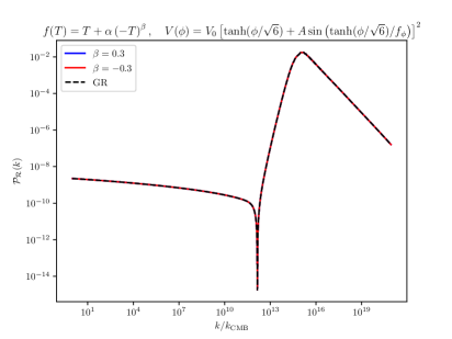
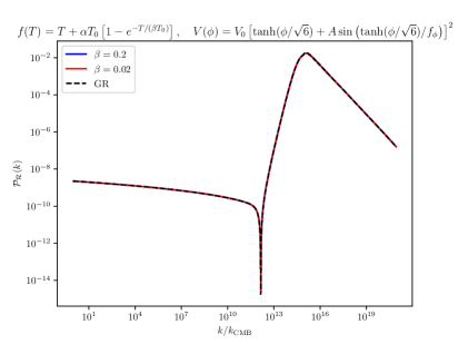
Figure 1: In top panel we show the curvature power spectrum $\mathcal{P}_{\mathcal{R}}(k)$ for the power-law $f(T)$ model for various values of the $\beta$ parameter while in the bottom panel we show $\mathcal{P}_{\mathcal{R}}(k)$ for the exponential $f(T)$ model. The black dashed line stands for $\mathcal{P}_{\mathcal{R}}(k)$ within GR. For all curves we work with the modulated chaotic inflationary potential (47).

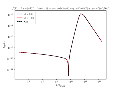
Figure 2: In the top panel we show the curvature power spectrum $\mathcal{P}_{\mathcal{R}}(k)$ for the power-law $f(T)$ model for various values of the $\beta$ parameter while in the bottom panel we show $\mathcal{P}_{\mathcal{R}}(k)$ for the exponential $f(T)$ model. The black dashed line stands for $\mathcal{P}_{\mathcal{R}}(k)$ within GR. For all curves we work with the polynomial superpotential (48).

At this point, we need to highlight that we derived the curvature power spectrum within mono-parametric $f(T)$ gravity theories without non-minimal matter-gravity couplings. One in general would expect a different behaviour in the case where there is a non-minimal coupling between the gravity and the matter sector, namely when $f_{,T\phi}\neq 0$. This intuitive physical condition can be analytically derived from extracting $\mathcal{P}_{\mathcal{R}}(k)$ within the slow-roll regime and checking which are the necessary conditions for the curvature power spectrum within teleparallel gravity to be distinctive from that within GR.

For this reason, let us derive here the $\mathcal{P}_{\mathcal{R}}(k)$ at linear order in the slow roll regime, namely when $\epsilon,\eta\ll 1$, within the framework of $f(T)$ gravity theories . After appropriate approximations (see [127] for more details), we can write

$$\begin{split}\left|\mathcal{R}_{k}\right|\simeq&\frac{H}{2\mathchoice{{\hbox{$\displaystyle\sqrt{k^{3}Q_{s}\,}$}\lower 0.4pt\hbox{\vrule height=8.74889pt,depth=-6.99915pt}}}{{\hbox{$\textstyle\sqrt{k^{3}Q_{s}\,}$}\lower 0.4pt\hbox{\vrule height=8.74889pt,depth=-6.99915pt}}}{{\hbox{$\scriptstyle\sqrt{k^{3}Q_{s}\,}$}\lower 0.4pt\hbox{\vrule height=6.14998pt,depth=-4.92001pt}}}{{\hbox{$\scriptscriptstyle\sqrt{k^{3}Q_{s}\,}$}\lower 0.4pt\hbox{\vrule height=4.7611pt,depth=-3.8089pt}}}}\left(\frac{k}{aH}\right)^{\frac{3}{2}-\tilde{\nu}}\\ &\simeq\frac{H_{k}}{2\mathchoice{{\hbox{$\displaystyle\sqrt{k^{3}Q_{sk}\,}$}\lower 0.4pt\hbox{\vrule height=8.74889pt,depth=-6.99915pt}}}{{\hbox{$\textstyle\sqrt{k^{3}Q_{sk}\,}$}\lower 0.4pt\hbox{\vrule height=8.74889pt,depth=-6.99915pt}}}{{\hbox{$\scriptstyle\sqrt{k^{3}Q_{sk}\,}$}\lower 0.4pt\hbox{\vrule height=6.14998pt,depth=-4.92001pt}}}{{\hbox{$\scriptscriptstyle\sqrt{k^{3}Q_{sk}\,}$}\lower 0.4pt\hbox{\vrule height=4.7611pt,depth=-3.8089pt}}}}\left[1+\eta_{\mathcal{R}}\ln\left(\frac{k}{aH}\right)\right],\end{split}$$ (65)

where $H_{k}$ and $Q_{sk}$ are the values of $H$ and $Q_{s}$ evaluated at horizon crossing time, namely when $k=aH$. Finally, the curvature power spectrum can be recast as

$$\mathcal{P}_{\mathcal{R}}(k)\equiv\frac{k^{3}}{2\pi^{2}}\left|\mathcal{R}_{k}(\tau)\right|^{2}\simeq\frac{H_{k}^{2}}{8\pi^{2}Q_{sk}}\left[1+2\eta_{\mathcal{R}}\ln\left(\frac{k}{aH}\right)\right].$$ (66)

Given that $\eta_{\mathcal{R}}\sim\mathcal{O}(\epsilon)$, one finds that the local Lorentz violation gives rise to a slight logarithmic time-dependence of the curvature perturbation and its power spectrum on superhorizon scales. Finally, the scale-dependence of the curvature power spectrum is quantified in the scalar spectral index $n_{\mathrm{s}}$ defined by

$${n_{\mathrm{s}}-1\equiv\left.\frac{d\ln{\mathcal{P}_{\mathcal{R}}(k)}}{d\ln{k}}\right|_{k=aH}=-2\epsilon-\eta+2\eta_{\mathcal{R}},}$$ (67)

from which we see the deviation from GR due to the presence of the term $2\eta_{\mathcal{R}}$, which carries the effects of the local Lorentz violation.

Finally, one can show that $\eta_{\mathcal{R}}$ can be recast in the following form:

$$\eta_{\mathcal{R}}=(\delta_{fX}-2\mu\epsilon)\left[1-\frac{1+2\mu}{(1+2\mu)\epsilon-\delta_{fX}}\frac{\delta_{fX}-2\mu\epsilon}{2\mu}\right].$$ (68)

Interestingly, for $\delta_{fX}=0$, i.e. in the absence of matter-gravity coupling, $\eta_{\mathcal{R}}=-4\mu\epsilon\ll 1$, since $\epsilon<1$ and $\mu=Tf_{,TT}/f_{,T}\ll 1$ for viable $f(T)$ models [109] and $Q_{sk}=\epsilon_{k}$. Thus, in the absence of matter-gravity coupling one obtains that $\mathcal{P}^{f(T)}_{\mathcal{R}}(k)\simeq\mathcal{P}^{\mathrm{GR}}_{\mathcal{R}}(k)$ and consequently can claim that there will be essentially no distinctive deviation between $f(T)$ and GR at the level of the curvature power spectrum.

One therefore should introduce a matter-gravity coupling at the level of the Lagrangian in order to detect a potential deviation from GR at the level of $\mathcal{P}_{\mathcal{R}}(k)$ constituting the source of the SIGWs.

III.3.2 The effect of the gravitational-wave propagation

We now study the effect of the underlying telleparallel gravity theory at the level of the GW propagation. To do so, one should essentially investigate the behavior of the Green function, $G_{k}(\eta,\bar{\eta})$, which can be viewed as the propagator of the tensor perturbations as it can be seen from Eq. (56).

In particular, one must identify the dominant terms in the evolution equation for the Green function Eq. (57), which we write as follows

$$\begin{split}G_{\boldsymbol{k}}^{\lambda,\prime\prime}(\eta,\bar{\eta})-&2\mathcal{H}\gamma_{T}G_{\boldsymbol{k}}^{\lambda,\prime}(\eta,\bar{\eta})+\\ &\left(k^{2}-\frac{a^{\prime\prime}}{a}+2\mathcal{H}^{2}\gamma_{T}\right)G^{\lambda}_{\boldsymbol{k}}(\eta,\bar{\eta})=\delta\left(\eta-\bar{\eta}\right),\end{split}$$ (69)

and take the ratios between the GR terms and the new $f(T)$ terms multiplied by the $\gamma_{T}$ function.

At the end, following the same reasoning as in [122] and accounting for the fact that the $\gamma_{T}$ function in the case of no non-minimal matter-gravity coupling is a negative decreasing function of time, we derive the maximum deviation from GR by extracting the ratios between the GR and $f(T)$ terms at a time during radiation domination when the $\gamma_{T}$ function acquires its maximum value. Being quite conservative, we choose this time as the standard matter-radiation equality time at redshift $z_{\mathrm{eq}}=3387$. Finally, we find that independently of the value of the $f(T)$ gravity parameter $\beta$ one obtains that

$$\begin{split}&\left|\frac{G_{\boldsymbol{k}}^{\prime\prime}(\eta,\bar{\eta})}{2\mathcal{H}\gamma_{T}G_{\boldsymbol{k}}^{\prime}(\eta,\bar{\eta})}\right|\simeq\left.\frac{1}{2\mathcal{H}\gamma_{T}}\right|_{\eta=\eta_{\mathrm{eq}}}\gg 1\quad\mathrm{and}\\ &\left.\frac{k^{2}}{2\mathcal{H}^{2}\gamma_{T}}\right|_{k=k_{\mathrm{evap}},\eta=\eta_{\mathrm{eq}}}\gg 1,\end{split}$$ (70)

where $k_{\mathrm{evap}}$ is the comoving scale exiting the Hubble radius at PBH evaporation time, thus being the largest scale considered here.

In summary, we can safely argue that the modifications of any modified teleparallel gravity theory with no non-minimal gravity-matter coupling at the level of the GW propagation equation (69) are negligible. As a consequence, one concludes that

$$G_{\boldsymbol{k}}^{f(T)}(\eta,\bar{\eta})\simeq G_{\boldsymbol{k}}^{\mathrm{GR}}(\eta,{\bar{\eta}}),\quad\mathrm{with}\quad f_{,T\phi}=0.$$ (71)

One then needs to introduce a coupling between gravity and matter in order to see a distinctive deviation from GR.

IV Conclusions

Primordial black holes are of great significance, since they can naturally address many issues of modern cosmology, among them the dark matter problem and the generation of large-scale structures. Interestingly, they are associated with numerous GW signals from GWs from PBH mergers up to primordial GWs of cosmological origin related to their formation.

In particular, the enhanced cosmological perturbations which collapse to form PBHs can induce a stochastic gravitational-wave background due to second-order gravitational interactions. This GW portal was mainly studied within classical gravity while in some early works in this research area it was shown that it can as well serve as a novel probe to test and constrain alternative gravity theories.

In this work, we studied the aforementioned GW signal within the context of modified teleparallel gravity theories where the gravitational Lagrangian is a function of the torsion scalar $T$. Interestingly enough, we showed that in the absence of explicit non-minimal couplings between gravity and matter sectors, the effect of the underlying modified theory of gravity at the level of the source and the propagation of the GWs is practically negligible, leading to an indistinguishable SIGW signal compared to that within GR. Additionally, we would like to mention here that a similar indistinguishable GW signal compared to GR was found as well regarding the GW portal associated to PBH Poisson fluctuations within teleparallel theories of gravity [122].

Finally, it is important to highlight that one needs to introduce a non-minimal matter-gravity couplings in order to observe a distinctive SIGW signal compared to GR. Furthermore, it would be illuminating to extract the induced GW signal within other modified gravity theories, namely within $f(R)$ and $f(Q)$ gravity theories, in order to potentially test and constrain the underlying theory of gravity. These studies will be performed in upcoming projects.

Appendix A The power-law $f(T)$ model

A.1 Background equations

For the power-law $f(T)$ model (43), after assuming homogeneity and isotropy of the scalar field (hence $X=\dot{\phi}^{2}/2$) and working with the e-fold number defined as the logarithm of the scale factor, i.e. $N\equiv\ln a$, Eqs. (17), (18) and (19) become

$$\frac{TM_{\scriptscriptstyle{\mathrm{Pl}}}^{2}}{2}+\frac{T^{\beta}M_{\scriptscriptstyle{\mathrm{Pl}}}^{2}\alpha(2\beta-1)}{2}-\frac{H^{2}\phi^{\prime 2}}{2}-V=0,$$ (72)

$$\begin{split}\frac{TM_{\scriptscriptstyle{\mathrm{Pl}}}^{2}}{2}+&\frac{T^{\beta}M_{\scriptscriptstyle{\mathrm{Pl}}}^{2}\alpha(2\beta-1)}{2}+\frac{H^{2}\phi^{\prime 2}}{2}-V-2\epsilon H^{2}M_{\scriptscriptstyle{\mathrm{Pl}}}^{2}\\ &-2\epsilon H^{2}M_{\scriptscriptstyle{\mathrm{Pl}}}^{2}\alpha\beta\left[T^{\beta-1}+(\beta-1)HT^{\beta-2}T^{\prime}\right]=0\end{split}$$ (73)

$$\phi^{\prime\prime}+(3-\epsilon)\phi^{\prime}+V_{,\phi}/H^{2}=0$$ (74)

where $\prime$ denotes derivative with respect to the e-fold number, $\epsilon=-H^{\prime}/H$, $T=6H^{2}$ and $T^{\prime}=12HH^{\prime}$.

A.2 Mukhanov - Sasaki equation

We need to solve these equations together with the Mukhanov - Sasaki equation (36). Working again with the e-fold number as time variable one obtains from Eq. (36) that

$$\mathcal{R}^{\prime\prime}+\left(1-\epsilon+2\frac{z^{\prime}}{z}\right)\mathcal{R}^{\prime}+\left(\frac{k^{2}}{H^{2}a^{2}}+\frac{m^{2}}{H^{2}}\right)\mathcal{R}=0,$$ (75)

with

$$\frac{z^{\prime}}{z}=1+\phi^{\prime\prime}/\phi^{\prime},\,\,\,\,\epsilon=\frac{{\phi^{\prime}}^{2}/(2M_{pl}^{2})}{1+\alpha\beta(2\beta-1)T^{\beta-1}}.$$ (76)

The expression for $m^{2}$ will read as

$$m^{2}=3H^{2}\eta_{\mathcal{R}}=-72H^{4}\frac{\alpha\beta(\beta-1)(6H^{2})^{\beta-2}\epsilon}{1+\alpha\beta(6H^{2})^{\beta-1}}.$$ (77)

Appendix B The exponential $f(T)$ model

B.1 Background equations

For exponential model (45), following the same procedure as before (hence $X=\dot{\phi}^{2}/2$) and working with the e-fold number as the time variable equations (17), (18) and (19) become

$$\begin{split}3H^{2}M_{\scriptscriptstyle{\mathrm{Pl}}}^{2}-3H_{0}^{2}M_{\scriptscriptstyle{\mathrm{Pl}}}^{2}\alpha\left(1-e^{-\frac{H^{2}}{\beta H_{0}^{2}}}\right)&+\frac{6H^{2}M_{\scriptscriptstyle{\mathrm{Pl}}}^{2}\alpha}{\beta}e^{\frac{-H^{2}}{\beta H_{0}^{2}}}\\ &-\frac{\phi^{\prime 2}H^{2}}{2}-V=0\end{split}$$ (78)

$$\begin{split}3H^{2}M_{\scriptscriptstyle{\mathrm{Pl}}}^{2}&-3H_{0}^{2}M_{\scriptscriptstyle{\mathrm{Pl}}}^{2}\alpha\left(1-e^{-\frac{H^{2}}{\beta H_{0}^{2}}}\right)+\frac{6H^{2}M_{\scriptscriptstyle{\mathrm{Pl}}}^{2}\alpha}{\beta}e^{\frac{-H^{2}}{\beta H_{0}^{2}}}\\ &+\frac{\phi^{\prime 2}H^{2}}{2}-V-2\epsilon H^{2}M_{\scriptscriptstyle{\mathrm{Pl}}}^{2}\left(1+\frac{\alpha}{\beta}e^{\frac{-H^{2}}{\beta H_{0}^{2}}}\right)\\ &+4H^{2}M_{\scriptscriptstyle{\mathrm{Pl}}}^{2}e^{\frac{-H^{2}}{\beta H_{0}^{2}}}\frac{\alpha\epsilon H^{2}}{\beta^{2}H_{0}^{2}}=0\end{split}$$ (79)

$$\phi^{\prime\prime}+(3-\epsilon)\phi^{\prime}+\frac{V_{,\phi}}{H^{2}}=0.$$ (80)

B.2 Mukhanov - Sasaki equation

Once again, regarding the MS equation one should solve the following equation for the comoving curvature perturbation $\mathcal{R}$:

$$\mathcal{R}^{\prime\prime}+\left(1-\epsilon+2\frac{z^{\prime}}{z}\right)\mathcal{R}^{\prime}+\left(\frac{k^{2}}{H^{2}a^{2}}+\frac{m^{2}}{H^{2}}\right)\mathcal{R}=0,$$ (81)

with

$$\begin{split}&\frac{z^{\prime}}{z}=1+\phi^{\prime\prime}/\phi^{\prime},\quad\epsilon=\frac{{\phi^{\prime}}^{2}/(2M_{pl}^{2})}{1+\alpha\beta(2\beta-1)T^{\beta-1}},\quad\\ &m^{2}=-12H^{2}\frac{\epsilon\alpha H^{2}e^{\frac{-H^{2}}{\beta H_{0}^{2}}}}{\beta^{2}H_{0}^{2}\left(1+\frac{\alpha}{\beta}e^{\frac{-H^{2}}{\beta H_{0}^{2}}}\right)}.\end{split}$$ (82)

References

- [1] Y. B. Zel’dovich and I. D. Novikov, The Hypothesis of Cores Retarded during Expansion and the Hot Cosmological Model, Soviet Astronomy 10 (Feb., 1967) 602.
- [2] B. J. Carr and S. W. Hawking, Black holes in the early Universe, Mon. Not. Roy. Astron. Soc. 168 (1974) 399–415.
- [3] B. J. Carr, The primordial black hole mass spectrum, ApJ 201 (Oct., 1975) 1–19.
- [4] G. F. Chapline, Cosmological effects of primordial black holes, Nature 253 (1975) 251–252.
- [5] S. Clesse and J. García-Bellido, Seven Hints for Primordial Black Hole Dark Matter, Phys. Dark Univ. 22 (2018) 137–146, [1711.10458].
- [6] P. Meszaros, Primeval black holes and galaxy formation, Astron. Astrophys. 38 (1975) 5–13.
- [7] N. Afshordi, P. McDonald and D. Spergel, Primordial black holes as dark matter: The Power spectrum and evaporation of early structures, Astrophys. J. Lett. 594 (2003) L71–L74, [astro-ph/0302035].
- [8] B. Carr, K. Kohri, Y. Sendouda and J. Yokoyama, Constraints on Primordial Black Holes, 2002.12778.
- [9] M. Sasaki, T. Suyama, T. Tanaka and S. Yokoyama, Primordial black holes—perspectives in gravitational wave astronomy, Class. Quant. Grav. 35 (2018) 063001, [1801.05235].
- [10] Z. Zhou, J. Jiang, Y.-F. Cai, M. Sasaki and S. Pi, Primordial black holes and gravitational waves from resonant amplification during inflation, Phys. Rev. D 102 (2020) 103527, [2010.03537].
- [11] T. Nakamura, M. Sasaki, T. Tanaka and K. S. Thorne, Gravitational waves from coalescing black hole MACHO binaries, Astrophys. J. 487 (1997) L139–L142, [astro-ph/9708060].
- [12] K. Ioka, T. Chiba, T. Tanaka and T. Nakamura, Black hole binary formation in the expanding universe: Three body problem approximation, Phys. Rev. D58 (1998) 063003, [astro-ph/9807018].
- [13] I. Zaballa, A. M. Green, K. A. Malik and M. Sasaki, Constraints on the primordial curvature perturbation from primordial black holes, JCAP 0703 (2007) 010, [astro-ph/0612379].
- [14] M. Raidal, V. Vaskonen and H. Veermäe, Gravitational Waves from Primordial Black Hole Mergers, JCAP 1709 (2017) 037, [1707.01480].
- [15] E. Cotner, A. Kusenko, M. Sasaki and V. Takhistov, Analytic Description of Primordial Black Hole Formation from Scalar Field Fragmentation, JCAP 10 (2019) 077, [1907.10613].
- [16] E. Bugaev and P. Klimai, Induced gravitational wave background and primordial black holes, Phys. Rev. D 81 (2010) 023517, [0908.0664].
- [17] R. Saito and J. Yokoyama, Gravitational-wave background as a probe of the primordial black-hole abundance, Physical Review Letters 102 (Apr, 2009) .
- [18] T. Nakama and T. Suyama, Primordial black holes as a novel probe of primordial gravitational waves, Physical Review D 92 (Dec, 2015) .
- [19] G. Domènech, Scalar Induced Gravitational Waves Review, Universe 7 (2021) 398, [2109.01398].
- [20] T. Papanikolaou, V. Vennin and D. Langlois, Gravitational waves from a universe filled with primordial black holes, JCAP 03 (2021) 053, [2010.11573].
- [21] G. Domènech, C. Lin and M. Sasaki, Gravitational wave constraints on the primordial black hole dominated early universe, JCAP 04 (2021) 062, [2012.08151].
- [22] T. Papanikolaou, Gravitational waves induced from primordial black hole fluctuations: the effect of an extended mass function, JCAP 10 (2022) 089, [2207.11041].
- [23] H. Li et al., Probing Primordial Gravitational Waves: Ali CMB Polarization Telescope, Natl. Sci. Rev. 6 (2019) 145–154, [1710.03047].
- [24] Y.-F. Cai, C. Chen, X. Tong, D.-G. Wang and S.-F. Yan, When Primordial Black Holes from Sound Speed Resonance Meet a Stochastic Background of Gravitational Waves, Phys. Rev. D 100 (2019) 043518, [1902.08187].
- [25] G. Domènech, S. Pi and M. Sasaki, Induced gravitational waves as a probe of thermal history of the universe, JCAP 08 (2020) 017, [2005.12314].
- [26] Y.-F. Cai, C. Lin, B. Wang and S.-F. Yan, Sound speed resonance of the stochastic gravitational wave background, Phys. Rev. Lett. 126 (2021) 071303, [2009.09833].
- [27] J. Fumagalli, S. Renaux-Petel and L. T. Witkowski, Oscillations in the stochastic gravitational wave background from sharp features and particle production during inflation, JCAP 08 (2021) 030, [2012.02761].
- [28] J. Fumagalli, G. A. Palma, S. Renaux-Petel, S. Sypsas, L. T. Witkowski and C. Zenteno, Primordial gravitational waves from excited states, JHEP 03 (2022) 196, [2111.14664].
- [29] R.-G. Cai, Z.-K. Guo, J. Liu, L. Liu and X.-Y. Yang, Primordial black holes and gravitational waves from parametric amplification of curvature perturbations, JCAP 06 (2020) 013, [1912.10437].
- [30] R.-G. Cai, S. Pi, S.-J. Wang and X.-Y. Yang, Resonant multiple peaks in the induced gravitational waves, JCAP 05 (2019) 013, [1901.10152].
- [31] G. Domènech, Induced gravitational waves in a general cosmological background, Int. J. Mod. Phys. D 29 (2020) 2050028, [1912.05583].
- [32] M. Maggiore et al., Science Case for the Einstein Telescope, JCAP 03 (2020) 050, [1912.02622].
- [33] C. Caprini et al., Science with the space-based interferometer eLISA. II: Gravitational waves from cosmological phase transitions, JCAP 04 (2016) 001, [1512.06239].
- [34] N. Karnesis et al., The Laser Interferometer Space Antenna mission in Greece White Paper, 2209.04358.
- [35] G. Janssen et al., Gravitational wave astronomy with the SKA, PoS AASKA14 (2015) 037, [1501.00127].
- [36] K. S. Stelle, Renormalization of Higher Derivative Quantum Gravity, Phys. Rev. D 16 (1977) 953–969.
- [37] A. Addazi et al., Quantum gravity phenomenology at the dawn of the multi-messenger era – A review, 2111.05659.
- [38] S. Nojiri and S. D. Odintsov, Unified cosmic history in modified gravity: from F(R) theory to Lorentz non-invariant models, Phys. Rept. 505 (2011) 59–144, [1011.0544].
- [39] J. Martin, C. Ringeval and V. Vennin, Encyclopædia Inflationaris, Phys. Dark Univ. 5-6 (2014) 75–235, [1303.3787].
- [40] CANTATA collaboration, E. N. Saridakis et al., Modified Gravity and Cosmology: An Update by the CANTATA Network, 2105.12582.
- [41] S. Capozziello and M. De Laurentis, Extended Theories of Gravity, Phys. Rept. 509 (2011) 167–321, [1108.6266].
- [42] Y.-F. Cai, S. Capozziello, M. De Laurentis and E. N. Saridakis, f(T) teleparallel gravity and cosmology, Rept. Prog. Phys. 79 (2016) 106901, [1511.07586].
- [43] J. Lin, Q. Gao, Y. Gong, Y. Lu, C. Zhang and F. Zhang, Primordial black holes and secondary gravitational waves from and inflation, Phys. Rev. D 101 (2020) 103515, [2001.05909].
- [44] P. Chen, S. Koh and G. Tumurtushaa, Primordial black holes and induced gravitational waves from inflation in the Horndeski theory of gravity, 2107.08638.
- [45] S. Kawai and J. Kim, Primordial black holes from Gauss-Bonnet-corrected single field inflation, Phys. Rev. D 104 (2021) 083545, [2108.01340].
- [46] J. Lin, S. Gao, Y. Gong, Y. Lu, Z. Wang and F. Zhang, Primordial black holes and scalar induced secondary gravitational waves from Higgs inflation with non-canonical kinetic term, 2111.01362.
- [47] T. Papanikolaou, C. Tzerefos, S. Basilakos and E. N. Saridakis, Scalar induced gravitational waves from primordial black hole Poisson fluctuations in f(R) gravity, JCAP 10 (2022) 013, [2112.15059].
- [48] V. R. Ivanov, S. V. Ketov, E. O. Pozdeeva and S. Y. Vernov, Analytic extensions of Starobinsky model of inflation, JCAP 03 (2022) 058, [2111.09058].
- [49] F. Zhang, Primordial black holes and scalar induced gravitational waves from the E model with a Gauss-Bonnet term, Phys. Rev. D 105 (2022) 063539, [2112.10516].
- [50] Z. Yi, Primordial black holes and scalar-induced gravitational waves from the generalized Brans-Dicke theory, JCAP 03 (2023) 048, [2206.01039].
- [51] D. Y. Cheong, K. Kohri and S. C. Park, The inflaton that could: primordial black holes and second order gravitational waves from tachyonic instability induced in Higgs-R 2 inflation, JCAP 10 (2022) 015, [2205.14813].
- [52] J.-X. Feng, F. Zhang and X. Gao, Scalar induced gravitational waves from Chern-Simons gravity during inflation era, 2302.00950.
- [53] F. Zhang, J.-X. Feng and X. Gao, Circularly polarized scalar induced gravitational waves from the Chern-Simons modified gravity, JCAP 10 (2022) 054, [2205.12045].
- [54] R. Arya, R. K. Jain and A. K. Mishra, Primordial Black Holes Dark Matter and Secondary Gravitational Waves from Warm Higgs-G Inflation, 2302.08940.
- [55] R. Aldrovandi and J. G. Pereira, Teleparallel Gravity: An Introduction. Springer, 2013, 10.1007/978-94-007-5143-9.
- [56] M. Krssak, R. J. van den Hoogen, J. G. Pereira, C. G. Böhmer and A. A. Coley, Teleparallel theories of gravity: illuminating a fully invariant approach, Class. Quant. Grav. 36 (2019) 183001, [1810.12932].
- [57] G. R. Bengochea and R. Ferraro, Dark torsion as the cosmic speed-up, Phys. Rev. D 79 (2009) 124019, [0812.1205].
- [58] E. V. Linder, Einstein’s Other Gravity and the Acceleration of the Universe, Phys. Rev. D 81 (2010) 127301, [1005.3039].
- [59] S.-H. Chen, J. B. Dent, S. Dutta and E. N. Saridakis, Cosmological perturbations in f(T) gravity, Phys. Rev. D 83 (2011) 023508, [1008.1250].
- [60] R. Zheng and Q.-G. Huang, Growth factor in gravity, JCAP 03 (2011) 002, [1010.3512].
- [61] K. Bamba, C.-Q. Geng, C.-C. Lee and L.-W. Luo, Equation of state for dark energy in gravity, JCAP 01 (2011) 021, [1011.0508].
- [62] Y.-F. Cai, S.-H. Chen, J. B. Dent, S. Dutta and E. N. Saridakis, Matter Bounce Cosmology with the f(T) Gravity, Class. Quant. Grav. 28 (2011) 215011, [1104.4349].
- [63] S. Capozziello, V. F. Cardone, H. Farajollahi and A. Ravanpak, Cosmography in f(T)-gravity, Phys. Rev. D 84 (2011) 043527, [1108.2789].
- [64] K. Bamba, S. D. Odintsov and D. Sáez-Gómez, Conformal symmetry and accelerating cosmology in teleparallel gravity, Phys. Rev. D 88 (2013) 084042, [1308.5789].
- [65] J.-T. Li, C.-C. Lee and C.-Q. Geng, Einstein Static Universe in Exponential Gravity, Eur. Phys. J. C 73 (2013) 2315, [1302.2688].
- [66] Y. C. Ong, K. Izumi, J. M. Nester and P. Chen, Problems with Propagation and Time Evolution in f(T) Gravity, Phys. Rev. D 88 (2013) 024019, [1303.0993].
- [67] K. Bamba, G. G. L. Nashed, W. El Hanafy and S. K. Ibraheem, Bounce inflation in Cosmology: A unified inflaton-quintessence field, Phys. Rev. D 94 (2016) 083513, [1604.07604].
- [68] M. Malekjani, N. Haidari and S. Basilakos, Spherical collapse model and cluster number counts in power law gravity, Mon. Not. Roy. Astron. Soc. 466 (2017) 3488–3496, [1609.01964].
- [69] G. Farrugia and J. Levi Said, Stability of the flat FLRW metric in gravity, Phys. Rev. D 94 (2016) 124054, [1701.00134].
- [70] S. Bahamonde, C. G. Böhmer and M. Krššák, New classes of modified teleparallel gravity models, Phys. Lett. B 775 (2017) 37–43, [1706.04920].
- [71] L. Karpathopoulos, S. Basilakos, G. Leon, A. Paliathanasis and M. Tsamparlis, Cartan symmetries and global dynamical systems analysis in a higher-order modified teleparallel theory, Gen. Rel. Grav. 50 (2018) 79, [1709.02197].
- [72] H. Abedi, S. Capozziello, R. D’Agostino and O. Luongo, Effective gravitational coupling in modified teleparallel theories, Phys. Rev. D 97 (2018) 084008, [1803.07171].
- [73] R. D’Agostino and O. Luongo, Growth of matter perturbations in nonminimal teleparallel dark energy, Phys. Rev. D 98 (2018) 124013, [1807.10167].
- [74] D. Iosifidis and T. Koivisto, Scale transformations in metric-affine geometry, Universe 5 (2019) 82, [1810.12276].
- [75] S. Chakrabarti, J. L. Said and K. Bamba, On Reconstruction of Extended Teleparallel Gravity from the Cosmological Jerk Parameter, Eur. Phys. J. C 79 (2019) 454, [1905.09711].
- [76] S. Davood Sadatian, Effects of viscous content on the modified cosmological F(T) model, EPL 126 (2019) 30004.
- [77] S.-F. Yan, P. Zhang, J.-W. Chen, X.-Z. Zhang, Y.-F. Cai and E. N. Saridakis, Interpreting cosmological tensions from the effective field theory of torsional gravity, Phys. Rev. D 101 (2020) 121301, [1909.06388].
- [78] D. Wang and D. Mota, Can gravity resolve the tension?, Phys. Rev. D 102 (2020) 063530, [2003.10095].
- [79] A. Bose and S. Chakraborty, Cosmic evolution in f(T) gravity theory, Mod. Phys. Lett. A 35 (2020) 2050296, [2010.16247].
- [80] X. Ren, T. H. T. Wong, Y.-F. Cai and E. N. Saridakis, Data-driven Reconstruction of the Late-time Cosmic Acceleration with f(T) Gravity, Phys. Dark Univ. 32 (2021) 100812, [2103.01260].
- [81] C. Escamilla-Rivera, G. A. Rave-Franco and J. L. Said, f(T, B) Cosmography for High Redshifts, Universe 7 (2021) 441, [2110.05434].
- [82] V. C. De Andrade, L. C. T. Guillen and J. G. Pereira, Teleparallel gravity: An Overview, in 9th Marcel Grossmann Meeting on Recent Developments in Theoretical and Experimental General Relativity, Gravitation and Relativistic Field Theories (MG 9), 11, 2000. gr-qc/0011087.
- [83] H. I. Arcos and J. G. Pereira, Torsion gravity: A Reappraisal, Int. J. Mod. Phys. D 13 (2004) 2193–2240, [gr-qc/0501017].
- [84] J. G. Pereira and Y. N. Obukhov, Gauge Structure of Teleparallel Gravity, Universe 5 (2019) 139, [1906.06287].
- [85] S. Weinberg, Gravitation and Cosmology: Principles and Applications of the General Theory of Relativity. John Wiley and Sons, New York, 1972.
- [86] R. Aldrovandi and J. G. Pereira, An Introduction to geometrical physics. 1996.
- [87] S. Bahamonde, K. F. Dialektopoulos, C. Escamilla-Rivera, G. Farrugia, V. Gakis, M. Hendry et al., Teleparallel Gravity: From Theory to Cosmology, 2106.13793.
- [88] C.-Q. Geng, C.-C. Lee, E. N. Saridakis and Y.-P. Wu, “Teleparallel” dark energy, Phys. Lett. B 704 (2011) 384–387, [1109.1092].
- [89] G. Otalora, Scaling attractors in interacting teleparallel dark energy, JCAP 07 (2013) 044, [1305.0474].
- [90] G. Otalora, Cosmological dynamics of tachyonic teleparallel dark energy, Phys. Rev. D 88 (2013) 063505, [1305.5896].
- [91] G. Otalora, A novel teleparallel dark energy model, Int. J. Mod. Phys. D 25 (2015) 1650025, [1402.2256].
- [92] M. A. Skugoreva, E. N. Saridakis and A. V. Toporensky, Dynamical features of scalar-torsion theories, Phys. Rev. D 91 (2015) 044023, [1412.1502].
- [93] B. Li, T. P. Sotiriou and J. D. Barrow, Large-scale Structure in f(T) Gravity, Phys. Rev. D 83 (2011) 104017, [1103.2786].
- [94] M. Gonzalez-Espinoza, G. Otalora, J. Saavedra and N. Videla, Growth of matter overdensities in non-minimal torsion-matter coupling theories, Eur. Phys. J. C 78 (2018) 799, [1808.01941].
- [95] M. Gonzalez-Espinoza and G. Otalora, Generating primordial fluctuations from modified teleparallel gravity with local lorentz-symmetry breaking, Physics Letters B 809 (2020) 135696.
- [96] M. Gonzalez-Espinoza, G. Otalora and J. Saavedra, Stability of scalar perturbations in scalar-torsion f(t,) gravity theories in the presence of a matter fluid, Journal of Cosmology and Astroparticle Physics 2021 (oct, 2021) 007.
- [97] T. P. Sotiriou, B. Li and J. D. Barrow, Generalizations of teleparallel gravity and local Lorentz symmetry, Phys. Rev. D 83 (2011) 104030, [1012.4039].
- [98] B. Li, T. P. Sotiriou and J. D. Barrow, gravity and local Lorentz invariance, Phys. Rev. D 83 (2011) 064035, [1010.1041].
- [99] M. Krššák and E. N. Saridakis, The covariant formulation of f(T) gravity, Class. Quant. Grav. 33 (2016) 115009, [1510.08432].
- [100] A. De Felice and S. Tsujikawa, f(R) theories, Living Rev. Rel. 13 (2010) 3, [1002.4928].
- [101] Y.-P. Wu and C.-Q. Geng, Primordial Fluctuations within Teleparallelism, Phys. Rev. D 86 (2012) 104058, [1110.3099].
- [102] A. De Felice and S. Tsujikawa, Inflationary non-Gaussianities in the most general second-order scalar-tensor theories, Phys. Rev. D 84 (2011) 083504, [1107.3917].
- [103] K. Izumi and Y. C. Ong, Cosmological Perturbation in f(T) Gravity Revisited, JCAP 06 (2013) 029, [1212.5774].
- [104] A. Golovnev and T. Koivisto, Cosmological perturbations in modified teleparallel gravity models, JCAP 11 (2018) 012, [1808.05565].
- [105] R. Bluhm and V. A. Kostelecký , Spontaneous lorentz violation, nambu-goldstone modes, and gravity, Physical Review D 71 (mar, 2005) .
- [106] R. Bluhm, S.-H. Fung and V. A. Kostelecký , Spontaneous lorentz and diffeomorphism violation, massive modes, and gravity, Physical Review D 77 (mar, 2008) .
- [107] D. Baumann, Cosmology. Cambridge University Press, 2022, 10.1017/9781108937092.
- [108] J. M. Maldacena, Non-Gaussian features of primordial fluctuations in single field inflationary models, JHEP 05 (2003) 013, [astro-ph/0210603].
- [109] S. Nesseris, S. Basilakos, E. N. Saridakis and L. Perivolaropoulos, Viable models are practically indistinguishable from CDM, Phys. Rev. D 88 (2013) 103010, [1308.6142].
- [110] R. C. Nunes, S. Pan and E. N. Saridakis, New observational constraints on gravity through gravitational-wave astronomy, Phys. Rev. D 98 (2018) 104055, [1810.03942].
- [111] F. K. Anagnostopoulos, S. Basilakos and E. N. Saridakis, Bayesian analysis of gravity using data, Phys. Rev. D 100 (2019) 083517, [1907.07533].
- [112] I. Dalianis, A. Kehagias and G. Tringas, Primordial black holes from -attractors, JCAP 01 (2019) 037, [1805.09483].
- [113] R. Kallosh and A. Linde, New models of chaotic inflation in supergravity, JCAP 11 (2010) 011, [1008.3375].
- [114] K. N. Ananda, C. Clarkson and D. Wands, The Cosmological gravitational wave background from primordial density perturbations, Phys. Rev. D75 (2007) 123518, [gr-qc/0612013].
- [115] D. Baumann, P. J. Steinhardt, K. Takahashi and K. Ichiki, Gravitational Wave Spectrum Induced by Primordial Scalar Perturbations, Phys. Rev. D76 (2007) 084019, [hep-th/0703290].
- [116] K. Kohri and T. Terada, Semianalytic calculation of gravitational wave spectrum nonlinearly induced from primordial curvature perturbations, Phys. Rev. D97 (2018) 123532, [1804.08577].
- [117] J. R. Espinosa, D. Racco and A. Riotto, A Cosmological Signature of the SM Higgs Instability: Gravitational Waves, JCAP 1809 (2018) 012, [1804.07732].
- [118] V. De Luca, G. Franciolini, A. Kehagias and A. Riotto, On the Gauge Invariance of Cosmological Gravitational Waves, JCAP 03 (2020) 014, [1911.09689].
- [119] C. Yuan, Z.-C. Chen and Q.-G. Huang, Scalar induced gravitational waves in different gauges, Phys. Rev. D 101 (2020) 063018, [1912.00885].
- [120] K. Inomata and T. Terada, Gauge Independence of Induced Gravitational Waves, Phys. Rev. D 101 (2020) 023523, [1912.00785].
- [121] D. Jeong, J. Pradler, J. Chluba and M. Kamionkowski, Silk damping at a redshift of a billion: New limit on small-scale adiabatic perturbations, Phys. Rev. Lett. 113 (Aug, 2014) 061301.
- [122] T. Papanikolaou, C. Tzerefos, S. Basilakos and E. N. Saridakis, No constraints for f(T) gravity from gravitational waves induced from primordial black hole fluctuations, Eur. Phys. J. C 83 (2023) 31, [2205.06094].
- [123] V. F. Mukhanov, H. A. Feldman and R. H. Brandenberger, Theory of cosmological perturbations. Part 1. Classical perturbations. Part 2. Quantum theory of perturbations. Part 3. Extensions, Phys. Rept. 215 (1992) 203–333.
- [124] M. Maggiore, Gravitational wave experiments and early universe cosmology, Phys. Rept. 331 (2000) 283–367, [gr-qc/9909001].
- [125] R. A. Isaacson, Gravitational Radiation in the Limit of High Frequency. II. Nonlinear Terms and the Ef fective Stress Tensor, Phys. Rev. 166 (1968) 1272–1279.
- [126] C. T. Byrnes and P. S. Cole, Lecture notes on inflation and primordial black holes, 12, 2021. 2112.05716.
- [127] M. Gonzalez-Espinoza and G. Otalora, Generating primordial fluctuations from modified teleparallel gravity with local Lorentz-symmetry breaking, Phys. Lett. B 809 (2020) 135696, [2005.03753].