Propagation and Fluxes of Ultra High Energy Cosmic Rays in $f(R)$ Gravity Theory

Abstract

Even though the sources of the ultra high energy cosmic rays (UHECRs) are yet to be known clearly, the high-quality data collected by the most recent CRs observatories signal that the sources of these CRs should be of the extragalactic origin. As the intergalactic mediums are thought to be filled with the turbulent magnetic fields (TMFs), these intergalactic magnetic fields may have a significant impact on how UHECRs travel across the Universe, which is currently expanding with acceleration. Thus the inclusion of these points in the theory is crucial for understanding the experimental findings on UHECRs. Accordingly, in this work we study the effect of diffusion of UHE particles in presence of TMFs in the light of $f(R)$ theory of gravity. The $f(R)$ theory of gravity is a successful modified theory of gravity in explaining the various aspects of the observable Universe including its current state of expansion. For this work we consider two most studied $f(R)$ gravity models, viz., the power-law model and the Starobinsky model. With these two models we study the diffusive character of propagation of UHECR protons in terms of their density enhancement. The Greisen-Zatsepin-Kuzmin (GZK) cutoff, the dip and the bump are all spectrum characteristics that UHE extragalactic protons acquire when they propagate through the cosmic microwave background (CMB) radiation in presence of TMFs. We analyse all these characteristics through the diffusive flux as well as its modification factor. Model dependence of the modification factor is minimal compared to the diffusive flux. We compare the UHECR protons spectra that are calculated for the considered $f(R)$ gravity models with the available data of the AKENO-AGASA, HiRes, AUGER and YAKUTSK experiments of UHECRs. We see that both the models of $f(R)$ gravity provide the energy spectra of UHECRs with all experimentally observed features, which lay well within the range of combine data of all experiments throughout the energy range of concern, in contrast to the case of the $\Lambda$CDM model.

I Introduction

The discovery of cosmic rays (CRs) by V. F. Hess in 1912 [1] is one of the most significant milestones in the history of modern physics. CRs are charged ionizing particles, mostly consisting of protons, helium, carbon and other heavy ions upto iron emanating from outer space. Although the discovery of CRs has passed more than a hundred and ten years now, the origin, acceleration and propagation mechanisms of CRs are still not clearly known [2, 3, 4], especially in the higher energy range i.e. the energy range $E\geq 0.1$ EeV ($1$ EeV = $10^{18}$ eV). The sources of such usually referred ultra high energy CRs (UHECRs) are not established yet [5, 6, 7, 8]. However, in the energy range $E\leq 0.1$ EeV, it is assumed that the sources are of galactic origin and they are accelerated with supernova explosion [9], while that of the well above this range ($\sim 1$ EeV and above) are of most probably the extragalactic in origin and plausibly to accelerate in gamma ray ($\gamma$-ray) bursts or in active galaxies [2].

The energy spectrum of CRs has an extraordinary range of energies. It extends from about many orders of GeV energies upto $100$ EeV and it exhibits the power-law spectrum. There is a small spectral break known as the knee at about $4$ PeV ($1$ PeV = $10^{15}$ eV) and a flattening at the ankle at about $5$ EeV. In this spectrum, a strong cutoff near $50$ EeV, which is called the GZK (Greisen, Zatsepin and Kuzmin) cutoff [10, 11] is appeared due to the interaction with cosmic microwave background (CMB) photons. Besides this, there are two other signatures also in the spectrum, viz. dip and bump [12, 13, 14, 15]. The first one is due to the pair production ($P+\gamma_{\text{CMB}}\rightarrow e^{+}+e^{-}+P$) and second one is due to the photopion production ($P+\gamma_{\text{CMB}}\rightarrow\pi+N$) with the CMB photons.

The intergalactic medium (IGM) contains turbulent magnetic fields (TMFs), which impact significantly on the propagation of extragalactic UHECRs. In the presence of any random magnetic field, the propagation of a charged particle depends on how much distance is travelled by that particle compared with the scattering length $\lambda=3D/c$ in the medium, where $D$ denotes the diffusion coefficient and $c$ is the speed of light in free space [16]. If the travelled distance of the charge particle is very smaller than the scattering length, then the propagation is ballistic in nature while that is diffusive if the distance is very larger than the scattering length. Consideration of an extragalactic TMF and also taking into account the finite density of sources in the study of propagation of UHECRs may result in a low-energy magnetic horizon effect, which may allow the observations to be consistent with a higher spectral index [9, 17, 18], closer to the values anticipated from diffusive shock acceleration. Other hypothesis rely on the assumption of acceleration of heavy nuclei by extragalactic sources, which then interact with the infrared radiation present in those environments to photodisintegration, producing a significant number of secondary nucleons that might explain the light composition seen below the ankle [19, 20]. In the presence of an intergalactic magnetic field, the propagation of UHECRs can be studied from the Boltzmann transport equation or by using some simulation methods. In Ref. [16], the author presents a system of partial differential equations to describe the propagation of UHCRs in presence of a random magnetic field. In this paper, the author considered the Boltzmann transport equation and obtained the partial differential equations for the number density as well as for the flux of particles. A diffusive character of propagation of CRs is also obtained in this paper. In Ref. [21] (see also Ref. [22]), an astrophysical simulation framework is proposed for studying the propagating extraterrestrial UHE particles. In their work, authors presented a new and upper version of publicly available code CRPropa 3. It is a code for the efficient development of astrophysical predictions for UHE particles. Ref. [23] presented an analytical solution of the diffusion equation for high energy CRs in the expanding Universe. A fitting to the diffusion coefficient $D(E)$ obtained from numerical integration was presented in Ref. [2] for the both Kolmogorov and Kraichnan turbulence. Authors of Ref. [3] studied the effects of diffusion of CRs in the magnetic field of the local supercluster on the UHECRs from a nearby extragalactic source. In this study authors found that a strong enhancement at certain energy ranges of the flux can help to explain the features of CR spectrum and the composition in detail. In Ref. [5], the authors demonstrated the energy spectra of UHECRs as observed by Fly’s Eye [24], HiRes [25], Yakutsk and AGASA [26] from the idea of the UHE proton’s interaction with CMB photons. A detailed analytical study of the propagation of UHE particles in extragalactic magnetic fields has been performed in Ref. [27] by solving the diffusion equation analytically with the energy losses that are to be taken into account. In another study [28], the authors obtained the dip, bump and GZK cutoff in terms of the modification factor, which arise due to various energy losses suffered by CR particles while propagting through the complex galactic or intergalactic space [4]. Similarly, in Ref. [29], authors obtained four features in the CR proton spectrum, viz. the bump, dip, second dip and the GZK cutoff taking into consideration of extragalactic proton’s interaction with CMB and assuming of resulting power-law spectrum.
The General Relativity (GR) developed by Albert Einstein in 1915 to describe the ubiquitous gravitational interaction is the most beautiful, well tested and successful theory in this regard. The discovery of Gravitational Waves (GWs) by LIGO detectors in 2015 [30] after almost hundred years of their prediction by Einstein himself and the release of the first image of supermassive black hole at the centre of the elliptical supergiant galaxy M$87$ by the Event Horizon Telescope (EHT) in 2019 [31, 32, 33, 34, 35, 36] are the robust supports amongst others in a century to GR. Even though the GR has been suffering from many drawbacks from the theoretical as well as observational fronts. For example, the complete quantum theory of GR has remained elusive till now. The most important limitations of GR from the observational point of view are that it can not explain the observed current accelerated expansion [37, 38, 39, 40] of the Universe, and the rotational dynamics of galaxies indicating the missing mass [41] in the Universe. Consequently, the Modified Theories of Gravity (MTGs) have been developed as one of the ways to explain these observed cosmic phenomena, wherein these phenomena are looked at as some special geometrical manifestations of spacetime, which were remained to be taken into account in GR. The most simplest but remarkable and widely used MTG is the $f(R)$ [42] theory of gravity, where the Ricci scalar $R$ in the Einstein-Hilbert (E-H) action is replaced by a function $f(R)$ of $R$. Various models of $f(R)$ gravity theory have been developed so far from different perspectives. Some of the viable as well as famous or popular models of $f(R)$ gravity are the Starobinsky model [43], Hu-Sawicki model [44], Tsujikawa model [45], power-law model [46] etc.
Till now a number of authors have studied the propagation of CRs in the domain of GR [2, 3, 4, 5, 6, 7, 8, 9, 13, 14, 15, 16, 27, 28, 29, 47]. The enhancement of the flux of CRs is obtained in the framework of the $\Lambda$CDM model by a variety of authors [3, 48]. Besides these, differential flux as well as the modification factor have also been studied [4, 5, 13, 16, 27, 28, 29]. Since MTGs have made significant contributions in the understanding the cosmological [49, 50] and astrophysical [51] issues in recent times, it would be wise to apply the MTGs in the field of CRs to study the existing issues in this field. Keeping this point in mind, in this work, we study for the very first time the propagation of UHECRs and their consequent flux in the light of a MTG, the $f(R)$ theory of gravity. For this purpose, we consider two $f(R)$ gravity models, viz. the power-law model [46] and the Starobinsky model [67]. Considering these two models, we have calculated the expression for the number density of particles. From the number density, we have calculated the enhancement factor as well as differential flux and modification factor for the UHECRs.
The remaining part of the paper is arranged as follows. In section II, we discuss the turbulent magnetic field and diffusive propagation mechanism. The basic cosmological equation that is used to calculate the cosmological parameters is introduced in the section III. In section IV, we define $f(R)$ gravity models of our interest and calculate the required model parameters for those models. A fit to these models is also shown in this section in comparison with the observational data. In section V, we calculate the number density of particles and hence the enhancement factor. Here the differential flux and modification factor for the both two models are calculated and are compared the results with AKENO-AGASA [52, 53], HiRes [54], AUGER [55, 56] and YAKUTSK [57] arrays data. Finally, we compare the results for the $\Lambda$CDM, power-law and Starobinsky models and then conclude our paper with a fruitful discussion in section VI.

II Propagation of Cosmic Rays in turbulent magnetic fields

It is a challenging task to build a model for the extragalactic magnetic fields since there are few observable constraints on them [58]. Their exact amplitude values are unknown, and they probably change depending on the region of space being considered. In the cluster centre regions, the large-scale magnetic fields have recorded amplitudes that vary from a few to tens of $\mu$G [59]. Smaller strengths are anticipated in the vacuum regions, with the typical boundaries in unclustered regions being $1$ to $10$ nG. This means that considerable large-scale magnetic fields should also be present in the filaments and sheets of cosmic structures. The evolution of primordial seeds impacted by the process of structure building may result in TMFs in the Universe [2]. As a result, magnetic fields are often connected with the matter density and are therefore stronger in dense areas like superclusters and weaker in voids. In the local supercluster region, a pragmatic estimation place the coherence length of the magnetic fields between $10$ kpc and $1$ Mpc, while their root mean square (rms) strength lies in the range of $1$ to $100$ nG [59, 60, 61]. The regular component of the galactic magnetic field (GMF), which typically has a strength of only a few $\mu$G, may have an impact on the CRs’ arrival directions, but due to its much lesser spatial extent, it is anticipated to have a subdominant impact on the CRs spectrum.

In the local supercluster region, the rotation measure of polarised background sources has suggested the presence of a strong magnetic field, with a potential strength of $0.3$ to $2$ $\mu$G [60]. It is the magnetic field within the local supercluster that is most relevant since the impacts of the magnetic horizon become noticeable when the CRs from the closest sources reach the Earth. Thus we will not consider here the larger scale inhomogeneities from filaments and voids. The propagation of CRs in an isotropic, homogenous, turbulent extragalactic magnetic field will then be simplified. The rms amplitude of magnetic fields $B$ and the coherence length $l_{c}$, which depicts the maximum distance between any two points upto which the magnetic fields correlate with each other, can be used to characterise such magnetic fields. The rms strength of the magnetic fields can be defined as $B=\sqrt{\langle B^{2}(x)\rangle}$, which can take values from $1$ nG upto $100$ nG and that of the coherence length $l_{c}$ can take the values from $0.01$ Mpc to $1$ Mpc.

An effective Larmor radius for charged particles of charge $Ze$ moving with energy $E$ through a TMF of strength $B$ may be defined as

$$r_{L}=\frac{E}{ZeB}\simeq 1.1\frac{E/\text{EeV}}{ZB/\text{nG}}\;\text{Mpc}.$$ (1)

A pertinent quantity in the study of diffusion of charged particles in magnetic fields is the critical energy of the particles. This energy can be defined as the energy at which the coherence length of a particle with charge $Ze$ is equal to its Larmor radius i.e., $r_{L}(E_{c})=l_{c}$ and it is given by

$$E_{c}=ZeBl_{c}\simeq 0.9Z\,\frac{B}{\text{nG}}\,\frac{l_{c}}{\text{Mpc}}\;\text{EeV}.$$ (2)

This energy distinguishes between the regime of resonant diffusion that occurs at low energies ($<E_{c}$) and the non-resonant regime at higher energies ($>E_{c}$). In the resonant diffusion regime the particles suffer large deflections due the interaction with magnetic field $B$ with scales that are comparable to $l_{c}$, whereas in the latter scenario, deflections are small and can only take place across the travel lengths that are greater than $l_{c}$. Extensive numerical simulations of proton’s propagation yielded a fit to the diffusion coefficient $D$ as a function of energy [2], which is given by

$$D(E)\simeq\frac{c\,l_{c}}{3}\left[4\left(\frac{E}{E_{c}}\right)^{2}+a_{I}\left(\frac{E}{E_{c}}\right)+a_{L}\left(\frac{E}{E_{c}}\right)^{2-m}\right],$$ (3)

where $m$ is the index parameter, $a_{I}$ and $a_{L}$ two coefficients. For the case of TMF with Kolmogorov spectrum $m=5/3$ and the coefficients are $a_{L}\approx 0.23$ and $a_{I}\approx 0.9$, while that for Kraichnan spectrum one will have $m=3/2$, $a_{L}\approx 0.42$ and $a_{I}\approx 0.65$. The diffusion length $l_{D}$ relates to the distance after which the particles’ overall deflection is nearly one radian and is given by $l_{D}=3D/c$. From Eq. (3), it is seen that for $E/E_{c}\ll 0.1$ the diffusion length, $l_{D}\simeq a_{L}l_{c}(E/E_{c})^{2-m}$ while that for $E/E_{c}\gg 0.2$, the diffusion length will be $l_{D}\simeq 4\,l_{c}(E/E_{c})^{2}$.

III Basic Cosmological Equations

On a large scale, the Universe appears to be isotropic and homogeneous everywhere. In light of this, the simplest model to be considered is a spatially flat Universe, which is described by the Friedmann-Lemaître-Robertson-Walker (FLRW) metric and it is defined as

$$ds^{2}=-\,dt^{2}+a^{2}(t)\delta_{ij}dx^{i}dx^{j},$$ (4)

where $a(t)$ is the scale factor, $\delta_{ij}$ is the Kronecker delta function with $i,j=\{1,2,3\}$ and $x^{\mu}=\{x^{0},x^{1},x^{2},x^{3}\}$ are comoving coordinates with $x^{0}=t$. Moreover, as a source of curvature we consider the perfect fluid model of the Universe with energy density $\rho$ and pressure $p$ which is specified by the energy-momentum tensor $T^{\mu}_{\nu}=diag(-\,\rho,p,p,p)$. Here we are firstly interested in the basic cosmological evolution equation to be used in our study and this equation is the Friedmann equation. The Friedmann equation in $f(R)$ gravity theory we used is derived by following the Palatini variational approach of the theory. In this approach both the metric $g_{\mu\nu}$ and the torsion-free connection $\Gamma_{\mu\nu}^{\lambda}$ are considered as independent variables. In our present case the metric is $g_{\mu\nu}=diag(-\,1,a^{2},a^{2},a^{2})$ and the connection can be obtained from the $f(R)$ gravity field equations in the Palatini formalism [42]. Following the Palatini formalism the generalized Friedmann equation for our Universe in terms of redshift in $f(R)$ gravity theory can be expressed as [62]

$$\frac{H^{2}}{H_{0}^{2}}=\frac{3\,\Omega_{m0}(1+z)^{3}+6\,\Omega_{r0}(1+z)^{4}+\frac{f(R)}{H_{0}^{2}}}{6f_{R}\zeta^{2}},$$ (5)

where

$$\zeta=1+\frac{9f_{RR}}{2f_{R}}\frac{H_{0}^{2}\,\Omega_{m0}(1+z)^{3}}{Rf_{RR}-f_{R}}.$$ (6)

In Eqs. (5) and (6), $H_{0}\approx 67.4$ kms^-1 Mpc^-1 [63] is the Hubble constant, $\Omega_{m0}\approx 0.315$ [63] is the present value of the matter density parameter and $\Omega_{r0}\approx 5.373\times 10^{-5}$ [64] is the present value of the radiation density parameter. $f_{R}$ and $f_{RR}$ are the first and second order derivatives of the function $f(R)$ with respect to $R$. It is seen that Eqs. (5) and (6) are $f(R)$ gravity model dependent.

Secondly, in our study it is important to know how the cosmological redshift is related with the cosmological time evolution. This can be studied from the connection between the redshift and cosmological time evolution, which is given by

$$\bigg{|}\frac{dt}{dz}\bigg{|}=\frac{1}{(1+z)H}.$$ (7)

The expression of the Hubble parameter $H(z)$ for different models of $f(R)$ gravity will be derived using Eqs. (5) and (6) in the following section IV.

IV $f(R)$ gravity models and cosmological evolution

In this section, we will introduce the power-law model [46] and Starobinsky model [67] of $f(R)$ theory of gravity, and then will derive the expressions for the Hubble parameter and evolution Eq. (7) for these two models. The least square fit to the derived Hubble parameter from the both models with the recent observational data to constrain the model parameters will also be done here. Moreover, the likelihood fit method will be used here to further constrain different model parameters with the observed cosmological data.

IV.1 Power law model and cosmological equations

The general $f(R)$ gravity power-law model is given by [65, 66]

$$f(R)=\lambda\,R^{n},$$ (8)

where $\lambda$ and $n$ are two model parameters. Here the parameter $n$ is apparently a constant quantity, but the parameter $\lambda$ depends on the value of $n$ as well as on the cosmological parameters $H_{0}$, $\Omega_{m0}$ and $R_{0}$ as given by [66]

$$\lambda=-\,\frac{3H_{0}^{2}\,\Omega_{m0}}{(n-2)R_{0}^{n}}.$$ (9)

This expression of the parameter $\lambda$ implies that the power-law model has effectively only one unknown parameter, which is the $n$. For this model the expression of the present value of the Ricci scalar $R_{0}$ can be obtained as [66]

$$R_{0}=-\,\frac{3(3-n)^{2}H_{0}^{2}\,\Omega_{m0}}{2n\left[(n-3)\Omega_{m0}+2(n-2)\Omega_{r0}\right]}.$$ (10)

The expression of the Hubble parameter $H(z)$ for the power-law model can be obtained from Eq. (5) together with Eq. (6) as [66]

$$H(z)=\left[-\,\frac{2nR_{0}}{3(3-n)^{2}\,\Omega_{m0}}\Bigl{\{}(n-3)\Omega_{m0}(1+z)^{\frac{3}{n}}+2(n-2)\,\Omega_{r0}(1+z)^{\frac{n+3}{n}}\Bigl{\}}\right]^{\frac{1}{2}}.$$ (11)

In our study for the model parameter $n$, we have used its value from the Ref. [66] where the values of $n=1.25$, $1.4$ and $1.9$ have been taken into account. Although the best fitted value of $n$ is $1.4$ according to the Ref. [66], here, we employ a corner plot for parameters $H_{0}$, $\Omega_{m0}$, $\Omega_{r0}$ and $n$ in the Python library using emcee code along with the likelihood function in association with the Markov Chain Monte-Carlo approach to find a most credible value of $n$.

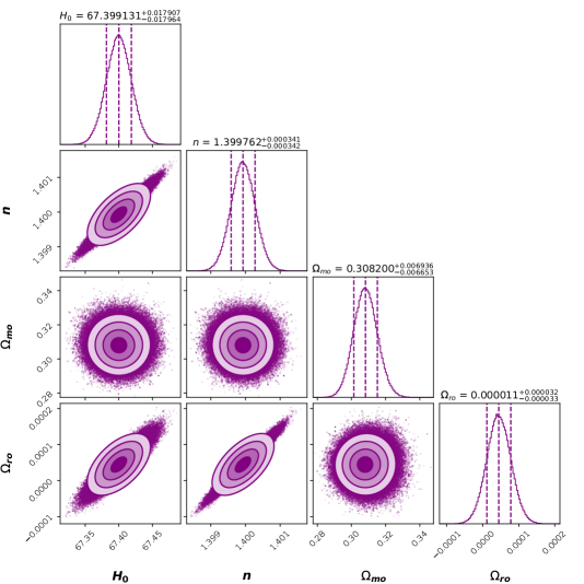
Figure 1: Likelihood contours plot for the model parameter $n$ of the power-law model along with cosmological parameters $H_{0}$, $\Omega_{m0}$ and $\Omega_{r0}$.

As shown in Fig. 1, from this analysis we have obtained most likely values of the Hubble constant $H_{0}$, matter density parameter $\Omega_{m0}$, radiation density parameter $\Omega_{r0}$ and the power-law model parameter $n$ respectively as $H_{0}=67.399131^{+0.017907}_{-0.017964}$, $\Omega_{m0}=0.303626^{+0.006936}_{-0.006653}$, $\Omega_{r0}=0.000011^{+0.000032}_{-0.000033}$ and $n=1.399762^{+0.000341}_{-0.000342}$. It is seen that the most likely value of $n$ is very close to $1.4$ and hence we will use it in the rest of our analysis.

The relation of cosmological evolution time $t$ and redshift $z$ for the power-law model can be obtained by substituting Eq. (11) for $H(z)$ in Eq. (7) as given by

$$\bigg{|}\frac{dt}{dz}\bigg{|}=(1+z)^{-1}\left[-\,\frac{2nR_{0}}{3(3-n)^{2}\Omega_{m0}}\Bigl{\{}(n-3)\Omega_{m0}(1+z)^{\frac{3}{n}}+2(n-2)\Omega_{r0}(1+z)^{\frac{n+3}{n}}\Bigl{\}}\right]^{-\,\frac{1}{2}}\!\!.$$ (12)

In Fig. 2, we have plotted the differential variation of cosmological time $t$ with respect to redshift $z$ i.e. the variation of $dt/dz$ with the redshift $z$ for different values for model parameter $n$ along with the that for the $\Lambda$CDM model.

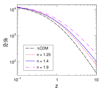
Figure 2: Variation of $dt/dz$ with the redshift $z$ for different values for the model parameter $n=1.25,1.4$ and $1.9$ along with the variation of the same for the $\Lambda$CDM model.

It is seen from Fig. 2 that the difference of variation of $dt/dz$ for the power-law and the $\Lambda$CDM model is very less significant for smaller values of $z\leq 0.2$, while that for higher value of $z$ it has shown a notable variation. Therefore for the rest of the paper, a possible higher value of redshift will have to be taken into account. Moreover, it should be mentioned that although $n=1.4$ is found as most suitable value of the parameter of the power-law model, we used other two values of $n$ in this plot to see how the model prediction varies from that of the $\Lambda$CDM model with different values of $n$. It is clear that the higher values of $n$ obviously show more deviation from the $\Lambda$CDM model prediction for all appropriate values of $z$ and hence the most favorable value $n=1.4$ shows appreciable behavior in this regard.

Table 1: Currently available observational Hubble parameter data $H^{obs}(z)$ [km s^-1 Mpc^-1]

$z$	$H^{obs}(z)$	Reference	$z$	$H^{obs}(z)$	Reference
0.0708	$69.0\pm 19.68$	[70]	0.48	$97.0\pm 62.0$	[78]
0.09	$69.0\pm 12.0$	[71]	0.51	$90.8\pm 1.9$	[75]
0.12	$68.6\pm 26.2$	[70]	0.57	$92.4\pm 4.5$	[79]
0.17	$83.0\pm 8.0$	[71]	0.593	$104.0\pm 13.0$	[72]
0.179	$75.0\pm 4.0$	[72]	0.60	$87.9\pm 6.1$	[77]
0.199	$75.0\pm 5.0$	[72]	0.61	$97.8\pm 2.1$	[75]
0.2	$72.9\pm 29.6$	[70]	0.68	$92.0\pm 8.0$	[72]
0.24	$79.69\pm 2.65$	[73]	0.73	$97.3\pm 7.0$	[77]
0.27	$77.0\pm 14.0$	[71]	0.781	$105.0\pm 12.0$	[72]
0.28	$88.8\pm 36.6$	[70]	0.875	$125.0\pm 17.0$	[72]
0.35	$84.4\pm 7.0$	[74]	0.88	$90.0\pm 40.0$	[78]
0.352	$83.0\pm 14.0$	[72]	0.9	$117.0\pm 23.0$	[71]
0.38	$81.9\pm 1.9$	[75]	1.037	$154.0\pm 20.0$	[72]
0.3802	$83.0\pm 13.5$	[76]	1.3	$168.0\pm 17.0$	[71]
0.40	$95.0\pm 17.0$	[71]	1.363	$160.0\pm 33.6$	[80]
0.4004	$77.0\pm 10.2$	[76]	1.43	$177.0\pm 18.0$	[71]
0.4247	$87.1\pm 11.2$	[76]	1.53	$140.0\pm 14.0$	[71]
0.43	$86.45\pm 3.68$	[73]	1.75	$202.0\pm 40.0$	[71]
0.44	$82.6\pm 7.8$	[77]	1.965	$186.5\pm 50.4$	[80]
0.4497	$92.8\pm 12.9$	[76]	2.34	$223.0\pm 7.0$	[81]
0.47	$89.0\pm 50.0$	[78]	2.36	$227.0\pm 8.0$	[82]
0.4783	$80.9\pm 9.0$	[76]

IV.2 Starobinsky Model and cosmological equations

The Starobinsky model of $f(R)$ gravity considered here is of the form [67]:

$$f(R)=\alpha R+\beta R^{2},$$ (13)

where $\alpha$ and $\beta$ are two free model parameters which are to be constrained by using observational data associated with a particular problem of study. Similar to the previous case the expression of the Hubble parameter $H(z)$ for the Starobinsky model can be obtained from Eq. (5) along with Eq. (7) as

$$H(z)=H_{0}\left[\frac{3\,\Omega_{m0}(1+z)^{3}+6\,\Omega_{r0}(1+z)^{4}+\left(\alpha R+\beta R^{2}\right)\!H_{0}^{-2}}{6(\alpha+2\beta R)\Bigl{\{}1-\frac{9\,\beta H_{0}^{2}\,\Omega_{m0}(1+z)^{3}}{\alpha(\alpha+2\beta R)}\Bigl{\}}^{2}}\right]^{\frac{1}{2}}.$$ (14)

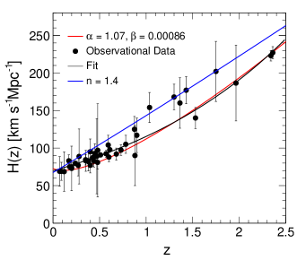
Figure 3: Least square fitting to the observational Hubble data set shown in Table 1 and the best fitted curve for the model parameters values $\alpha=1.07$ and $\beta=0.00086$. Also a fit to the power-law model for the model parameter $n=1.4$ is shown here.

To use this expression of $H(z)$ for further study we have to constraint the values of the model parameters $\alpha$ and $\beta$ within their realistic values as the behaviour of $H(z)$ depends significantly on these two model parameters. For this we have used the currently available observational Hubble parameter ($H^{obs}(z)$) data set [68] as shown in Table 1.

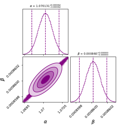
Figure 4: Likelihood contours plot for the $f(R)$ gravity Starobinsky model parameters $\alpha$ and $\beta$.

Here we have taken into account the combination of 43 observational Hubble parameter data against 43 distinct values of redshift in order to obtain the precise values of the aforementioned free model parameters, which should be consistent with the $\Lambda$CDM model at least around the current epoch i.e. $z=0$.

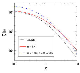
Figure 5: Variation of $dt/dz$ with respect to the redshift $z$ for the both $f(R)$ gravity power-law model and the Starobinsky model.

Using the least square fitting technique in ROOT software [69], we have plotted the best fitted curve to this set of Hubble parameter data with respect to the redshift as shown in Fig 3. From this best fitted curve we have inferred values of $\alpha$ and $\beta$ as $1.07$ and $0.00086$ respectively. Further, like the power-law model, we have plotted a corner plot for the Starobinsky model as well for the model parameters $\alpha$ and $\beta$, which is shown in Fig. 4. Here also we get the model parameter as $\alpha=1.070131^{+0.000062}_{-0.000062}$ and $\beta=0.000860$.

Now, we are in a position to write the expression for $dt/dz$ for this model and it can be expressed as

$$\bigg{|}\frac{dt}{dz}\bigg{|}=\big{[}(1+z)H_{0}\big{]}^{-1}\left[\frac{3\,\Omega_{m0}(1+z)^{3}+6\,\Omega_{r0}(1+z)^{4}+\frac{\alpha R+\beta R^{2}}{H_{0}^{2}}}{6(\alpha+2\beta R)\Bigl{\{}1-\frac{9\beta H_{0}^{2}\Omega_{m0}(1+z)^{3}}{\alpha(\alpha+2\beta R)}\Bigl{\}}^{2}}\right]^{-\frac{1}{2}},$$ (15)

In Fig.5, the variation of $dt/dz$ with the redshift $z$ is shown for the both $f(R)$ gravity power-law model and the Starobinsky model in the comparison with the prediction of the $\Lambda$CDM model. It can be observed that the power-law model shows very close behaviour with the $\Lambda$CDM for very small values of $z$, but their difference continuously increases with the increasing values of $z$ as mentioned already. Whereas the Starobinsky model shows consistently higher deviation from the $\Lambda$CDM model although there is gradually a slight inclination towards the $\Lambda$CDM model for higher $z$ values. Moreover, the Starobinsky model gives higher values of $dt/dz$ till $z\sim 3$ and after this value of $z$ the values of $dt/dz$ for the Starobinsky model decreases continuously with increasing $z$ in comparison to that of the power-law model. Further, both $f(R)$ gravity models show consistently higher $dt/dz$ values than that of the $\Lambda$CDM model depending on the values of $z$ within the range of our interest.

In the next section, we will employ the power law model and the Starobinsky model to calculate the cosmic ray density and differential flux using the results of this section.

V Cosmic ray density and flux in the domain of $f(R)$ gravity

The first thing that piques our curiosity is how the density of CRs is being modulated at a certain distance from the originating source in a TMF. For this it is necessary to calculate the density enhancement of CRs at a certain distance $r_{s}$ from the originating source while being surrounded by a TBF. We specifically wish to investigate its reliance on the energy of particles and take into account the transition from the diffusive propagation.

In the diffusive regime, the diffusion equation for the UHE particles propagating in an expanding Universe from a source which is located at a position ${\bf x}_{s}$ can be expressed as [23]

$$\frac{\partial n}{\partial t}+3H(t)\,n-b(E,t)\frac{\partial n}{\partial E}-n\,\frac{\partial n}{\partial E}-\frac{D(E,t)}{a^{2}(t)}\,\nabla^{2}n=\frac{Q_{s}(E,t)}{a^{3}(t)}\,\delta^{3}({\bf x}-{\bf{x}_{s}}),$$ (16)

where $H(t)=\dot{a}(t)/a(t)$ is the Hubble parameter as a function of cosmological time $t$, $\dot{a}(t)$ is time derivative of the scale factor $a(t)$, ${\bf x}$ denotes the comoving coordinates, $n$ is the density of particle at time $t$ and position ${\bf x}$, $Q_{s}(E)$ is the source function that depicts the number of emitted particles with energy $E$ per unit time. Thus, at time $t$, which corresponds to redshift $z$, $r_{s}={\bf x}-{\bf{x}_{s}}$. The energy losses due to the expansion of the Universe and interaction with CMB are described by

$$\frac{dE}{dt}=-\,b(E,t),\;\;b(E,t)=H(t)E+b_{int}(E).$$ (17)

Here $H(t)E$ represents the adiabatic energy losses due to expansion and $b_{int}(E)$ denotes the interaction energy losses. The interaction energy losses with CMB includes energy losses due to pair production and photopion production (for details see [2]). The general solution of Eq. (16) was obtained in [23] considering the particles as protons and it is given as

$$n(E,r_{s})=\int_{0}^{z_{i}}dz\,\bigg{|}\frac{dt}{dz}\bigg{|}\,Q(E_{g},z)\,\frac{\textrm{exp}\left[-r_{s}^{2}/4\lambda^{2}\right]}{(4\pi\lambda^{2})^{3/2}}\,\frac{dE_{g}}{dE},$$ (18)

where $z_{i}$ is the redshift of initial time when a particle was just emitted by source and $E_{g}$ is the generation energy at redshift $z$ of a particle whose energy is $E$ at $z=0$, i.e. at present time. The source function $Q(E_{g},z)$ is considered to follow a power-law spectrum $Q\varpropto E_{g}^{-\gamma_{g}}$ with $\gamma_{g}$ as the spectral index of generation at the source. $\lambda$ is the Syrovatsky variable [83, 17] and is given by

$$\lambda^{2}(E,z)=\int_{0}^{z}dz\,\bigg{|}\frac{dt}{dz}\bigg{|}\,(1+z)^{2}D(E_{g},z).$$ (19)

Here $\lambda(E,z)$ refers to the usual distance that CRs travel from the location of their production at redshift $z$ with energy $E_{g}$, to the present time at which they are degraded to energy $E$. The expression of the rate of dregadation of the energy at source of particles with respect to their energy at $z=0$, i.e. $dE_{g}/dE$ is given by [23]

$$\frac{dE_{g}}{dE}=(1+z)\ \textrm{exp}\left[\int_{0}^{z}dz\,\bigg{|}\frac{dt}{dz}\bigg{|}\left(\frac{\partial\,b_{int}}{\partial E}\right)\right].$$ (20)

It is clear that using Eqs. (12) and (15) in Eqs. (19) and (20) the density of UHE protons in the diffusive medium at any cosmological time $t$ with energy $E$ and at a distance $r_{s}$ from the source as given by Eq. (18) can be obtained as predicted by the $f(R)$ gravity power-law model and Starobinsky model respectively. So, in the following we will implement the power-law and Starobinsky model results from section IV to obtain the CR’s protons density enhancement factor, and subsequently the CR’s protons flux and energy spectrum as predicted by these two $f(R)$ gravity models.

V.1 Projections of $f(R)$ power-law model

To calculate the CR protons’ density (18) and hence its enhancement factor in the TMF of extragalactic space projected by the power-law model of $f(R)$ gravity, as a prerequisite we calculate first the Syrovatsky variable $\lambda$ for this model from Eq. (19) using Eq. (12) with different values of the model parameters $n$ and taking the feasible field parameter values as $l_{c}=0.1$ Mpc, $B=50$ nG and the corresponding critical energy of proton as $E_{c}=4.5$ EeV, and then study the behaviour of the variable $\lambda$ for the both Kolmogorov spectrum and Kraichnan spectrum. We also calculate this variable for the $\Lambda$CDM model for both the spectra for the comparison. In these calculations and rest ones we use the values of $z=0-5$ keeping in view of possible source locations of CRs as well as the present and probable future cosmological observable range.

       

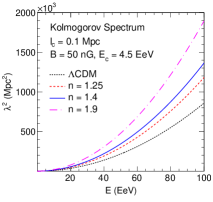
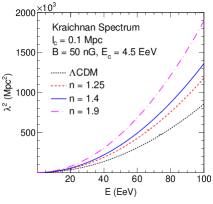
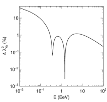
Figure 6: Variations of $\lambda^{2}$ with respect to energy $E$ for the Kolmogorov spectrum (left panel) and Kraichnan spectrum (middle panel) according to the $f(R)$ gravity power-law model and the standard $\Lambda$CDM model obtained by considering $l_{c}=0.1$ Mpc, $B=50$ nG and $E_{c}=4.5$ EeV. Right panel shows the percentage difference between $\lambda^{2}$ values for the Kolmogorov and Kraichnan spectra per average bin values of it for each energy bin of both the spectra for the power-law model with $n=1.4$. Here and rest of the corresponding calculations we use $z=0-5$.

The results of these calculations are shown in Fig. 6 with respect to energy $E$ for the Kolmogorov spectrum ($m=5/3$, $a_{L}\approx 0.23$ and $a_{I}\approx 0.9$) (left panel) and the Kraichnan spectrum ($m=3/2$, $a_{L}\approx 0.42$ and $a_{I}\approx 0.65$) (middle panel). It is seen from the figure that the value of $\lambda^{2}$ increases with increasing energy of the particle. The power-law model predicts higher $\lambda^{2}$ values for all values of $n$ in comparison to that of the $\Lambda$CDM models for both the spectra and this difference increases substantially with the increasing energy $E$. Similarly higher values of the parameter $n$ give increasingly higher values $\lambda^{2}$ in comparison to the smaller values of $n$. Apparently no difference can be observed between the values of $\lambda^{2}$ obtained for the Kolmogorov spectrum and the Kraichnan spectrum from the respective plots. So, to quantify the difference of values of $\lambda^{2}$ for these two spectra to a visible one we calculate the percentage difference between $\lambda^{2}$ values obtained for the Kolmogorov spectrum and Kraichnan spectrum per average bin values of $\lambda^{2}$ for each energy bin of both the spectra ($\Delta\lambda_{kk}^{2}(\%)$) for the power-law model with $n=1.4$, which is shown in the right panel of the figure. A peculiar behaviour of the variation of $\Delta\lambda_{kk}^{2}(\%)$ with energy is seen from the plot. The $\Delta\lambda_{kk}^{2}(\%)$ is energy dependent, it decreases rapidly with $E$ upto $\sim 0.4$ EeV, after which it shows oscillatory behaviour with the lowest minimum at $\sim 1.55$ EeV. At energies above $0.1$ EeV the values of $\Delta\lambda_{kk}^{2}(\%)$ are seen to be mostly below the $1\%$. Thus at these ultra high energies differences of $\lambda^{2}$ values for the Kolmogorov spectrum and the Kraichnan spectrum are not so significant.

In the diffusive regime the density of the particles has been enhanced by a factor depending on the energy, distance of the particles from the source and TMF properties. The density enhancement factor can be defined as the ratio of actual density to the density of particles that would lead for their rectilinear propagation, which is given by [3]

$$\xi(E,r_{s})=\frac{4\pi r_{s}^{2}c\,n(E,r_{s})}{\mathcal{L}(E)}$$ (21)

where $\mathcal{L}(E)$ is the spectral emissivity of the source, which has power-law dependency on the energy of the particles.

     

     

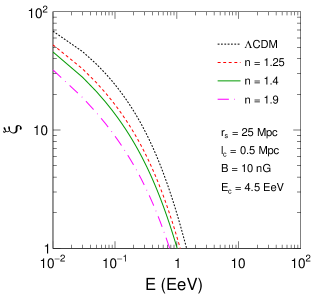
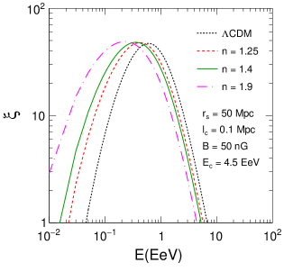
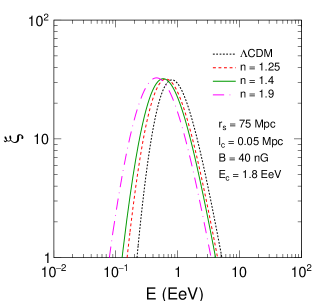
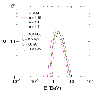
Figure 7: Variation of density enhancement factor $\xi$ with energy $E$ for the $f(R)$ gravity power-law model and the $\Lambda$CDM model obtained by considering $r=25-100$ Mpc, $l_{c}=0.025-0.5$ Mpc, $B=10-80$ nG and $E_{c}=1.8-4.5$ EeV.

The results of the enhancement of the density for a proton source and various parameter values obtained by numerically integrating Eq. (18), are displayed in Fig. 7. The distance to the source $r_{s}$, the magnetic field amplitude $B$, and its coherence length $l_{c}$ are the major factors that determine the lower-energy suppression of the density enhancement factor. For $r_{s}=25$ Mpc, $l_{c}=0.5$ Mpc, $B=10$ nG and $E_{c}=4.5$ EeV (upper left panel), the enhancement has become noticable for different gravity models in in the energy range $E<1$ EeV. For the energy range $0.01<E<10$ EeV, $r_{s}=50$ Mpc, $l_{c}=0.1$ Mpc, $B=50$ nG and $E_{c}=4.5$ EeV (upper right panel) are taken into account. In this case, below $1$ EeV the variation of enhancement for different gravity models is more distinguished compared to $E>1$ EeV. In the lower left panel, $r=75$ Mpc, $l_{c}=0.05$ Mpc, $B=40$ nG and $E_{c}=1.8$ EeV are used to plot the enhancement factor for the $\Lambda$CDM and $f(R)$ power-law models, while this is done for $r=100$ Mpc, $l_{c}=0.025$ Mpc, $B=80$ nG and $E_{c}=1.8$ EeV in the lower right panel. In the lower panels, the enhancement energy range is less as compared to the upper panels, which is lowest in the case of the lower right panel. As the distance from the source is far away, the enhancement of density is limited in a smaller range of energies, but shifted towards the higher energy side. The final verdict from the Fig.7 is that as the distance from the source $r_{s}$ increases, the enhancement becomes gradually model independent. Also one can appreciate that the $f(R)$ gravity power-law has done a perfect job by enhancing density in a wider range of energies as compared to the $\Lambda$CDM model.

     

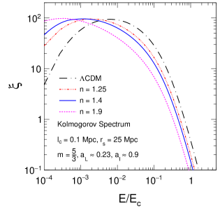
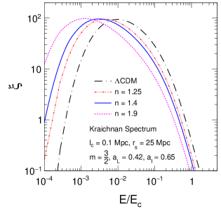
Figure 8: Variation of density enhancement $\xi$ with $\frac{E}{E_{c}}$. The left panel is for the Kolmogorov spectrum while the right panel is for the Kraichnan spectrum obtained by considering the $\Lambda$CDM and $f(R)$ gravity power-law models with $l_{c}=0.1$ Mpc and $r_{s}=25$ Mpc.

For a given source distance of $25$ Mpc and coherence length of $0.1$ Mpc, we depict the enhancement factor $\xi$ as a function of $E/E_{c}$ in Fig. 8 to better highlight the fact that for $E/E_{c}<0.01$ the Kolmogorov spectrum (left panel) and Kraichnan spectrum (right panel) have shown different behaviours while for $E/E_{c}>0.01$ the both Kolmogorov and Kraichnan spectra have shown similar patterns. In this case, the $f(R)$ power-law model is more suitable as it gives the enhancement in the higher as well as lower values of $E/E_{c}$, while in the case of the $\Lambda$CDM the range it gives the enhancement is less wider than the power-law model. From this Fig. 8 it is clearly seen that the kolmogorov spectrum has given a better range of $E/E_{c}$ than Kraichnan spectrum for the both $\Lambda$CDM and $f(R)$ power-law model.

     

     

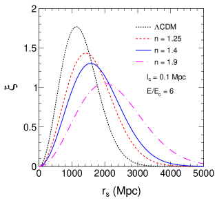
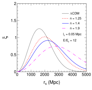
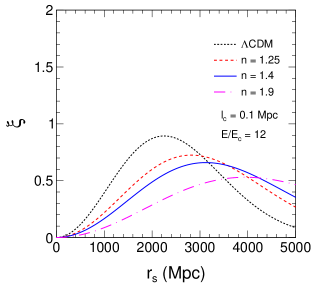
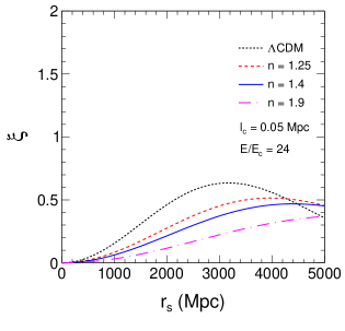
Figure 9: Variation of $\xi$ with source distance $r_{s}$ for the $\Lambda$CDM model and $f(R)$ power-law model obtained by considering $l_{c}=0.1$ (upper and lower left panel), $l_{c}=0.05$ (upper and lower right panel)and $E/E_{c}=6$ (upper left panel), $E/E_{c}=12$ (lower left and upper right panel), $E/E_{c}=24$ (lower right panel).

The diffusive character of propagation UHE protons is shown in Fig. 9. Here we plot the density enhancement $\xi$ as a function of source distance $r_{s}$. In this case, we fix the coherence length $l_{c}=0.1$ Mpc, while $E/E_{c}=6$ and $E/E_{c}=12$ in the upper left and the lower left panel respectively. From these two panels, we can say that the lower $E/E_{c}$ value results in a higher peak of the density enhancement with the peak position towards the smaller values of $r_{s}$. Again, the $\Lambda$CDM model shows the highest peak in the CRs density enhancement, while the $f(R)$ gravity power-law model depicts a better distribution of enhancement with the source distance. For the model parameters $n=1.25$ and $n=1.4$, it results in a similar distribution while for $n=1.9$, it shows a larger distribution. From the lower left panel and the upper right panel, it is clearly seen that the enhancement peak height and position depend on the coherence length $l_{c}$ also. For the higher value of $l_{c}$ the peak height decreases, but it shifts away from the source. In the lower right panel, we have considered a larger value of $E/E_{c}=24$ which results in a very poor peak in the both $\Lambda$CDM and the $f(R)$ power-law models. So from these results, we can finally say that for suitable values of $l_{c}$ and $E/E_{c}$, the $\Lambda$CDM model depicts a better peak, while $f(R)$ power-law model depicts the enhancement in a much wider distribution.

For reckoning the diffuse spectrum of UHE particles the separation between sources play a crucial role. If the sources are distributed uniformly with separations, which are very smaller than the propagation and the interaction lengths, then the diffuse spectrum of UHE particles has a universal form, regardless of the mode of propagation of such particles [27]. To this end the explicit form of the source function $Q(E,z)$ for the power-law generation of the particles can be written as [29]

$$Q(E,z)=\mathcal{L}_{0}(1+z)^{m}Kq_{gen}(E_{g}),$$ (22)

where $\mathcal{L}_{0}=\int\mathcal{L}(E)\,dE$ is the total emissivity, $(1+z)^{m}$ represents the probable cosmological evolution of the sources, $K$ is a normalisation constant with $K=\gamma_{g}-2$ for $\gamma_{g}>2$ and for $\gamma_{g}=2$, $K=(\ln E_{max}/E_{min})^{-1}$ and $q_{gen}=E^{-\gamma_{g}}_{g}$ (see Appendix A for $E_{g}$). Utilizing the formalisation of Refs. [13, 23], it is possible to determine the spectrum of UHE protons in the model with uniform source distribution and hence one can obtain the diffuse flux of UHE protons as

$$J_{p}(E)=\frac{c}{4\pi}\,\mathcal{L}_{0}K\int_{0}^{z_{max}}\!\!dz\,\biggl{|}\frac{dt}{dz}\biggl{|}\,(1+z)^{m}q_{gen}(E_{g})\,\frac{dE_{g}}{dE}.$$ (23)

Following Eq. (12) one can rewrite this diffuse flux Eq. (23) as

$$J_{p}(E)=\frac{c}{4\pi}\,\mathcal{L}_{0}K\displaystyle\int_{0}^{z_{max}}\!\!dz \bigg{[}(1+z)^{-1}\Big{[}-\frac{2\,nR_{0}}{3(3-n)^{2}\ \Omega_{m0}}\,\Bigl{\{}(n-3)\Omega_{m0}(1+z)^{\frac{3}{n}}$$

$$+2(n-2)\,\Omega_{r0}(1+z)^{\frac{n+3}{n}}\Bigl{\}}\Big{]}^{-\frac{1}{2}}\bigg{]}(1+z)^{m}q_{gen}(E_{g})\,\frac{dE_{g}}{dE}.$$ (24)

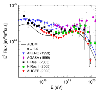
Figure 10: UHECR proton flux is shown for the $\Lambda$CDM model and the $f(R)$ gravity power-law model in comparison with various experimental data such as AKENO-AGASA [52, 53], HiRes [54] and AUGER [56] experiments.

The spectrum given by Eq. (23) is known as the universal spectrum as it is independent of the mode of propagation of particles which is the consequence of the small separation of sources as mentioned earlier. The shape of the universal spectrum may theoretically be changed by variety of effects, which include the fluctuations in interaction, discreteness in source distribution, large-scale inhomogeneous source distribution, local source overdensity or deficit, and discrete source distribution. However, the aforementioned effects only slightly change the form of the universal spectrum, with the exception of energies below $1$ EeV and above the GZK cutoff. Numerical simulations demonstrate that the energy spectrum is changed by the propagation of UHE protons in the strong magnetic fields depending on the separation of sources. For small separation of sources with their uniform distribution the spectrum becomes the universal one as mentioned already [84, 85]. In Fig. 10, we plot the diffusive flux with no cosmological evolution ($m=0$) [29, 27]. The emissivity $\mathcal{L}_{0}$ is taken to fit the curve with the available observational data [29]. It is clear that the $f(R)$ gravity power-law model curve with $n=1.4$ has satisfied the majority of AKENO, AGASA and HiRes I data, while the $\Lambda$CDM model satisfies AUGER and HiRes II. Moreover, the $f(R)$ gravity power-law model curve passes through within the error range of most of the experimental data for the whole UHECRs range. Further, throughout this energy range $f(R)$ gravity power-law model gives higher proton flux than that of the $\Lambda$CDM model. A dip is seen at the energy range of $1-10$ EeV, while at about $30$ EeV a bump is observed.

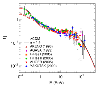
Figure 11: Spectra of modification factor with $\gamma_{g}=2.7$ in comparison with different experimental data such as AKENO-AGASA [52, 53], HiRes [54], YAKUTSK [57] and AUGER [55] for the $\Lambda$CDM and $f(R)$ gravity power-law model.

These two signatures, the dip and bump are also observed in the modification factor of the energy spectrum plot as shown in Fig. 11. The modification factor of the energy spectrum is a convenient parameter for doing the analysis of the energy spectrum of UHECRs. This parameter corresponds to the enhencement factor of density of UHECR particles discussed earlier. The modification factor of energy spectrum $\eta(E)$ is calculated as the ratio of the universal spectrum $J_{p}(E)$ after accounting for all energy losses to the unmodified spectrum $J_{p}^{unm}(E)$, in which only adiabatic energy losses due to the red shift are taken into consideration [29], i.e.

$$\eta(E)=\frac{J_{p}(E)}{J_{p}^{unm}(E)}$$ (25)

Without any cosmological evolution the unmodified spectrum can be written as

$$J_{p}^{unm}(E)=\frac{c}{4\pi}\,\mathcal{L}_{0}(\gamma_{g}-2)E^{-\gamma_{g}}\int_{0}^{z_{max}}\!\!dz\,\biggl{|}\,\frac{dt}{dz}\biggl{|}(1+z)^{(1-\gamma_{g})}.$$ (26)

The modification factor as a function of energy for the spectral index $\gamma_{g}=2.7$ is shown in Fig. 11 for the $f(R)$ gravity power-law model and the $\Lambda$CDM model. At about $1$ EeV, a dip is seen in the spectrum as predicted by both the models in agreement with the observation of AKENO, HiRes II and YAKUTSK arrays. Also a good agreement with AGASA, HiRes I and AUGER data for the bump in the spectrum is seen. One can observe that for energy $E<1$ EeV, the modification factor becomes higher. The modification factor $\eta>1$ depicts the presence of other components of CRs which are of mainly galactic origin. From Fig. 11, it can also be said that the modification factor of the energy spectrum is less model dependent parameter.

V.2 Projections of Starobinsky $f(R)$ gravity model

For this model of $f(R)$ gravity also we will follow the same procedure as we have already done in the case of the power-law model. So here also we have to calculate the Syrovatsky variable $\lambda^{2}$ and for this purpose we express $\lambda^{2}(E,z)$ from Eq. (19) using Eq. (15) for the Starobinsky model as

$$\lambda^{2}(E,z)=H_{0}^{-1}\int_{0}^{z}dz\,(1+z)\left[\frac{3\,\Omega_{m0}(1+z)^{3}+6\,\Omega_{r0}(1+z)^{4}+\frac{\alpha R+\beta R^{2}}{H_{0}^{2}}}{6(\alpha+2\beta R)\Bigl{\{}1-\frac{9\beta H_{0}^{2}\Omega_{m0}(1+z)^{3}}{\alpha(\alpha+2\beta R)}\Bigl{\}}^{2}}\right]^{-\frac{1}{2}}\!\!\!\!\!\!\!D(E_{g},z).$$ (27)

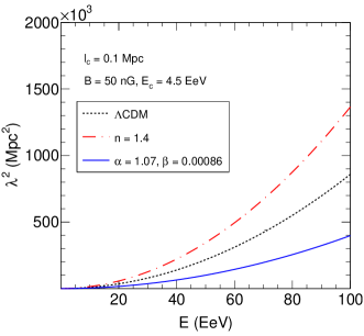
Figure 12: Variation of $\lambda^{2}$ with energy $E$ for the $\Lambda$CDM, $f(R)$ gravity power-law and Starobinsky models by considering $r_{s}=50$ Mpc, $l_{c}=0.1$ Mpc, $B=50$ nG and $E_{c}=4.5$ EeV.

In Fig. 12 we plot the variation of $\lambda^{2}$ with respect to energy for the $f(R)$ gravity Starobinsky model and power-law model in comparison with the $\Lambda$CDM model. For this we consider the source distance $r_{s}=50$ Mpc, the coherence length $l_{c}=0.1$ Mpc and the strength of the TMF, $B=50$ nG, and use only the Kolmogorov spectrum of the diffusion coefficient. A noticeable variation with respect to the energy is observed in $\lambda^{2}$ values for all of the mentioned gravity models. Moreover, the $f(R)$ gravity Starobinsky model gives the lowest value of $\lambda^{2}$ although its pattern of variation with respect to energy is similar for all the three models.

     

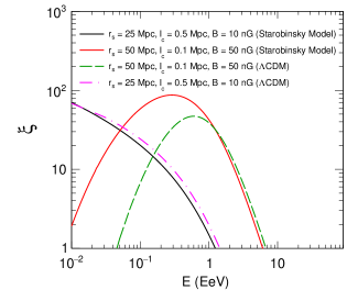
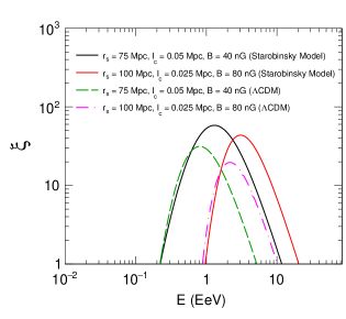
Figure 13: Variation of density enhancement $\xi$ with respect to energy $E$ for the $f(R)$ gravity Starobinsky model in comparison with the $\Lambda$CDM model obtained by using different sets of parameter as $r=25-100$ Mpc, $l_{c}=0.025-0.5$ Mpc, $B=10-80$ nG and $E_{c}=1.8-4.5$ EeV.

Similarly, using Eqs. (18), (20) and (27) in Eq. (21) we calculate the UHE particle density enhancement factor $\xi(E,r_{s})$ for the Starobinsky model. The expression for $\xi(E,r_{s})$ for this model can be wrriten as

$$\xi(E,r_{s})=4\pi r_{s}^{2}H_{0}^{-1}\!\int_{0}^{z_{i}}\!\!dz\,(1+z)^{-1}\!\left[\frac{3\,\Omega_{m0}(1+z)^{3}+6\,\Omega_{r0}(1+z)^{4}+\frac{\alpha R+\beta R^{2}}{H_{0}^{2}}}{6(\alpha+2\beta R)\Bigl{\{}1-\frac{9\beta H_{0}^{2}\Omega_{m0}(1+z)^{3}}{\alpha(\alpha+2\beta R)}\Bigl{\}}^{2}}\right]^{-\frac{1}{2}}\!\!\!\!\!\frac{\textrm{exp}[-r_{s}^{2}/4\lambda^{2}]}{(4\pi\lambda^{2})^{3/2}}\,\frac{dE_{g}}{dE}.$$ (28)

Considering the source distances $r_{s}=25$ Mpc and $50$ Mpc, coherence lengths $l_{c}=0.5$ Mpc and $0.1$ Mpc, and field strengths $B=10$ nG and $50$ nG, we plot the density enhancement factors as a function of energy $E$ for both the Starobinsky model and $\Lambda$CDM model in the left panel of Fig. 13 and that for $r_{s}=75$ Mpc and $100$ Mpc, $l_{c}=0.025$ Mpc and $0.05$ Mpc, and $B=40$ nG and $80$ nG in the right panel of Fig. 13. Note that in the figure, we constrain the critical energy i.e., $E_{c}=4.5$ EeV and $E_{c}=1.8$ EeV for the left and the right panel respectively. One can see that the enhancement of density precisely relies on the parameters we consider and for the different parameters we find a very dintinct result in each of the cases. The distinction between enhancement factors for the Starobinsky model and $\Lambda$CDM model is clearly visible. The Starobinsky model gives a higher peak and wider range of the enhancement factor than that given by the $\Lambda$CDM model. Moreover, for smaller to medium values of $r_{s}$ the difference between two models on the higher energy side is very small, while for higher values of $r_{s}$ the it is very small on the lower energy side of the enhancement factor plots.

     

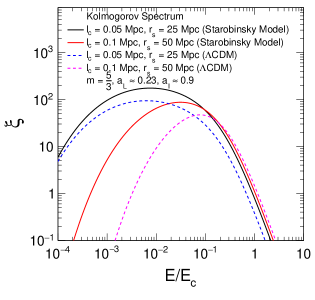
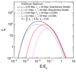
Figure 14: Variation of density enhancement $\xi$ with $\frac{E}{E_{c}}$ for the Starobinsky model in comparison with the $\Lambda$CDM model. The left panel is for the Kolmogorov spectrum while the right panel is for the Kraichnan spectrum obtained by considering different sets of coherence length $l_{c}$ and source distance $r_{s}$.

For more distinct observation of the density enhancement features, we plot the density enhancement as a function of $E/E_{c}$ in Fig. 14 for the Starobinsky model as well as for the $\Lambda$CDM model. Using $l_{c}=0.05$ Mpc, $r_{s}=25$ Mpc (solid line) and $l_{c}=0.1$ Mpc, $r_{s}=50$ Mpc (dotted line), a Kolmogorov spectrum is shown in the left panel for both the models. A remarkable variation is observed for $E/E_{c}<0.1$ in both the sets of values, although for $E/E_{c}>0.1$ a quite similar results we have obtained. Using the same sets of parameters, a Kraichnan spectrum is also plotted in the right panel of Fig.14. The peaks of the both spectrum are almost in the same energy range but the variation in lower $E/E_{c}$ is quite different.

     

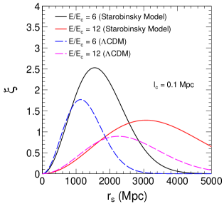
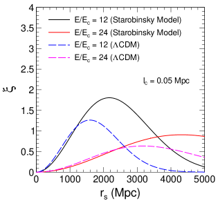
Figure 15: Variation of $\xi$ with source distance $r_{s}$ obtained by considering the parameter as $l_{c}=0.1$, $\frac{E}{E_{c}}=6,12$ (left panel) and $l_{c}=0.05$, $\frac{E}{E_{c}}=12,24$ (right panel) for both the Starobinsky model and the $\Lambda$CDM model.

Similar to the case of $f(R)$ gravity power-law model, here also we plot the density enhancement factor $\xi$ with respect to the source distance $r_{s}$ by keeping fixed the coherence length $l_{c}=0.1$ Mpc for $E/E_{c}=6$ (black line) and $12$ (red line) in the left panel of Fig. 15 and that same for $l_{c}=0.05$ Mpc with $E/E_{c}=12$ (black line) and $24$ (red line) in the right panel of this figure to understand the propagation of UHECR protons in the light of the Starobinsky model in comparison with the $\Lambda$CDM model. From this figure, one can see that similar to the power-law model the peak of the enhancement is higher for smaller values of $E/E_{c}$, whereas the range of the distribution of the enhancement is wider for smaller values of $l_{c}$.

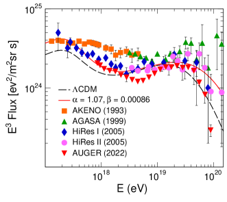
Figure 16: UHECR protons flux is shown for the $f(R)$ gravity Starobinsky model and compare with various experimental data such as AKENO-AGASA [52, 53], HiRes [54] and AUGER [56] along with the flux for the $\Lambda$CDM model.

The diffuse UHECR proton flux for the $f(R)$ gravity Starobinsky model can be expressed as

$$J_{p}(E)=\frac{c\,H_{0}}{4\pi}\,\mathcal{L}_{0}K\!\int_{0}^{z_{max}}\!\!\!\!dz\,(1+z)^{m-1}\left[\frac{3\,\Omega_{m0}(1+z)^{3}+6\,\Omega_{r0}(1+z)^{4}+\frac{\alpha R+\beta R^{2}}{H_{0}^{2}}}{6(\alpha+2\beta R)\Bigl{\{}1-\frac{9\beta H_{0}^{2}\Omega_{m0}(1+z)^{3}}{\alpha(\alpha+2\beta R)}\Bigl{\}}^{2}}\right]^{-\frac{1}{2}}\!\!\!\!\!\!q_{gen}(E_{g})\,\frac{dE_{g}}{dE}.$$ (29)

In Fig. 16, we plot this flux (29) as a function of energy by considering the Starobinsky model parameters as we have discussed in section IV. From the figure, we can see that the Starobinsky model’s spectrum has a very good agreement with AUGER data within the energy range $\sim 0.8-1.1$ EeV depicting the dip and bump. In the low energy range, the AKENO and HiRes I, and in the higher energy range both HiRes II and AUGER give a reasonably good agreement with the Starobinsky model one. Similar to the $f(R)$ gravity power-law model the Starobinsky model also gives high flux in comparison to the $\Lambda$CDM model over the almost entire energy range considered. A detailed comparison of the diffuse fluxes for all the models considered in this work will be discussed in the next section.

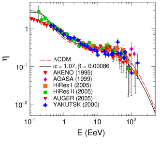
Figure 17: Spectra of modification factor for the $f(R)$ gravity Starobinsky model along with that for the $\Lambda$CDM model with $\gamma_{g}=2.7$, which are in comparison with different experimental data such as AKENO-AGASA [52, 53], HiRes [54], YAKUTSK [57] and AUGER [55] experiments.

Finally, for the calculation of the modification factor $\eta$ of the energy spectrum, the unmodified flux of UHECR protons for the Starobinsky model is given by

$$J_{p}^{unm}(E)=\frac{c\,H_{0}}{4\pi}\,\mathcal{L}_{0}(\gamma_{g}-2)E^{-\gamma_{g}}\int_{0}^{z_{max}}\!\!\!dz\,(1+z)^{-\gamma_{g}}\left[\frac{3\,\Omega_{m0}(1+z)^{3}+6\,\Omega_{r0}(1+z)^{4}+\frac{\alpha R+\beta R^{2}}{H_{0}^{2}}}{6(\alpha+2\beta R)\Bigl{\{}1-\frac{9\beta H_{0}^{2}\Omega_{m0}(1+z)^{3}}{\alpha(\alpha+2\beta R)}\Bigl{\}}^{2}}\right]^{-\frac{1}{2}}\!\!\!\!\!\!.$$ (30)

Fig. 17 shows the behaviour of the modification factor for the Starobinsky model along with that of the $\Lambda$CDM model, which are compared with experimental data as in the previous cases. One can observe that for $E<0.9$ EeV the modification factor $\eta>1$, which signifies the presence of other components for the galactic origin of CRs like the $f(R)$ gravity power-law model. The observational data have given a good agreement with the calculated modification factor spectra with dip as well as bump for both the Starobinsky model and $\Lambda$CDM model. It is also clear that the modification factor is very weakly model dependent as seen in the case of the power-law model also.

VI Discussions and conclusions

The believable sources of UHECRs are of extragalatic in origin [2, 86]. Accordingly the propagation mechanisms of UHECRs through the extragalactic space is one of prime issues of study since the past several decades. It can be inferred that in the propagation of UHECRs across the extragalactic space, the TMFs that exist in such spaces and the current accelerated expansion of the Universe might play their crucial roles. Thus this idea led us to study the propagation of UHECRs in the TMFs in the extragalactic space in the light of $f(R)$ theory of gravity and to compare the final outcomes with the experimental data of various world class experiments on UHECRs. The $f(R)$ theory of gravity is the simplest and one of the successful MTGs that could explain the current accelerated expansion of the Universe. To this end, we have considered two $f(R)$ gravity models, viz., the power-law model and the Starobinsky models. The Starobinsky model of $f(R)$ gravity is the widely used most viable model of the theory [67, 66, 50]. Similarly the power-law model is also found to be suitable in various cosmological and astrophysical perspectives [66]. The basic cosmological equations for these two $f(R)$ gravity models, which are required for this study are taken from the Ref. [66]. Independent parameters of the models are first constrained by using the recent observational data. A corner plot along with the confidence level plot is used to further constraint the said model parameters as well. The relation between the redshift $z$ and the evolution time $t$ is calculated for both the models. The UHECRs density $n(E,r_{s})$ and hence the enhancement factor of the density $\xi(E,r_{s})$ are obtained and they are calculated numerically for both the models of $f(R)$ gravity.

Figure 18: Density enhancement factor $\xi$ as a function of source distance is shown for the power-law and the Starobinsky model of $f(R)$ gravity in comparison with that for the $\Lambda$CDM model by considering $l_{c}=0.1$ Mpc and $E/E_{c}=6$.

A comparative analysis has been performed between the predictions of the power-law model and Starobinsky model of $f(R)$ gravity along with the same of the $\Lambda$CDM model for the density enhancement factor $\xi$ as a function of source distance $r$ in Fig. 18. In this analysis we consider the coherence length $l_{c}=0.1$ Mpc and the fraction of energy and critical energy, $E/E_{c}=6$. One can observe that at $r<1000$ Mpc, the variation of $\xi$ for the Starobinsky model and the $\Lambda$CDM is not very different but at the far distance from the source, the behaviour of these two model is quite different in terms of the peak position of the enhancement and the range of the source distance where the enhancement takes place. In the case of the $f(R)$ power-law model, the enhancement is less than the Starobinsky model and the $\Lambda$CDM model, but it gives the density enhancement in a much wider range than the $\Lambda$CDM model. In fact it gives the same range of source distance distribution in the enhancement and gives the peak of enhancement at the same distance as that of the Starobinsky model although the enhancement is comparatively low. Another comparative analysis has been done in Fig. 19 (left panel) for the CRs density enhancement with energy. For this purpose we take the parameters as $r_{s}=50$ Mpc, $l_{c}=0.1$ Mpc, $B=50$ nG and $E_{c}=4.5$ EeV.

     

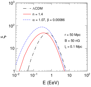
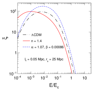
Figure 19: Density enhancement factor $\xi$ as a function of energy $E$ of UHECR protons obtained by considering $r_{s}=50$ Mpc, $l_{c}=0.1$ Mpc, $B=50$ nG and $E_{c}=4.5$ EeV (left panel), and also as a function of $E/E_{c}$ of the same particles for $r=25$ Mpc and $l_{c}=0.05$ Mpc (right panel). Both panels are shown for the power-law model, Starobinsky model and the $\Lambda$CDM model.

The Starobinsky model has given the best results as compared with other two models. From the left panel of Fig. 19, we see that at lower energies i.e., below $1$ Eev, the enhancement is different for different energy values including the peaks for the all three models. But if we take a look at the higher values of energy, the all three models depict almost similar results in the enhancement. One can say that the maximum value of enhancement for the power-law model and the $\Lambda$CDM model is approximately the same but the power-law model has covered a wider range of energy values than the $\Lambda$CDM model. While the Starobinsky model gives the highest enhancement value as well as the enhancement in a much wider range of energy values. The right panel of Fig. 19 is plotted to show the variation of density enhancement as a function of $E/E_{c}$. In this panel, we consider the coherence length $l_{c}=0.05$ Mpc and source distance $r_{s}=25$ Mpc to demonstrate the behaviour of enhancement with the per unit increase of energy with respect to the critical energy. It is seen that at $E/E_{c}=10^{-4}$, the value of enhancement for the Starobinsky model and $\Lambda$CDM is approximately same, while the $f(R)$ power-law model has shown a higher value of enhancement at this point. But as the fraction of energy is increased, the Starobinsky model has given a better result of enhancement as compared to the other two models.

     

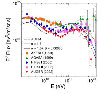
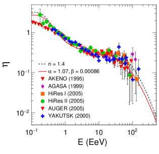
Figure 20: Calculated $E^{3}$ magnified spectra of UHECR protons for the $\Lambda$CDM model (black dotted line), the $f(R)$ gravity power-law model (blue line) and the Starobinsky model (red line) in comparison with the AKENO-AGASA [52, 53], HiRes [54] and AUGER [56] detectors’ data (left panel), and the modification factors of the same in comparison with the AKENO-AGASA [52, 53], HiRes [54], AUGER [55] and YAKUTSK [57] detectors’ data.

We calculate the $E^{3}$ magnified flux numerically for the both $f(R)$ gravity power-law and Starobinsky models and plot them along with that for the $\Lambda$CDM model in Fig. 20 (left panel). We also compare our calculations with the available observational data of AKENO-AGASA [52, 53], HiRes [54] and AUGER [56] detectors. In the low energy case, both the $f(R)$ models have shown very similar results, while at the higher energy a different result is obtained. All of these models have shown some agreement with the observational detectors’ data, but the $f(R)$ Starobinsky model has depicted a very good result in the lower as well as higher energy range for predicting dip and bump. Starting from AKENO as well as HiRes I data, it gives a good agreement with AUGER and HiRes II for the dip and bump respectively. For the power-law and $\Lambda$CDM models, the dip is found at around $3$ EeV while that for the Starobinsky model is at around $4$ EeV. The power-law model gives the higher flux than that of the Starobinsky model for the energy range around $0.2-30$ EeV and that of the $\Lambda$CDM model for the whole range of energy considered. Moreover, the power-law model favours the GZK cutoff more significantly than the Starobinsky model. The prediction of the Starobinsky model is matching very well with the $\Lambda$CDM model at around $10$ EeV energies, otherwise it shows higher flux than the $\Lambda$CDM model. Further, it is interesting note that the fluxes given by the both $f(R)$ gravity models lay well within the combined data range of all the UHECRs experiments considered here, whereas that of the $\Lambda$CDM model remains almost outside this range for the energies below $1.1$ EeV. Since the analysis of the bump and dip is more convenient in respect of the modification factor. We do not include in this analysis here the $\Lambda$CDM model because this factor is less model dependent and in the previous section we have already done the analysis with the $\Lambda$CDM model. From the right panel of Fig. 20, we see that in the lower energy range the origin of CRs appears to be of the galactic origin. We observe the dip in the spectrum at around $4$ EeV and it agrees with the observational data. Thus it can be concluded that the $f(R)$ gravity models considered here are found to be noteworthy with some limitations depending upon the range of energies in explaining the propagations of UHECRs and hence the observed data of their fluxes. Consequently, it is worth mentioning that by extending the work with these models it would be interesting to study the localised low scale anisotropies CRs that arise at their highest energies. So, we keep this as one of the future prospects of study.

Appendix A Parametric function for the generation energy $E_{g}$

For the complex nature of the dependence of the generation energy $E_{g}$ on the energy $E$ of UHECR particles, we considered a parametric function for the generation energy in this work as given by

$$F(c_{1},c_{2},c_{3},c_{4})\equiv c_{1}E+c_{2}E^{2}\exp{\left(-\frac{c_{3}}{E}\right)}+(1+c_{4}E)\exp{\left(-\frac{1}{E}\right)},$$

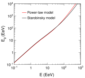
Figure 21: Variation of generation energy $E_{g}$ with respect to energy $E$ for the $f(R)$ gravity power-law model and Starobinsky model.

where $c_{1}$, $c_{2}$, $c_{3}$ and $c_{4}$ are constant parameters to be determined. In the function the first term represents the energy loss due to red-shift (expansion of the Universe), the second term the energy loss due to the pair production process with the CMB and the third term the photopion reaction with the CMB that dominates at higher energies [87]. For the $f(R)$ gravity power-law model we estimate the $E_{g}$ as

$$E_{g}\simeq F(1.2,0.035,-20,1.4),$$ (31)

and we estimate that for the Starobinsky model as

$$E_{g}\simeq F(1.47,0.02,-18.5,1.66).$$ (32)

In Fig. 21, a variation of $E_{g}$ with respect to $E$ is plotted for the power-law model and the Starobinsky model. For $E<1$ EeV, the variation is linear and above this energy $E_{g}$ is increasing non-linearly with the energy $E$. The difference between the estimated $E_{g}$’s by the power-law model and the Starobinsky model is noticeable at higher energies above $1$ EeV.

References

- [1] V. F. Hess, Uber Beobachtungen der durchdringenden Strahlung bei sieben Freiballonfahrten, Phys. Z. 13, 1084 (1912).
- [2] D. Harari, S. Mollerach, E. Roulet, Anisotropies of ultrahigh energy cosmic rays diffusing from extragalactic sources, Phys. Rev. D 89, 123001 (2014) [arXiv:1312.1366].
- [3] S. Mollerach, E. Roulet, Ultrahigh energy cosmic rays from a nearby extragalactic source in the diffusive regime, Phys. Rev. D 99, 103010 (2019) [arXiv:1903.05722].
- [4] V. Berezinsky, A. Z. Gazizov, O. Kalashev, Cascade photons as test of protons in UHECR, Astropart. Phys., 84, 52 (2016) [arXiv:1606.09293 ].
- [5] V. Berezinsky, A. Z. Gazizov, S. I. Grigorieva, Signatures of AGN model for UHECR [arXiv:astro-ph/0210095].
- [6] M. Nagano, A. A. Watson, Observations and implications of the ultrahigh-energy cosmic rays, Rev. Mod. Phys. 72, 689 (2000).
- [7] P. Bhattacharjee, G. Sigl, Origin and propagation of extremely high-energy cosmic rays, Phys. Rept. 327 (2000) [arXiv:astro-ph/9811011].
- [8] A. V. Olinto, Ultra High Energy Cosmic Rays: The theoretical challenge, Phys. Rept. 333 (2000) [arXiv:astro-ph/0002006].
- [9] S. Mollerach, E. Roulet, Anisotropies of ultrahigh-energy cosmic rays in a scenario with nearby sources, Phys. Rev. D 105 063001 (2022) [arXiv:2111.00560].
- [10] K. Greisen, End to the Cosmic-Ray Spectrum?, Phys. Rev. Lett. 16, 748 (1966).
- [11] G. T. Zatsepin, V. A. Kuzmin, Upper Limit of the Spectrum of Cosmic Rays, JETP. Lett. 4, 78 (1966).
- [12] C. T. Hill, D. N. Schramm, Ultrahigh-energy cosmic-ray spectrum, Phys. Rev. D 31, 564 (1985).
- [13] V. Berezinsky, S. I. Grigorieva, A bump in the ultra-high energy cosmic ray spectrum , Astron. Astroph. 199, 1 (1988)
- [14] S. Yoshida, M. Teshima, Energy Spectrum of Ultra-High Energy Cosmic Rays with Extra-Galactic Origin, Prog. Theor. Phys., 89, 833 (1993).
- [15] T. Stanev et al., Propagation of ultrahigh energy protons in the nearby universe, Phys. Rev. D 62, 093005 (2000) .
- [16] A. D. Supanitsky, Cosmic ray propagation in the Universe in presence of a random magnetic field, JCAP 04, 046 (2021) [arXiv:2007.09063].
- [17] S. Mollerach, E. Roulet, Magnetic diffusion effects on the Ultra-High Energy Cosmic Ray spectrum and composition, JCAP 10, 013 (2013) [arXiv:1305.6519].
- [18] D. Wittkowski for The Pierre Auger Collaboration, Reconstructed properties of the sources of UHECR and their dependence on the extragalactic magnetic field, PoS 563 (ICRC2017).
- [19] M. Unger, G. R. Farrar, L. A. Anchordoqui, Origin of the ankle in the ultra-high energy cosmic ray spectrum and of the extragalactic protons below it, Phys. Rev. D 92, 123001 (2015) [arXiv:1505.02153].
- [20] N. Globus, D. Allard, E. Parizot, A complete model of the CR spectrum and composition across the Galactic to Extragalactic transition, Phys. Rev. D 92, 021302 (2015) [arXiv:1505.01377].
- [21] R. A. batista et.al., CRPropa 3—a public astrophysical simulation framework for propagating extraterrestrial ultra-high energy particles, JCAP 05, 038 (2016) [arXiv:1603.07142].
- [22] O. E. Kalashev and E. Kido, Simulations of ultra-high-energy cosmic rays propagation, J. Exp. Theor. Phys. 120, 790 (2015) [arXiv:1406.0735].
- [23] V. Berezinsky, A. Z. Gazizov, Diffusion of Cosmic Rays in the Expanding Universe. I., Astrophys. J. 643, 8 (2006) [arXiv:astro-ph/0512090].
- [24] D. J. Bird et al., Detection of a Cosmic Ray with Measured Energy Well beyond the Expected Spectral Cutoff due to Cosmic Microwave Radiation, Astrophys. J. 441 (1995) [arXiv:astro-ph/9410067].
- [25] The High Resolution Fly’s Eye Collaboration, Monocular Measurement of the Spectrum of UHE Cosmic Rays by the FADC Detector of the HiRes Experiment, Astropart. Phys. 23, 157 (2005) [arXiv:astro-ph/0208301].
- [26] M. Takeda et al., Energy determination in the Akeno Giant Air Shower Array experiment, Astropart. Phys. 19, 447 (2003) [arXiv:astro-ph/0209422].
- [27] R. Aloisio, V. Berezinsky, Diffusive Propagation of Ultra-High-Energy Cosmic Rays and the Propagation Theorem, Astrophys. J. 612, 900 (2004) [arXiv:astro-ph/0403095].
- [28] V. Berezinsky, A. Z. Gazizov, S. I. Grigorieva, Dip in UHECR spectrum as signature of proton interaction with CMB, Phys. Lett. B 612, 147 (2005) [arXiv:astro-ph/0502550].
- [29] V. Berezinsky, A. Z. Gazizov, S. I. Grigorieva, On astrophysical solution to ultrahigh energy cosmic rays, Phys. Rev. D 74, 043005 (2006) [arXiv:hep-ph/0204357].
- [30] B. P. Abbott et al. (LIGO Scientific Collaboration and Virgo Collaboration), Observation of Gravitational Waves from a Binary Black Hole Merger, Phys. Rev. Lett. 116, 061102 (2016) [arXiv:1602.03837].
- [31] The Event Horizon Telescope Collaboration et al., First M87 Event Horizon Telescope Results. I. The Shadow of the Supermassive Black Hole, Astrophys. J. Lett. 871, L1 (2019).
- [32] The Event Horizon Telescope Collaboration et al., First M87 Event Horizon Telescope Results. II. Array and Instrumentation, Astrophys. J. Lett. 875, L2 (2019).
- [33] The Event Horizon Telescope Collaboration et al., First M87 Event Horizon Telescope Results. III. Data Processing and Calibration, Astrophys. J. Lett. 875, L3 (2019).
- [34] The Event Horizon Telescope Collaboration et al., First M87 Event Horizon Telescope Results. IV. Imaging the Central Supermassive Black Hole, Astrophys. J. Lett. 875, L4 (2019).
- [35] The Event Horizon Telescope Collaboration et al., First M87 Event Horizon Telescope Results. V. Physical Origin of the Asymmetric Ring, Astrophys. J. Lett. 875, L5 (2019).
- [36] The Event Horizon Telescope Collaboration et al., First M87 Event Horizon Telescope Results. VI. The Shadow and Mass of the Central Black Hole, Astrophys. J. Lett. 875, L6 (2019).
- [37] A. G. Reiss et al., Observational Evidence from Supernovae for an Accelerating Universe and a Cosmological Constant, Astron. J. 116, 1009 (1998) [arXiv:astro-ph/9805201]
- [38] S. Perlmutter et al., Measurements of and from 42 High-Redshift Supernovae, Astrophys. J. 517, 565 (1999) [arXiv:astro-ph/9812133].
- [39] D. N. Spergel et. al., Three-Year Wilkinson Microwave Anisotropy Probe ( WMAP ) Observations: Implications for Cosmology, Astrophys. J. Suppl. S 170, 377 (2007) [ arXiv:astro-ph/0603449].
- [40] P. Astier et. al., The Supernova Legacy Survey: Measurement of , and from the First Year Data Set, A & A 447, 31 (2006) [arXiv:astro-ph/0510447].
- [41] P. D. Naselskii, A. G. Polnarev, Candidate Missing Mass Carriers in an Inflationary Universe, Soviet Astro. 29, 487 (1985).
- [42] P. Sotiriou, V. Faraoni, theories of gravity, Rev. Mod. Phys. 82, 451 (2010) [arXiv:0805.1726].
- [43] A. A. Starobinsky, Disappearing cosmological constant in gravity, JETP. Lett. 86, 157 (2007) [arXiv:0706.2041].
- [44] W. Hu and I. Sawicki, Models of cosmic acceleration that evade solar system tests, Phys. Rev. D 76, 064004 (2007) [ arXiv:0705.1158v1].
- [45] S. Tsujikawa, Observational signatures of dark energy models that satisfy cosmological and local gravity constraints, Phys. Rev. D 77, 023507 (2008) [arXiv:0709.1391v2].
- [46] D. J. Gogoi, U. D. Goswami, Gravitational Waves in Gravity Power Law Model, Indian J. Phys. 96, 637 (2022) [arXiv:1901.11277v3].
- [47] A. Y. Prosekin, S. R. Kelner, F. A. Aharonian, Transition of propagation of relativistic particles from the ballistic to the diffusion regime, Phys. Rev. D 92, 083003 (2015) [arXiv:1506.06594].
- [48] D. Harari, S. Mollerach, E. Roulet, Cosmic ray anisotropies from transient extragalactic sources, Phys. Rev. D 103, 023012 (2021) [arXiv:2010.10629v2]
- [49] P. Sarmah, A. De, U. D. Goswami, Anisotropic LRS-BI Universe with gravity theory, Phys. Dark Universe 40, 101209 (2023) [arXiv:2303.05905]
- [50] D. J. Gogoi and U. D. Goswami, A new f(R) Gravity Model and properties of Gravitational Waves in it, Eur. Phys. J. C 80, 1101 (2020) [arXiv:2006.04011].
- [51] J. Bora, D. J. Gogoi, U. D. Goswami, Strange stars in f(R) gravity Palatini formalism and gravitational wave echoes from them, JCAP 09, 057 (2022) [arXiv:2204.05473v2]
- [52] M. Honda et al. (Akeno Collaboration), Inelastic cross section for p-air collisions from air shower experiments and total cross section for p-p collisions up to TeV, Phys. Rev. Lett. 70, 525 (1993).
- [53] M. Takeda (AGASA Collaboration), Small-Scale Anisotropy of Cosmic Rays above eV Observed with the Akeno Giant Air Shower Array, Astrophys. J. 522, 225 (1999).
- [54] R. U. Abbasi et al. (HiRes Collaboration), A Study of the Composition of Ultra-High-Energy Cosmic Rays Using the High-Resolution Fly’s Eye, Astrophys. J. 622, 910 (2005).
- [55] The Pierre Auger Collaboration, First Estimate of the Primary Cosmic Ray Energy Spectrum above EeV from the Pierre Auger Observatory , Proc. 29th ICRC, August 3-10, 2005, Pune, India [astro-ph/0507150].
- [56] The Pierre Auger Collaboration et al., Testing effects of Lorentz invariance violation in the propagation of astroparticles with the Pierre Auger Observatory, JCAP 01, 023 (2022) [arXiv:2112.06773].
- [57] A. V. Glushkov et al., Muons in extensive air showers of energies eV (Yakutsk Collaboration), JETP. Lett. 71, 97 (2000).
- [58] J. L. Han, Observing Interstellar and Intergalactic Magnetic Fields, Annu. Rev. Astron 255, 111 (2017).
- [59] L. Feretti et al., Clusters of galaxies: observational properties of the diffuse radio emission, Astron. Astrophys. Rev. 20, 54 (2012).
- [60] J. P. Vallée, A Synthesis of Fundamental Parameters of Spiral Arms, Based on Recent Observations in the Milky Way, New Astro. Rev. 55, 91 (2011).
- [61] F. Vazza et al., Simulations of extragalactic magnetic fields and of their observables, Class. Quantum Grav. 34, 234001 (2017).
- [62] B. Santos, M. Campista, J. Santos, J. S. Alcaniz, Cosmology with Hu-Sawicki gravity in the Palatini formalism, A & A 548, A31 (2012) [arXiv.1207.2478] .
- [63] N. Aghanim et al., Planck 2018 results (Planck Collaboration), A & A 641, A6 (2020) [arXiv:1807.06209].
- [64] K. Nakamura and Particle Data Group, Review of Particle Physics, J. Phys. G: Nucl. Part. Phys. 37, 075021(2010).
- [65] U. D. Goswami, K Deka, Cosmological Dynamics of f(R) Gravity Scalar Degree of Freedom in Einstein Frame, IJMP D 22, 13 (2013) 1350083 [arXiv.1303.5868].
- [66] D. J. Gogoi and U. D. Goswami, Cosmology with a new gravity model in Palatini formalism, IJMP D 31, 2250048 (2022) [arXiv:2108.01409].
- [67] A. A. Starobinsky, A New Type of Isotropic Cosmological Models without Singularity, Phys. Lett. B 91, 99 (1980).
- [68] P. Sarmah and U. D. Goswami, Bianchi Type I model of universe with customized scale factors, MPLA 37, 21 (2022) [arXiv.2203.00385].
- [69] ROOT: analyzing petabytes of data, scientifically, https://root.cern.ch/.
- [70] C. Zhang et al., Four New Observational H(z) Data From Luminous Red Galaxies of Sloan Digital Sky Survey Data Release Seven, Res. Astron. Astrophys. 14, 1221 (2014) [arXiv:1207.4541].
- [71] J. Simon, L. Verde, and R. Jimenez, Constraints on the redshift dependence of the dark energy potential, Phys. Rev. D 71, 123001 (2005) [arXiv:astro-ph/0412269].
- [72] M. Moresco et al., Improved constraints on the expansion rate of the Universe up to from the spectroscopic evolution of cosmic chronometers, JCAP 08, 006 (2012) [arXiv:1201.3609].
- [73] E. Gaztañaga, A. Cabré and L. Hui, Clustering of luminous red galaxies – . Baryon acoustic peak in the line-of-sight direction and a direct measurement of H(z), MNRAS 399, 1663 (2009) [arXiv.0807.3551].
- [74] X. Xu et al., Measuring and H at from the SDSS DR7 LRGs using baryon acoustic oscillations, MNRAS 431, 2834 (2013) [arXiv:1206.6732].
- [75] S. Alam et al., The clustering of galaxies in the completed SDSS-III Baryon Oscillation Spectroscopic Survey: cosmological analysis of the DR12 galaxy sample, MNRAS 470, 2617 (2017).
- [76] M. Moresco et al., A 6% measurement of the Hubble parameter at : direct evidence of the epoch of cosmic re-acceleration JCAP 05, 014 (2016) [arXiv:1601.01701].
- [77] C. Blake et al., The WiggleZ Dark Energy Survey: joint measurements of the expansion and growth history at , MNRAS 425, 405 (2012) [arXiv:1204.3674].
- [78] A. L. Ratsimbazafy et al., Age-dating luminous red galaxies observed with the Southern African Large Telescope, MNRAS 467, 3239 (2017).
- [79] L. Samushia et al., The clustering of galaxies in the SDSS- DR9 Baryon Oscillation Spectroscopic Survey: testing deviations from and general relativity using anisotropic clustering of galaxies, MNRAS 429, 1514 (2013) [arXiv:1206.5309v2].
- [80] M. Moresco, Raising the bar: new constraints on the Hubble parameter with cosmic chronometers at , MNRAS 450, 16 (2015).
- [81] T. Delubac et al., Baryon acoustic oscillations in the Ly forest of BOSS DR11 quasars, A & A 574, A59 (2015) [arXiv:1404.1801].
- [82] A. Font-Ribera et al., Quasar-Lyman forest cross-correlation from BOSS DR11: Baryon Acoustic Oscillations , JCAP 05 027 (2014) [arXiv:1311.1767].
- [83] S. I. Syrovatskii, The Distribution of Relativistic Electrons in the Galaxy and the Spectrum of Synchrotron Radio Emission, Soviet Astro. 3, 22 (1959).
- [84] G. Sigl, M. Lemoine, and P. Biermann, Ultra-high energy cosmic ray propagation in the local supercluster, Astropart. Phys.10, 141 (1999).
- [85] H. Yoshiguchi et al., Small-Scale Clustering in the Isotropic Arrival Distribution of Ultra-High-Energy Cosmic Rays and Implications for Their Source Candidates, Astrophys. J. 586, 1211 (2003).
- [86] P. L. Biermann, V. Souza, Centaurus A: The Extragalactic Source of Cosmic Rays with Energies above the Knee, Astrophys. J. 746, 72 (2012).
- [87] V. Berezinsky et al., Astrophysics of Cosmic rays, Elsevier Science Publishers B. V., North-Holland (1990).