Remote Reactor Ranging via Antineutrino Oscillations

Abstract

Antineutrinos from nuclear reactors can be used for monitoring in the mid- to far-field as part of a non-proliferation toolkit. Antineutrinos are an unshieldable signal and carry information about the reactor core and the distance they travel.

Using gadolinium-doped water Cherenkov detectors for this purpose has been previously proposed alongside rate-only analyses. As antineutrinos carry information about their distance of travel in their energy spectrum, the analyses can be extended to a spectral analysis to gain more knowledge about the detected core.

Two complementary analyses are used to evaluate the distance between a proposed gadolinium-doped water-based liquid scintillator detector and a detected nuclear reactor. Example cases are shown for a detector in Boulby Mine, near the Boulby Underground Laboratory in the UK, and six reactor sites in the UK and France. The analyses both show strong potential to range reactors, but are limited by the detector design.

I Introduction

The National Nuclear Security Administration (NNSA), part of the United States of America’s Department of Energy (DoE), stated the importance in its Plan to Reduce Global Nuclear Threats [1] of the development of detection methods for monitoring compliance with the Treaty on the Non-proliferation of Nuclear Weapons (NPT) [2] in line with the International Atomic Energy Agency (IAEA)’s Comprehensive Safeguard Agreements [3]. The potential of antineutrinos for reactor detection is well known with many experiments using nuclear reactors as a source of antineutrinos [4, 5], including the first detection of the neutrino [6, 7]. As such, observation of reactors has been demonstrated in the near-field ($\rm\mathcal{O}$(100 m)) via surface-deployed plastic scintillator detectors [8, 9] with investigations into extending this to reactor monitoring [10]. However, reactor monitoring is typically intrusive due to the close proximity of the detector to the reactor.

Reactor monitoring in the mid- to far- field ($\rm\mathcal{O}$(10 - 100 km)) via antineutrinos could significantly reduce intrusive monitoring and be used as part of a toolkit of complementary methods, with there being interest in the safeguarding and policy communities in a neutrino detector as a future tool to safeguard advanced reactors and as part of future nuclear deals [11]. Two analyses were presented in [12] to evaluate sensitivity of a prototype detector of this type to the antineutrino flux from real reactor sites.

The Likelihood Event Analysis of Reactor Neutrinos (LEARN) analysis presented in [12] consists of a likelihood analysis followed by machine learning to reject backgrounds and maximize the significance at which reactor signals are observed. This analysis can be extended to use additional information from the detected antineutrino spectrum to determine the distance to the reactor, which can be calculated from the flavor oscillation of these antineutrinos. Two methods of ranging a nuclear reactor are presented here. The first is a chi-squared method, which compares the measured spectrum with the expected spectra for varying reactor ranges and finds the closest match. The second uses Fourier transforms to look for the frequency of neutrino oscillations in the detected spectrum to extract a range.

The structure of the paper is as follows: the modeling of the reactor antineutrino signal is discussed in Section II, the detector used and its location are detailed in Section III, the methods are explained in Section IV and the results are presented in Section V. The results are discussed in Section VI, before the paper is concluded in Section VII.

II Reactor Antineutrino Signal

The input for the Monte Carlo (MC) simulations in [12] use reactor data found at [13], which is taken from the IAEA- Power Reactor Information System (PRIS) [14]. The load factors used are monthly averages for the year 2020 and the mid-cycle fission fractions are used to estimate the emitted antineutrino spectrum. These simulations are compared to modeled spectra. The models are produced using probability density functions that combine the main contributions to the expected spectra: emitted flux, interaction cross-section and survival probability.

Nuclear fission reactors produce electron antineutrinos via the beta decay of unstable daughter nuclei from fission processes [15]. The antineutrino flux, in units of $\bar{\nu}$/MeV/fission, produced by a reactor core is defined by

$$\phi(E_{\bar{\nu}})=\sum_{i}f_{i}\lambda_{i}(E_{\bar{\nu}}),$$ (1)

where $\lambda_{i}(E_{\bar{\nu}})$ is the antineutrino emission spectrum normalized to one fission, and $f_{i}$ is the fission fraction for the $i$-th isotope. $\lambda_{i}(E_{\bar{\nu}})$ is estimated as

$$\lambda_{i}(E_{\bar{\nu}})=\exp\Big{(}\sum\limits_{j=1}^{6}a_{j}E_{\bar{\nu}}^{j-1}\Big{)},$$ (2)

where $a_{j}$ are polynomial fit parameters from the Huber-Mueller predictions [16, 17]. The reactor antineutrino flux also depends on reactor power and the average thermal energy emitted per fission. However, for this work scaling factors have been omitted as only the shapes of the modeled spectra are of interest.

The dominant interaction for antineutrinos at the energies produced by reactors is inverse beta decay (IBD), with a cross-section of $\rm\mathcal{O}(10^{-44})E_{e}p_{e}~{}{cm^{2}}$ [18]. The cross-section applied in this work is simplified to

$$\sigma(E_{e})=p_{e}E_{e},$$ (3)

where $E_{e}$ and $p_{e}=\sqrt{E_{e}^{2}-m_{e}^{2}}$ are the positron energy and momentum respectively, and $m_{e}$ is the positron mass. This neglects energy-dependent recoil, weak magnetism, radiative corrections and the energy-independent coefficient as they are all small contributions to the total cross-section. The cross-section used in the MC is from [19], with a more accurate cross-section detailed in [20]. The new cross-section is not expected to impact the results as the difference to the one used is negligible at the energies of reactor antineutrinos.

ibd is sensitive to electron flavor antineutrinos; their survival probability due to neutrino flavor oscillation in a vacuum [21] needs to be accounted for. The survival probability of these electron flavor antineutrinos is parameterized by the Pontecorvo–Maki–Nakagawa–Sakata (PMNS) matrix [22], with oscillation parameters from [23] used for this work. In this work, a three-flavor mixing matrix is used.

The complete PDF for a given energy spectrum $E_{\bar{\nu}}$ with distance the neutrinos travel, $L$, as the free parameter is given by

$$f(E_{\bar{\nu}}\big{|}L)=\phi(E_{\bar{\nu}})\sigma(E_{\bar{\nu}})P(L,E_{\bar{\nu}}),$$ (4)

where $P(L,E_{\bar{\nu}})$ is the survival probability of electron antineutrinos, and the other terms are as defined in Equation 1 and Equation 3.

III Detector and location

The detector investigated is a 22 m height and diameter right cylinder water-based Cherenkov detector, which is detailed in [12]. This detector is located 1100 m underground close to the Science & Technology Facilities Council (STFC) Boulby Underground Laboratory in the UK (2800 m.w.e, $\sim$ 10⁶ muon attenuation versus surface [24]), and contains 4600 photomultiplier tubes for 15% PMT coverage in an inner detector with a 9 m radius. There is a 2 m outer detector which is uninstrumented, acting as a passive buffer, and the fill material is water-based liquid scintillator (WbLS) [25, 26] doped with gadolinium to act as a neutron capture agent [27, 28]. The liquid scintillator is at a concentration of 1%, giving a light yield of 100 photons/MeV. A schematic of the detector used is shown in Fig. 1 [12].

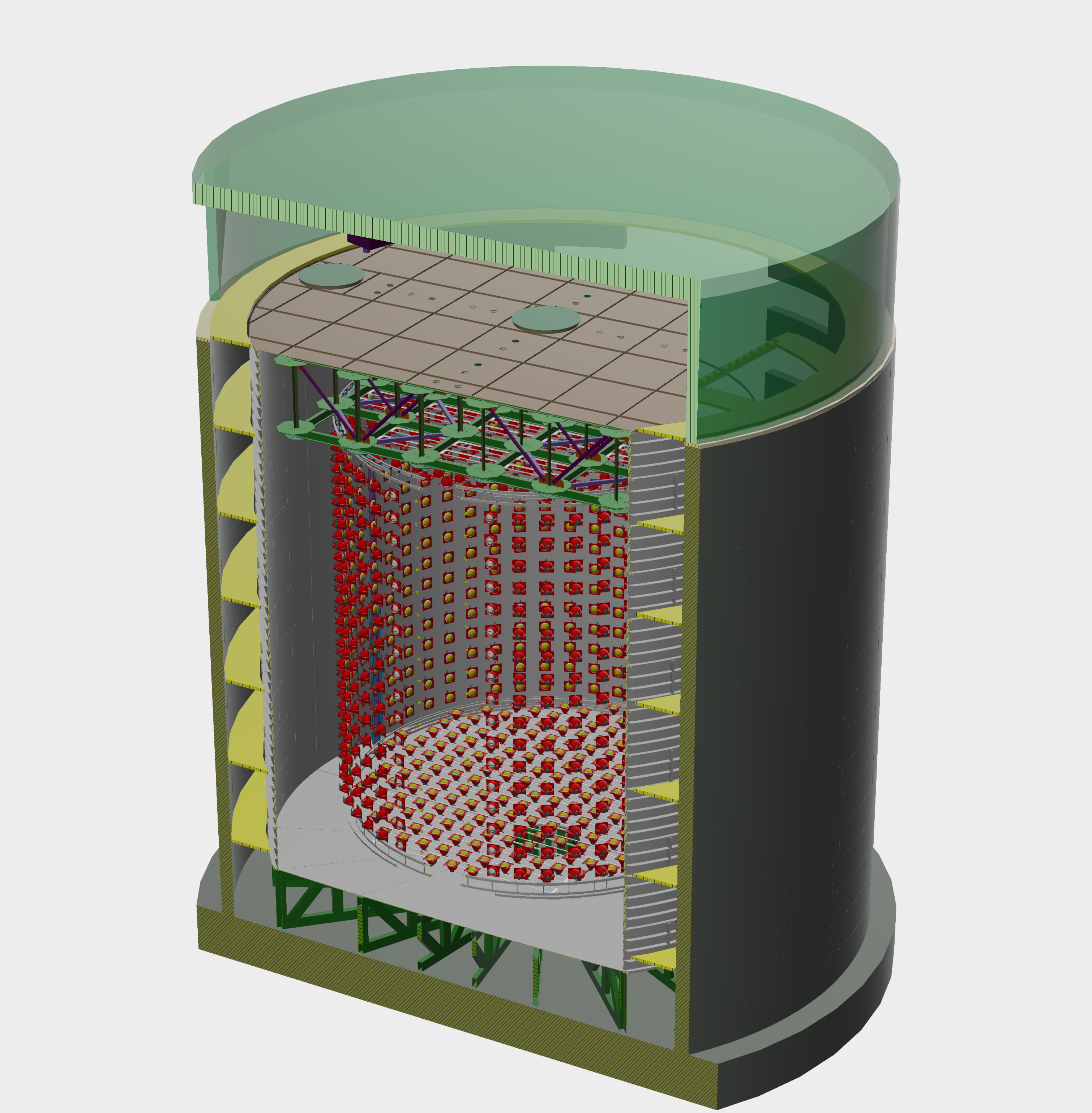
Figure 1: Schematic of the detector design by Jan Boissevain (University of Pennsylvania), showing the tank supported on a steel truss structure and inner PMT support structure.

The expected reactor landscape around Boulby is used for this study. Table 1 shows the reactor sites considered for this study, along with their type, standoff distance, approximate signal rate after data reduction and decommissioning date. At the time of this study, the UK’s advanced gas-cooled reactor (AGR) fleet was due for decommissioning, with the first generation AGR-1 cores by 2024 followed by the second generation AGR-2 fleet by 2028, and Hinkley Point C (a pressurised water reactor (PWR)) had a planned start date of 2026 [29, 30]. Their locations on a map are shown in Fig. 2. Sizewell B, a PWR, was undergoing review for an extension beyond its initially planned end date of 2035 [31].

Table 1: The reactor type, standoff distance, approximate signal rate after data reduction and decommissioning date for the reactors considered in this study. The decommissioning dates are taken from [29, 30, 32]. Sizewell B was under review for a long term extension beyond 2035 at the time of this study [31].

Signal	Number	Type	Standoff	Rate	Decommissioning
	of cores		distance [km]	[per day]	date
Hartlepool	2	AGR-1	26	3	2024
Heysham 1	2	AGR-1	149	0.1	2024
Heysham 2	2	AGR-2	149	0.1	2028
Torness	2	AGR-2	187	0.08	2028
Sizewell-B	1	PWR	306	0.02	after 2035
Hinkley Point C	2	PWR	404	0.03	2086
Gravelines (France)	6	PWR	441	0.03	2031

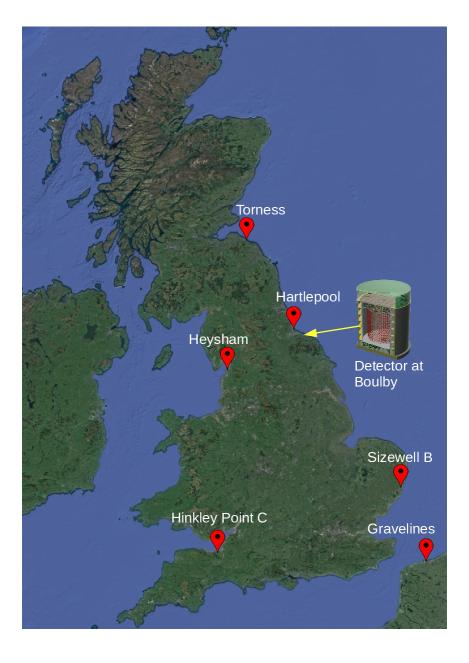
Figure 2: Map showing the location of the detector at Boulby and the reactor sites studied. [33]

IV Method

Two analyses were employed on the same dataset for this study. The data was MC produced in Geant4 [34, 35] for the study in [12]. Signal MC was produced using real reactor data described in Section II.

Several backgrounds are considered for this study, with their approximate rates given in Table 2 [12]. Rates differ slightly depending on the target reactor due to analysis optimizations made during data reduction. Due to the nature of the data reduction performed in analysis, only correlated backgrounds are considered.

Table 2: Backgrounds considered for this study and their approximate rates per day [12].

Component	Rate per day
World	0.2
Geo	0.06
9Li	0.02
17N	0.2
Fast Neutrons	0.05

Uncertainties on the signal and background rates used in this study are shown in Table 3.

Table 3: Uncertainties on signals and backgrounds. Data taken from [13, 12, 36].

Component	Uncertainty (%)
Hartlepool	2.5
Heysham	2.0
Torness	2.6
Sizewell B	2.75
Hinkley Point C	3.0
Gravelines	3.4
World	6.0
Geo	25
9Li	0.2
17N	0.2
Fast Neutrons	27

mc for the backgrounds were produced using rates and sources from a combination of literature and previous studies [37, 38, 39, 40, 41, 42, 43, 44, 45, 46, 47, 24, 48, 36, 49, 50]. Data is taken from the output of the LEARN data reduction [12], and backgrounds combined as appropriate.

The impact of both backgrounds and energy resolution are tested by applying energy reconstruction and/or background uncertainties. The energy reconstruction is applied as in [12], where a fit between simulated particle energy and PMT hits is applied. To remove energy resolution effects, the simulated particle energy is used where appropriate.

To apply background uncertainties, it is assumed the background rates are known at the rates observed in [12] with some Gaussian uncertainty. For each bin in the observed spectrum for the target reactor, a rate is drawn from the uncertainty distributions and combined with the reactor rate for that bin. As the background rates can fluctuate up or down due to their uncertainties, when combined with the signal, it can cause the observed signal rates to fluctuate.

To determine the uncertainty on the range caused by background uncertainties and statistical fluctuations, each “observation” is repeated 100 times.

The impact of both energy resolution and background uncertainties are assessed on the nearer AGRs, but only the energy resolution is included for the more distant PWRs due to the small signal which is obscured by background uncertainties, as seen in Fig. 3. In the case of the Hartlepool cores, all backgrounds are applied including their uncertainties, and full energy reconstruction is used.

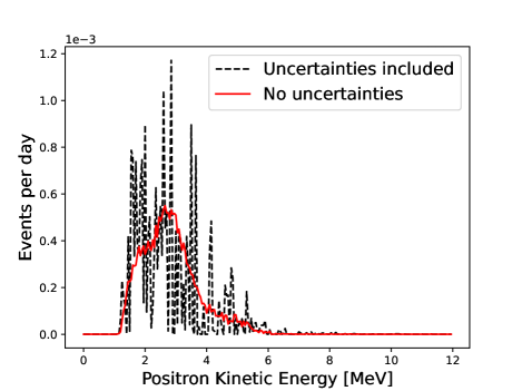
Figure 3: The reconstructed energy spectrum for a single observation of Hinkley Point C with (dashed black) and without (solid red) background uncertainties included after data reduction. A description of the application of background uncertainties is given in the text.

IV.1 Chi-squared

The chi-squared method minimizes the difference between the positron spectrum from analyzed data from [12] and models produced using Equation 4 with the antineutrino energy converted to detected positron kinetic energy. The chi-squared used is given by

$$\chi^{2}=\sum\limits_{i}\frac{(\Phi_{i}-f_{i})^{2}}{f_{i}},$$ (5)

where f_i is the value of Equation 4 for a given distance and the energy corresponding to the i_th bin, and $\Phi_{i}$ is the data content in the i_th energy bin. Both the data and Equation 4 are normalized to a maximum of 1 to mitigate the effects of reactor power. The distance to the reactor is incremented between 0 and 500 km at 0.1 km intervals and the value of Equation 5 is minimized to yield an “observed” range for a reactor.

IV.2 Fourier transform

As shown in Equation 7, the oscillation probability of one neutrino flavor state to another is proportional to sin${}^{2}(\frac{1.27\Delta m_{ij}^{2}L}{E_{\bar{\nu}}})$, where $\Delta$m${}^{2}_{ij}$ is the square of the mass difference between flavors i and j, L is the distance the antineutrino travels and E${}_{\bar{\nu}}$ is the energy of the antineutrino. As such, the oscillation of neutrino flavor is dependent on the distance and energy domains. As the kinetic energy of the positrons from IBD can be measured and the antineutrino energy determined from this, a FT can be used to switch from antineutrino energy to the distance of travel.

The survival probability of an electron flavor neutrino is given in Equation 6.

$$P(L,E_{\bar{\nu}})=1-P_{ex},$$ (6)

where

$$P_{ex}=\cos^{4}(\theta_{13})\sin^{2}(2\theta_{12})\sin^{2}\Big{(}\frac{1.27\Delta m^{{}^{2}}_{21}L}{E_{\bar{\nu}}}\Big{)}+$$ (7)

$$\cos^{2}(\theta_{12})\sin^{2}(2\theta_{13})\sin^{2}\Big{(}\frac{1.27\Delta m^{{}^{2}}_{31}L}{E_{\bar{\nu}}}\Big{)}+$$

$$\sin^{2}(\theta_{12})\sin^{2}(2\theta_{13})\sin^{2}\Big{(}\frac{1.27\Delta m^{{}^{2}}_{32}L}{E_{\bar{\nu}}}\Big{)},$$

assuming charge-parity-time invariance [13]. Here, $\theta_{ij}$ is the mixing angle between flavors i and j.

As the oscillation probability depends on sin${}^{2}(\frac{1.27\Delta m_{ij}^{2}L}{E_{\bar{\nu}}})$, the identity sin${}^{2}(\theta)$ = $\frac{1-\mathrm{cos}(2\theta)}{2}$ can be used to express the FT as

$$\text{FCT}(L)\propto\int_{\frac{1}{E_{min}}}^{\frac{1}{E_{max}}}f(L,E_{\bar{\nu}})\;\text{cos}\left(2\times\frac{1.27\Delta m_{ij}^{2}L}{E_{\bar{\nu}}}\right)\,d\frac{1}{E_{\bar{\nu}}}.$$ (8)

Here, Equation 8 is defined as a Fourier cosine transform (FCT). A phase shift can be applied for a Fourier sine transform (FST), shown in Equation 9.

$$\text{FST}(L)\propto\int_{\frac{1}{E_{min}}}^{\frac{1}{E_{max}}}f(L,E_{\bar{\nu}})\;\text{sin}\left(2\times\frac{1.27\Delta m_{ij}^{2}L}{E_{\bar{\nu}}}\right)\,d\frac{1}{E_{\bar{\nu}}}.$$ (9)

Both Equation 8 and Equation 9 include terms not associated with neutrino oscillations within the term $f(L,E_{\bar{\nu}})$. To isolate the oscillation terms, a spectrum where no oscillation is assumed is simulated i.e. the model in Equation 4 but only including the terms from Equation 1 and Equation 3. A FT is performed on this spectrum and it is then subtracted from the one performed on the original data. The effect of this can be seen clearly in Fig. 4, where the peak associated with factors not related to neutrino oscillation are removed.

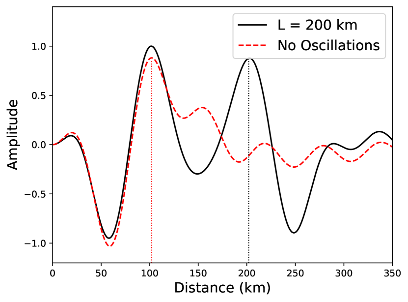
(a)

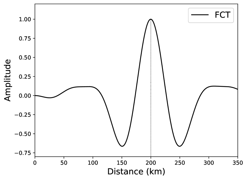
(b)

Figure 4: Comparison of the Fourier transform for oscillations (black solid) and no oscillations (red dashed) in the reactor spectrum modeling for a 200 km standoff distance (a), and the subtraction of the no oscillation situation from the original reactor model for the same reactor standoff (b). The reactor model has peaks for 100 km and 200 km before the subtraction, and only the expected peak at 200 km after subtraction.

As the distance is varied, the peak amplitude of the FCT and the zero amplitude values of the FST are the points of interest that correspond to the “observed” range. Fig. 5 shows how the FCT and FST can be used in combination to reduce the possible ranges responsible for the detected spectrum by only considering the regions in which they match.

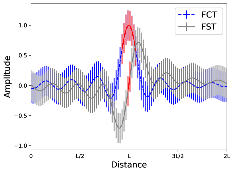
Figure 5: The combination of an FCT (blue dashed) and FST (gray solid) allows the area of interest (red solid) to be narrowed down to reduce uncertainties by comparing where the maxima of the FCT and zeroes of the FST occur at matching distances.

Due to the detector resolution, only the $\theta_{12}$ oscillation pattern can be resolved. As such, the FTs are normalized to the $\theta_{12}$ term, and $\theta_{13}$ and $\theta_{23}$ are neglected. This creates a lower limit to the range that can be observed with this method, as at least one full wavelength of the oscillation pattern must be visible in the spectrum for a FT to work.

Although detailed analysis has been performed on specific reactors, this is illustrative only due to the expected decommissioning of many of the observed cores. As such, a scan over generic scenarios has been carried out up to a range of 500 km to show the potential of this analysis, with the results in Fig. 6. A lower limit of approximately 80 km can be seen due to the requirement of a full wavelength of the oscillation pattern.

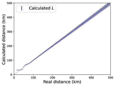
Figure 6: The analytical range of reactors with distance using the Fourier transform analysis. The Fourier transform relies on resolving the $\theta_{12}$ oscillations, which are not obviously present at ranges below 100 km, as the $\theta_{13}$ oscillations are smaller than the detector’s energy resolution.

V Results

V.1 Chi-squared

For the minimum chi-squared method, a single analysis was performed. This was the ranging of the EDF Hartlepool reactor with all limitations, such as complete backgrounds including uncertainties and detector effects, considered as part of the LEARN analysis chain in [12]. The obtained range, shown in comparison to the true range in Table 4, is 50% from the expected value.

Table 4: Observed distance in km for the Chi-squared method for Hartlepool.

	True	Chi-squared
Distance (km)	26	39 $\pm$ 1

Hartlepool is the dominant signal after data reduction, so assuming all backgrounds are known only improves the observed range slightly to $\approx$ 35 km. The biggest cause of the discrepancy between the observed and true range is the depletion of the low energy events caused by the data reduction in [12]. To remove the numerous radioactive background events, low energy cuts are applied. This, alongside the detector’s increasing efficiency with energy, cause the spectrum to shift to higher energy and impact the observed range. The impact on the observed spectrum in comparison to the models for the true range at 26 km and observed range at 39 km can be seen in Fig. 7(a) and Fig. 7(b) respectively.

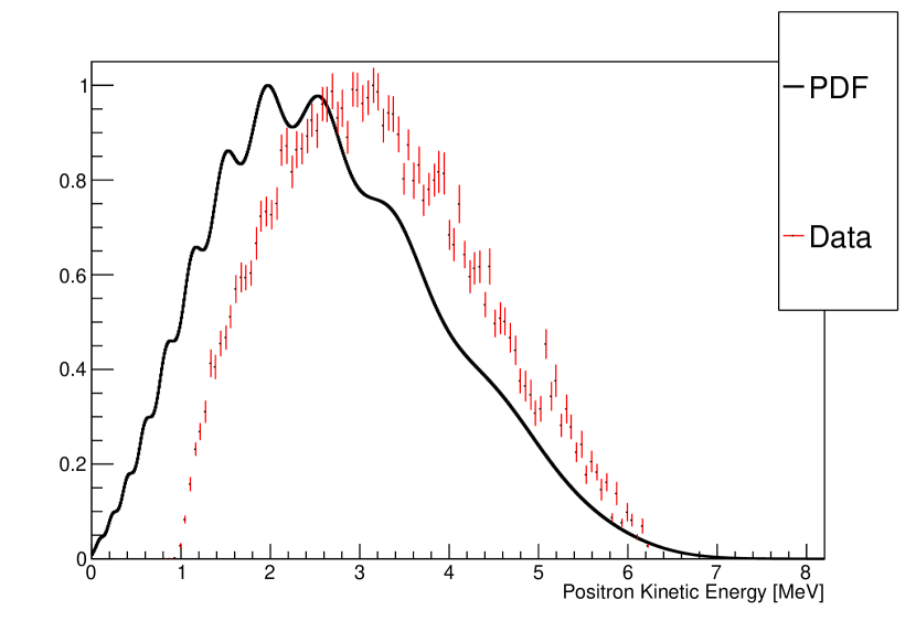
(a)

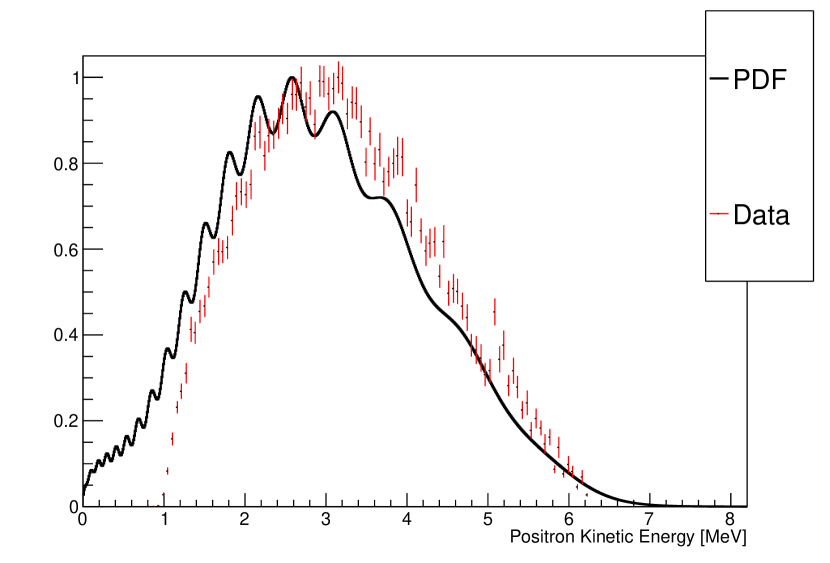
(b)

Figure 7: The comparison of the analyzed Hartlepool reactor complex data (red points) and models (black solid line) for the (a) true range and (b) observed range. The shift to higher energy in the data can be seen. This shift limits the ability to range the reactor as the shape of the spectrum is what is used to determine the range.

The observation time needed to range Hartlepool to this accuracy is 40 months, with the uncertainty dropping to the level in Table 4 by around 50 months, as demonstrated by Fig. 8.

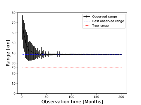
Figure 8: The observed range of the Hartlepool reactor complex with observation time.

Due to the simplicity of the method, and the need for a signal-dominated spectrum, this analysis is not appropriate for higher-background situations such as more distant reactors. Further analysis would be required to isolate a complete reactor spectrum for this method to be effective at larger distances.

V.2 Fourier transform

The Fourier transform (FT) method is applied in four possible scenarios on five reactor complexes. The scenarios are combinations of including background uncertainties and detector energy resolution.

The results of the FT method shown in Table. 5 show that for reactors at large distances, the range can be determined when the detector’s energy resolution is accounted for. However, reactors beyond 300 km do not have a large enough signal to be ranged effectively when background uncertainties are included.

The two nearer reactors, AGRs at Heysham and Torness, can be ranged close to the true value when background uncertainties are included.

Table 5: Observed distance in km for the Fourier transform method for the situations where true energy and reconstructed energy are used. Inclusion of background uncertainties is compared to the situation of zero background uncertainty. Situations with a slash are deemed impossible to range due to background uncertainties dominating.

Situation			Range [km]
	Heysham 2	Torness	Sizewell B	Hinkley Point C	Gravelines
True Range	149	187	304	404	441
No Background, True Energy	148 $\pm$ 4	188 $\pm$ 5	306 $\pm$ 8	403 $\pm$ 11	440 $\pm$ 11
No Background, Reconstructed Energy	157 $\pm$ 4	195 $\pm$ 5	307 $\pm$ 8	397 $\pm$ 11	432 $\pm$ 11
Background Uncertainty, True Energy	156 $\pm$ 6	177 $\pm$ 10
Background Uncertainty, Reconstructed Energy	155 $\pm$ 5	171 $\pm$ 9

As shown in Fig. 6, reactors within approximately 80 km of the detector cannot be accurately ranged by the FT method. As such, the EDF Hartlepool cores were not ranged as part of this analysis.

The FT for Heysham 2 with background uncertainties and with energy reconstruction applied is shown by Fig. 9. The maximum for the FCT yields an accurate range, but with an uncertainty of $\pm$ 15 km. The FST is able to reduce this uncertainty significantly to $\pm$ 6, shown in Table 5.

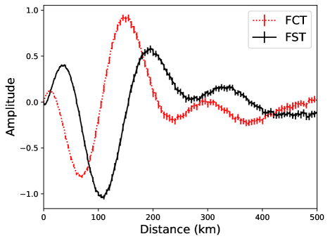
Figure 9: The Fourier transform, in sine (black solid) and cosine (red dotted), for Heysham 2 with background uncertainties and energy resolution effects.

Due to the low event rates for the distant reactors, it takes over 50 years of observation time to be able to range the Heysham complex, and significantly longer for the more distant reactors.

VI Discussion

The results of both methods show the potential of using neutrino oscillation to determine the distance to an observed reactor, as well as the use of extending the analysis in [12] to include a spectral analysis. The two analyses presented complement each other well, with the minimum chi-squared analysis allowing nearby reactors with a large signal contribution to be ranged, and the Fourier transform (FT) method allowing the ranging of more distant reactors.

Despite showing potential, there are strong limitations to both methods. While the chi-squared method can handle lower energy resolutions for mid-field reactors, the energy threshold and detector efficiency strongly limits the utilization of lower energy events. This causes the discrepancy between the true and observed range for the Hartlepool reactors.

The FT method is able to range reactors in more complex scenarios. However, the event rate for these distant reactors results in this taking a long time, in excess of 50 years, and therefore being impractical.

This detector configuration is not able to make the best use of spectral analysis. A potential solution is using gadolinium-loaded liquid scintillator. This would lower the energy threshold, boost detector efficiency at low energies and improve energy resolution. In principle, this could allow the FT method to work at much shorter ranges by resolving the $\theta_{13}$ oscillations or allow the chi-squared method to range Hartlepool with much more accuracy.

VII Conclusions

An attempt at extending the rate-only analysis of nuclear fission reactor antineutrinos in [12] has been made by using two methods of spectral analysis with the aim of determining the distance between a reactor and a detector. The simulated detector used is a 22 m height and diameter right cylinder with a 9 m inner PMT support structure and a 15% PMT coverage. The detector is filled with gadolinium-doped water-based liquid scintillator, and is located at the Science & Technology Facilities Council (STFC) Boulby Underground Laboratory.

The analyses show potential to range real reactor signals, but are significantly limited by the detector design. A minimum chi-squared analysis is able to range nearby reactors which produce a dominant signal well within the lifetime of this kind of detector, with the EDF Hartlepool reactor ranged to 50% of its true distance. A Fourier transform analysis is able to handle reactors at much larger standoff distances, up to 180 km when background uncertainties are included. However, this would take a very large amount of time due to the low event rate.

With both analyses, the fundamental issue is the detector’s performance. An order of magnitude increase in signal rate is needed to range the Heysham 2 cores at 149 km within a detector lifetime, and the energy thresholds and detector efficiency limit the ranging of more local reactors. Using gadolinium-doped liquid scintillator could offer a solution as it would improve energy resolution, lower the threshold and improve low energy efficiency.

Due to performance issues, the gadolinium-doped WbLS detection medium is not appropriate to use in determining the distance to operating reactors. However, the analyses developed could be used with a more sensitive detector for this purpose.

Author contributions

The initial proposal of both reactor ranging in general and the application of a Fourier transform came from J. G. Learned.

Monte Carlo simulations produced by S. Wilson with input from L. Kneale.

The LEARN analysis for data reduction developed by S. Wilson with input from J. Armitage, N. Holland and T. Appleyard. Sections of the data reduction, such as the analytic post-muon veto and radionuclide calculations were developed by L. Kneale.

The chi-squared analysis was initially developed by J. Armitage, later being taken on by S. Wilson. The Fourier transform was developed by C. Cotsford.

C. Cotsford drafted Section IV.2, with S. Wilson drafting the remainder of the paper.

References

- NNSA [2021] NNSA, Prevent, Counter, and Respond — NNSA’s Plan to Reduce Global Nuclear Threats (2021).
- United Nations [1970] United Nations, Treaty on the Non-Proliferation of Nuclear Weapons (1970).
- International Atomic Energy Agency [1997] International Atomic Energy Agency, Model protocol additional to the agreements(s) between the state(s) and the international atomic energy agency for the application of safeguards (1997).
- Eguchi et al. [2003] K. Eguchi, S. Enomoto, K. Furuno, J. Goldman, H. Hanada, H. Ikeda, K. Ikeda, K. Inoue, K. Ishihara, W. Itoh, et al. (KamLAND Collaboration), Phys. Rev. Lett. 90, 021802 (2003).
- Abe et al. [2012] Y. Abe, C. Aberle, T. Akiri, J. C. dos Anjos, F. Ardellier, A. F. Barbosa, A. Baxter, M. Bergevin, A. Bernstein, Bezerra, et al. (Double Chooz Collaboration), Phys. Rev. Lett. 108, 131801 (2012).
- Cowan et al. [1956] C. L. Cowan, F. Reines, F. B. Harrison, H. W. Kruse, and A. D. McGuire, Science 124, 103 (1956), https://www.science.org/doi/pdf/10.1126/science.124.3212.103 .
- Cowan and Reines [1956] C. L. Cowan and F. Reines, Nature 178, 446 (1956).
- Kuroda et al. [2012] Y. Kuroda, S. Oguri, Y. Kato, R. Nakata, Y. Inoue, C. Ito, and M. Minowa, Nucl. Instrum. Methods Phys. Res. A 690, 41 (2012).
- Haghighat et al. [2020] A. Haghighat, P. Huber, S. Li, J. M. Link, C. Mariani, J. Park, and T. Subedi, Phys. Rev. Appl. 13, 034028 (2020).
- Ozturk [2020] S. Ozturk, Nucl. Instrum. Methods Phys. Res. A 955, 163314 (2020).
- Akindele et al. [2021] T. Akindele, N. Bowden, R. Carr, A. J. Conant, M. Diwan, A. Erickson, M. P. Foxe, B. L. Goldblum, P. Huber, I. Jovanovic, et al. 10.2172/1826602 (2021).
- Kneale et al. [2022] L. Kneale, S. T. Wilson, T. Appleyard, J. Armitage, N. Holland, and M. Malek, Sensitivity of an antineutrino monitor for remote nuclear reactor discovery (2022).
- Dye and Barna [2021] S. Dye and A. Barna, Global antineutrino modeling for a web application (2021).
- International Atomic Energy Agency [2022] International Atomic Energy Agency, Power Reactor Information System (PRIS) (2022).
- Bogetic et al. [2023] S. Bogetic, R. Mills, A. Bernstein, J. Coleman, A. Morgan, and A. Petts, Anti-neutrino flux from the EdF Hartlepool nuclear power plant (2023).
- Huber [2011] P. Huber, Phys. Rev. C 84, 024617 (2011).
- Mueller et al. [2011] T. A. Mueller, D. Lhuillier, M. Fallot, A. Letourneau, S. Cormon, M. Fechner, L. Giot, T. Lasserre, J. Martino, G. Mention, A. Porta, and F. Yermia, Phys. Rev. C 83, 054615 (2011).
- Vogel and Beacom [1999] P. Vogel and J. F. Beacom, Phys. Rev. D 60, 053003 (1999).
- Strumia and Vissani [2003] A. Strumia and F. Vissani, Phys. Lett. B 564, 42 (2003).
- Ricciardi et al. [2022] G. Ricciardi, N. Vignaroli, and F. Vassani, J. High. Energ. Phys 2022, 212 (2022).
- Maki et al. [1962] Z. Maki, M. Nakagawa, and S. Sakata, Prog. Theor. Phys. 28, 870 (1962).
- Branco and Rebelo [2009] G. C. Branco and M. N. Rebelo, Phys. Rev. D 79, 013001 (2009).
- Workman et al. [2022] R. L. Workman, V. D. Burkert, V. Crede, E. Klempt, U. Thoma, L. Tiator, K. Agashe, G. Aielli, B. C. Allanach, C. Amsler, et al. (Particle Data Group), Prog. Theor. Exp. Phys. 2022, 10.1093/ptep/ptac097 (2022), 083C01.
- Robinson et al. [2003] M. Robinson, V. Kudryavtsev, R. Lüscher, J. McMillan, P. Lightfoot, N. Spooner, N. Smith, and I. Liubarsky, Nucl. Instrum. Methods Phys. Res. A 511, 347 (2003).
- Yeh et al. [2011] M. Yeh, S. Hans, W. Beriguete, R. Rosero, L. Hu, R. Hahn, M. Diwan, D. Jaffe, S. Kettell, and L. Littenberg, Nucl. Instrum. Methods Phys. Res. A 660, 51 (2011).
- Zsoldos et al. [2022] S. Zsoldos, Z. Bagdasarian, G. D. O. Gann, A. Barna, and S. Dye, Euro. Phys. J. C 82, 10.1140/epjc/s10052-022-11106-1 (2022).
- Beacom and Vagins [2004] J. F. Beacom and M. R. Vagins, Phys. Rev. Lett. 93, 171101 (2004).
- Abe et al. [2021] K. Abe, C. Bronner, Y. Hayato, K. Hiraide, M. Ikeda, S. Imaizumi, J. Kameda, Y. Kanemura, Y. Kataoka, S. Miki, et al. (Super-Kamiokande Collaboration), Nucl. Instrum. Methods Phys. Res. A 1027, 166248 (2021).
- EDF Energy [2022a] EDF Energy, Nuclear Lifetime Management (2022a).
- EDF Energy [2022b] EDF Energy, About Hinkley Point C (2022b).
- EDF Energy [2022c] EDF Energy, Sizewell B starts review to extend operation by 20 years (2022c).
- ASN [2021] ASN, ASN issues a position statement on the conditions for continued operation of the 900 MWe reactors beyond 40 years (2021).
- Google [2022] Google, Google Maps satellite image showing location of nuclear power stations in the UK and northern France (2022).
- Allison et al. [2016] J. Allison, K. Amako, J. Apostolakis, P. Arce, M. Asai, T. Aso, E. Bagli, A. Bagulya, S. Banerjee, G. Barrand, et al., Nucl. Instrum. Methods Phys. Res. A 835, 186 (2016).
- Agostinelli et al. [2003] S. Agostinelli, J. Allison, K. Amako, J. Apostolakis, H. Araujo, P. Arce, M. Asai, D. Axen, S. Banerjee, G. Barrand, et al., Nucl. Instrum. Methods Phys. Res. A 506, 250 (2003).
- Mei and Hime [2006] D.-M. Mei and A. Hime, Phys. Rev. D 73, 053004 (2006).
- Kneale [2021] L. Kneale, Coincidence-based reconstruction and analysis for remote reactor monitoring with antineutrinos, Ph.D. thesis, University of Sheffield (2021).
- Marti et al. [2020] L. Marti, M. Ikeda, Y. Kato, Y. Kishimoto, M. Nakahata, Y. Nakajima, Y. Nakano, S. Nakayama, Y. Okajima, A. Orii, et al., Nucl. Instrum. Methods Phys. Res. A 959, 163549 (2020).
- Haselschwardt et al. [2019] S. Haselschwardt, S. Shaw, H. Nelson, M. Witherell, M. Yeh, K. Lesko, A. Cole, S. Kyre, and D. White, Nucl. Instrum. Methods Phys. Res. A 937, 148 (2019).
- Ham [2020] Hamamatsu Photonics K. K. (private communication) (2020).
- Zhang et al. [2016a] T. Zhang, C. Fu, X. Ji, J. Liu, X. Liu, X. Wang, C. Yao, and X. Yuan, JINST 11 (09), T09004.
- Zhang et al. [2016b] Y. Zhang, K. Abe, Y. Haga, Y. Hayato, M. Ikeda, K. Iyogi, J. Kameda, Y. Kishimoto, M. Miura, S. Moriyama, et al. (Super-Kamiokande Collaboration), Phys. Rev. D 93, 012004 (2016b).
- Araújo et al. [2012] H. Araújo, D. Y. Akimov, E. Barnes, V. Belov, A. Bewick, A. Burenkov, V. Chepel, A. Currie, L. DeViveiros, B. Edwards, et al., Astropart. Phys. 35, 495 (2012).
- Li and Beacom [2014] S. W. Li and J. F. Beacom, Phys. Rev. C 89, 045801 (2014).
- Chu et al. [1999] S. Chu, L. Ekström, and R. Firestone, The Lund/LBNL Nuclear Data Search: Table of Radioactive Isotopes (1999).
- TUNL Nuclear Data Evaluation Project [2021] TUNL Nuclear Data Evaluation Project, Energy Level Diagrams (2021).
- Jollet and Meregaglia [2020] C. Jollet and A. Meregaglia, Nucl. Instrum. Methods Phys. Res. A 949, 162904 (2020).
- Wang et al. [2001] Y.-F. Wang, V. Balic, G. Gratta, A. Fassò, S. Roesler, and A. Ferrari, Phys. Rev. D 64, 013012 (2001).
- Tang et al. [2006] A. Tang, G. Horton-Smith, V. A. Kudryavtsev, and A. Tonazzo, Phys. Rev. D 74, 053007 (2006).
- Sutanto et al. [2020] F. Sutanto, O. A. Akindele, M. Askins, M. Bergevin, A. Bernstein, N. S. Bowden, S. Dazeley, P. Jaffke, I. Jovanovic, S. Quillin, et al., Phys. Rev. C 102, 034616 (2020).