A Hierarchical Game-Theoretic Decision-Making for Cooperative Multi-Agent Systems Under the Presence of Adversarial Agents

Abstract.

Underlying relationships among Multi-Agent Systems (MAS) in hazardous scenarios can be represented as Game-theoretic models. This paper proposes a new hierarchical network-based model called Game-theoretic Utility Tree (GUT), which decomposes high-level strategies into executable low-level actions for cooperative MAS decisions. It combines with a new payoff measure based on agent needs for real-time strategy games. We present an Explore game domain, where we measure the performance of MAS achieving tasks from the perspective of balancing the success probability and system costs. We evaluate the GUT approach against state-of-the-art methods that greedily rely on rewards of the composite actions. Conclusive results on extensive numerical simulations indicate that GUT can organize more complex relationships among MAS cooperation, helping the group achieve challenging tasks with lower costs and higher winning rates. Furthermore, we demonstrated the applicability of the GUT using the simulator-hardware testbed - Robotarium. The performances verified the effectiveness of the GUT in the real robot application and validated that the GUT could effectively organize MAS cooperation strategies, helping the group with fewer advantages achieve higher performance.

1. Introduction

Multi-Agent Systems (MAS) (Wooldridge, 2009) that cooperate with each other show Distributed Intelligence, which refers to systems of entities working together to reason, plan, solve problems, think abstractly, comprehend ideas and language, and learn (Parker, 2007). Here, an individual agent is aware of other group members and actively shares and integrates its needs, goals, actions, plans, and strategies to achieve a common goal and benefit the entire group (Yang et al., 2019; Yang, 2022). They can maximize global system utility and guarantee sustainable development for each group member (Shen et al., 2004).

Systems with a wide variety of agent heterogeneity and communication abilities can be studied, and collaborative and adversarial issues can also be combined in a real-time situation (Stone and Veloso, 2000). Under the presence of adversarial agents, opponents can prevent agents from achieving global and local tasks, even impair individual or system necessary capabilities or normal functions (Jun and D’Andrea, 2003). Combining Multi-Agent cooperative decision-making and robotics disciplines, researchers developed the Adversarial Robotics, focusing on autonomous agents operating in adversarial environments (Yehoshua and Agmon, 2015). From the agent’s needs (Yang and Parasuraman, 2020a) and motivations perspective, we can classify an Adversary into two general categories: Intentional adversary (such as an enemy agent, which consciously and actively impairs the agent’s needs and capabilities as depicted in Fig. 1) and Unintentional adversary (like obstacles, which passively threaten agent abilities). In this paper, we focus on the Multi-Agent tasks in the presence of adversarial agents (physical and intentional adversaries present at random locations in the environment).

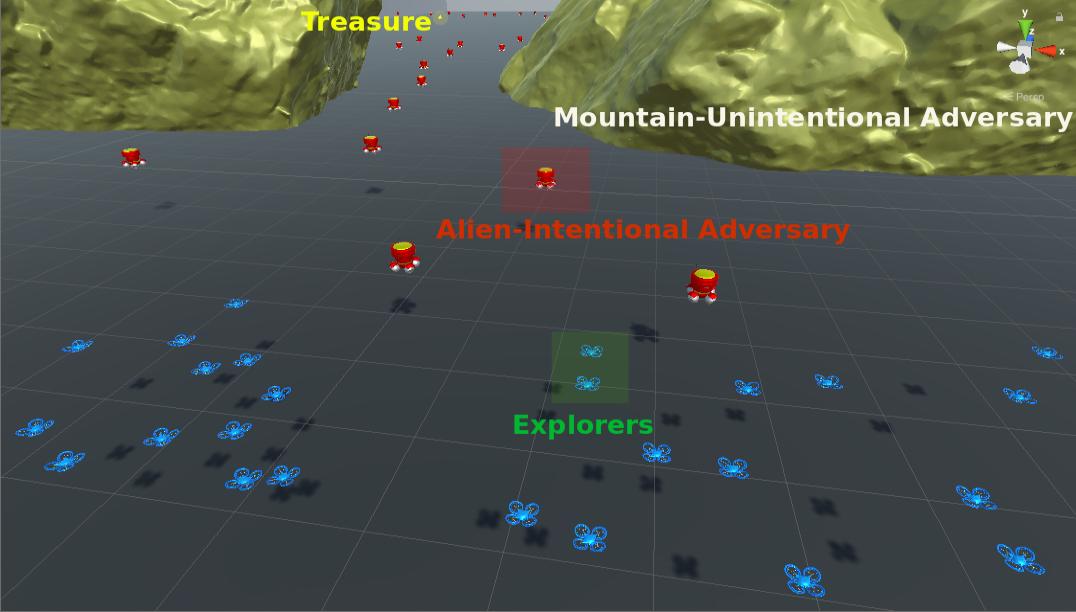
Explore Domain

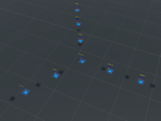
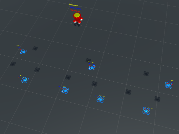
Patrolling

Attacking

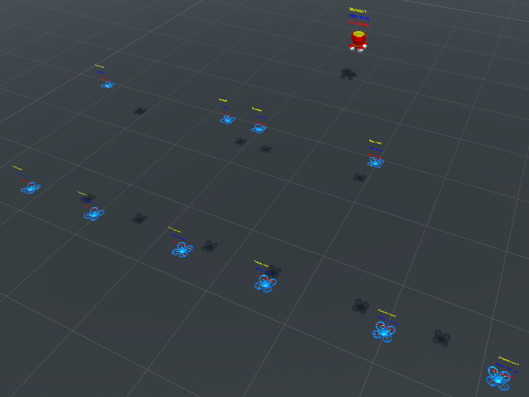
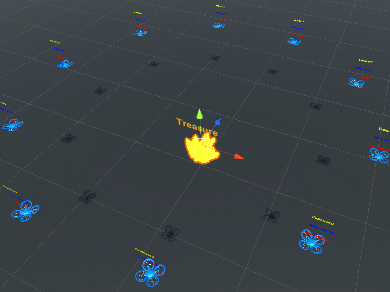
Defending

Final State

Figure 1. Illustration of the game scenario where the Aliens (opponent agents - peer adversaries) block the paths to a target of the Explorers (protagonist agents). Further, the Explorers cooperate to keep different formations in specific situations depicted on the right side.

MAS research domains focus on solving path planning problems for avoiding static or dynamical obstacles in coverage and patrolling (Agmon et al., 2011; Yehoshua and Agmon, 2015) from the unintentional adversary perspective. For intentional (peer) adversaries, the "pursuit domain" (Chung et al., 2011) primarily deals with how to guide one or a group of pursuers to catch one or a group of moving evaders (Makkapati and Tsiotras, 2019). Similarly, the robot soccer domain (Nadarajah and Sundaraj, 2013) deals with how one group of robots wins over another group of robots on a common game element. Foundations for normal-form team games and extensive-form adversarial team games are provided in (von Stengel and Koller, 1997) and (Celli and Gatti, 2018), respectively. From a game-theoretic control perspective, most of the research has focused on single stage games with fixed known agent utilities (Browning et al., 2005), such as distributed control in communication (Zhang et al., 2014) and Multi-Agent task allocation (Bakolas and Lee, 2021). Nevertheless, it is more realistic and practical for MAS to organize more complex relationships and behaviors, achieving given tasks with higher success probability and lower costs in adversarial environments.

Contributions: The paper contributes to the field of Multi-Agent systems through the following ways.

• Firstly, this paper proposes a new hierarchical network model called Game-theoretic Utility Tree (GUT) to achieve cooperative decision-making of team-level Multi-Agent strategies under the presence of adversarial agents.

• Secondly, we present a game of Explorers vs. Aliens, referred to as "Explore Domain" (see Fig. 1), to analyze the MAS performance by balancing the success probability of achieving tasks and system costs by organizing involved agents’ relationships and suitable groups’ strategies in adversarial environments.

• Thirdly, we demonstrate the effectiveness of GUT against the standard decision-making algorithms such as QMIX (Rashid et al., 2018) and greedy approaches in extensive simulations of the Explore Domain. The results indicate that GUT could organize more complex relationships among MAS, helping the group achieve tasks with low costs and high winning probability.

• Finally, to verify the effectiveness of the GUT in the real world (and robotics) applications, we demonstrated the Explore Domain in the Robotarium simulator-hardware multi-robot platform (Pickem et al., 2017).

2. Background and Preliminaries

This section provides a brief background to the Game theory principles used in this paper. Then, we present the agent needs hierarchy based on which the payoff utilities in our game-theoretic approach are designed. Further, we discuss the "Explore Domain" problem.

2.1. Game Theory Basics

Game Theory is the science of strategy, which provides a theoretical framework to conceive social situations among competing players and produce optimal decision-making of independent and competing actors in a strategic setting (Myerson, 2013).

In a non-cooperative game, players compete individually and try to raise their profits alone. Especially in the zero-sum games, their total value is constant and will not decrease or increase, which means that one player’s profit is associated with another loss. In contrast, if different players form several coalitions trying to take advantage of their coalition, that game will be cooperative (Sohrabi and Azgomi, 2020).

If a player chooses to take one action with probability 100%, then the player is playing a pure strategy. For the game’s solutions, if players adopt a Pure Strategy, it will provide maximum profit or the best outcome. Therefore, it is regarded as the best strategy for every player of the game. On the other hand, in a Mixed Strategy, players execute different strategies with the possible outcome through a probability distribution over several actions. In the game theory, the Normal Form describes a game through a matrix, where each player has a set of (mixed) strategies. They select a strategy and play their selections simultaneously. Furthermore, the selection of strategies results in payoff or utility for each player, and its goal in a game is to maximize utility.

Furthermore, Nash Existence Theorem is a theoretical framework, which guarantees the existence of a set of mixed strategies for a finite, non-cooperative game of two or more players in which no player can improve its payoff by unilaterally changing strategy. It guarantees that every game has at least one Nash equilibrium (Jiang and Leyton-Brown, 2009), which means that every finite game has a Pure Strategy Nash Equilibrium or a Mixed Strategy Nash Equilibrium. Moreover, in any normal-form game with constant number of strategies per player, an $\epsilon$-approximate Nash Equilibrium can be computed in time $\mathop{O}(n^{log~{}n/\epsilon^{2}})$, where $n$ is the description size of the game (Daskalakis et al., 2009).

2.2. Agent Needs Hierarchy

In Agent Needs Hierarchy (Yang and Parasuraman, 2020a), the abstract needs of an agent for a given task are prioritized and distributed into multiple levels, each of them preconditioned on their lower levels. At each level, it expresses the needs as an expectation over the corresponding factors/features’ distribution to the specific group (Yang and Parasuraman, 2020b).

Specifically, it defines five different levels of agent needs similar to Maslow’s human needs pyramid (Yang and Parasuraman, 2021). The lowest (first) level is the safety features of the agent (e.g., features such as collision detection, fault detection, etc., that assure safety to the agent, human, and other friendly agents in the environment). The safety needs (Eq. (1)) can be calculated through its safety feature’s value and corresponding safety feature’s probability based on the current state of the agent. After satisfying safety needs, the agent considers its basic needs (Eq. (2)), which includes features such as energy levels, data communication levels that help maintain the basic operations of that agent. Only after fitting the safety and basic needs, an agent can consider its capability needs (Eq. (3)), which are composed of features such as its health level, computing (e.g., storage, performance), physical functionalities (e.g., resources, manipulation), etc.

At the next higher level, the agent can identify its teaming needs (Eq. (4)) that accounts the contributions of this agent to its team through several factors (e.g., heterogeneity, trust, actions) that the team needs so that they can form a reliable and robust team to successfully perform a given mission.

Ultimately, at the highest level, the agent learns some skills/features to improve its capabilities and performance in achieving a given task, such as Reinforcement Learning. The policy features (Q table or reward function) are accounted into its learning needs expectation (Eq. (5)). The expectation of agent needs at each level are given below:

(1) $$\begin{split}Safety~{}~{}Needs:N_{s_{j}}=\sum_{i=1}^{s_{j}}S_{i}\cdot\mathbb{P}(S_{i}|X_{j},T);\end{split}$$

(2) $$\begin{split}Basic~{}~{}Needs:N_{b_{j}}=\sum_{i=1}^{b_{j}}B_{i}\cdot\mathbb{P}(B_{i}|X_{j},T,N_{s_{j}});\end{split}$$

(3) $$\begin{split}Capability~{}Needs:N_{c_{j}}=\sum_{i=1}^{c_{j}}C_{i}\cdot\mathbb{P}(C_{i}|X_{j},T,N_{b_{j}});\end{split}$$

(4) $$\begin{split}Teaming~{}~{}Needs:N_{t_{j}}=\sum_{i=1}^{t_{j}}T_{i}\cdot\mathbb{P(}T_{i}|X_{j},T,N_{c_{j}});\end{split}$$

(5) $$\begin{split}Learning~{}~{}Needs:N_{l_{j}}=\sum_{i=1}^{l_{j}}L_{i}\cdot\mathbb{P(}L_{i}|X_{j},T,N_{t_{j}});\end{split}$$

Here, $X_{j}=\{P_{j},C_{j}\}$ $\in$ $\Psi$ is the combined state of the agent $j$ with $P_{j}$ being the perceived information by that agent and $C_{j}$ representing the communicated data from other agents. $T$ is the assigned task (goal or objective). $S_{i}$, $B_{i}$, $C_{i}$, $T_{i}$, and $L_{i}$ are the utility values of corresponding feature/factor $i$ in the corresponding levels - Safety, Basic, Capability, Teaming, and Learning, respectively. $s_{j}$, $b_{j}$, $c_{j}$, $t_{j}$, and $l_{j}$ are the sizes of agent $j$’s feature space on the respective levels of needs.

The collective need of an agent $j$ is expressed as the union of needs at all the levels in the needs hierarchy as in Eq. (6) .

(6) $$N_{j}=N_{s_{j}}\cup N_{b_{j}}\cup N_{c_{j}}\cup N_{t_{j}}\cup N_{l_{j}}$$

More specifically, the set of agent needs in a Multi-Agent System can be regarded as a kind of motivation or requirements for cooperation between agents to achieve a specific group-level task.

2.3. Adversarial Agent Definition

A friendly (ally) agent can contribute to the team, decreasing the individual needs of the team members, while an adversary can harm the team, increasing the overall needs of every team member. Based on this concept, we define an agent $R_{1}$ as adversary or friendly with respect to an agent $R_{2}$ as follows. For a certain state $\psi$ $\in$ $\Psi$, the agent $R_{1}$ is fulfilling a task $T$. Supposing the current needs of $R_{1}$ is $N_{{R_{1}}}(\psi,T)$. Considering another agent $R_{2}$ entering the $R_{1}$’s observation space, the needs of $R_{1}$ can be represented as $N_{{R_{1}}}(\psi\cup R_{2},T)$ under the presence of the agent $R_{2}$. The following equations define the relationship between $R_{1}$ and $R_{2}$:

(7) $$N_{{R_{1}}}(\psi\cup R_{2},T)-N_{{R_{1}}}(\psi,T)>0; (Adversary)$$

(8) $$N_{{R_{1}}}(\psi\cup R_{2},T)-N_{{R_{1}}}(\psi,T)<0; (Friendly)$$

(9) $$N_{{R_{1}}}(\psi\cup R_{2},T)-N_{{R_{1}}}(\psi,T)=0. (Neutral)$$

Definition 1 (Adversary).

If the needs of $R_{1}$ increase when $R_{2}$ is present, then $R_{1}$ regards $R_{2}$ as an Adversary (Eq. (7)).

Definition 2 (Friendly).

If the needs of $R_{1}$ decrease when $R_{2}$ is present, then $R_{1}$ sees $R_{2}$ as a friendly agent (Eq. (8)).

Definition 3 (Neutral).

If the needs of $R_{1}$ do not change because of $R_{2}$’s presence, then $R_{2}$ is neutral to $R_{1}$ (Eq. (9)).

2.4. Explore Domain Problem

In this paper, to simplify theoretical analysis and numerical calculations, we consider an exemplar problem domain called Explore domain, which is described below. In Explore Domain, $\alpha$ number of agents (called Explorers hereafter) are performing a task $T$, which is to explore an environment and collect rewards by reaching treasure locations. Supposing there are $\beta$ number of (intentional) adversaries (called Aliens hereafter). Explorers can choose a strategy $s_{e}$ from their strategy space $S_{e}$ and aliens can choose a strategy $s_{a}$ from their strategy space $S_{a}$. We assume both these strategy spaces are known to the Explorer agents. We also assume that the Aliens do not have a cooperation strategy, and each Alien acts independently on its own.

Let $C_{i}$ represent the system costs of explorer $i$ to perform this task and $W$ denote the success probability (win rate) of the explorer team under the presence of alien(s). We model this as a bi-objective optimization problem (Eq. (10)) of finding an optimal collective team strategy for the explorers $s_{e}^{*}\in S_{e}$ under the premise of maximizing success $W$ (against aliens) while minimizing costs $C$ using the collective needs of the explorers $N_{e}=\sum_{i=1}^{\alpha}N_{i}$.

(10) $$s_{e}^{*}=\underset{s_{e}\in S_{e}}{\operatorname*{arg\,max}}[W(s_{e}|T,S_{a},N_{e})-\sum_{i=1}^{\alpha}C_{i}(s_{i}|T,s_{e},N_{i})].$$

Without an adversary, the problem shrinks to a typical exploration problem (optimizing $C$ alone) (Kim, 2018), and without a task $T$, the problem shrinks to a typical non-cooperative zero-sum game problem (optimizing $W$ alone) (Myerson, 2013).

The proposed problem can be applied to other Real-Time Strategy (RTS) games, such as air combat and StarCarft, and cooperative Multi-Agent/robot mission, like urban search and rescue (USAR) (Yang and Parasuraman, 2020b), pursuit-evasion game (Chung et al., 2011) and robot soccer (Nadarajah and Sundaraj, 2013). These domains involve both ally agents and opponent agents (intentional adversaries), and the nature of the strategies the agents or the team can take can allow dissolving the high-level group strategies into primitive or atomic actions. For instance, in Star Craft (Vinyals et al., 2019), the strategies a player can make can be composed of the following primitives: What to do? (e.g., Build, Move, Attack, etc.); Who to perform? (which player to execute this action or which opponent to attach, etc.); Where? (physical location or point of interest); When? (immediately or delayed or how long); etc.

3. Proposed GUT Approach

In the following description, we ground the description of the decision-making process with GUT using the "Explore domain" as an example. Fig. 2 outlines the structure of the Game-theoretic Utility Tree (GUT) and its computation units distributed in each level. First, the game-theoretic module (Fig. 2 (a)) calculates the nash equilibrium based on the utility values $(u_{11},...,u_{nm})$ of corresponding situations, $(p_{1},...,p_{nm})$ presenting the probability of each situation. Then, through the conditional probability (CP) module (Fig. 2 (b)), the CP of each situation can be described as $(p_{i1},...,p_{inm})$, where $p_{inm}=(p_{nm}|p_{i-1}),~{}i,n,m\in Z^{+}$.

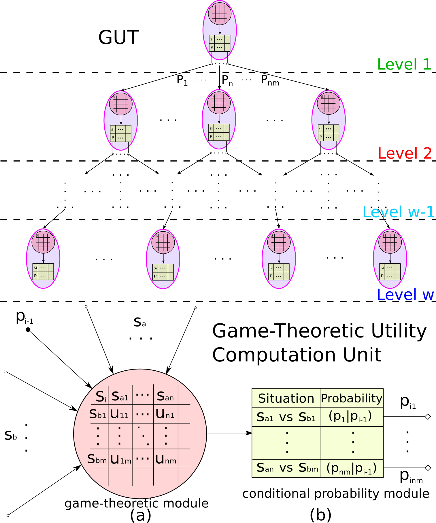
Figure 2. Structure of the Game-theoretic Utility Tree (GUT).

To tackle intentional adversaries, agents first decompose the specific group strategy into several independent sub-strategies based on the same category of individual low-level primitives or atomic operations. Then, through calculating various Nash equilibrium based on different situation utility values in each level’s Game-theoretic Utility Computation Units, agents can get optimal or suboptimal strategy sets tackling the current status according to Nash Existence Theorem.

From the task execution perspective, the GUT can be regarded as a Task-Oriented Decision Tree. It decomposes a big game into several sub-games with conditional dependence in each level, which organizes agents’ strategies and presents more complex behaviors adapting to adversarial environments.

We formulate the decision-making problem as a zero-sum game between two groups of agents when both groups are adversaries to each other, as per the Definition 4. Let A and B represent the group of ally agents and an adversary agent, respectively. The simultaneous normal-form game representing the non-cooperative game between ally and adversaries is a game structure G=$\langle\{s_{A},s_{B}\},\{N_{A},N_{B}\}\rangle$. The theoretical guarantees to prove the effectiveness of the GUT solution for the game G is provided in Theorem 1 below.

Theorem 1 (GUT Decision).

Supposing the GUT for the ally group has w levels of action decomposition together, making a group strategy $s_{A}=\{s_{A}^{1},s_{A}^{2},...,s_{A}^{w}\}$, where $s_{A}^{i}$ represents the $i^{th}$ level sub-strategy in the ally group strategy space. Then, we can show that agent group A using GUT against adversary B will have at least one dominant strategy series $s_{A}^{*}=(s_{A}^{1}*,s_{A}^{2}*,...,s_{A}^{w}*)$, which will enable agents A collectively execute an optimal strategy $s_{A}^{*}$ against adversary B, promising a solution to the problem in Eq. (10).

Proof.

For w-level GUT, supposing game G_i is the level i of GUT describing the corresponding zero-sum game solved using the payoff (utility) values based on the features in the needs hierarchy corresponding to the level of the GUT. To prove the theorem, we will first prove that at each level $i$, the game-theoretic computation units produce optimal strategies. Then, we will show that by composing strategies at each level, the GUT produces the optimal strategy for the team.

Let the size of (team) strategy space of agents in group A within the level $i$ of GUT is l_i and that of agent B is m_i. For GUT-based decision, the zero-sum game at each level is

(11) $$G_{i}=\langle\{s_{A}^{i},s_{B}^{i}\},\{N_{A_{i}},N_{B_{i}}\}\rangle,i\in w.$$

Here, $N_{A_{i}}$ is the needs/utility values of group A at a level $i$ in the GUT. Based on the needs of agent (Eq. (6)), the expectation on the utilities (payoff values) at GUT level $i$ of group A is

(12) $$\mathbb{E}(U^{i})=(u_{gk}^{i})_{l_{i}\times m_{i}}=\sum_{j=1}^{|A|}N^{j}_{A_{i}}(\psi\cup B,T|s_{A}^{i}=g,s_{B}^{i}=k).$$

where, $\psi$ is the combined state perceived by the Multi-Agent group A (with group size $|A|$) executed through the sequence of strategies $s_{A}$, $1\leq g\leq l_{i}$ and $1\leq k\leq m_{i}$. Here, the payoff values depend on the agents’ collective needs of the group.

According to Nash Existence Theorem, it guarantees the existence of a set of mixed strategies for finite, non-cooperative games of two or more players in which no player can improve his payoff by unilaterally changing strategy. So every finite game has a Pure Strategy Nash Equilibrium or a Mixed Strategy Nash Equilibrium. The process can be formalized as two steps:

a. Compute Pure Strategy Nash Equilibrium

We can present the agents’ utility matrix as Eq. (13):

(13) $$\left[\begin{matrix}u_{11}&u_{12}&\cdots&u_{1m_{i}}\\ u_{21}&u_{22}&\cdots&u_{2m_{i}}\\ \vdots&\vdots&\ddots&\vdots\\ u_{l_{i}1}&u_{l_{i}2}&\cdots&u_{l_{i}m_{i}}\\ \end{matrix}\right]$$

The row and column correspond to the utilities of agent $A$ and $B$, respectively. We can compute the maximum and minimum values of the two lists separately by calculating each row’s minimum value and each column’s maximum value.

(14) $$\max\limits_{1\leq k\leq m_{i}}\min\limits_{1\leq g\leq l_{i}}u_{gk}=\min\limits_{1\leq g\leq l_{i}}\max\limits_{1\leq k\leq m_{i}}u_{gk}$$

If the two value satisfy the Eq. (14), we can get the game G_i Pure Strategy Nash Equilibrium (Eq. (15)), and corresponding game value in Eq. (16).

(15) $$PSNE=(A_{g^{*}},B_{k^{*}});$$

(16) $$V_{G_{i}}=u_{g^{*}k^{*}}$$

b. Compute Mixed Strategy Nash Equilibrium

The probability of choosing the strategy (at level $i$) agent $A$ can be obtained as $X_{A}=(x_{1},x_{2},\ldots,x_{l_{i}})$, satisfying $\sum_{g=1}^{l_{i}}x_{g}=1,x_{g}\geq 0,~{}g=1,2,\ldots,l_{i}$. Similarly, agent $B$ strategies’ probability is $Y_{B}=(y_{1},y_{2},\ldots,y_{m_{i}})$, satisfying $\sum_{k=1}^{m_{i}}y_{k}=1,y_{k}\geq 0,~{}k=1,2,\ldots,m_{i}$. Using these probabilities, we can define (X, Y) as Mixed Situation in certain status. Then, we can deduce the expected utility of agent $A$ and agent $B$ as Eq. (17) and (18), respectively.

(17) $${\mathop{\mathbb{E}}}_{A}(X,Y)=\sum_{g=1}^{l_{i}}\sum_{k=1}^{m_{i}}u_{gk}x_{g}y_{k}=\mathop{\mathbb{E}}(X,Y);$$

(18) $${\mathop{\mathbb{E}}}_{B}(X,Y)=-\mathop{\mathbb{E}}(X,Y)$$

In the Game G${}_{i}\langle\{S_{e},S_{a}\},N_{{A_{i}}}\rangle$, if we get all the Mixed Tactics of agent $A$ and $B$ as Eq. (19) and (20), we can deduce the G_i’s Mixed Expansion as Eq. (21). Furthermore, if a tactic $(X^{*},Y^{*})$ satisfies Eq. (22) and (23), we define the tactic as the optimal strategy (Eq. (24)) in the current state $\psi$.

(19) $$S^{*}_{A}=\{X_{A}\};$$

(20) $$S^{*}_{B}=\{Y_{B}\};$$

(21) $$G_{i}^{*}=\{S^{*}_{A},S^{*}_{B};\mathbb{E}\};$$

(22) $$\mathop{\mathbb{E}}(X^{*},Y)\geq V_{s_{A}},\forall~{}Y\in S^{*}_{B};$$

(23) $$\mathop{\mathbb{E}}(X,Y^{*})\leq V_{s_{B}},\forall~{}X\in S^{*}_{A};$$

(24) $$V_{s_{A}}=V_{G_{i}}=V_{s_{B}}$$

Therefore, we can prove that at each sublevel in the GUT, we will obtain optimal strategy as per the Nash existence theorem.

GUT decomposes a complex big game into conditionally dependent small games and presents them as a tree structure. We use the Probabilistic Graphical Models (Koller and Friedman, 2009) expressing the GUT computation process. Supposing the total number of nodes (sub-games) in the GUT is $\mathcal{N}$, according to the Chain Rule, the joint probability of the GUT in group $A$ can be described as Eq. (25).

(25) $$\begin{split}\mathbb{P}(X)&=\mathbb{P}(X_{1},X_{2},...,X_{\mathcal{N}})\\ &=\mathbb{P}(X_{1})\mathbb{P}(X_{2}|X_{1})...\mathbb{P}(X_{\mathcal{N}}|X_{1},X_{2},...,X_{\mathcal{N}-1}).\end{split}$$

Since Nash Existence Theorem guarantees that every game has at least one Nash equilibrium (Jiang and Leyton-Brown, 2009), we get Eq. (26).

(26) $$\mathbb{P}_{i}(X_{i})\neq 0~{}~{}\Longrightarrow~{}\mathbb{P}(X)\neq 0,i\in\mathcal{N}$$

This shows that we can always find an optimal strategy against the adversary in the current situation through the GUT by calculating the Nash Equilibrium in the corresponding sub-games distributed at each level. ∎

Theorem 2 (GUT Complexity).

Assuming the agents’ strategies are decomposable into sub-strategies for a specific application domain, then the GUT computes the optimum strategy of an agent (or a group’s strategy) more efficiently than applying pure game-theoretic approach applied on the whole strategy space without strategy decomposition (greedy approaches).

Proof.

Using the master theorem (Cormen et al., 2009) of calculating computational efficiency of an Algorithm with a tree-like structure, we will prove the GUT’s efficiency. Suppose all games at each of the GUT’s level has the same size of the strategies space, then the GUT can be described as the running time $T$ of an approach that recursively divides a game $G(\xi)$ of size $\xi$ into $a$ sub-games, each of size $\xi/b,~{}a,b\in Z^{+}$ (Eq. (27)).

(27) $$T(\xi)=aT(\frac{\xi}{b})+G(\xi),$$

If $G(\xi)$ is the one-level game (without strategy decomposition), the complexity is $\mathop{O}(\xi^{log~{}\xi/\epsilon^{2}})$ (Daskalakis et al., 2009), for a game with $\epsilon$-approximate near-Nash equilibrium. Then, the game complexity $G(\xi)$ has the following asymptotic bounds:

(28) $$\xi^{log_{b}a}\leq G(\xi)\leq\xi^{log~{}\xi/\epsilon^{2}},~{}\epsilon\in(0,1).$$

Therefore, it is clear that the GUT with action decomposition is more efficient than a 1-level game of the same size. ∎

Furthermore, the scalability of the GUT depends on the efficiency of sharing information across group members, which relies on the specific communication graph between agents.

Table 1. Level 1 (Attack/Defend) Tactics Payoff Matrix.

	Attack	Defend
Attack	$W_{AA}$	$W_{DA}$
Defend	$W_{AD}$	$W_{DD}$

ET - Explorer Tactics

AT - Alien Tactics

Table 2. Level 2 (Who to Attack/Defend) Payoff Matrix.

	Nearest	Lowest Ability	Highest Ability
Nearest	$E_{NN}$	$E_{A_{L}N}$	$E_{A_{H}N}$
Lowest Ability	$E_{NA_{L}}$	$E_{A_{L}A_{L}}$	$E_{A_{H}A_{L}}$
Highest Ability	$E_{NA_{H}}$	$E_{A_{L}A_{H}}$	$E_{A_{H}A_{H}}$

Table 3. Level 3 (How to Attack/Defend) Payoff Matrix.

	One Group	Two Group	Three Group
Independent	$HP_{1I}$	$HP_{2I}$	$HP_{3I}$
Dependent	$HP_{1D}$	$HP_{2D}$	$HP_{3D}$

3.1. GUT Implementation in the Explore Domain

In this game, if the explorers do not detect any threat (aliens), they will group in patrol formation to explore the circumstance until they reach the treasure’s location and circle around it (see Fig. 1). In the whole process, explorers present a kind of global behaviors using collective rationality and caring about their group interest. In contrast, aliens are more powerful than explorers but show only self-interest and do not cooperate within themselves.

For the gut implementation, we decompose the team strategy into three levels. At the highest strategy level, the explorer agents decide "what" to do (attack or defend) under the presence of an adversary, using their teaming needs as the utility function expressed through a win probability function $W_{xx}$ for a specific Attach/Defend strategy combination. This helps make group-aware decisions to maximize the chance of collectively reaching the treasure as a team while minimizing the overall team costs. See Table 3 for the payoff matrix at Level 1. At the second strategy level (deciding "who" to attack or defend against), the explorers use their collective basic needs expressed as a function of their current energy level $E_{xx}$ in their payoff table. This helps the decision energy-aware (Table 3). At the lowest strategy level (deciding "how" to attack/defend against), the explorers use their collective safety needs expressed through their health status (HP value) to calculate the payoff $HP_{xx}$ at this level (Table 3). This ensures the decision is safety-aware since safety is the highest priority of needs as per the needs hierarchy defined in Sec. 2.2. The design of the utility functions at each level is critical to determine whether an agent can calculate reasonable tactics.

Furthermore, we consider the Winning Utility following Bernoulli Distribution to represent individual high-level expected utility (teaming & cooperation needs) in the first level (Eq. (29)). And we assume that the second level’s utility is described as the relative Expected Energy Cost Eq. (30) following Normal Distribution. At the lowest level, we use the relative expected HP cost to describe the expected utility Eq. (31) and assume the attacking times $p(\phi)$ follow Poisson Distribution.

(29) $$W(t_{e},t_{a},n,m)=a(\frac{t_{e}}{t_{a}})^{\frac{m}{n}};$$

(30) $$\begin{split}E(n,m,d)=b_{0}+b_{1}\int_{-\infty}^{+\infty}(n-m)x\frac{1}{\sqrt{2\pi}}e^{-\frac{(x-d)^{2}}{2}}\mathrm{d}x\end{split}$$

(31) $$\begin{split}&H(k,g,\phi_{e},\phi_{m})=c_{0}+c_{1}(\sum_{i=1}^{+\infty}kh_{m}p(\phi_{m})-\sum_{j=1}^{+\infty}gh_{e}p(\phi_{e}));\end{split}$$

Specifically, the first level defines the agent’s high-level strategies: Attack and Defend, which are represented as Triangle and Regular Polygon formation shapes of the explorer team. Based on the first level decision, they need to decide the specific opponent attacking or defending in the second level. In the last level, explorers choose how many groups to form based on whether aliens follow other adjacent alien behaviors (dependent) or not (independent) . A video demonstrating the following experiments is available at https://youtu.be/_zE4eh03Voo.

4. Numerical Experiments

Considering cross-platform, scalability, and efficiency of the simulations, we chose the “Unity” game engine to simulate the Explorers and Aliens Game and selected Gambit (McKelvey et al., 2006) toolkit for calculating each level’s Nash Equilibrium in the GUT.

In the experiments, we suppose each explorer has the same initial energy and HP levels, and every moving step will cost $0.015\%$ energy. Every communication round and per time attacking will cost $0.006\%$ and $0.01\%$ energy level, respectively. Attacked by the aliens will cost the explorer $0.15\%$ HP per time. Per design, the aliens are 3x more powerful and capable than the explorers in the attacks, with per time attacking energy and per time attacked HP costs for an alien are $0.03\%$ and $0.05\%$, respectively. We simulated the attack/defend process through the agent proximity and the time spent in the zone attacking/defending. To simplify our experiments and focus on Explorers’ high-level interactions and decision-making, we assume that the agent’s speed is constant in the simulations and do not consider optimizing the adversary agent’s strategy and performance.

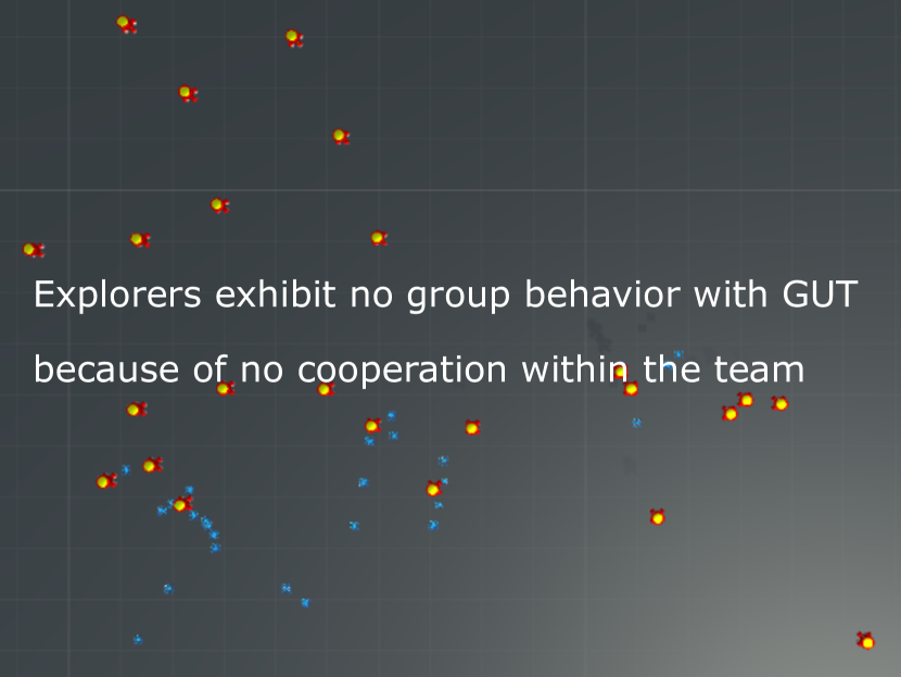
Figure 3. GUT (NC)

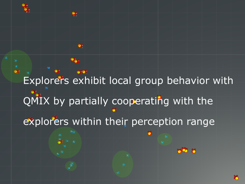
Figure 4. Greedy/QMIX (PC)

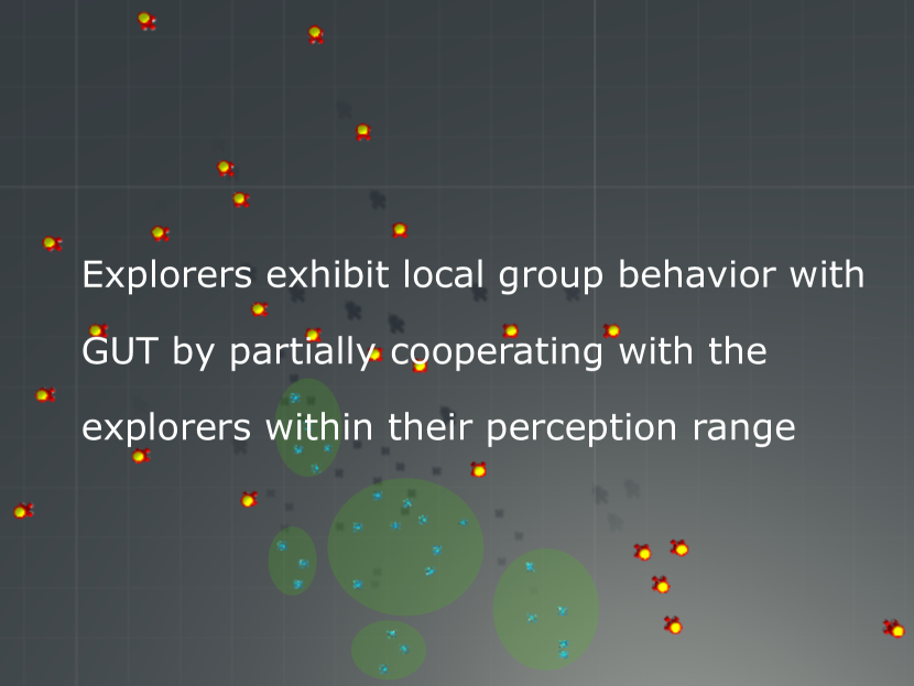
Figure 5. GUT (PC)

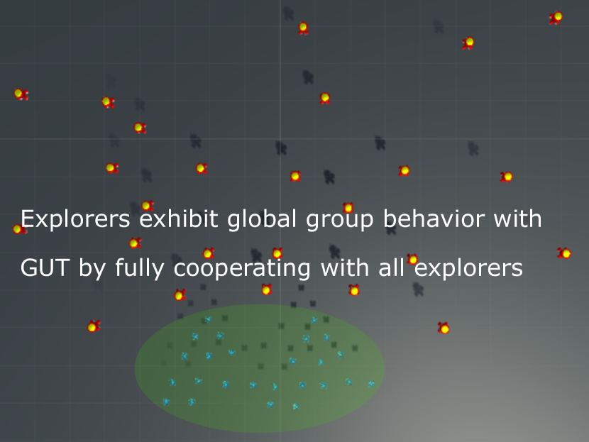
Figure 6. GUT (FC)

4.1. Compared Scenarios and Methods

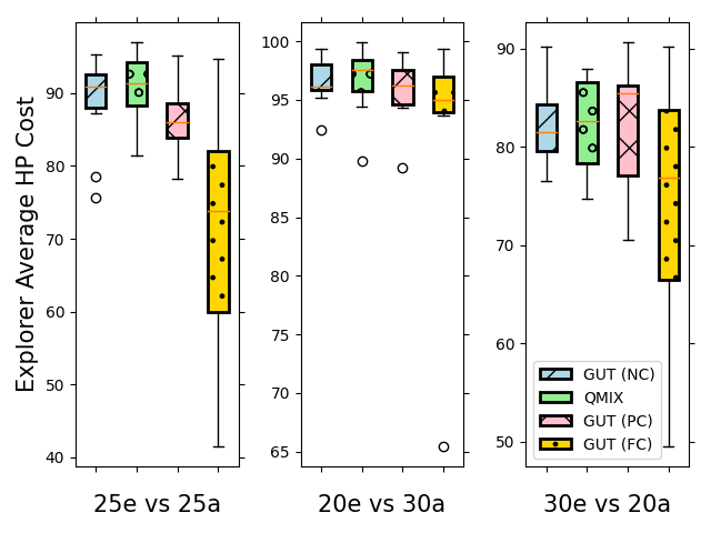
(a) Explorer Average HP Cost

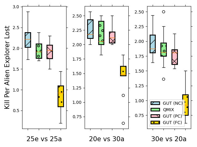
(b) Kill Per Alien - Explorer Lost

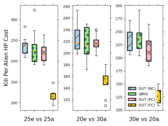
(c) Kill Per Alien - HP Cost

Figure 7. The performance of explorers in interaction experiments with different proportions (e-explorers, a-aliens).

We evaluate GUT from two different scenarios: 1) Interaction Experiments compares the performance of explorers’ cooperative strategies between GUT and Greedy/QMIX methods; 2) Information Prediction demonstrates the GUT when different predictive models are implemented to estimate aliens’ states. Further, we analyze GUT by simulating various cooperation methods, comparing the performance with the state-of-the-art greedy-based approaches - QMIX (Rashid et al., 2018).

1) GUT (NC)

[Noncooperation - Self-interest] In this situation, explorers adopt GUT computing the winning rate based on its perception, but no communication, which means that it does not get the consistency to attack or defend the specific alien (Fig. 6).

2) Greedy/QMIX (PC)

[Partial Cooperation] QMIX is a value-based RL method applied to MAS . It allows each agent to participate in a decentralized execution solely by choosing greedy actions for its rewards. Accordingly, we assume that each explorer can cooperate, communicate, and share information with its observing explorers. Then through calculating the corresponding win rate based on the number of observed explorers and aliens, it chooses to attack or defend the specific hp lowest target (Fig. 6).

3) GUT (PC)

[Partial Cooperation] Here, we consider the same situation as QMIX, but explorers calculate the winning rate with GUT with consistency in strategic decisions (Fig. 6).

4) GUT (FC)

[Full Cooperation - Collective Rationality] In this approach, we assume each explorer work and make decisions with GUT in full communication mode. This enables every group member to achieve consensus on the decisions in a distributed system, prioritizing group’s interest (Fig. 6).

Especially, in partial cooperation, agents cooperate with their neighbors, which they can sense, to work as a team. As shown in Fig. 6, the entire group has been divided into five subgroups, and each subgroup only optimizes its expected return within it. In contrast, all agents work as one group in full cooperation, shown in Fig. 6, and optimize the whole team’ expected return.

Table 4. Winning Rate Results of the Interaction Experiments.

	GUT (NC)	QMIX (PC)	GUT (PC)	GUT (FC)
20e vs 30a	40%	50%	50%	70%
25e vs 25a	90%	100%	100%	100%
30e vs 20a	100%	100%	100%	100%

4.2. Interaction Experiments

In these experiments, the environment is free of obstacles.We consider three different ratios (A/E) between the number of aliens and explorers as follows: 20 explorers vs 30 aliens, 25 explorers vs 25 aliens and 30 explorers vs 20 aliens. For each scenario, we conduct ten simulation trials for each proportion with the same environment setting . In these experiments, the aliens follow a self-interest (noncooperation) random action strategy, while the explorers follow either the GUT or Greedy strategy with different cooperation mentioned in Sec. 4.1.

Results

Fig. 7 presents the performance results in the interaction experiments. We can see that GUT (FC) has the best performance compared with other cases in terms of low HP costs and loss of explorers to win against aliens. Table. 4 shows the winning rate, which also reflects similar results.

Specifically, the GUT (NC), QMIX, and GUT (PC) do not have much difference between in explorer average HP cost results (Fig. 7(a)), but in num. of explorers lost for killing an alien (Fig. 7(b)) and HP cost for killing an alien (Fig. 7(c)), the QMIX and GUT (PC) show some advantage comparing with GUT (NC). The results show that cooperation conduces to decrease the costs and boost the winning rate for more challenging tasks. More importantly, GUT can help agents represent more complex group behaviors and strategies, such as forming various shapes and separating different groups adapting adversarial environments in MAS cooperation. It vastly improves system performance, adaptability, and robustness. Besides, communication plays an essential role in cooperation, such as solving conflicts and getting consistency through negotiation. In GUT (NC) and QMIX, agents only share local information about the number of observing agents for naive attacking or defending behaviors. However, GUT (FC) presents more complex relationships between agents’ cooperation by organizing global communication data.

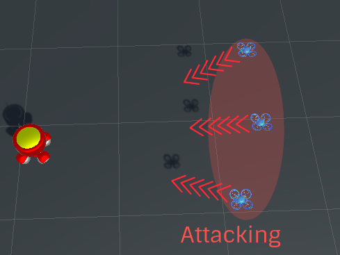
Figure 8. One Alien QMIX

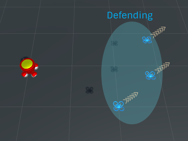
Figure 9. One Alien GUT

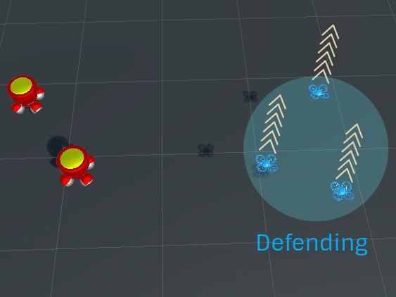
Figure 10. Two Aliens QMIX

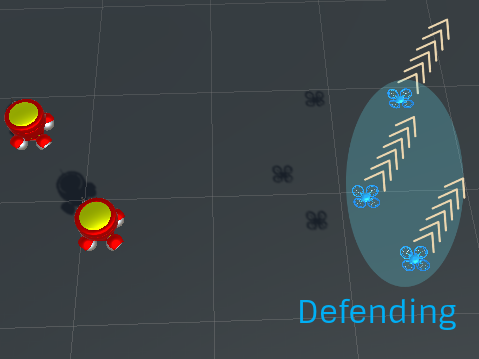
Figure 11. Two Aliens GUT

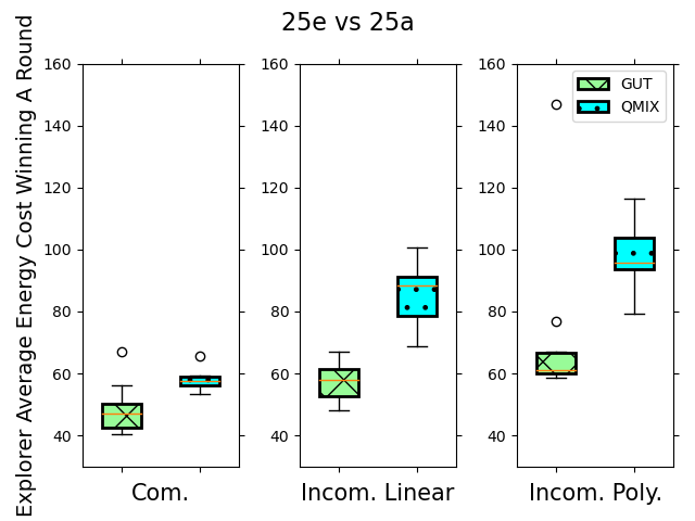
(a) Explorer Average Energy Cost

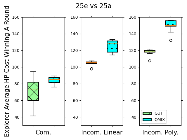
(b) Explorer Average HP (Health) Cost

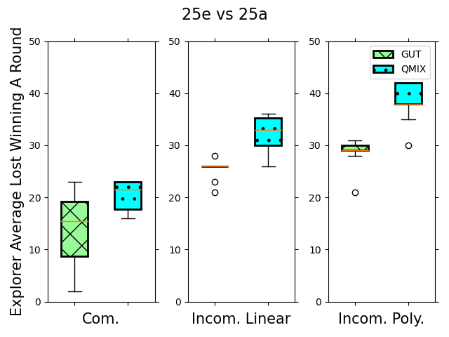
(c) Number of explorers lost per winning round

Figure 12. Explorers’ performance results with different predictive models with obstacles in the environment.

To highlight the difference in how the GUT and Greedy/QMIX approaches work, let us consider an example scenario where an explorer team has only two strategies, attack and defend. For the QMIX approach, selecting attacking or defending relates to the number of the partial group and opponents and their attacking ability directly. However, for the GUT, they need to compute the Nash Equilibrium on all possible strategies both sides can take. The payoff values are calculated based on relative shared information before selecting a suitable strategy. It means that agents might choose a different strategy in the same condition, comparing QMIX and GUT.

For example, in a scenario with one adversary, the greedy method chooses to attack the adversary (Fig. 11), while the GUT chooses to defend against the adversary (Fig. 11). However, in a scenario with two adversaries, QMIX (Fig. 11) and GUT (Fig. 11) have the same strategy reacting to the adversaries. It leads to more costs for the whole system, especially the loss of health (HP), which increases the system’s instability. The two examples explain that instead of choosing greedy actions for group rewards in some scenarios, we need to consider various needs within the team and individual and balance them in a long round. It can improve the sustainability and robustness of the group, especially in uncertain environments.

4.3. Information Prediction

We design two kinds of perceiving models to analyze individual and system performance. 1) In complete information scenario, if an agent can perceive an adversary, it can detect the adversary’s status, such as the unit attacking energy cost and energy level. 2) In incomplete information scenario, an agent can not gain opponents’ state in its observable range.

Assuming that adversary’s unit HP cost HP_uc and average system cost HP_asc can be perceived. Then, we use two prediction models (Linear regressor - Eq. (32) and Polynomial regressor - Eq. (33)) to predict adversaries’ unit attacking energy cost $E_{uc}$ and current energy level $E_{el}$ based on the corresponding HP costs of the adversary.

(32) $$\begin{split}&E_{uc}=HP_{uc}\times\beta_{uc_{0}}+\varepsilon;\\ &E_{el}=100-HP_{asc}\times\beta_{asc_{0}}+\varepsilon.\end{split}$$

(33) $$\begin{split}&E_{uc}=HP_{uc}^{2}\times\beta_{uc_{2}}+HP_{uc}\times\beta_{uc_{1}}+\varepsilon;\\ &E_{el}=100-HP_{asc}^{2}\times\beta_{asc_{2}}-HP_{asc}\times\beta_{asc_{1}}+\varepsilon.\end{split}$$

4.3.1. Environment without obstacles

In this scenario, we consider five proportions of explorers and aliens distributed on the map randomly. For each ratio, we also conduct ten simulation trials with the same experimental setting.

Results

Table 5 shows the results of these experiments. From an agent’s perspective, the Linear Regression model has more accuracy than the Polynomial Regression model, comparing with the result trend of Complete Information (ground truth). From a system perspective, the win rate and the mean energy/HP cost with different predictive models show similar results.

4.3.2. Environment with obstacles

In this scenario, we consider a more complex environment, where there are obstacles (two mountains in the experiment setting) as well as adversaries. Here, the aliens adopt the Greedy/QMIX approach to make their individual decision, while explorers use either QMIX or GUT. We fix the number of explorers (E=25) and aliens (A=25) and conduct ten trials for each predictive model. To implement this scenario, we designed an obstacle avoidance algorithm, which can help agents collectively avoid obstacles by adapting their edge’s trajectory until it finds a suitable route to the goal.

Table 5. System Utility Comparison. Ra: Ratio of Explorers to Aliens, WR: Winning Rate, C${}_{s_{e}/w}$: system average energy cost winning a round, C${}_{s_{hp}/w}$: system average HP cost winning a round.

Ra	Complete Info			Incomplete - Linear Prediction			Incomplete - Poly Prediction
	WR	C${}_{s_{e}/w}$	C${}_{s_{hp}/w}$	WR	C${}_{s_{e}/w}$	C${}_{s_{hp}/w}$	WR	C${}_{s_{e}/w}$	C${}_{s_{hp}/w}$
Environment without obstacles
20:30	70%	1077.37	2649.80	30%	2367.14	6306.90	30%	2726.64	6216.44
20:25	90%	818.63	2027.98	50%	1414.84	3807.23	40%	1375.83	4824.64
25:25	100%	1211.09	1772.00	90%	1432.06	2606.12	80%	1789.15	2949.89
25:20	100%	1414.35	1739.78	100%	1449.07	1960.45	100%	1472.46	2177.52
30:20	100%	1608.18	2241.09	100%	2041.85	2370.76	100%	1961.86	2271.48
Environment with obstacles
25:25	100%	1443.85	2110.91	70%	2144.10	3143.63	60%	2451.37	3742.98

Results

Through the performance results (normalized per explorer) shown in Fig. 12, we notice that due to obstacles (unintentional adversaries) involved, agents’ average HP and energy cost for winning a round increase distinctly. Especially, Fig. 12(c) describes the average number of explorers sacrificed in the game to win in a round as a team against adversaries. The data show that the Linear Regression model presents higher accuracy than the Polynomial model because the current energy and HP calculation models do not involve nonlinear factors. Table. 5 showing the system-level performance results reveal a similar conclusion that obstacles lead to the decrease of the winning rate and more system costs compared to the scenario without obstacles.

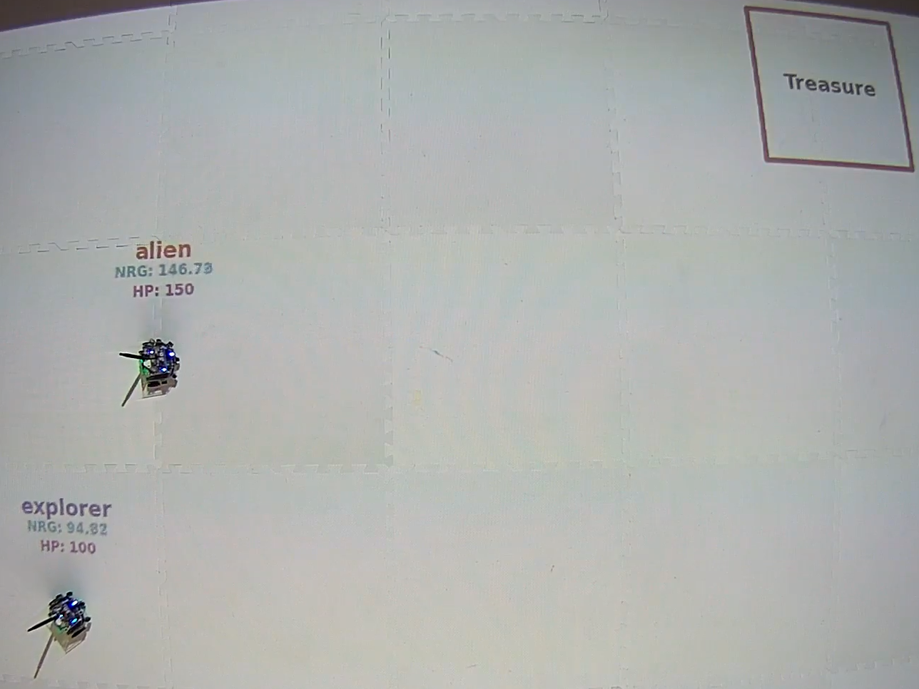
Figure 13. 1 explorer vs 1 alien

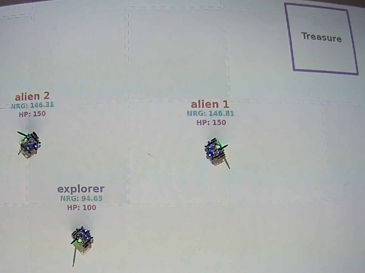
Figure 14. 1 explorer vs 2 aliens

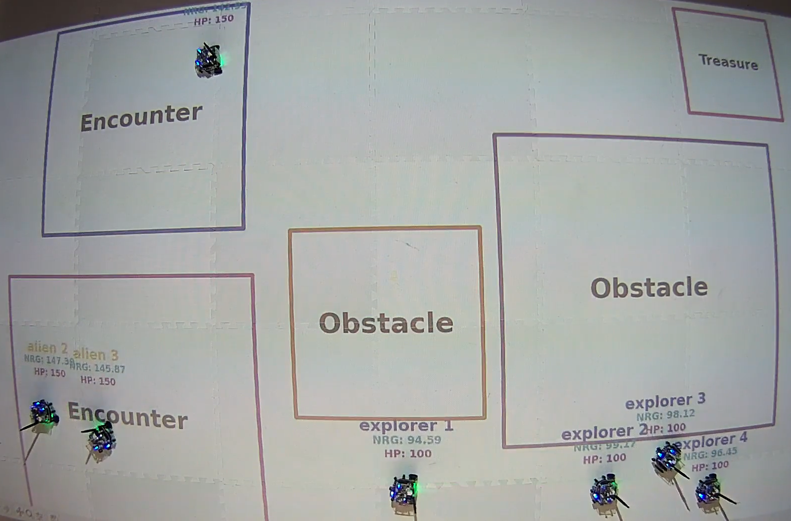
Figure 15. 4 explorers vs 3 aliens

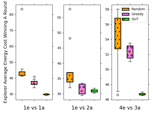
(a) Explorer Average Energy Cost

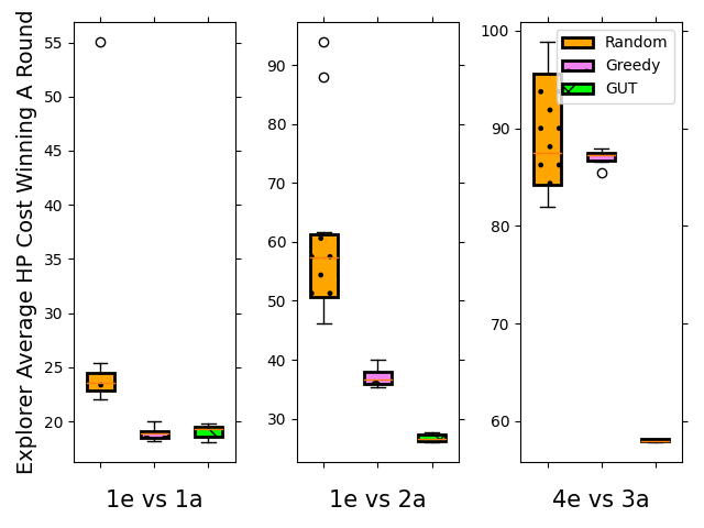
(b) Explorer Average HP Cost

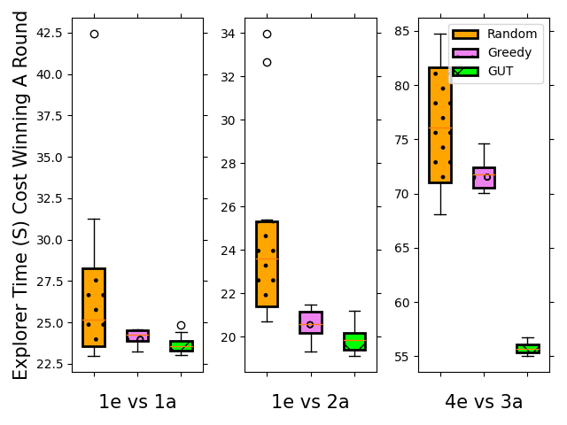
(c) Explorer Time Cost

Figure 16. The Performance Results in the Robotarium Experiments with Different Proportion of the Explore Domain.

5. Robotarium Experiments

To demonstrate the GUT on the multi-robot applications, we implement our method in the Robotarium (Pickem et al., 2017) platform, a remote-accessible multi-robot experiment testbed that supports controlling up to 20 robots simultaneously on a 3.2m $\times$ 2.0m large rectangular area. Each robot has the dimensions 0.11 m $\times$ 0.1 m $\times$ 0.07 m in the testbed. The platform also provides a simulator helping users test their code, which can rapidly prototype their distributed control algorithms and receive feedback about their implementation feasibility before sending them to be executed by the robots on the Robotarium.

In the Robotarium experiments, we consider three different propositions between the number of explorers and aliens in the Explore Game domain. They are one explorer vs. one alien (Fig. 15), one explorer vs. two aliens (Fig. 15), and four explorers vs. three aliens (Fig. 15). To highlight the difference between each experiment, we do not consider any obstacles in the first two scenarios. The third scenario involves (simulated) obstacle regions and two different adversarial regions (Encounters).

Table 6. Level 2 payoff matrix for single explorer.

	$\Delta$Speed	$\Delta$Direction
Follow	$HP_{SF}$	$HP_{DF}$
Retreat	$HP_{SR}$	$HP_{DR}$

Table 7. Level 2 payoff matrix for multiple explorers.

	Triangle	Diamond
Follow	$HP_{TF}$	$HP_{DF}$
Retreat	$HP_{TR}$	$HP_{DR}$

Our Robotarium experiments consider four different strategies (Set $S_{e}$) for the explorer team: attacking and changing direction, attacking and changing speed, defending and changing direction, and defending and changing speed. We decompose this strategy set into two levels for GUT implementation in Robotarium: Level 1 considers deciding attack or defend (Table 3); and Level 2 considers changing direction or speed (Table 7) for a single explorer game while it considers triangle or diamond formation shape (Table 7) for a multiple explorer game. Two different tactics payoff matrices are designed in Level 2 to differentiate the strategies between single-agent and Multi-Agent cooperation.

We compare our GUT approach with two different baseline approaches: 1) Random value selection approach (Eq. (34)), which chooses a strategy from a set $S_{e}$ by maximizing a reward function with two random variables; 2) Greedy algorithm (Vince, 2002) (Eq. (34)), which maximizes the combined utilities of win rate and HP metric together (equivalent to a one-level GUT).

(34) $$\begin{split}&s_{e}^{*}=\mathop{\operatorname*{arg\,max}_{i\in S_{e}}}\mathop{\left[100-c_{1}\cdot s_{i_{1}}\cdot d-c_{2}\cdot s_{i_{2}}\cdot n_{a}\cdot u_{hp}\right]}\\ &s_{e}^{*}=\mathop{\operatorname*{arg\,max}_{i\in S_{e}}}\mathop{\left[W_{i}\cdot HP_{i}\right]}\end{split}$$

We implement each case with real robots in the Robotarium and conduct ten simulation trials (rounds) for each scenario in the Robotarium simulator. We initialize each robot in the same group (explorer or adversary) with equal energy (battery) levels and health points (HP); for example, explorer with 100 points and alien with 150 points in Energy and HP correspondingly. Also, we assumed that every moving step and attack damage cost 0.1% of energy and 0.3% of HP, respectively. Other settings are similar to the previous experiments.

Results and Discussion

Fig. 16 presents the results of the Robotarium experiments. The average costs of energy, HP, and the time taken to complete the mission of explorer are shown in Figs. 16(a), 16(b), and 16(c), respectively. The data shows that in the single explorer cases (scenarios 1e vs. 1a and 1e vs. 2a), both GUT and greedy stand out compared to the random approach, but the GUT is not significantly better than the greedy approach consistently in all the performance metrics. We attribute this to the fact that GUT uses only two levels of action decomposition and therefore does not offer significant advantages compared to the one-level GUT/greedy approach in this simple scenario. However, for the multiple explorer case (scenario 4e vs. 3a), the GUT shows superior performance over other methods in all metrics, demonstrating that the GUT can help MAS organize their behaviors and select a suitable strategy adapting to complex situations. We can get a similar observation from the perspective of the winning rate and the average number of explorers lost from the Table. 8.

Table 8. Performance results in Robotarium experiments.

	Winning Rate			Lost Explorers Per Round/win
	Random	Greedy	GUT	Random	Greedy	GUT
1e vs 1a	100%	100%	100%	-	-	-
1e vs 2a	90%	100%	100%	0.1	-	-
4e vs 3a	50%	90%	100%	2.8	2.0	-

Generally speaking, by demonstrating the Explore domain in the Robotarium, we further proofed that the GUT could help the intelligent agent (robot) rationally analyze different situations in real-time, effectively decompose the high-level strategy into low-level tactics, and reasonably organize groups’ behaviors to adapt to the current scenario. From the system perspective, through applying the GUT, the group can present more complex strategies or behaviors to solve the dynamic changing issues and optimize or sub-optimize the group utilities in MAS cooperation. From the individual agent perspective, GUT reduces the agent’s costs and guarantees sustainable development for each group member, much like human society.

6. Conclusion

We introduce a new Game-theoretic Utility Tree (GUT) for Multi-Agent decision-making in adversarial scenarios and present an example real-time strategy game called Explore Domain. Through extensive numerical simulations, we analyze GUT and compare it against a state-of-the-art cooperative decision-making approach, such as the greedy selection method in QMIX. We verified the effectiveness of GUT through two types of experiments involving interaction and information prediction between the agents. The results showed that the GUT could organize more complex relationships among MAS cooperation, helping the group achieve more challenging tasks with lower costs and higher winning rates. Further, we proofed the effectiveness of the GUT in the real robot application through the implementation of the Explore Domain on the Robotarium. It demonstrated that the GUT could effectively organize Multi-Agent cooperation strategies, enabling a group with fewer advantages to achieve higher performance.

References

- (1)
- Agmon et al. (2011) Noa Agmon, Gal A Kaminka, and Sarit Kraus. 2011. Multi-robot adversarial patrolling: facing a full-knowledge opponent. Journal of Artificial Intelligence Research 42 (2011), 887–916.
- Bakolas and Lee (2021) Efstathios Bakolas and Yoonjae Lee. 2021. Decentralized game-theoretic control for dynamic task allocation problems for multi-agent systems. In 2021 American Control Conference (ACC). IEEE, 3228–3233.
- Browning et al. (2005) Brett Browning, James Bruce, Michael Bowling, and Manuela Veloso. 2005. STP: Skills, tactics, and plays for multi-robot control in adversarial environments. Proceedings of the Institution of Mechanical Engineers, Part I: Journal of Systems and Control Engineering 219, 1 (2005), 33–52.
- Celli and Gatti (2018) Andrea Celli and Nicola Gatti. 2018. Computational results for extensive-form adversarial team games. In Proceedings of the AAAI Conference on Artificial Intelligence, Vol. 32.
- Chung et al. (2011) Timothy H Chung, Geoffrey A Hollinger, and Volkan Isler. 2011. Search and pursuit-evasion in mobile robotics. Autonomous robots 31, 4 (2011), 299.
- Cormen et al. (2009) Thomas H Cormen, Charles E Leiserson, Ronald L Rivest, and Clifford Stein. 2009. Introduction to algorithms. MIT press.
- Daskalakis et al. (2009) Constantinos Daskalakis, Paul W Goldberg, and Christos H Papadimitriou. 2009. The complexity of computing a Nash equilibrium. SIAM J. Comput. 39, 1 (2009), 195–259.
- Jiang and Leyton-Brown (2009) Albert Xin Jiang and Kevin Leyton-Brown. 2009. A Tutorial on the Proof of the Existence of Nash Equilibria. University of British Columbia Technical Report TR-2007-25. pdf 14 (2009).
- Jun and D’Andrea (2003) Myungsoo Jun and Raffaello D’Andrea. 2003. Path planning for unmanned aerial vehicles in uncertain and adversarial environments. In Cooperative control: models, applications and algorithms. Springer, 95–110.
- Kim (2018) Jonghoek Kim. 2018. Multirobot exploration while building power-efficient sensor networks in three dimensions. IEEE transactions on cybernetics 49, 7 (2018), 2771–2778.
- Koller and Friedman (2009) Daphne Koller and Nir Friedman. 2009. Probabilistic graphical models: principles and techniques. MIT press.
- Makkapati and Tsiotras (2019) Venkata Ramana Makkapati and Panagiotis Tsiotras. 2019. Optimal Evading Strategies and Task Allocation in Multi-player Pursuit–Evasion Problems. Dynamic Games and Applications (2019), 1–20.
- McKelvey et al. (2006) Richard D McKelvey, Andrew M McLennan, and Theodore L Turocy. 2006. Gambit: Software tools for game theory. Version 0.2006. 01.20.
- Myerson (2013) Roger B Myerson. 2013. Game theory. Harvard university press.
- Nadarajah and Sundaraj (2013) Sivadev Nadarajah and Kenneth Sundaraj. 2013. A survey on team strategies in robot soccer: team strategies and role description. Artificial Intelligence Review 40, 3 (2013), 271–304.
- Parker (2007) Lynne E Parker. 2007. Distributed Intelligence: Overview of the Field and its Application in Multi-Robot Systems.. In AAAI Fall Symposium: Regarding the Intelligence in Distributed Intelligent Systems. 1–6.
- Pickem et al. (2017) Daniel Pickem et al. 2017. The robotarium: A remotely accessible swarm robotics research testbed. In 2017 IEEE International Conference on Robotics and Automation (ICRA). IEEE, 1699–1706.
- Rashid et al. (2018) Tabish Rashid et al. 2018. QMIX: Monotonic Value Function Factorisation for Deep Multi-Agent Reinforcement Learning. In Proceedings of the 35th International Conference on Machine Learning (Proceedings of Machine Learning Research). PMLR.
- Shen et al. (2004) Jiaying Shen, Xiaoqin Zhang, and Victor Lesser. 2004. Degree of local cooperation and its implication on global utility. In Proceedings of the Third International Joint Conference on Autonomous Agents and Multiagent Systems-Volume 2. IEEE Computer Society, 546–553.
- Sohrabi and Azgomi (2020) Mohammad Karim Sohrabi and Hossein Azgomi. 2020. A survey on the combined use of optimization methods and game theory. Archives of Computational Methods in Engineering 27, 1 (2020), 59–80.
- Stone and Veloso (2000) Peter Stone and Manuela Veloso. 2000. Multiagent systems: A survey from a machine learning perspective. Autonomous Robots 8, 3 (2000), 345–383.
- Vince (2002) Andrew Vince. 2002. A framework for the greedy algorithm. Discrete Applied Mathematics 121, 1-3 (2002), 247–260.
- Vinyals et al. (2019) Oriol Vinyals et al. 2019. Grandmaster level in StarCraft II using multi-agent reinforcement learning. Nature 575, 7782 (2019), 350–354.
- von Stengel and Koller (1997) Bernhard von Stengel and Daphne Koller. 1997. Team-maxmin equilibria. Games and Economic Behavior 21, 1-2 (1997), 309–321.
- Wooldridge (2009) Michael Wooldridge. 2009. An introduction to multiagent systems. John Wiley & Sons.
- Yang (2022) Qin Yang. 2022. Self-Adaptive Swarm System. Ph.D. Dissertation. University of Georgia.
- Yang et al. (2019) Qin Yang, Zhiwei Luo, Wenzhan Song, and Ramviyas Parasuraman. 2019. Self-reactive planning of multi-robots with dynamic task assignments. In 2019 International Symposium on Multi-Robot and Multi-Agent Systems (MRS). IEEE, 89–91.
- Yang and Parasuraman (2020a) Qin Yang and Ramviyas Parasuraman. 2020a. Hierarchical needs based self-adaptive framework for cooperative multi-robot system. In 2020 IEEE International Conference on Systems, Man, and Cybernetics (SMC). IEEE, 2991–2998.
- Yang and Parasuraman (2020b) Qin Yang and Ramviyas Parasuraman. 2020b. Needs-driven heterogeneous multi-robot cooperation in rescue missions. In IEEE International Symposium on Safety, Security, and Rescue Robotics (SSRR). IEEE, 252–259.
- Yang and Parasuraman (2021) Qin Yang and Ramviyas Parasuraman. 2021. How Can Robots Trust Each Other For Better Cooperation? A Relative Needs Entropy Based Robot-Robot Trust Assessment Model. In 2021 IEEE International Conference on Systems, Man, and Cybernetics (SMC). IEEE, 2656–2663.
- Yehoshua and Agmon (2015) Roi Yehoshua and Noa Agmon. 2015. Adversarial modeling in the robotic coverage problem. In Proceedings of the 2015 International Conference on Autonomous Agents and Multiagent Systems. International Foundation for Autonomous Agents and Multiagent Systems, 891–899.
- Zhang et al. (2014) Jian-liang Zhang, Dong-lian Qi, and Miao Yu. 2014. A game theoretic approach for the distributed control of multi-agent systems under directed and time-varying topology. International Journal of Control, Automation and Systems 12, 4 (2014), 749–758.