Targeted Adversarial Attacks on Wind Power Forecasts

Abstract

In recent years, researchers proposed a variety of deep learning models for wind power forecasting. These models predict the wind power generation of wind farms or entire regions more accurately than traditional machine learning algorithms or physical models. However, latest research has shown that deep learning models can often be manipulated by adversarial attacks. Since wind power forecasts are essential for the stability of modern power systems, it is important to protect them from this threat.
In this work, we investigate the vulnerability of two different forecasting models to targeted, semi-targeted, and untargeted adversarial attacks. We consider a Long Short-Term Memory (LSTM) network for predicting the power generation of individual wind farms and a Convolutional Neural Network (CNN) for forecasting the wind power generation throughout Germany. Moreover, we propose the Total Adversarial Robustness Score (TARS), an evaluation metric for quantifying the robustness of regression models to targeted and semi-targeted adversarial attacks. It assesses the impact of attacks on the model’s performance, as well as the extent to which the attacker’s goal was achieved, by assigning a score between 0 (very vulnerable) and 1 (very robust). In our experiments, the LSTM forecasting model was fairly robust and achieved a TARS value of over 0.78 for all adversarial attacks investigated. The CNN forecasting model only achieved TARS values below 0.10 when trained ordinarily, and was thus very vulnerable. Yet, its robustness could be significantly improved by adversarial training, which always resulted in a TARS above 0.46.

Keywords Adversarial Machine Learning  $\cdot$ Windpower Forecasting  $\cdot$ Robustness Evaluation  $\cdot$ Adversarial Training  $\cdot$ Time Series Forecasting  $\cdot$ Deep Learning

1 Introduction

Renewable energy forecasting has a significant impact on the planning, management, and operation of power systems [1]. Grid operators and power plants require accurate forecasts of renewable energy output to ensure grid reliability and permanency, and to reduce the risks and costs of energy markets and power systems [2]. Over the past few years, the share of renewable energies in the electricity mix has risen steadily. For example, the total installed wind energy capacity in Germany increased from 26.9 gigawatts in 2010 to 63.9 gigawatts in 2021 [3]. Moreover, wind energy already covered about 20 percent of the German gross electricity consumption in 2021, making it the most important energy carrier in the German electricity mix. This development poses a challenge for energy providers. Wind power generation is difficult to predict due to the randomness, volatility, and intermittency of wind. Improving the accuracy of wind power forecasts is therefore of high importance.
In recent years, Deep Learning (DL) methods have proven to be particularly feasible and effective for accurate renewable energy forecasting [1, 2, 4]. Nevertheless, power systems are a critical infrastructure that can be targeted by criminal, terrorist, or military attacks. Hence, not only the accuracy of wind power forecasts is relevant, but also their attack resistance. Latest research has shown that DL methods are often vulnerable to adversarial attacks [5, 6]. The use of DL thus poses dangers and opens up new attack opportunities for assailants. Adversarial attacks slightly perturb the input data of Machine Learning (ML) models to falsify their predictions. In particular, DL algorithms that obtain input data from safety-critical interfaces are exposed to this threat. Wind power forecasting models often use satellite imagery or weather forecasts as input features. Such data frequently comes from publicly available data sources which can be corrupted by hackers. Even data sources that are not public can become the target of attacks. For example, there is a risk that energy data markets [7] will be abused by attackers in the future. Attackers could use these markets to inject tampered data into an ML application and thereby manipulate its predictions. If such manipulations remain undetected and if forecasting models are not adequately protected, the consequences could be fatal. Attacks on wind power forecasts could compromise forecast quality, resulting in high costs for energy consumers and energy providers. Even worse, attackers could also manipulate the forecasts to gain economic advantages or destabilize energy systems.

Consequently, there is a growing interest among researchers to study the effects of adversarial attacks in the context of time series data. In particular, the vulnerability of DL methods for time series classification has been studied by various researchers [8, 9, 10]. They considered adversarial attacks such as the Fast Gradient Sign Method [6] and the Basic Iterative Method [11] to cause misclassification of time series data. More advanced techniques such as the Adversarial Transformation Network [12, 13] have also been proposed for this purpose. However, adversarial attacks on ML algorithms are also highly relevant for regression tasks such as time series forecasting [14]. With respect to DL approaches, [15] examined the impact of adversarial attacks on regression neural networks and proposed a stability-inducing, regularization-based defense against these attacks. Nevertheless, adversarial attacks for regression tasks still require additional research, as the number of contributions on this topic is yet relatively limited.
With the rising adoption of DL in the power industry, the analysis and detection of adversarial attacks is becoming a growing concern. Since energy systems are critical infrastructures, the security of DL algorithms in this domain is of particular importance. According to [16], the DL models deployed in this field can become targets of attacks across the entire value chain. In this regard, an important topic of interest is the protection of grid infrastructures and smart grids against adversarial attacks. The survey of [17] shows that various papers related to false data injection attacks have already been published in this sector. There also exists research that investigates the threat of adversarial attacks designed to fool anomaly detection methods [18, 19]. Other papers cover grid-related topics such as utilizing adversarial attacks for the purpose of energy theft in energy management systems [20] or attacks on event cause analysis [21]. Another important research direction in the energy domain are adversarial attacks on power forecasts. Here, [22] have shown that the prediction accuracy of load flow forecasts can be degraded by stealthy adversarial attacks. Further, [23] have analyzed how load flow forecasts can be biased in a direction advantageous to the attacker. Still other researchers have focused on attacks against renewables. For instance, [24] studied the impact of untargeted adversarial attacks on solar power forecasts.
In this work, the focus is on wind power forecasting, due to its rising importance in power systems. Recently, DL models have been increasingly proposed by researchers for this task [2, 25]. However, very little research has been done on the robustness of these models to adversarial attacks. A notable contribution was made by [26], who approached the problem of false data injection attacks from a technical point of view. In doing so, they examined the impact of untargeted adversarial attacks on a variety of regression models, including support vector machines, fully connected neural networks, and quantile regression neural networks. In contrast to previous studies, the focus of this work is to investigate targeted adversarial attacks on DL models for wind power forecasting. 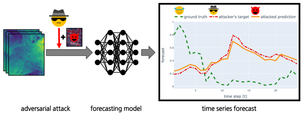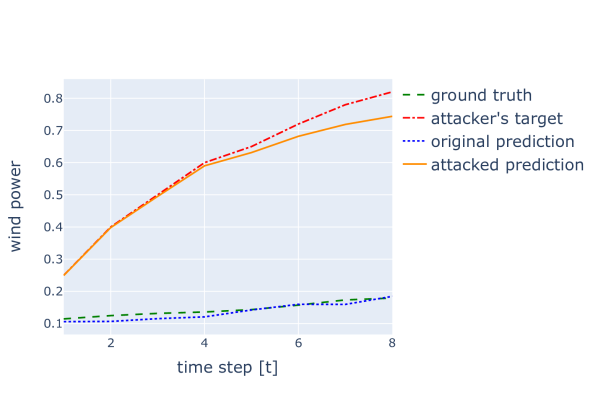The goal of targeted adversarial attacks is to manipulate the forecasting model in such a way that the predicted values follow a specific forecast pattern desired by the attacker, see Fig. 1.
As discussed previously, only untargeted and semi-targeted attacks on DL-based forecasting models have been studied so far. In the case of wind power forecasts, however, targeted adversarial attacks pose a much greater threat. Such attacks give assailants the opportunity to specifically influence forecast behavior. Thus, they are able to affect energy markets or disrupt grid operations. Especially in regression tasks, evaluating the success of targeted adversarial attacks is non-trivial. Therefore, it is important to have appropriate evaluation metrics for assessing the robustness of models to such attacks. In this work, we address these problems and offer the following contributions:

1. We propose a taxonomy for adversarial attacks in the regression setting that categorizes them into untargeted, semi-targeted, and targeted attacks.

2. We present an evaluation metric for assessing the robustness of regression models to targeted and semi-targeted adversarial attacks. This evaluation metric measures not only the impact of the attacks on the performance of the model, but also the extent to which the attacker’s goal was achieved.

3. We investigate the robustness of two different DL models for wind power forecasting, each with its own use case. We find that CNN models for predicting the wind power generation throughout Germany based on wind speed forecasts in the form of weather maps are very susceptible to adversarial attacks, whereas LSTM models for predicting the power generation of wind farms based on wind speed forecasts in the form of time series are fairly robust.

4. We examine the effects of adversarial training and show that it significantly increases the robustness of the CNN forecasting model, while having only a small effect on the robustness of the LSTM forecasting model in the respective applications.

Figure 1: Illustration of a targeted adversarial attack on a time series forecasting model. The adversary manipulates the input data by adding a small perturbation. This perturbation causes the model’s prediction (solid) to no longer approximate the ground truth (dashed), but to follow a particular forecast pattern (dash-dotted) defined by the attacker

This paper is organized as follows. In Section 2, we present the underlying methodology behind adversarial attacks and adversarial training. Moreover, an evaluation metric for quantifying the adversarial robustness of regression models is proposed. Next, two different DL-based wind power forecasting models are investigated in terms of their robustness to adversarial attacks. First, the experimental setup is presented in Section 3. Subsequently, the results of the study are presented in Section 4. In Section 5, a discussion of the results follows and several directions for future work are pointed out. Finally, we conclude with a summary of this contribution in Section 6.

2 Methodology

2.1 Adversarial attacks

Adversarial attacks refer to attacks on ML algorithms that perturb the input data in order to manipulate the model’s prediction. In the process, the attacker modifies the input data slightly and carefully, so that the perturbations remain undetected by humans and anomaly detection methods. The techniques for generating adversarial attacks can be taxonomically categorized according to the attacker’s goal and the prior knowledge of the attacker [27]. Whereas white-box adversarial attacks require complete knowledge about the model architecture and the trained model parameters, gray-box methods assume only limited knowledge of the attacker, e.g., about confidence levels of the model. Black-box methods, on the other hand, suppose that the attacker has no knowledge about the underlying model. However, it is commonly assumed that the attacker is able to communicate with the model.
Regarding the attacker’s goal, a distinction is made between untargeted and targeted attacks in classification tasks. The goal of targeted attacks is to fool the model into classifying the input as a particular class desired by the adversary. In contrast, untargeted attacks simply aim for a misclassification of the perturbed data. The exact class predicted by the model is not important. For regression tasks, though, the output of ML algorithms is not categorical, but represents continuous variables. Thus, this categorization of adversarial attacks cannot be simply transferred to regression problems.

2.1.1 Goals of adversarial attacks in regression tasks

As contribution (C1), we propose to taxonomically divide the attacker’s goal into three categories in the regression setting: untargeted attacks, semi-targeted attacks, and targeted attacks. Untargeted attacks attempt to perturb an input data point $x\in\mathbb{R}^{d}$ in such a way that the prediction quality of a model $f_{\theta}$, with parameters $\theta\in\mathbb{R}^{p}$, is degraded to the maximum in terms of a loss function $\mathcal{L}$. The objective that the attacker wants to optimize is as follows:

$$\max_{\delta\in\mathcal{S}}\mathcal{L}\left(f_{\theta}(x+\delta),y\right)$$ (1)

Here, $y\in\mathbb{R}^{n}$ is the ground truth value associated with the input data point $x$. The perturbation added to $x$ is denoted by $\delta$, and $\mathcal{S}\subseteq\mathbb{R}^{d}$ represents the set of allowed perturbations. An example of an untargeted adversarial attack on a univariate time series forecast is shown in Figure 2.

Figure 2: Example of an untargeted adversarial attack. While the original prediction (dotted) approximates the ground truth (dashed) very well, the attacked prediction (solid) deviates strongly from the ground truth

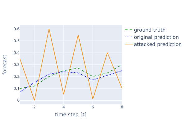
In the case of untargeted attacks, the attacker has no control over the magnitude of the degradation. Thus, he risks that the attack will result in an unrealistic prediction that can easily be detected as erroneous.
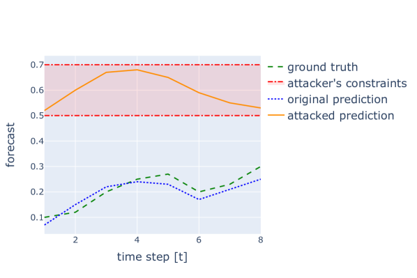
To avoid this, attackers also have the option of launching semi-targeted attacks on regression models. We define semi-targeted attacks as perturbations that cause the model’s predictions to fall within certain boundaries. These boundaries are specified by the attacker. Thus, the perturbations aim at degrading the model’s performance, while satisfying certain constraints:

$$\begin{split}\max_{\delta\in\mathcal{S}}\quad&\mathcal{L}\left(f_{\theta}(x+\delta),y\right)\\ \text{s.t.}\quad&C_{i}\left(f_{\theta}(x+\delta)\right)\leq 0\quad\text{for }i=1,\dots,k\\ &C_{j}\left(f_{\theta}(x+\delta)\right)=0\quad\text{for }j=1,\dots,l\end{split}$$ (2)

Here, the inequality constraints $C_{i}$ and the equality constraints $C_{j}$ describe the attacker’s desired restrictions on the behavior of the manipulated prediction $f_{\theta}(x+\delta)$. For example, the attacker may attempt to degrade the prediction quality only to a certain degree so that the degradation remains inconspicuous. Another example are perturbations that cause the prediction to be distorted as much as possible in a certain direction, e.g., to either increase or decrease the predicted values, as was studied by [23]. In this work, we study semi-targeted adversarial attacks with lower and upper bound constraints. Here, the attacker specifies a lower bound $a\in\mathbb{R}^{n}$ and an upper bound $b\in\mathbb{R}^{n}$. The attacker then attempts to perturb the input data such that the attacked prediction $\hat{y}_{adv}=f_{\theta}(x+\delta)$ falls within the region enclosed by the lower and upper bound, i.e., $a_{i}\leq\hat{y}_{adv,i}\leq b_{i}$ holds for all $i=1,\dots,n$. In the example in Figure 3, the constraints require the prediction $\hat{y}_{adv}$ to only take values between 0.5 and 0.7.

Figure 3: Example of a semi-targeted adversarial attack. While the original prediction (dotted) approximates the ground truth (dashed) very well, the attacked prediction (solid) lies in the area defined by the attacker’s constraints (dash-dotted)

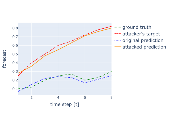
Finally, regression models can also be manipulated by attackers in a targeted fashion. Targeted attacks try to perturb the input data in such a way that the model’s prediction comes as close as possible to an adversarial target $y_{adv}\in\mathbb{R}^{n}$. Thus, the attacker aims for the following optimization objective:

$$\min_{\delta\in\mathcal{S}}\mathcal{L}\left(f_{\theta}(x+\delta),y_{adv}\right)$$ (3)

Depending on the application, different target values may be relevant for the attacker. For instance, an attacker could try to manipulate wind power forecasts in order to influence energy markets and gain economic advantages. An example of a targeted adversarial attack is shown in Figure 4.

Figure 4: Example of a targeted adversarial attack. While the original prediction (dotted) almost matches the ground truth (dashed), the attacked prediction (solid) approximates the attacker’s target (dash-dotted)

In this paper, two methods for generating adversarial attacks are considered. The focus is on untargeted, semi-targeted, and targeted adversarial attacks using the Projected Gradient Descent (PGD) attack. In addition, we also examine untargeted adversarial noise attacks, which are rather weak attacks but serve as a baseline. The two methods are described below.

2.1.2 Adversarial noise attack

A very simple form of untargeted adversarial attacks are adversarial noise attacks, which were originally introduced by [28]. Noise attacks are applicable to both classification tasks and regression tasks. They perturb the input data by adding random noise, commonly Gaussian noise or uniform noise. In the process, the perturbation is normalized and rescaled to the desired size, e.g., with respect to the $L_{\infty}$ norm. In addition, the perturbed samples need to be clipped afterwards so that all values are within the valid lower and upper bounds of the input data [29]. Noise attacks require no prior knowledge of the model and thus represent black-box attacks. In order to increase the success rate of the attack, repeated noise attacks can be used. Here, noise is repeatedly sampled, thus generating several candidate noise terms for the attack. Then the effects of the different noise terms on the model’s performance are evaluated. Finally, the noise term that most degrades the model’s performance is selected as the perturbation.

2.1.3 Projected Gradient Descent (PGD) attack

According to [30], by far the most powerful attack algorithms are those that use gradient-based optimization. They extract a significant amount of information from the model by using the gradients of a loss function to generate adversarial attacks. One such optimization-based attack commonly used in the literature is PGD, which was originally proposed by [31]. PGD attempts to iteratively improve the perturbation of an input, while always ensuring that the magnitude of the perturbation is within a given boundary. To do this, PGD exploits the model gradients between the input and an adversarial loss function. Thus, it is a white-box attack and applicable for untargeted, semi-targeted as well as targeted attacks.
In the case of untargeted attacks, PGD attempts to maximize the deviation between the model’s prediction and the ground truth [11]:

$$x_{adv}^{\left(0\right)}=x,\quad x_{adv}^{\left(t+1\right)}=\operatorname{Clip}_{x,\epsilon}\left\{x_{adv}^{\left(t\right)}+\alpha\text{ sign}\left(\nabla_{x_{adv}^{\left(t\right)}}\mathcal{L}\left(f_{\theta}\left(x_{adv}^{\left(t\right)}\right),y\right)\right)\right\}$$ (4)

On the other hand, in targeted attacks, PGD tries to minimize the mismatch between the model’s prediction and the attacker’s target [11]:

$$x_{adv}^{\left(0\right)}=x,\quad x_{adv}^{\left(t+1\right)}=\operatorname{Clip}_{x,\epsilon}\left\{x_{adv}^{\left(t\right)}-\alpha\text{ sign}\left(\nabla_{x_{adv}^{\left(t\right)}}\mathcal{L}\left(f_{\theta}\left(x_{adv}^{\left(t\right)}\right),y_{adv}\right)\right)\right\}$$ (5)

Here $\alpha$ is the update size per step and $x_{adv}^{\left(t\right)}$ denotes the perturbed input after the $t^{th}$ optimization step. Feature-wise clipping of the perturbed input using the $\operatorname{Clip}_{x,\epsilon}$ function ensures that the result is in the $\epsilon$-neighborhood of the original input $x$, with respect to the $L_{\infty}$ norm. The parameter $\epsilon$ corresponds to the maximum perturbation magnitude specified by the attacker. It should be noted that [31] proposed to add a random initialization to this algorithm. However, in the following experiments we always use PGD without a random initialization, since it did not have a significant effect on the results in preliminary tests.
For applying PGD to semi-targeted attacks, we propose to add a weighted penalty term to the loss function, which penalizes the violation of the attacker’s constraints. In the case of semi-targeted attacks with lower and upper bound constraints, PGD then attempts to maximize the mismatch between the model’s prediction and the ground truth, while at the same time minimizing the deviation between the prediction and the area enclosed by the lower and upper bounds:

$$\begin{split}&x_{adv}^{\left(0\right)}=x,\\ &x_{adv}^{\left(t+1\right)}=\operatorname{Clip}_{x,\epsilon}\left\{x_{adv}^{\left(t\right)}+\alpha\text{ sign}\left(\nabla_{x_{adv}^{\left(t\right)}}\mathcal{L}_{\lambda}\left(f_{\theta}\left(x_{adv}^{\left(t\right)}\right),y,a,b\right)\right)\right\},\\ &\mathcal{L}_{\lambda}\left(f_{\theta}\left(x_{adv}^{\left(t\right)}\right),y,a,b\right)=\mathcal{L}\left(f_{\theta}\left(x_{adv}^{\left(t\right)}\right),y\right)-\lambda\cdot\mathcal{L}_{[a,b]}\left(f_{\theta}\left(x_{adv}^{\left(t\right)}\right)\right)\end{split}$$ (6)

Here, $\mathcal{L}_{[a,b]}\left(f_{\theta}\left(x_{adv}^{\left(t\right)}\right)\right)$ is a loss function that serves as the penalty term. It measures the degree of deviation between the prediction and the area enclosed by the lower bound $a$ and the upper bound $b$. The parameter $\lambda$ is the corresponding penalty weight, which was always chosen as 1000 in this work.

2.2 Adversarial training

Several techniques exist to protect ML algorithms from adversarial attacks [32, 27, 33]. For example, perturbed data points can be identified and eliminated at an early stage using detection methods [34]. Another approach is to increase a model’s robustness. A robust model is characterized by the fact that it is stable to small perturbations of its inputs [5]. In a regression setting, this means that minor changes in the input do not lead to significant changes in the model’s prediction. A commonly used technique in the literature is to increase the robustness of a model by adversarial training [6]. During adversarial training, the model is trained on perturbed training data. Thus, it automatically becomes more robust to the type of adversarial attacks that were used to generate the perturbations in the training phase. In each training iteration, the perturbed data points are newly generated from the original training data. This ensures that the perturbations are specifically tailored to the model weights of each training iteration. Then the model weights $\theta\in\mathbb{R}^{p}$ are selected by solving the following optimization problem [31]:

$$\min_{\theta}\\ \ \mathbb{E}_{\left(x,y\right)\sim\mathcal{D}}\left[\max_{\delta\in\mathcal{S}}\mathcal{L}\left(f_{\theta}\left(x+\delta\right),y\right)\right]$$ (7)

Here, $\left(x,y\right)\sim\mathcal{D}$ represents training data sampled from the underlying data distribution $\mathcal{D}$. The inner maximization problem is to find the worst-case perturbations for the given model weights, which can be approximately solved by generating adversarial attacks with the PGD attack [31]. On the other hand, the outer minimization consists in training a model that is robust to these worst-case perturbations. This can be solved by the standard training procedure.

2.3 Adversarial robustness scores

In order to evaluate the security of DL models, it is essential to quantify their robustness to adversarial attacks. In classification tasks, the success of an attack can be measured quite easily using the model accuracy or the attack success rate [30]. However, assessing the robustness of regression models is non-trivial, especially in the case of targeted and semi-targeted attacks. Therefore, as contribution (C2), we present below an evaluation metric for quantifying the robustness of regression models to targeted adversarial attacks and semi-targeted adversarial attacks with lower and upper bound constraints. From the attacker’s perspective, the success of a targeted attack can be measured by the deviation between the model’s prediction and the adversarial target. In the case of semi-targeted attacks, it is important for the attacker that the prediction satisfies his constraints. But from the victim’s point of view, this does not cover all possible harms. An attack may be unsuccessful for the attacker because the model’s prediction is still far from the adversarial target or does not satisfy the attacker’s constraints. But if the attack significantly degrades the model’s performance, it still has a considerable lack of robustness. Therefore, we propose an evaluation metric to quantify the robustness of regression models specifically for targeted and semi-targeted attacks.
In the following, we use the Root Mean Square Error (RMSE) to measure the deviation between a model’s prediction $\hat{y}=f_{\theta}\left(x\right)\in\mathbb{R}^{n}$ and the associated ground truth $y\in\mathbb{R}^{n}$:

$$\operatorname{RMSE}\left(\hat{y},y\right)=\left(\frac{1}{n}\sum_{i=1}^{n}\left(\hat{y}_{i}-y_{i}\right)^{2}\right)^{\frac{1}{2}}$$ (8)

The RMSE has the benefit of penalizing large errors more. However, it is possible to replace the RMSE in the scores defined below (DRS, PRS, and TARS) with any other non-negative cost function $\mathcal{L}$. For example, the Mean Square Error (MSE) or Mean Absolute Error (MAE) are also very common cost functions for regression problems.
To quantify the extent to which a prediction $\hat{y}\in\mathbb{R}^{n}$ satisfies the lower and upper bound constraints of a semi-targeted attack, we define the following variation of the RMSE, the Bounded Root Mean Square Error (BRMSE):

$$\operatorname{BRMSE}_{[a,b]}\left(\hat{y}\right)=\left(\frac{1}{n}\sum_{i=1}^{n}\left(\chi_{\{\hat{y}_{i}<a_{i}\}}\cdot\left(\hat{y}_{i}-a_{i}\right)^{2}+\chi_{\{b_{i}<\hat{y}_{i}\}}\cdot\left(\hat{y}_{i}-b_{i}\right)^{2}\right)\right)^{\frac{1}{2}}$$ (9)

Here $a\in\mathbb{R}^{n}$ denotes the lower bound, $b\in\mathbb{R}^{n}$ the upper bound and $\chi$ the indicator function. If a prediction $\hat{y}$ satisfies the constraints, i.e., if $a_{i}\leq\hat{y}_{i}\leq b_{i}$ holds for all $i=1,\dots,n$, then the $\operatorname{BRMSE}_{[a,b]}$ is zero. If an element $\hat{y}_{i}$ of the prediction is below the lower bound, i.e. if $\hat{y}_{i}<a_{i}$ holds, the $\operatorname{BRMSE}_{[a,b]}$ accounts only for the deviation between $\hat{y}_{i}$ and $a_{i}$. On the other hand, if an element $\hat{y}_{i}$ is above the upper bound, i.e. if $\hat{y}_{i}>b_{i}$ holds, the $\operatorname{BRMSE}_{[a,b]}$ only considers the deviation between $\hat{y}_{i}$ and $b_{i}$.
The proposed score for evaluating the robustness to targeted and semi-targeted attacks is composed of two subscores. These subscores respectively measure the robustness of the model’s performance and its robustness to prediction deformations. The scores are described in more detail below.

2.3.1 Performance robustness

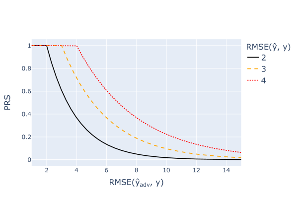
The first score is the Performance Robustness Score (PRS). The PRS measures how severely a model’s performance deteriorates relative to its original performance when under attack:

$$\operatorname{PRS}\left(\hat{y},\hat{y}_{adv},y\right)=\min\left(\exp\left(1-\frac{\operatorname{RMSE}\left(\hat{y}_{adv},y\right)}{\operatorname{RMSE}\left(\hat{y},y\right)+\gamma}\right),1\right)$$ (10)

Here, $\gamma$ is a small constant value to avoid dividing by zero. In the following we always select $\gamma=1\cdot 10^{-10}$. The PRS ranges from 0 to 1. If the deviation between the model’s prediction and the ground truth remains unchanged during the attack or even decreases, the attack has no negative impact on the model’s performance. In this case, the performance is considered robust to the attack and the PRS takes the value 1. However, if $\operatorname{RMSE}\left(\hat{y}_{adv},y\right)$ increases relative to $\operatorname{RMSE}\left(\hat{y},y\right)$, the PRS converges to zero and the performance robustness decreases exponentially, see Fig. 10 in Appendix A.

2.3.2 Deformation robustness

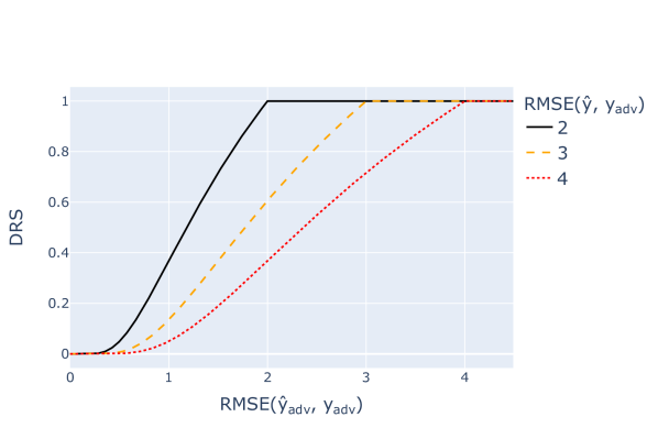
We define the Deformation Robustness Score (DRS) to quantify the success of an attacker in case of targeted and semi-targeted attacks. For targeted attacks, the DRS measures how close a model’s prediction moves towards the adversarial target due to an attack:

$$\operatorname{DRS}\left(\hat{y},\hat{y}_{adv},y_{adv}\right)=\min\left(\exp\left(1-\frac{\operatorname{RMSE}\left(\hat{y},y_{adv}\right)}{\operatorname{RMSE}\left(\hat{y}_{adv},y_{adv}\right)+\gamma}\right),1\right)$$ (11)

The DRS also ranges from 0 to 1. If the DRS is equal to 1, the attack has failed from the attacker’s point of view. This is the case if the model’s prediction has remained unchanged or the deviation between the prediction and the adversarial target has increased as a result of the attack. However, if $\operatorname{RMSE}\left(\hat{y}_{adv},y_{adv}\right)$ decreases relative to $\operatorname{RMSE}\left(\hat{y},y_{adv}\right)$, the DRS converges to zero and the deformation robustness drops exponentially, see Fig. 11 in Appendix A.
Analogously, the DRS can also be defined for semi-targeted attacks with lower and upper bound constraints:

$$\operatorname{DRS}\left(\hat{y},\hat{y}_{adv},a,b\right)=\min\left(\exp\left(1-\frac{\operatorname{BRMSE}_{[a,b]}\left(\hat{y}\right)}{\operatorname{BRMSE}_{[a,b]}\left(\hat{y}_{adv}\right)+\gamma}\right),1\right)$$ (12)

Here, the DRS measures the extent to which the deviation between the model’s prediction and the area enclosed by the lower and upper bound has decreased as a result of the attack.

2.3.3 Total adversarial robustness

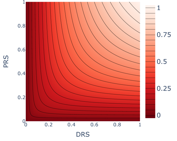
Neither the PRS nor the DRS individually provide a thorough assessment of a regression model’s robustness to targeted or semi-targeted attacks. While the PRS only captures the impact of an attack on the model’s performance, the DRS solely measures how the attack affected the deviation between the model’s prediction and the attacker’s target or the attacker’s constraints. From the victim’s perspective, a model is only considered robust if it has both a high PRS and a high DRS. We therefore define the TARS, which combines the PRS and the DRS into one score. Thus, the TARS provides a comprehensive measure of a model’s robustness:

$$\operatorname{TARS}_{\beta}=\left(1+\beta^{2}\right)\frac{\operatorname{PRS}\cdot\operatorname{DRS}}{\left(\beta^{2}\cdot\operatorname{PRS}\right)+\operatorname{DRS}}$$ (13)

Note that the TARS is inspired by the $F_{\beta}$ score and uses a parameter $\beta\in\mathbb{R}^{+}$. In the case $\beta=1$, the TARS is the harmonic mean between DRS and PRS. Depending on the application, $\beta$ can be adjusted such that the DRS is considered to be $\beta$ times as important as the PRS. Thus, for $\beta>1$, deformation robustness is weighted higher, whereas for $\beta<1$, performance robustness is given more weight. Compared to weighted arithmetic averaging, the TARS has the advantage that a model’s robustness is only considered high if it has both high performance robustness and high deformation robustness. However, if either the PRS or the DRS is very low, the TARS also quantifies the robustness of the model as being poor, see Figure 12 in Appendix A. We recommend calculating the TARS for all relevant adversarial targets and constraints individually. This allows a better assessment of which targets or constraints the model is particularly susceptible to. Also, a threat analysis [35] should be conducted in advance for the use case of interest. In this way, various important attack scenarios and the associated targets and constraints of an attacker can be identified.

3 Experimental setup

As contribution (C3), we investigated the robustness of two DL-based wind power forecasting models to adversarial attacks. Besides a forecasting model for individual wind farms, we also considered a forecasting model for predicting the wind power generation in the whole of Germany. Furthermore, as contribution (C4), we examined to what extent adversarial training can increase the robustness of the two models. In the following, the experimental setup is described in more detail.

3.1 Data

To predict the power generation of individual wind farms, we used the wind power measurements and wind speed predictions of the 10 different wind farms from the publicly available GEFCom2014 wind forecasting dataset [36]. The wind speed predictions were generated for the locations of the wind farms and are univariate time series. A separate LSTM model for wind power forecasting was trained for each of the 10 wind farms. For training and hyperparameter tuning of the forecasting models, the data of each wind farm were divided into training, validation and test datasets. To forecast the wind power generated throughout Germany, real and publicly available wind power data and wind speed forecasts were used as well. The wind speed forecasts were aggregated to 100 × 85 weather maps covering Germany. Using blocked cross-validation, the dataset was divided into 8 different subsets. For each of the 8 subsets, a separate CNN model was trained to forecast wind power generation across Germany. To this end, each subset was divided into a training, validation, and test dataset. The wind power and wind speed data from both the individual wind farm dataset and the Germany dataset had an hourly frequency. For more information on both datasets, see Appendices B.1 and B.2.

3.2 Forecasting models

We used an encoder-decoder LSTM [37] for a multi-step ahead forecast of the power generated by individual wind farms, similar to [38]. First, the encoder LSTM network encoded an input sequence consisting of the wind power measurements for the past 12 hours into a latent representation. Using the latent representation and wind speed predictions for the forecast horizon, the decoder LSTM network then sequentially generated a wind power forecast for the next 8 hours with hourly time resolution.
To forecast the wind power generated across Germany, we used the approach of [39]. Here, a CNN model was applied to forecast the wind power based on weather maps. We used a ResNet-34 [40] to make an 8-hour forecast with hourly resolution for the wind energy generated throughout Germany. This model was sequentially applied to the wind speed maps. It forecasted the wind power generation of a particular point in time based on the wind speed forecasts for the 5 hours leading up to the estimation time. The two models are described more detailed in Appendices C.1 and C.2.

3.3 Adversarial robustness evaluation

We investigated the susceptibility of the two forecasting models to adversarial noise attacks, as well as untargeted, semi-targeted, and targeted PGD attacks. In all attacks, only the standardized wind speeds were manipulated. We considered perturbations with a maximum magnitude of $\epsilon=0.15$ within the $L_{\infty}$ norm ball. Here, $\epsilon$ was chosen such that the maximum possible perturbation corresponds to a change in wind speed of about 0.5 m/s. According to the maximum derivative of a reference wind turbine’s power curve, these perturbations should never cause a change in the generated wind power of more than 10% of the rated power. The reference wind turbine was an Enercon E-115.
In the experiments, we examined repeated noise attacks with Gaussian noise and 100 repetitions. For the PGD attacks, we used $T=100$ PGD steps with a step size of $\alpha=2\epsilon/T$. The targeted attacks were generated for a total of 4 different adversarial targets, as shown in Fig. 5.

Figure 5: Four different adversarial targets considered for the targeted PGD attacks: the prediction of increasing (solid), decreasing (dashed), constant (dotted), and zig-zag shaped (dash-dotted) generated wind power

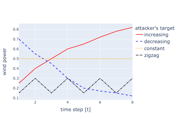
Among these, 3 targets correspond to various realistic scenarios. They aim to manipulate the model such that either increasing, decreasing, or constant wind power is predicted. In contrast, the fourth scenario corresponds to a zigzag line. This target was used to investigate how arbitrarily the forecasts can be manipulated. In addition, semi-targeted attacks were generated for a total of 4 different lower and upper bound constraints, as shown in Fig. 6.

Figure 6: Four different constraints considered for the semi-targeted PGD attacks: the forecast has to be between 0.75 and 1.0 (horizontal mesh), 0.5 and 0.75 (right diagonal), 0.25 and 0.5 (diagonal mesh), or between 0.0 and 0.25 (left diagonal)

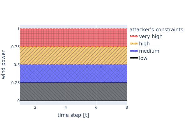
The objective of these constraints is to manipulate the model’s predictions so that the forecasted wind power is either in a low, medium, high, or very high range. Furthermore, we investigated to what extent the adversarial robustness of the two models can be increased with the help of adversarial training. For this purpose, adversarial examples were generated in each training iteration by perturbing every training sample using the untargeted PGD attack. The above described parameters were used here for the the untargeted PGD attack as well. The model was then trained on the adversarial examples only.
While the robustness of the two models to untargeted attacks was assessed using only the PRS, the robustness to semi-targeted and targeted attacks was quantified using all three scores (PRS, DRS, and TARS). They were calculated individually for each target and constraint of the attacker. This was done by first generating an adversarial example from every test sample. Then, the PRS, DRS and TARS were calculated sample-wise. Next, the average PRS, DRS, and TARS were calculated for each individual test dataset by averaging the scores of the respective test samples. Finally, the means and standard deviations of the average PRS, DRS and TARS were calculated from the 10 individual wind farm test datasets and the 8 Germany test datasets, respectively.

4 Results

4.1 Adversarial robustness of the LSTM model

The forecasting model for wind farms was quite robust to untargeted adversarial attacks with $\epsilon=0.15$, as Table 1 shows. While the ordinarily trained model achieved an average RMSE of 12.90% of installed capacity when not under attack, its performance deteriorated to an average RMSE of 15.30% when attacked by untargeted PGD attacks. The PRS was thus 0.79 in the case of untargeted PGD attacks. Noise attacks had an even lower impact on the prediction quality of the model and achieved an average PRS value of 0.96.
Semi-targeted PGD attacks had the highest impact when the constraint required the prediction of medium wind power, as shown in Table 2. For this constraint, an average TARS of 0.78 was obtained for the ordinarily trained model. For the other three constraints, the average TARS was 0.79 or more. Thus, the model was robust to semi-targeted PGD attacks as well.
As shown in Table 3, targeted PGD attacks with $\epsilon=0.15$ had a similar impact on the LSTM forecasting model for all four adversarial targets. Here, the ordinarily trained model achieved an average TARS value of 0.86 or greater for each of the attacker’s targets. It was thus very robust to this type of attack.

Table 1: Mean PRS and RMSE values with standard deviation for the LSTM forecasting model when attacked by noise attacks and untargeted PGD attacks

	ordinary training			adversarial training
attack	PRS	RMSE%		PRS	RMSE%
No attack	-	12.90 $\pm$ 1.21		-	13.24 $\pm$ 1.22
PGD	0.79 $\pm$ 0.02	15.30 $\pm$ 1.29		0.84 $\pm$ 0.02	14.99 $\pm$ 1.31
Noise	0.96 $\pm$ 0.01	13.01 $\pm$ 1.19		0.98 $\pm$ 0.00	13.29 $\pm$ 1.22

Table 2: Mean TARS, DRS, and PRS values with standard deviation for the LSTM forecasting model under semi-targeted PGD attacks

attacker’s	ordinary training			adversarial training
constraints	TARS	DRS	PRS	TARS	DRS	PRS
low	0.79 $\pm$ 0.02	0.81 $\pm$ 0.02	0.86 $\pm$ 0.02	0.84 $\pm$ 0.02	0.84 $\pm$ 0.02	0.90 $\pm$ 0.02
medium	0.78 $\pm$ 0.02	0.78 $\pm$ 0.02	0.86 $\pm$ 0.02	0.82 $\pm$ 0.02	0.82 $\pm$ 0.02	0.89 $\pm$ 0.02
high	0.80 $\pm$ 0.02	0.82 $\pm$ 0.03	0.86 $\pm$ 0.02	0.85 $\pm$ 0.03	0.85 $\pm$ 0.03	0.90 $\pm$ 0.02
very high	0.84 $\pm$ 0.02	0.87 $\pm$ 0.02	0.87 $\pm$ 0.02	0.88 $\pm$ 0.02	0.90 $\pm$ 0.02	0.91 $\pm$ 0.02

Table 3: Mean TARS, DRS, and PRS values with standard deviation for the LSTM forecasting model when attacked by targeted PGD attacks

attacker’s	ordinary training			adversarial training
target	TARS	DRS	PRS	TARS	DRS	PRS
increasing	0.89 $\pm$ 0.01	0.91 $\pm$ 0.01	0.88 $\pm$ 0.01	0.92 $\pm$ 0.01	0.94 $\pm$ 0.01	0.91 $\pm$ 0.02
decreasing	0.90 $\pm$ 0.01	0.91 $\pm$ 0.01	0.90 $\pm$ 0.01	0.93 $\pm$ 0.01	0.94 $\pm$ 0.01	0.93 $\pm$ 0.02
constant	0.86 $\pm$ 0.02	0.87 $\pm$ 0.02	0.88 $\pm$ 0.01	0.90 $\pm$ 0.02	0.90 $\pm$ 0.02	0.91 $\pm$ 0.02
zigzag	0.89 $\pm$ 0.01	0.89 $\pm$ 0.01	0.89 $\pm$ 0.01	0.92 $\pm$ 0.01	0.92 $\pm$ 0.01	0.93 $\pm$ 0.02

In order to achieve successful targeted PGD attacks on the ordinarily trained forecasting model, very strong perturbations of the wind speed time series were required, as the example in Figure 7 shows. Here, the attacked prediction did not closely match the attacker’s target until the perturbation magnitude was $\epsilon=3.0$. In addition, the perturbed wind speed time series often had a shape similar to the shape of the wind power forecast. This indicates that the model’s behavior was physically correct.

(a) While the original prediction (dotted) approximates the ground truth (dashed) very well, the attacked prediction (solid) converges to the attacker’s target (dash-dotted) with increasing maximum perturbation magnitude $\epsilon$

(b) As the perturbation magnitude $\epsilon$ rises, the perturbed wind speeds (solid) increasingly diverge from the original wind speeds (dotted). In addition, the shapes of the perturbed wind speeds often resemble the shapes of the attacked predictions in (a)

Figure 7: Four targeted PGD attacks with maximum perturbation magnitudes $\epsilon=0.15$ (left), $\epsilon=1.0$ (center-left), $\epsilon=2.0$ (center-right), and $\epsilon=3.0$ (right) on an exemplary prediction of the LSTM forecasting model. The figures show the impact of the attacks on (a) the wind power forecast and (b) the input data

With the help of adversarial training, the model’s robustness to PGD attacks and noise attacks could be slightly increased, as shown by the respective PRS values in Table 1 along with the TARS values in Table 2 and Table 3. However, when not under attack, the forecast accuracy of the model slightly deteriorated due to adversarial training. Thus, the average RMSE value between the model’s predictions and the ground truth on the test datasets was about 12.90% of installed capacity in the case of ordinary training, but 13.24% in the case of adversarial training.

4.2 Adversarial robustness of the CNN model

In contrast to the LSTM forecasting model for the wind farms, the CNN model for forecasting the wind power generation throughout Germany was very susceptible to PGD attacks with $\epsilon=0.15$. The average PRS value for untargeted PGD attacks on the ordinarily trained model was 0.05, as shown in Table 4. As a result of the untargeted PGD attacks, the average RMSE of the model deteriorated from 5.24% of installed capacity to 46.18%. Noise attacks resulted in an average PRS of 0.93 for the ordinarily trained model. Thus, they had a similarly small impact on the CNN forecasting model as on the LSTM forecasting model.
The ordinarily trained CNN model was also very vulnerable to semi-targeted and targeted PGD attacks. For the semi-targeted attacks, the TARS for all four constraints was 0.10 or less, as shown in Table 5. As Table 6 shows, the average TARS value for the targeted attacks with the increasing target was 0.01. For the zigzag shaped as well as the constant and decreasing target of the attacker, the average TARS was even 0.00.

Table 4: Mean PRS and RMSE values with standard deviation for the CNN forecasting model when attacked by noise attacks and untargeted PGD attacks

	ordinary training			adversarial training
attack	PRS	RMSE%		PRS	RMSE%
No attack	-	5.24 $\pm$ 1.17		-	6.22 $\pm$ 1.53
PGD	0.05 $\pm$ 0.04	46.18 $\pm$ 10.93		0.82 $\pm$ 0.08	7.77 $\pm$ 2.08
Noise	0.93 $\pm$ 0.04	5.22 $\pm$ 1.10		0.99 $\pm$ 0.00	6.21 $\pm$ 1.55

Table 5: Mean TARS, DRS, and PRS values with standard deviation for the CNN forecasting model under semi-targeted PGD attacks

attacker’s	ordinary training			adversarial training
constraints	TARS	DRS	PRS	TARS	DRS	PRS
low	0.10 $\pm$ 0.05	0.59 $\pm$ 0.15	0.12 $\pm$ 0.07	0.67 $\pm$ 0.11	0.71 $\pm$ 0.09	0.83 $\pm$ 0.07
medium	0.06 $\pm$ 0.04	0.18 $\pm$ 0.09	0.09 $\pm$ 0.06	0.46 $\pm$ 0.07	0.54 $\pm$ 0.07	0.64 $\pm$ 0.10
high	0.01 $\pm$ 0.02	0.04 $\pm$ 0.06	0.06 $\pm$ 0.06	0.61 $\pm$ 0.08	0.78 $\pm$ 0.07	0.62 $\pm$ 0.12
very high	0.01 $\pm$ 0.03	0.06 $\pm$ 0.09	0.03 $\pm$ 0.06	0.66 $\pm$ 0.09	0.89 $\pm$ 0.06	0.61 $\pm$ 0.11

Table 6: Mean TARS, DRS, and PRS values with standard deviation for the CNN forecasting model when attacked by targeted PGD attacks

attacker’s	ordinary training			adversarial training
target	TARS	DRS	PRS	TARS	DRS	PRS
increasing	0.01 $\pm$ 0.03	0.04 $\pm$ 0.07	0.07 $\pm$ 0.06	0.71 $\pm$ 0.08	0.90 $\pm$ 0.03	0.65 $\pm$ 0.11
decreasing	0.00 $\pm$ 0.01	0.01 $\pm$ 0.02	0.08 $\pm$ 0.05	0.77 $\pm$ 0.06	0.88 $\pm$ 0.03	0.73 $\pm$ 0.08
constant	0.00 $\pm$ 0.01	0.01 $\pm$ 0.02	0.15 $\pm$ 0.10	0.69 $\pm$ 0.08	0.85 $\pm$ 0.04	0.66 $\pm$ 0.12
zigzag	0.00 $\pm$ 0.00	0.00 $\pm$ 0.00	0.22 $\pm$ 0.08	0.79 $\pm$ 0.05	0.85 $\pm$ 0.05	0.79 $\pm$ 0.05

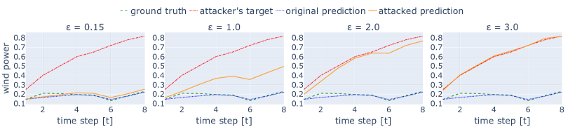
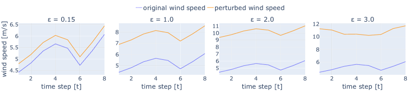
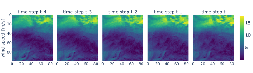
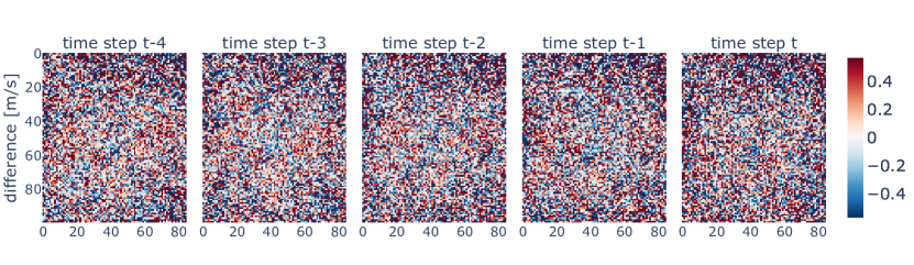
As an example, Figure 8 shows the impact of a PGD attack with the increasing adversarial target on an exemplary prediction. In this case, small perturbations of the weather maps had caused the model’s prediction to move close to the attacker’s target. As a result of the PGD attack, the wind speeds of the weather maps are both increased and decreased to varying degrees. Yet, the maximum perturbation magnitude is always less than 0.5 m/s. Although the differences between the perturbed weather maps and the original weather maps are visible, they are mostly inconspicuous.
The robustness of the CNN model to PGD attacks could be significantly increased with the help of adversarial training. For instance, the average PRS for the untargeted PGD attacks was 0.82 when adversarial training was used, see Table 4. For semi-targeted and targeted attacks, adversarial training resulted in the average TARS being above 0.46 for all the attacker’s constraints and above 0.69 for all the attacker’s targets, see Tables 5 and 6, respectively.
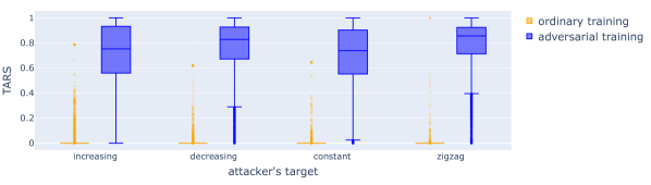
As shown in Figure 9, adversarial training had a positive effect on the robustness of the model not only on average, but indeed for most test samples. Thus, in the case of targeted PGD attacks, the 75th percentile of the TARS was below $4.49\cdot 10^{-7}$ for all four of the attacker’s targets when the model was trained ordinarily. When adversarial training was used instead, the 25th percentile of the TARS was above 0.55 for all four targets of the attacker. Although adversarial training significantly increased the robustness of the model, there still were individual samples for which the targeted PGD attacks were successful. In addition, adversarial training had a negative effect on the prediction accuracy of the model when not under attack. The average RMSE value between the model’s predictions and the ground truth was 5.24% of installed capacity on the test datasets for ordinary training, but 6.22% for adversarial training.

(a) While the original prediction (dotted) matches the ground truth (dashed) very well, the attacked prediction (solid) is much closer to the attacker’s target (dash-dotted) than to the ground truth

(b) The original wind speeds used to predict the last time step of the forecast ($t=8$)

(c) The wind speeds from (b) with the perturbations caused by the PGD attack

(d) Difference between the perturbed (c) and original (b) wind speeds, i.e., $x_{adv}-x$

Figure 8: A targeted PGD attack with perturbation magnitude $\epsilon=0.15$ on an exemplary prediction of the CNN forecasting model. The figures show (a) the impact of the attack on the wind power forecast as well as (b) the original input data, (c) the perturbed input data, and (d) the difference between the original and perturbed input data for the last time step of the forecast. All weather maps shown represent wind speeds across Germany in the unit m/s

Figure 9: TARS values of targeted PGD attacks on the CNN forecasting model for the increasing (left), decreasing (center-left), constant (center-right), and zigzag (right) target. The boxplots show that in the case of ordinary training (orange) the attacks are successful for most test samples. If adversarial training (blue) is used instead, the effects of the attacks are significantly reduced

5 Discussion

In this work, we investigated the adversarial robustness of two different wind power forecasting models. We developed the TARS to quantify the robustness of the models to targeted and semi-targeted adversarial attacks. Our results show that wind power forecasting models which make forecasts for individual wind farms are robust even to powerful adversarial attacks. It requires very strong perturbations of the input data to bias the model’s predictions toward the attacker’s target. However, these perturbations are such that they appear to fit the model’s predictions from a physical point of view. Thus, we hypothesize that the model behaves physically correct even in the case of attack.
On the other hand, wind power forecasting models, which use weather maps to produce forecasts for entire regions, are very vulnerable to adversarial attacks. Even small and barely perceptible perturbations of the input data are sufficient to falsify the forecasts almost arbitrarily. We suspect that this is due to the high dimensionality of the input data. Forecasting models for individual wind farms process very low-dimensional input data with only a few relevant features. In contrast, weather maps represent high-dimensional data with many features being relevant for large-scale wind power forecasting. This assumption is consistent with the study of [42], which showed that the generation of adversarial attacks benefits from higher dimensionality of input data in the classification setting. Note that the dimensionality of the input data we used is still comparatively low. In real applications, such as in [39], various other weather predictions are used besides wind speed forecasts, e.g., predictions for air pressure, air temperature, and air humidity. Such input data gives attackers even more attack possibilities.
We also studied adversarial training in order to protect the models from attacks. While adversarial training exorbitantly increased the robustness of the CNN forecasting model, it had only marginal effects on the robustness of the LSTM forecasting model. Adversarial training also slightly deteriorated the forecast accuracy of both models when not under attack. This finding is consistent with several studies in the classification setting [43, 44, 45], which state that there is a trade-off between robustness and accuracy. Therefore, an important direction for future work is to develop adversarial defenses that do not negatively impact the performance of forecasting models. An alternative approach could be to scale several robust wind power forecasts for individual wind farms up to a region, as outlined in [46]. However, it remains to be examined whether such an upscaling approach for regional forecasts is as accurate as forecasts generated from weather maps. Another important direction for future work is to extend our method used to generate targeted attacks on forecasting models. Currently, we select the various adversarial targets very carefully by hand. However, it would be desirable to have techniques for automatically generating realistic, application-specific adversarial targets. Such techniques would allow a more comprehensive robustness evaluation.

6 Conclusion

In this study, we have shown that the use of Deep Learning (DL) for wind power forecasting can pose a security risk. In general, our results are relevant for forecasting in power systems, including solar power and load flow forecasting, among others. Adversarial attacks also pose a threat to forecasting models used in other critical infrastructures, for example, the financial and insurance sectors. DL-based forecasting models which obtain input data from safety-critical interfaces should therefore always be tested for their vulnerability to adversarial attacks before being deployed. In order to appropriately quantify the robustness of such models, we proposed the Total Adversarial Robustness Score (TARS). In case of high vulnerability, adequate defense mechanisms, such as adversarial training, should be used to protect the models from attacks. Finally, our work represents a first study of targeted adversarial attacks for DL-based regression models, and we expect this to be a promising area for future research.

Code availability

The code for the experiments in this paper, as well as the associated visualizations, is available at https://github.com/FraunhoferIEE/taaowpf.

Appendix A Adversarial robustness scores

The following figures are intended to illustrate the behavior of the three evaluation metrics TARS, DRS, and PRS. While Figure 10 shows the evolution of the PRS, Figure 11 demonstrates the behavior of the DRS, and Figure 12 depicts the trajectory of the TARS.

Figure 10: Evolution of the PRS for increasing values of $\operatorname{RMSE}\left(\hat{y}_{adv},y\right)$, where $\operatorname{RMSE}\left(\hat{y},y\right)=2$ (solid), $3$ (dashed) and $4$ (dotted). When $\operatorname{RMSE}\left(\hat{y}_{adv},y\right)$ tends to infinity, the PRS converges to zero

Figure 11: Evolution of the DRS for decreasing values of $\operatorname{RMSE}\left(\hat{y}_{adv},y_{adv}\right)$, where $\operatorname{RMSE}\left(\hat{y},y_{adv}\right)=2$ (solid), $3$ (dashed) and $4$ (dotted). When $\operatorname{RMSE}\left(\hat{y}_{adv},y_{adv}\right)$ tends to zero, the DRS converges to zero as well

Figure 12: Trajectory of the $\operatorname{TARS}_{\beta}$ with $\beta=1$ for different values of PRS and DRS. If either the PRS or the DRS take values close to zero, the value of the TARS is also close to zero. Conversely, the value of the TARS is close to one only if both the PRS and the DRS take values close to one

Appendix B Data

In the following, the two datasets used for the experiments in this work are described in more detail.

B.1 Dataset on wind power generation from wind farms

For the prediction of the power generation of individual wind farms, we used the publicly available GEFCom2014 wind forecasting dataset [36]. This dataset consists of normalized wind power measurements from 10 wind farms in Australia. All wind power measurements were normalized to the nominal capacity of the respective wind farm and therefore took values between 0 and 1. In addition, the dataset contains predictions of the zonal wind speed $u$ (wind parallel to latitude) and the meridional wind speed $v$ (wind parallel to longitude) at 100m above ground for the location of each wind farm. For simplicity, we calculated the horizontal wind speed $V_{h}$ at 100m above the ground from the zonal and meridional wind speeds for our experiments:

$$V_{h}=\sqrt{u^{2}+v^{2}}$$ (14)

Thus, the wind power and wind speed data for the wind farms are each a univariate time series. The wind speed data of the wind farms were standardized separately with the z-score. Hence, the standardized wind speed of each wind farm had a mean of 0 and a standard deviation of 1. The data is available for the years 2012 and 2013 with a temporal resolution of 1 hour. For the training and hyperparameter tuning of the LSTM forecasting models, the data for each wind farm was split into a training, validation, and test dataset. The resulting 10 training datasets each contained data from January 2012 to June 2013, with the last week of each quarter used for the corresponding validation dataset. Thus, the training data for each wind farm spanned a total of 16.5 months, while the validation data covered 6 weeks. The test datasets consisted of data from July 2013 to December 2013. The individual data samples were then constructed using a one-step sliding window that moved across the hourly values.

B.2 Dataset on wind power generation in Germany

The wind power generated throughout Germany was predicted using wind speed forecasts in the form of weather maps. The forecasts for horizontal wind speed at about 100m above the ground were calculated based on the zonal and meridional wind speed forecasts from the ICON-EU model of the German Meteorological Service (DWD). The wind speed forecasts had an hourly temporal resolution. They were aggregated to a 100 × 85 grid with a spatial resolution of 10km x 10km using bilinear interpolation. The grid covered all of Germany, and the center of the top left grid cell had the latitude 55.866 and longitude 3.071. The historical wind power data we used as target values is real and publicly available, as are the wind speed forecasts. Historical data on onshore wind energy generated across Germany were obtained from the website of the European Network of Transmission System Operators (ENTSO-E) . The wind power measurements were normalized by the installed wind power capacity in Germany and therefore only took values between 0 and 1. The dataset covered the period from January 2019 to June 2021. It was divided into 8 different subsets using blocked cross-validation. Each subset was further subdivided into a training, validation, and test dataset. These were chosen so that there was only a 50% overlap between successive training datasets and no overlap between test datasets. The time periods of the training and test datasets of the 8 cross-validation subsets are shown in Table 7.

Table 7: The training and test periods of the 8 cross-validation subsets of the dataset used for wind power forecasting across Germany

Cross-validation subset	Training	Test
1	January 2019 - June 2019	July 2019 - September 2019
2	April 2019 - September 2019	October 2019 - December 2019
3	July 2019 - December 2019	January 2020 - March 2020
4	October 2019 - March 2020	April 2020 - June 2020
5	January 2020 - June 2020	July 2020 - September 2020
6	April 2020 - September 2020	October 2020 - December 2020
7	July 2020 - December 2020	January 2021 - March 2021
8	October 2020 - March 2021	April 2021 - June 2021

The last four days of each month of a training dataset were used as the corresponding validation dataset. Thus, each training dataset spanned a total of about 5.2 months, while the validation datasets covered 24 days each. The eight test datasets contained 3 months each. The wind speed predictions of each subset were standardized separately using the z-score. Thus, the standardized wind speed predictions of each subset had a mean of 0 and a standard deviation of 1. The individual data samples were then constructed using a one-step sliding window.

Appendix C Forecasting models

In the following, the two wind power forecasting models, whose adversarial robustness was investigated in this work, are described in more detail.

C.1 LSTM forecasting model

Similar to [38], we used an encoder-decoder LSTM [37] for a multistep-ahead prediction of the power generated by individual wind farms. This model consisted of an encoder LSTM network and a decoder LSTM network. First, the encoder network encoded an input sequence consisting of the wind power measurements for the past 12 hours into a latent representation. This latent representation was then used to initialize the hidden state and cell state of the decoder network. The decoder then sequentially generated a wind power forecast for the next 8 hours with a time resolution of one hour. Here, the decoder used the wind speed forecast of time $t$ along with the predicted wind power of the previous time $t-1$ to predict the wind power for time $t$, where $t=1,...,8$. In the case where $t=1$, the decoder used the real wind power measurement from the current time $t=0$ instead of a prediction.
The training and validation datasets of the wind farm in zone 1 of the GEFCom2014 dataset were used to tune the hyperparameters. The following hyperparameters of the model were optimized using the HyperBand method [47]: number of layers, hidden size, learning rate, and length of the input sequence of wind power measurements for the encoder. We used the asynchronous HyperBand algorithm from Ray Tune [48] with 1000 trials and the default parameter settings. Only the grace period was set to 20 to avoid stopping trials too early. After tuning the hyperparameters, the encoder network consisted of one LSTM layer with 32 neurons. The decoder network also consisted of one LSTM layer with 32 neurons, but followed by a dense layer with one neuron and a Leaky ReLU activation function. The loss function used was the MSE loss. As optimizer, Adam [49] was used. The initial learning rate was 0.01 and was reduced by a factor of 0.1 each time the validation loss did not improve over 10 epochs, using a learning rate scheduler. For this purpose, PyTorch’s [50] ReduceLROnPlateau learning rate scheduler was used with the default parameter settings. The maximum number of epochs was constrained to 100. Preliminary experiments have shown that this number is sufficient for convergence of the model’s training. In addition, early stopping was used to stop the training as soon as the validation loss did not improve within 15 epochs. Here, the EarlyStopping callback from PyTorch Lightning [51] was used with the default parameter settings. Only the patience parameter was chosen as 15 epochs, since this improved the model’s performance in preliminary experiments.

C.2 CNN forecasting model

A new approach for forecasting the generated wind power in large-scale regions was proposed by [39]. In this approach, the problem of wind power forecasting is divided into two distinct subproblems, each of which is solved separately. The first step consists of generating very accurate weather forecasts using a suitable weather prediction model. The second step then consists of generating the wind power forecast using the weather forecasts. For this purpose, a separate power estimation model is applied to estimate the wind power for a future point in time using the predicted weather maps for that point in time and previous points in time.
We used this approach in order to make an 8h forecast with one-hour resolution for the wind energy generated throughout Germany. To make a forecast for time $t$, the model received a stack of 5 weather maps as input. These consisted of the forecasts for the horizontal wind speed at 100m above ground level for the 5 hours leading up to the estimation time, i.e., points in time $t-4,...,t$. Here, the wind speed prediction of each point in time represented a separate channel. Thus, the dimension of the input data for a prediction for time $t$ was 5 × 100 × 85 (channels × pixel height × pixel width). For estimating the wind power based on the 5 weather maps, we used a ResNet-34 [40], followed by a dense layer with one neuron and a Leaky ReLU activation function in the output layer. This model was then sequentially applied to the input data and estimated the generated wind power step-by-step for points in time $t=1,...,8$. For training the model, MSE loss was used. As optimizer we used Adam. The maximum number of epochs was limited to 100. Preliminary experiments have shown that this number is sufficient for convergence of the model’s training. The initial learning rate was 0.001, which is the default value of PyTorch’s [50] Adam optimizer. It was reduced by a factor of 0.1 each time the validation loss did not improve within 10 epochs. For the CNN model, we used early stopping and the ReduceLROnPlateau learning rate scheduler in the same way as for the LSTM model, see Section C.1 for a detailed description.

References

- [1] Huaizhi Wang, Zhenxing Lei, Xian Zhang, Bin Zhou, and Jianchun Peng. A review of deep learning for renewable energy forecasting. Energy Conversion and Management, 198:111799, 2019.
- [2] Ghadah Alkhayat and Rashid Mehmood. A review and taxonomy of wind and solar energy forecasting methods based on deep learning. Energy and AI, 4:100060, 2021.
- [3] Umweltbundesamt. Renewable Energies in Germany: Data on the Development in 2021. Renewable energies in Germany. German Environment Agency, 2022.
- [4] Sheraz Aslam, Herodotos Herodotou, Syed Muhammad Mohsin, Nadeem Javaid, Nouman Ashraf, and Shahzad Aslam. A survey on deep learning methods for power load and renewable energy forecasting in smart microgrids. Renewable and Sustainable Energy Reviews, 144:110992, 2021.
- [5] Christian Szegedy, Wojciech Zaremba, Ilya Sutskever, Joan Bruna, Dumitru Erhan, Ian Goodfellow, and Rob Fergus. Intriguing properties of neural networks. arXiv preprint arXiv:1312.6199, 2013.
- [6] Ian J Goodfellow, Jonathon Shlens, and Christian Szegedy. Explaining and harnessing adversarial examples. arXiv preprint arXiv:1412.6572, 2014.
- [7] Carla Goncalves, Pierre Pinson, and Ricardo J Bessa. Towards data markets in renewable energy forecasting. IEEE Transactions on Sustainable Energy, 12(1):533–542, 2020.
- [8] Hassan Ismail Fawaz, Germain Forestier, Jonathan Weber, Lhassane Idoumghar, and Pierre-Alain Muller. Adversarial attacks on deep neural networks for time series classification. In 2019 International Joint Conference on Neural Networks (IJCNN), pages 1–8. IEEE, 2019.
- [9] Mubarak G Abdu-Aguye, Walid Gomaa, Yasushi Makihara, and Yasushi Yagi. Detecting adversarial attacks in time-series data. In ICASSP 2020-2020 IEEE International Conference on Acoustics, Speech and Signal Processing (ICASSP), pages 3092–3096. IEEE, 2020.
- [10] Pradeep Rathore, Arghya Basak, Sri Harsha Nistala, and Venkataramana Runkana. Untargeted, targeted and universal adversarial attacks and defenses on time series. In 2020 International Joint Conference on Neural Networks (IJCNN), pages 1–8. IEEE, 2020.
- [11] Alexey Kurakin, Ian J Goodfellow, and Samy Bengio. Adversarial examples in the physical world. In Artificial intelligence safety and security, pages 99–112. Chapman and Hall/CRC, 2018.
- [12] Fazle Karim, Somshubra Majumdar, and Houshang Darabi. Adversarial attacks on time series. IEEE transactions on pattern analysis and machine intelligence, 43(10):3309–3320, 2020.
- [13] Samuel Harford, Fazle Karim, and Houshang Darabi. Adversarial attacks on multivariate time series. arXiv preprint arXiv:2004.00410, 2020.
- [14] Scott Alfeld, Xiaojin Zhu, and Paul Barford. Data poisoning attacks against autoregressive models. In Proceedings of the AAAI Conference on Artificial Intelligence, volume 30, 2016.
- [15] Andre T Nguyen and Edward Raff. Adversarial attacks, regression, and numerical stability regularization. arXiv preprint arXiv:1812.02885, 2018.
- [16] Lucas Richter, Malte Lehna, Sophie Marchand, Christoph Scholz, Alexander Dreher, Stefan Klaiber, and Steve Lenk. Artificial intelligence for electricity supply chain automation. Renewable and Sustainable Energy Reviews, 163:112459, 2022.
- [17] Lei Cui, Youyang Qu, Longxiang Gao, Gang Xie, and Shui Yu. Detecting false data attacks using machine learning techniques in smart grid: A survey. Journal of Network and Computer Applications, 170:102808, 2020.
- [18] Saeed Ahmadian, Heidar Malki, and Zhu Han. Cyber attacks on smart energy grids using generative adverserial networks. In 2018 IEEE Global Conference on Signal and Information Processing (GlobalSIP), pages 942–946. IEEE, 2018.
- [19] Ali Sayghe, Junbo Zhao, and Charalambos Konstantinou. Evasion attacks with adversarial deep learning against power system state estimation. In 2020 IEEE Power & Energy Society General Meeting (PESGM), pages 1–5. IEEE, 2020.
- [20] Fiammetta Marulli and Corrado Aaron Visaggio. Adversarial deep learning for energy management in buildings. In SummerSim, pages 50–1, 2019.
- [21] Iman Niazazari and Hanif Livani. Attack on grid event cause analysis: An adversarial machine learning approach. In 2020 IEEE Power & Energy Society Innovative Smart Grid Technologies Conference (ISGT), pages 1–5. IEEE, 2020.
- [22] Xingyu Zhou, Yi Li, Carlos A Barreto, Jiani Li, Peter Volgyesi, Himanshu Neema, and Xenofon Koutsoukos. Evaluating resilience of grid load predictions under stealthy adversarial attacks. In 2019 Resilience Week (RWS), volume 1, pages 206–212. IEEE, 2019.
- [23] Yize Chen, Yushi Tan, and Baosen Zhang. Exploiting vulnerabilities of load forecasting through adversarial attacks. In Proceedings of the Tenth ACM International Conference on Future Energy Systems, pages 1–11, 2019.
- [24] Ningkai Tang, Shiwen Mao, and R Mark Nelms. Adversarial attacks to solar power forecast. In 2021 IEEE Global Communications Conference (GLOBECOM), pages 1–6. IEEE, 2021.
- [25] Zhou Wu, Gan Luo, Zhile Yang, Yuanjun Guo, Kang Li, and Yusheng Xue. A comprehensive review on deep learning approaches in wind forecasting applications. CAAI Transactions on Intelligence Technology, 7(2):129–143, 2022.
- [26] Yao Zhang, Fan Lin, and Ke Wang. Robustness of short-term wind power forecasting against false data injection attacks. Energies, 13(15):3780, 2020.
- [27] Han Xu, Yao Ma, Hao-Chen Liu, Debayan Deb, Hui Liu, Ji-Liang Tang, and Anil K Jain. Adversarial attacks and defenses in images, graphs and text: A review. International Journal of Automation and Computing, 17(2):151–178, 2020.
- [28] Jonas Rauber, Wieland Brendel, and Matthias Bethge. Foolbox: A python toolbox to benchmark the robustness of machine learning models. arXiv preprint arXiv:1707.04131, 2017.
- [29] Jonas Rauber and Matthias Bethge. Fast differentiable clipping-aware normalization and rescaling. arXiv preprint arXiv:2007.07677, 2020.
- [30] Nicholas Carlini, Anish Athalye, Nicolas Papernot, Wieland Brendel, Jonas Rauber, Dimitris Tsipras, Ian Goodfellow, Aleksander Madry, and Alexey Kurakin. On evaluating adversarial robustness. arXiv preprint arXiv:1902.06705, 2019.
- [31] Aleksander Madry, Aleksandar Makelov, Ludwig Schmidt, Dimitris Tsipras, and Adrian Vladu. Towards deep learning models resistant to adversarial attacks. arXiv preprint arXiv:1706.06083, 2017.
- [32] Shilin Qiu, Qihe Liu, Shijie Zhou, and Chunjiang Wu. Review of artificial intelligence adversarial attack and defense technologies. Applied Sciences, 9(5):909, 2019.
- [33] Naveed Akhtar, Ajmal Mian, Navid Kardan, and Mubarak Shah. Advances in adversarial attacks and defenses in computer vision: A survey. IEEE Access, 9:155161–155196, 2021.
- [34] Jan Hendrik Metzen, Tim Genewein, Volker Fischer, and Bastian Bischoff. On detecting adversarial perturbations. arXiv preprint arXiv:1702.04267, 2017.
- [35] Ron Bitton, Nadav Maman, Inderjeet Singh, Satoru Momiyama, Yuval Elovici, and Asaf Shabtai. Evaluating the cybersecurity risk of real-world, machine learning production systems. ACM Computing Surveys, 55(9):1–36, 2023.
- [36] Tao Hong, Pierre Pinson, Shu Fan, Hamidreza Zareipour, Alberto Troccoli, and Rob J Hyndman. Probabilistic energy forecasting: Global energy forecasting competition 2014 and beyond, 2016.
- [37] Ilya Sutskever, Oriol Vinyals, and Quoc V Le. Sequence to sequence learning with neural networks. Advances in neural information processing systems, 27, 2014.
- [38] Kuan Lu, Wen Xue Sun, Xin Wang, Xiang Rong Meng, Yong Zhai, Hong Hai Li, and Rong Gui Zhang. Short-term wind power prediction model based on encoder-decoder lstm. In IOP Conference Series: Earth and Environmental Science, volume 186, page 012020. IOP Publishing, 2018.
- [39] Sebastian BM Bosma and Negar Nazari. Estimating solar and wind power production using computer vision deep learning techniques on weather maps. Energy Technology, 10(8):2200289, 2022.
- [40] Kaiming He, Xiangyu Zhang, Shaoqing Ren, and Jian Sun. Deep residual learning for image recognition. In Proceedings of the IEEE conference on computer vision and pattern recognition, pages 770–778, 2016.
- [41] Jan Frederick Unnewehr, Eddy Jalbout, Christopher Jung, Dirk Schindler, and Anke Weidlich. Getting more with less? why repowering onshore wind farms does not always lead to more wind power generation–a german case study. Renewable Energy, 180:245–257, 2021.
- [42] Nandish Chattopadhyay, Anupam Chattopadhyay, Sourav Sen Gupta, and Michael Kasper. Curse of dimensionality in adversarial examples. In 2019 International Joint Conference on Neural Networks (IJCNN), pages 1–8. IEEE, 2019.
- [43] Dimitris Tsipras, Shibani Santurkar, Logan Engstrom, Alexander Turner, and Aleksander Madry. Robustness may be at odds with accuracy. arXiv preprint arXiv:1805.12152, 2018.
- [44] Aditi Raghunathan, Sang Michael Xie, Fanny Yang, John C Duchi, and Percy Liang. Adversarial training can hurt generalization. arXiv preprint arXiv:1906.06032, 2019.
- [45] Hongyang Zhang, Yaodong Yu, Jiantao Jiao, Eric Xing, Laurent El Ghaoui, and Michael Jordan. Theoretically principled trade-off between robustness and accuracy. In International conference on machine learning, pages 7472–7482. PMLR, 2019.
- [46] Jaesung Jung and Robert P Broadwater. Current status and future advances for wind speed and power forecasting. Renewable and Sustainable Energy Reviews, 31:762–777, 2014.
- [47] Lisha Li, Kevin Jamieson, Giulia DeSalvo, Afshin Rostamizadeh, and Ameet Talwalkar. Hyperband: A novel bandit-based approach to hyperparameter optimization. The Journal of Machine Learning Research, 18(1):6765–6816, 2017.
- [48] Richard Liaw, Eric Liang, Robert Nishihara, Philipp Moritz, Joseph E Gonzalez, and Ion Stoica. Tune: A research platform for distributed model selection and training. arXiv preprint arXiv:1807.05118, 2018.
- [49] Diederik P Kingma and Jimmy Ba. Adam: A method for stochastic optimization. arXiv preprint arXiv:1412.6980, 2014.
- [50] Adam Paszke, Sam Gross, Francisco Massa, Adam Lerer, James Bradbury, Gregory Chanan, Trevor Killeen, Zeming Lin, Natalia Gimelshein, Luca Antiga, et al. Pytorch: An imperative style, high-performance deep learning library. Advances in neural information processing systems, 32, 2019.
- [51] William Falcon et al. Pytorch lightning. GitHub. Note: https://github. com/PyTorchLightning/pytorch-lightning, 3(6), 2019.