Implicit Visual Bias Mitigation by Posterior Estimate Sharpening of a Bayesian Neural Network

Abstract

The fairness of a deep neural network is strongly affected by dataset bias and spurious correlations, both of which are usually present in modern feature-rich and complex visual datasets. Due to the difficulty and variability of the task, no single de-biasing method has been universally successful. In particular, implicit methods not requiring explicit knowledge of bias variables are especially relevant for real-world applications. We propose a novel implicit mitigation method using a Bayesian neural network, allowing us to leverage the relationship between epistemic uncertainties and the presence of bias or spurious correlations in a sample. Our proposed posterior estimate sharpening procedure encourages the network to focus on core features that do not contribute to high uncertainties. Experimental results on three benchmark datasets demonstrate that Bayesian networks with sharpened posterior estimates perform comparably to prior existing methods and show potential worthy of further exploration.

1 Introduction

In a perfectly unbiased world, every possible combination of features would be equally present in every sample set. Unfortunately, it has become increasingly apparent that societal and historical biases are prevalent in every domain. Furthermore, even if it were always feasible to obtain a balanced dataset, this in itself does not ensure a fair model, as relative quantities are not the sole contributor towards bias [41, 26]. Not only are biased datasets pervasive, but algorithms themselves can even amplify bias [50, 18].

Particularly in the visual domain, it is not realistic to assume a comprehensive knowledge of all bias variables in a dataset, let alone know where they occur across the training data. In high-impact domains highly susceptible to dataset bias, including medicine, finance, welfare, and crime, confidentiality and privacy requirements prohibit general use of metadata which might specify presence of bias variables in training sets. Furthermore, in most cases population bias makes balanced sampling impossible. The implications and consequences [11, 9, 28, 8]  of unfair models built using such biased datasets are disheartening and intolerable.

Recently, various studies propose implicit mitigation methods for neural networks [42, 27, 46, 4]. Yet many challenges still remain. Sample imbalances between minority and majority groups can be too steep to overcome without overfitting [43, 4, 36], learning spurious correlations is often much easier than learning the desired core features [18], and some bias-conflicting samples are simply more difficult to learn than others [41]. Additionally, studies comparing results for multiple methods on more than one visual bias benchmark dataset indicate that no single mitigation method is universally effective [34, 42, 18].

We contribute towards a better understanding and exploration of visual bias mitigation by proposing a novel implicit mitigation method which leverages the correlation between uncertainties and bias-conflicting samples. Epistemic uncertainties in the Bayesian paradigm arise from lack of knowledge – missing information or data – and decrease given a more comprehensive distribution of data. This contrasts with aleatoric uncertainty, or data “noise" uncertainty which is irreducible since probabilistic variations are present irrespective of the dataset size. Thus, a more balanced distribution of data (in both quantity and ease of learning) will reduce epistemic uncertainties. We can directly leverage this for implicit bias mitigation.

A few recent works have also used this correlation. Branchaud-Charron et al. [7] show Bayesian Active Learning by Disagreement (BALD) [15] can help mitigate bias against relying on spurious correlations through re-balancing the dataset via an acquisition scheme which greedily reduces epistemic uncertainty. Khan et al. [22] use Bayesian uncertainty estimates to deal with class imbalance by weighting the loss function to move learned class boundaries away from more uncertain classes. This focuses primarily on class-level bias in the class imbalance scenario, with some consideration for sample-level bias; our proposed method focuses solely on sample-level bias as we do not expect bias to be constrained to classes. Epistemic uncertainties are also used in a previous study [36] (EpiWt) to dynamically weight samples during training, but this approach suffers from the same overfitting problem as both explicit and implicit up-weighting methods.

Contributing to this body of literature, we propose a novel posterior estimate sharpening approach, which focuses on uncertainty-guided implicit feature re-weighting in the classification layers of a Bayesian neural network. In addition to showing potential compared against other methods, our sharpening approach also provides post-inference uncertainty estimates which can be useful for a variety of purposes.

2 Related Work

Prior mitigation methods can be categorized as explicit or implicit. Explicit approaches require knowing the bias variables and which training samples are bias-aligned. Various works have experimented with re-weighting or re-sampling, the intuitive approach by which the minority samples are made to appear more often, thus encouraging the model not to leverage undesired correlations. This can be done via sampling probability [10, 21], loss weighting [12], or synthetically generating or augmenting data to balance out or encourage learning of certain features [19, 16].

Other methods focus on discouraging the representation portion of the network from encoding the biases. This can be accomplished through adversarial learning [48, 40], or by manipulating the feature representations in latent space to disentangle the spurious and core features [38, 37].

Another category of works explicitly learn the bias variable, in order to then unlearn it or adjust the model decisions based on this knowledge [14, 42]. Alvi et al. [3] propose a variant of this through “fairness through blindness", simultaneously learning the target task while learning to ignore the bias variables. However, these methods are vulnerable to redundant encoding [26], or learning combinations of other perhaps unlabeled bias variables as a proxy for the chosen bias variables.

The knowledge of bias variables can also be used to group the training data into subgroups for training fairer models. Group distributionally robust optimization (gDRO) suggests sub-grouping data according to their bias and class variables, and optimizes such that the model generalizes best over all groups [30]. Predictive group invariance (PGI) [1] also groups data according to bias variables and encourages matched predictive distributions across the groups, penalizing learning spurious features that do not appear across all groups. Both [30, 1] assume bias variables are specified in the training set, but also propose ways to infer groupings implicitly from the data. Similarly, but with a reinforcement learning setup, [41] propose an adaptive margin loss function which computes ideal margins between groups.

In contrast, implicit methods do not assume any prior knowledge of bias variables in the data. One such category of implicit methods leverages the observation that networks themselves can sometimes identify when they have learned spurious features as they are more easily learned, but, relying on them still results in misclassifications for a minority. Learning from Failure (LfF) [27], Learning with Biased Committee (LWBC) [23], and approaches by Bahng et al. [5] and Sanh et al. [31] exploit the failures of one or more normal or bias-amplifying networks to inform a de-biased network. These methods attempt to minimise the effect of bias-aligned training samples, some by actually removing samples from the training set shown to the target network.

Other methods explore implicit versions of up-weighting or re-sampling, by discovering sparse areas of the feature space [4] or dynamically identifying samples more likely to be bias-conflicting [36]. Du et al. [13] de-bias the classification head of the network by training on neutralized representations of training data. This requires knowing when bias variables appear in the training samples (or at least being able to predict using some other model) in order to adjust the representations.

Another category of implicit methods change the loss function to reward learning a fairer model; Xu et al. [46] implement this via a false positive rate penalty loss, and Pezeshki et al. [29] through Spectral Decoupling (SD), an adjusted L2 loss encouraging feature decoupling and discouraging learning features at the expense of learning another. SD allows the learning of simple correlations but not unilaterally, resulting in the preservation of minority core features.

Recently, Shrestha et al. [35] open a promising new direction of work, leveraging architectural inductive biases with an adaptable architecture (OccamNets) which allows the network to favor simpler solutions when needed. The resulting model prefers focusing on smaller visual regions for predictions yet does not constrain all samples to rely on the same complexity of hypotheses, as optimal “exit" locations in the architecture are learned per sample.

Our proposed implicit method shares intuition and motivation with many of these approaches, as we discuss further in Section 3.4.

3 Methodology

3.1 Premise

For a Bayesian neural network with parameters $\boldsymbol{\theta}$, posterior $p(\boldsymbol{\theta}~{}\mid D,\boldsymbol{x})$, class-labelled training data $D=(X,Y)$, and test sample $\boldsymbol{x}_{i}$, the predictive posterior distribution for a given target class $\boldsymbol{y}_{i}$ is as follows:

$$p(\boldsymbol{y}_{i}\mid D,\boldsymbol{x}_{i})=\int p(\boldsymbol{y}_{i}\mid\boldsymbol{\theta},\boldsymbol{x}_{i})p(\boldsymbol{\theta}\mid D)d\boldsymbol{\theta}$$ (1)

While this itself is intractable, stochastic gradient MCMC (SG-MCMC [44]) is a tractable variation of the gold standard Markov chain Monte Carlo (MCMC) algorithm, and uses the stochastic gradient over mini-batches with an additional Gaussian noise bound instead of the gradient over the whole training distribution. Furthermore, for faster convergence and a more thorough exploration of the multimodal distributions prevalent in deep neural networks, we adopt the cyclical learning rate schedule introduced in [49] known as cyclical SG-MCMC, or cSG-MCMC. Larger learning step phases provide a warm restart to the subsequent smaller steps constituting the sampling phase.

The final estimated posterior of the Bayesian network consists of $\boldsymbol{\Theta}=\{\boldsymbol{\theta_{1}},...\boldsymbol{\theta_{M}}\}$, $M$ moments sampled from the posterior over all trainable parameters, taken during the sampling phases of each learning cycle. With functional model $\boldsymbol{\Phi}$ representing the neural network, the approximate predictive mean $\boldsymbol{\mu}_{i}$ and output class prediction $\boldsymbol{\hat{y}}_{i}$ for sample $\boldsymbol{x}_{i}$ are:

$$\boldsymbol{\mu}_{i}\approx\frac{1}{M}\sum_{m=1}^{M}\boldsymbol{\Phi}_{\theta_{m}}(\boldsymbol{x}_{i})$$ (2)

$$\boldsymbol{\hat{y}}_{i}=\textup{argmax}\left(\boldsymbol{\mu}_{i}\right)$$ (3)

The epistemic uncertainty corresponding to this prediction is:

$$\boldsymbol{\sigma}_{i}\approx\frac{1}{M}\sqrt{\sum_{m=1}^{M}\left(\boldsymbol{\Phi}_{\boldsymbol{\theta}_{m}}(\boldsymbol{x}_{i})-\boldsymbol{\mu}_{i}\right)^{2}}$$ (4)

which for any given sample is an indicator of model confidence in its prediction based on the information given. We refer readers to [20] for a more in-depth presentation of Bayesian neural networks and their implementation.

3.2 Bias and Uncertainties

Bias-conflicting samples tend to have higher epistemic uncertainties than their bias-aligned counterparts [17, 2, 36]. These epistemic uncertainties arise from the classification, not representation, portions of the network despite the learned representations being arguably “biased representations" [13]. We can briefly explore these two claims on a toy synthetic dataset which we call Biased Synbols. We choose Synbols [25] as the tool to build Biased Synbols as we can easily control the resolution and features in each generated image. The foreground of each $224$ x $224$ image is a character displayed in a font chosen randomly from a large selection of fonts, and the texture of the character is a random natural scene, cropped to fit the character mask. The background behind the character is a 2-color gradient. We introduce four types of bias as shown in Figure 1.

Figure 1: One sample from class “s" of our toy dataset Biased-Synbols with controllable bias variables (left to right): texture of letter, spurious square placed in random corner, resolution of whole image, and gray-scale.

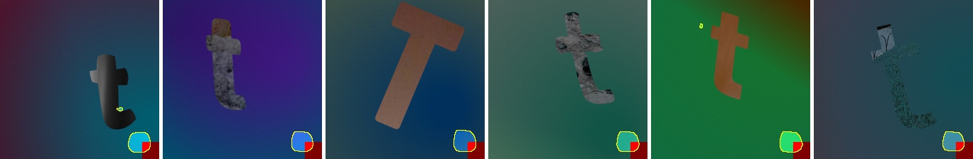
Figure 2: The six training images for which kernel 0, convolutional layer 4 (top) and kernel 10, convolution layer 2 (bottom) from AlexNet most strongly activate. The first kernel has identified a core feature for class “s", whereas the second corresponds to the spurious or bias feature rather than the character.

We generate a two letter (“s" and “t") binary classification task with train/val/test splits of 20k/5k/5k and train Bayesian AlexNet on four versions of Biased Synbols, each with a different bias variable and $p_{bias}=0.95$ for the “s" class and $p_{bias}=0.05$ for the “t". In each case, the bias-conflicting samples have higher mean group uncertainties than the bias-aligned (a mean increase by 0.15, 0.16, 0.09, and 0.20 for the four variables shown in Figure 1 respectively, for normalized uncertainties between 0.0-1.0).

Next, we identify where the discrepancies in uncertainties arise from in the network. We find indiscernible difference in uncertainties by averaging the uncertainties across the features extracted directly after the final convolutional layer. To further confirm, we perform network dissection [6]. on Biased Synbols with the spurious square in a random corner. Network dissection measures the alignment between convolutional kernel activations and any concept, which can be defined by segmentation masks on the dataset. As the square bias variable is generally spatially distinct from the core feature, i.e. the character shape, we can dissect the network to locate which convolutional kernels are most strongly activated by the former (Figure 2). For every convolutional layer in AlexNet, we compute the intersection-over-union (IoU) of the square with the thresholded kernel activation heatmaps, and measure correlation between these IoUs and the kernel uncertainties. The Pearson correlations per layer are -0.01, -0.03, 0.13, -0.07, and 0.17, strongly indicating no clear correlation; thus, simply learning features associated with bias variables does not create discrepancies in uncertainties.

These observations motivate our focus on the classification head and the uncertainties induced by learning a biased feature weighting in the classification layers of the network.

3.3 Posterior Estimate Sharpening

We propose a sharpening procedure (Algorithm 1) which further fine-tunes the classification layers of each Monte-Carlo sample from the Bayesian posterior using a multi-component loss function. We freeze the representation portion of the network during this procedure because (1) we aim to learn re-weighting of learned features in the classification head only, (2) updating the representation network can change the feature representations, thus complicating the re-weighting goal, and (3) experimental evidence backs these intuitions, showing a drastic drop in both performance and model fairness when the whole network is fine-tuned. Thus, when we refer to posterior estimates for sharpening, we are referring to $\boldsymbol{\theta}_{c}$, where each posterior sample $\boldsymbol{\theta}_{m}=\{\boldsymbol{\theta}_{r,m},\boldsymbol{\theta}_{c,m}\}$ includes the parameters from the representation and classification portions of the network respectively. The validity of operating on $\boldsymbol{\theta}_{c}$ alone can be supported by literature on “Bayesian last layer" networks [24].

Our novel loss, a sharpening loss, penalizes the posterior of a Bayesian neural network for having a large variance. This can also be compared to artificially sharpening or tempering the posterior (see discussion in Section 3.4). Consider a regular negative log likelihood loss measuring, for a sample $\boldsymbol{x}_{i}$, the divergence between the true class and the predicted likelihood of each class. For one-hot encoded true target $\boldsymbol{y}_{i}$ and model prediction $\boldsymbol{\Phi}(\boldsymbol{x}_{i})$, negative log likelihood loss computes the sum over all possible classes:

$$L_{nll}=L(\boldsymbol{y}_{i},\boldsymbol{\Phi}(\boldsymbol{x}_{i}))=-\sum\boldsymbol{y}_{i}\cdot\textup{log}(\boldsymbol{\Phi}(\boldsymbol{x}_{i}))$$ (5)

With our Bayesian posterior estimate, our proposed loss $L_{s}$ must be computed separately for each posterior sample $\boldsymbol{\theta}_{m}$. We replace the true target $\boldsymbol{y}_{i}$ with one-hot encoded $\boldsymbol{\hat{y}}_{i}$ (Equation 3) derived from the predictive mean, capturing the divergence between the prediction of a single posterior estimate and the mean prediction of the whole posterior:

$$L_{s}=L(\hat{\boldsymbol{y}_{i}},\boldsymbol{\Phi}_{\theta_{m}}(\boldsymbol{x}_{i}))=-\sum\boldsymbol{\hat{y}}_{i}\cdot\textup{log}(\boldsymbol{\Phi}_{\theta_{m}}(\boldsymbol{x}_{i}))$$ (6)

This minimizes $\boldsymbol{\sigma}$ in Equation 4. Equivalently, $L_{s}$ encourages the classification layers of the network to learn a feature weighting which minimizes uncertainties for high uncertainty samples, by diminishing the importance of features contributing to high uncertainties. A bias-conflicting sample class pair $(\boldsymbol{x}_{i},\boldsymbol{y}_{i})$ may have high uncertainty because it does not contain bias feature $b$ present in the majority of class $\boldsymbol{y}_{i}$. One or more features $F$ capture the relationship between $b$ and $\boldsymbol{y}_{i}$ and the variance of the distributions over the weights of $F$ are responsible for the high class uncertainty for $\boldsymbol{x}_{i}$. The sharpening loss rewards down-weighting $F$, hence discouraging the $(b,\boldsymbol{y}_{i})$ correlation.

Not all samples are equally important. The bias-conflicting sample with high uncertainty, for example, should have larger gradients which shift the distribution. In contrast, there is no need to adjust the weights for a bias-aligned sample with low uncertainty; to do so would strengthen the existing undesired correlation. To reflect this, we weight each sample by $\boldsymbol{w}_{i}$ as a function of its epistemic uncertainty as proposed in [36] and shown in Equation 7 for a batch of size $N$. The distribution is shifted by 1.0 and scaling constant $\kappa$ controls the steepness of the function such that low uncertainty samples are never completely discounted, but only minimally shift the distribution.

$$\boldsymbol{w}_{i}=(1.0+\boldsymbol{\sigma}_{i,y_{i}})^{\kappa}$$ (7)

Backpropagating with this loss sharpens the estimated posterior, and has the potential to also shift the predictive mean away from the true target. Thus, we find it is not beneficial to completely discard the original loss that directs the network towards true targets.

Algorithm 1 Sharpening procedure on Monte-Carlo estimate of posterior $\boldsymbol{\Theta}=\{\boldsymbol{\theta}_{m},...\boldsymbol{\theta}_{M}\}$

1:Training data ${X,Y}$, neural network $\boldsymbol{\Phi}$, update step size $\epsilon$, posterior $\boldsymbol{\Theta}$

2:for each iteration of sharpening do

3:     Given $\boldsymbol{\Theta}$, compute $\boldsymbol{\mu}$ and $\boldsymbol{\sigma}$, for all $X$

4:     for each $\boldsymbol{\theta}_{m}=\{\boldsymbol{\theta}_{r,m},\boldsymbol{\theta}_{c,m}\}\in\boldsymbol{\Theta}$ do

5:         for each batch $\boldsymbol{x}_{b}$, $\boldsymbol{y}_{b}$ of size $|b|$ do

6:              $\boldsymbol{w}_{b}=(1.0+\boldsymbol{\sigma}_{b,y_{b}})^{\kappa}$

7:              $\boldsymbol{\hat{y}}_{b}=\textup{argmax}\left(\boldsymbol{\mu}_{b}\right)$

8:              $L_{nll}=L(\boldsymbol{y}_{b},\boldsymbol{\Phi}_{\theta_{m}}(\boldsymbol{x}_{b}),\boldsymbol{w}_{b})/~{}|b|$

9:              $L_{s}=L(\boldsymbol{\hat{y}}_{b},\boldsymbol{\Phi}_{\theta_{m}}(\boldsymbol{x}_{b}),\boldsymbol{w}_{b})/~{}|b|$

10:              $\textup{Update}\left[\boldsymbol{\theta}_{c,m}\leftarrow\boldsymbol{\theta}_{c,m}-\epsilon\textup{PCGrad}(L_{s},L_{nll})\right]$

11:         end for

12:     end for

13:end for

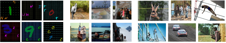
Figure 3: Datasets used for evaluation: Biased MNIST (left), COCO-on-Places (center), Biased Action Recognition (BAR) (right).

As the two loss gradients may conflict, we use a form of gradient surgery used in multi-task learning called projecting conflicting gradients (PCGrad) [47], whereby the gradient of one loss is projected onto the normal plane of the other when the gradients have negative cosine similarly. For each sample in each mini-batch, gradients for losses $(L_{s},L)$ are computed. If there is destructive interference, one gradient is selected at random and projected onto the normal plane of the other. In the case of constructive interference, both gradients are combined as usual. The cumulative update to the weights is then averaged over the batch. An ablation study showing experimental support for the use of gradient surgery is shown in Table 5.

3.4 Related Observations

Sharpening posterior estimates allows the network to first learn all features unhindered, then implicitly adjusts the weighting of those features with respect to the final task. The motivation for this novel approach stems from two main observations.

Addressing simplicity bias. Firstly, deep neural networks trained with empirical risk minimization (ERM) prefer simple solutions, tending to rely on spurious correlations especially when they are easier to learn than the core features. This has been referred to as simplicity bias [33]. Every bias mitigation method attempts to inform the model when it should rely on more complex predictive features versus when a simpler explanation is preferable. In literature, this has been addressed by either (1) selectively modifying the learned representations post-training [32, 13], or (2) guiding the network to selectively learn un-biased representations to begin with [27, 23, 29, 35, 36].

Posterior estimate sharpening falls in the first category, an implicitly-guided re-weighting of the classification head. It constrains the complexity of the model, not unlike OccamNets [35] which does so architecturally. Furthermore, sharpening is less prone to overfitting to minority samples as unlike [36, 10, 21, 12], it is not directly equivalent to up-weighting samples, focusing rather on feature weighting. The sharpening procedure addresses simplicity bias by relying on uncertainty estimates to inform when simpler solutions are not preferable, because they result in high uncertainties for bias-conflicting samples.

Adjusting Bayesian posteriors. Secondly, artificially tampering with posteriors of Bayesian deep neural networks is not a foreign concept. As presented by Wenzel et al. [45], the true Bayesian posteriors of deep neural networks are rarely used in practice. Rather, tempered or cold posteriors are widely found to perform better. Tempered posteriors are equivalent to over-counting the data by a factor of $1/T$ for temperature scalar $T$ and re-scaling the prior to $p(\boldsymbol{\theta})^{1/T}$. In contrast, the true Bayes posterior corresponding to $T=1$ usually gives sub-optimal performance.

We note, however, that our proposed sharpening procedure is applied only to the estimated posterior derived from MC sampling, not to the true Bayes posterior. The MC samples provide a finite, numerical handle on model inference. Furthermore, running the sharpening procedure with a sampling size $M$ of up to 20 indicates that increasing the MC sample size for a more accurate posterior estimate has negligible impact on the de-biasing.

4 Experiments

4.1 Datasets

Following the benchmarks established by Shreshtha et al. in  [35], we experiment on three datasets for visual bias mitigation shown in Figure 3. Biased MNIST [34] introduces color, texture, scale, and contextual biases into a 5 x 5 grid of cells, one or more of which contain one of the target MNIST 10 digits. With $p_{bias}=0.95$, each digit co-occurs 95% with each bias source. The test set is unbiased with a 50K/10K/10K train/val/test split. COCO-on-Places [1] spuriously correlates Places backgrounds with COCO object foregrounds. Most zebras, for example, appear in front of a desert, and most horses in front of a snowy landscape. Three test sets are provided: 1) biased backgrounds, matching the correlations present in the training set, 2) unseen backgrounds, including seen objects placed on new backgrounds unseen during training, and 3) seen but unbiased backgrounds. COCO-on-Places has a 7200/900/900 train/val/test split and 9 classes. Finally, Biased Action Recognition (BAR) [27] includes manually selected real-world images of action-background pairs, where the backgrounds are correlated to the action; e.g., most characters in the “climbing" class are climbing snowy mountains, and more rarely climb other objects such as buildings, structures, etc. BAR is the smallest dataset with a 1641/300/654 train/val/test split  and 6 target classes.

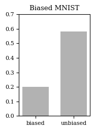
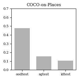
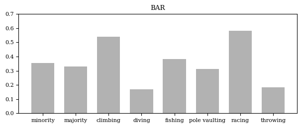
Figure 4: Mean uncertainties for subgroups of each test dataset, showing bias-induced discrepancies, but also increased uncertainties arising from a variety of other sources, some of which may be unintentional bias present in the data.

4.2 Group Epistemic Uncertainties

Unlike Biased-Synbols where the bias variable and its effect on model uncertainty can be observed and controlled in isolation, our benchmark datasets are significantly more complex. Bias-inducing features co-occur, but not always on the same samples (Biased MNIST). Classes can be severely imbalanced (BAR contains only 163 fishing images compared to its largest class of 520 images). Furthermore, both COCO and BAR exhibit intra-class diversity; the “racing" category includes bikes, motorcycles, runners, and a wide variety of vehicles, and COCO objects occur with different angles and coloring. This diversity also introduces bias into the dataset, albeit unintentional and unaccounted for. The mean group sample uncertainties extracted from Bayesian ResNet18 models trained on each dataset reflect this as well, as shown in Figure 4.

While this entangled experimental setup makes evaluation of the impact of de-biasing methods more difficult, the scenario is certainly realistic given the state of real-world visual datasets. Instead of explicitly disentangling the bias sources, sharpening trusts that the posterior adequately expresses its own shortages in information. Thus, sharpening considers class imbalance, intra-class diversity, unintentional biases, and known biases simultaneously.

4.3 Training and Inference

Optimal parameters for cSG-MCMC are determined via grid search for initial step sizes {0.01 0.05, 0.1, 0.5}, cycle lengths {150, 200, 300, 400, 500, 600, 700}, and Gaussian noise control parameter $\alpha\in$ {0.1, 0.3, 0.5, 0.7}. We fixed each schedule to 2 cycles and 3 moments sampled per sampling phase. Batch sizes for the baseline Bayesian models were fixed at 128 for training, and 64 for the sharpening procedure due to memory constraints (32 for BAR due to larger image size). Validation accuracy was used to determine stopping points and optimal hyper-parameters for both baseline Bayesian models and the sharpening procedure. Training took place on several IBM Power 9 dual-CPU nodes with 4 NVIDIA V100 GPUs. We refer readers to the Appendix for the optimal parameters for all experiments.

Following methodology reported in [35], we reduce the kernel size of the first convolutional layer of ResNet18 from 7 to 3 for COCO due to the small image size (64 x 64). We also initialize the priors for the BAR Bayesian ResNet18 models using the weights from a deterministic ResNet18 trained on an ImageNet subset of 100 classes.

The sharpening procedure requires keeping a handle on each Monte Carlo sample from $p(\boldsymbol{\theta}\mid D,\boldsymbol{x})$, and back-propagating on each of these samples for every iteration. Thus, the procedure has time complexity of $O(M\cdot N\cdot K)$ for $M$ posterior samples, $K$ multiplication operations as required for the network architecture, and $N$ iterations, versus $O(N\cdot K)$ for a deterministic network.

Table 1: Unbiased test set accuracies comparing Bay-ResNet against current debiasing methods. First, second and third best results are formatted.

Architecture+Method	Biased MNIST	COCO	BAR
Explicit method results
ResNet+UpWt	37.7 $\pm$ 1.6	35.2 $\pm$ 0.4	51.1 $\pm$ 1.9
ResNet+gDRO [30]	19.2 $\pm$ 0.9	35.3 $\pm 0.1$	38.7 $\pm$2.2
ResNet+PGI [1]	48.6 $\pm$ 0.7	42.7 $\pm$ 0.6	53.6 $\pm$0.9
Implicit method results
ResNet+ERM	36.8 $\pm$0.7	35.6 $\pm$ 1.0	51.3 $\pm$1.9
ResNet+SD [29]	37.1 $\pm$ 1.0	35.4 $\pm$ 0.5	51.3 $\pm$2.3
OccamResNet [35]	65.0 $\pm 1.0$	43.4 $\pm$ 1.0	52.6  $\pm$1.9
BayResNet+EpiWt [36]	34.4 $\pm 1.1$	34.4 $\pm$ 0.8	52.1 $\pm$1.5
BayResNet+Sharpen	38.6 $\pm$0.6	34.9 $\pm$0.6	53.9 $\pm$0.7

Table 2: Overall and per-class accuracies on BAR, showing large discrepancies in performance across methods and classes.

Methods	Overall	Climbing	Diving	Fishing	Pole Vaulting	Racing	Throwing
Explicit method results
ResNet+UpWt	51.1 $\pm 1.9$	61.7 $\pm 13.2$	43.9 $\pm 5.8$	42.3 $\pm 8.3$	52.3 $\pm 7.4$	67.9 $\pm 6.7$	28.2 $\pm 12.8$
ResNet+gDRO [30]	38.7 $\pm 2.2$	49.5 $\pm 8.5$	40.3 $\pm 8.4$	44.0 $\pm 10.4$	39.9 $\pm 7.1$	41.7 $\pm 4.0$	13.5 $\pm 5.9$
ResNet+PGI [1]	53.6 $\pm 0.9$	61.2 $\pm 10.4$	38.4 $\pm 4.1$	42.9 $\pm 8.4$	73.3 $\pm 3.7$	68.9 $\pm 5.9$	23.5 $\pm 1.9$
OccamResNet+UpWt	52.2 $\pm 1.4$	57.9 $\pm 1.8$	35.7 $\pm 7.5$	51.8 $\pm 11.2$	64.3 $\pm 8.8$	71.8 $\pm 3.8$	27.4 $\pm 3.5$
OccamResNet+gDRO [30]	52.9 $\pm 0.8$	51.2 $\pm 9.6$	42.8 $\pm 8.2$	52.3 $\pm 5.1$	63.5 $\pm 7.3$	74.2 $\pm 5.2$	25.3 $\pm 4.5$
OccamResNet+PGI [1]	55.9 $\pm 0.7$	64.2 $\pm 5.1$	52.3 $\pm 6.4$	51.4 $\pm 8.3$	64.4 $\pm 4.1$	70.9 $\pm 8.1$	18.6 $\pm 6.8$
Implicit method results
ResNet+ERM	51.3 $\pm 1.9$	69.5 $\pm 7.5$	29.2 $\pm 1.8$	39.9 $\pm 16.2$	55.5 $\pm 6.4$	75.6 $\pm 5.6$	31.8 $\pm 4.3$
ResNet+SD [29]	51.3 $\pm 2.3$	62.1 $\pm 7.5$	35.8 $\pm 2.0$	51.2 $\pm 6.4$	62.4 $\pm 9.2$	71.6 $\pm 10.0$	18.5 $\pm 6.7$
OccamResNet [30]	52.6 $\pm 1.9$	59.3 $\pm 3.8$	42.3 $\pm 7.5$	44.6 $\pm 14.9$	60.5 $\pm 8.6$	74.1 $\pm 7.2$	22.1 $\pm 3.9$
OccamResNet+SD [29]	52.3 $\pm 2.4$	56.4 $\pm 6.8$	34.3 $\pm 5.8$	55.4 $\pm 7.4$	69.1 $\pm 4.9$	72.9 $\pm 4.2$	21.8 $\pm 2.1$
BayResNet	52.7 $\pm 2.6$	71.1 $\pm 2.7$	28.3 $\pm 10.3$	54.8 $\pm 8.2$	54.2 $\pm 3.3$	78.0 $\pm 3.9$	31.8 $\pm 2.6$
BayResNet+EpiWt [36]	52.1 $\pm 1.6$	67.9 $\pm 2.2$	27.9 $\pm 5.1$	51.6 $\pm 5.4$	59.8 $\pm 3.5$	76.2 $\pm 0.4$	30.0 $\pm 2.9$
BayResNet+Sharpen	53.9 $\pm 0.7$	72.1 $\pm 2.0$	32.1 $\pm 3.2$	59.5 $\pm 2.3$	52.7 $\pm 2.7$	79.6 $\pm 0.7$	32.6 $\pm 2.9$

5 Results and Discussion

Table 3: Accuracies on all three test splits of COCO-on-Places: biased backgrounds (Bgs), unseen backgrounds, and seen but unbiased backgrounds.

Architecture+Method	Biased Bgs	Unseen Bgs	Seen, but Unbiased Bgs
Explicit method results
ResNet+PGI [1]	77.5 $\pm$0.6	52.8 $\pm$0.7	42.7 $\pm$0.6
OccamResNet+PGI [1]	82.8 $\pm$0.6	55.3 $\pm$1.3	43.6 $\pm$0.6
Implicit method results
ResNet+ERM	84.9 $\pm$ 0.5	53.2 $\pm$0.7	35.6 $\pm$1.0
OccamResNet [35]	84.0 $\pm$1.0	55.8 $\pm$1.2	43.4 $\pm$1.0
BayResNet	84.3 $\pm$0.4	49.7 $\pm$1.3	33.0 $\pm$0.2
BayResNet+EpiWt [36]	85.8 $\pm$0.1	50.3 $\pm$1.1	34.4 $\pm$0.8
BayResNet+Sharpen	85.6 $\pm$0.6	51.2 $\pm$0.2	34.9 $\pm$0.6

Table 4: Accuracies on majority (maj)/minority (min) groups and bias-induced accuracy gaps for each bias variable in BiasedMNIST ($p_{bias}=0.95$). Smallest accuracy gaps for each bias variable are in bold.

Architecture+Method		Digit Scale	Digit Color	Texture	Texture Color	Letter	Letter Color
	Test Acc.	maj/min ($\Delta$)	maj/min ($\Delta$)	maj/min ($\Delta$)	maj/min ($\Delta$)	maj/min ($\Delta$)	maj/min ($\Delta$)
ResNet+ERM	36.8	87.2/31.3 (55.9)	78.5/32.1 (46.4)	76.1/32.4 (43.7)	41.9/36.3 (5.6)	46.7/35.7 (11.0)	45.7/35.9 (9.8)
BayResNet+Sharpen	38.6	89.9/32.2 (57.7)	82.6/32.9 (49.7)	61.3/35.3 (26.0)	40.0/37.8 (2.2)	44.2/37.3 (6.9)	45.2/37.2 (8.0)

Table 5: Ablation study on sharpening procedure loss functions and their performance on the most difficult test sets for each dataset. Validation accuracy was used for optimization in each case.

Sharpening Loss	Biased MNIST	COCO	BAR
$L_{s}$	34.8 $\pm$ 2.1	33.3 $\pm$ 1.4	53.5 $\pm$1.0
$L+k\cdot L_{s}$	33.4 $\pm$0.2	32.3 $\pm$ 0.3	53.2 $\pm$0.4
$\textup{PCGrad}(L_{s},L)$	38.6 $\pm$0.5	34.9 $\pm$1.2	53.9 $\pm$0.7

For a fair comparison against prior reported results on these datasets, we use a ResNet18 throughout the experiments. We compare against several explicit and implicit mitigation methods, separated in each table: UpWt, gDRO, and PGI for explicit approaches, and the baseline ERM, SD and OccamNet for implicits. We also include EpiWt, another implicit method, due to its similarity to our approach in leveraging the epistemic uncertainties of a Bayesian neural network. We consider two baselines: (1) empirical risk minimization (ERM) of a deterministic ResNet18, and (2) a Bayesian ResNet18, both trained with normal cross entropy loss and no bias mitigation. The sharpening procedure gives competitive results on BAR, and comparable performance on Biased MNIST (Table 1).

We observe poorer performance on the COCO dataset. Posterior estimate sharpening always increases model fairness when compared to its baseline Bayesian starting point. As demonstrated in Table 3, the Bayesian ResNet struggles with both the out-of-distribution and unbiased background test sets, with differences of -3.5% and -2.6% respectively compared to the deterministic ERM baseline. Building on the BayResNet, the sharpening thus starts with a more unfair model than methods based on a deterministic ERM model, giving it a distinct disadvantage. Assuming the discrepancy in performance is somewhat due to the stochastic nature of the network, BayResNet+EpiWt would also have a disadvantage but does better on the biased test set than BayResNet+Sharpen; nonetheless, as is consistent across datasets, BayResNet+Sharpen still does better than BayResNet+EpiWt on the two unbiased test sets.

Regardless, this highlights a weakness of the sharpening approach. We consider the vast topic of comparing the predictive performances of deterministic and Bayesian neural networks out of the scope of this paper, but acknowledge that Bayesian neural networks can struggle to match deterministic benchmarks, which directly affects the sharpening method. We weigh these sacrifices in performance against the added benefit of quantified prediction uncertainty estimates, which deterministic models fail to communicate altogether.

BAR is a counterexample, where the Bayesian baseline outperforms or does at least as well as the deterministic one across class groups. The most realistic and complex dataset of the three, BAR is neither texturally simple like Biased MNIST nor synthetically created and low-resolution like COCO-on-Places. The posterior estimate sharpening method performs well on BAR (Table 2), especially considering the large discrepancy in performances across classes and methods. Notably, while various methods do well in two or three classes, BayResNet+Sharpen has good performance across the majority of classes (5/7 classes). For this dataset, perhaps because of its ability to regularize despite the small dataset size and substantial intra-class diversity, the baseline BayResNet provides a strong starting point for the sharpening method.

Table 4 shows the majority/minority group accuracies and bias-induced accuracy gap for the six bias variables in Biased MNIST. Compared to the baseline ERM, the sharpened model decreases the accuracy gaps between majority and minority groups across the dataset for 4 out of 6 of the biases (texture, texture color, letter, and letter color). While BayResNet+Sharpen results on Biased MNIST are not as competitive, results demonstrate that the sharpening objective aims at increasing model fairness rather than simply rewarding accuracy gains on the majority groups.

We consider the impact of PCGrad on the multi-task loss in the ablation study shown in Table 5. For weighted loss $L+k\cdot L_{s}$, scalar weight $k$ is chosen using a grid search in range $k=2$ to $k=10$ with optimal $k$ being in range 3 to 5 for all datasets with negligible impact for $k<3$ and declining accuracy (biased and unbiased sets) for values $k>5$; this loss simply adds the two losses together regardless of conflict, with a fixed weighting term across all samples.

Finally, uncertainty distributions across training sets do not collapse under PCGrad sharpening, so sample uncertainty estimates extracted at inference time may still be useful for triage or other purposes in high-risk scenarios.

6 Conclusion

The visual datasets heavily relied on by today’s deep neural networks are complex, feature-dense, and full of unidentified biases and spurious correlations. While no single bias mitigation method has thus far been unilaterally successful, a wide variety of ideas in recent literature make promising advances in both explicit and implicit mitigation.

Our posterior estimate sharpening method adds to this body of work by implicitly exploiting the relationship between minority samples and epistemic uncertainties. We have demonstrated competitive performance on one benchmark, and comparable results on another. Further exploration is required to better understand when and why Bayesian neural networks struggle with respect to deterministic networks within the context of bias mitigation, and why the performances of mitigation methods vary across datasets. This perhaps calls for a better disentangling of features and correlations within training and test datasets used for evaluation, which we leave for future consideration.

7 Acknowledgements

The first author is a recipient of an Ezra Rabin Scholarship. Training was carried out on Bede, a facility of the N8 Centre of Excellence in Computationally Intensive Research (N8 CIR) . We would like to acknowledge the respective authors for their publicly available code for cSG-MCMC , network dissection , PCGrad [39], and OccamNets  from which we have modified code for our work. We thank Robik Shrestha for kindly providing the checkpoint for the ResNet18 trained on the ImageNet-100 subset, which was used as the prior for the BAR models. Finally, special thanks to Jose Sosa and Mohammed Alghamdi from the School of Computing’s Computer Vision Group for critical feedback and many great discussions.

References

- [1] Faruk Ahmed, Yoshua Bengio, Harm Van Seijen, and Aaron Courville. Systematic generalisation with group invariant predictions. In International Conference on Learning Representations, 2021.
- [2] Junaid Ali, Preethi Lahoti, and Krishna P Gummadi. Accounting for model uncertainty in algorithmic discrimination. In Proceedings of the 2021 AAAI/ACM Conference on AI, Ethics, and Society, pages 336–345, 2021.
- [3] Mohsan Alvi, Andrew Zisserman, and Christoffer Nellåker. Turning a blind eye: Explicit removal of biases and variation from deep neural network embeddings. In Proceedings of the European Conference on Computer Vision (ECCV) Workshops, pages 0–0, 2018.
- [4] Alexander Amini, Ava P Soleimany, Wilko Schwarting, Sangeeta N Bhatia, and Daniela Rus. Uncovering and mitigating algorithmic bias through learned latent structure. In Proceedings of the 2019 AAAI/ACM Conference on AI, Ethics, and Society, pages 289–295, 2019.
- [5] Hyojin Bahng, Sanghyuk Chun, Sangdoo Yun, Jaegul Choo, and Seong Joon Oh. Learning de-biased representations with biased representations. In International Conference on Machine Learning, pages 528–539. PMLR, 2020.
- [6] David Bau, Bolei Zhou, Aditya Khosla, Aude Oliva, and Antonio Torralba. Network dissection: Quantifying interpretability of deep visual representations. In Proceedings of the IEEE conference on computer vision and pattern recognition, pages 6541–6549, 2017.
- [7] Frédéric Branchaud-Charron, Parmida Atighehchian, Pau Rodríguez, Grace Abuhamad, and Alexandre Lacoste. Can active learning preemptively mitigate fairness issues? arXiv preprint arXiv:2104.06879, 2021.
- [8] Joy Buolamwini and Timnit Gebru. Gender shades: Intersectional accuracy disparities in commercial gender classification. In Conference on fairness, accountability and transparency, pages 77–91. PMLR, 2018.
- [9] Robert Challen, Joshua Denny, Martin Pitt, Luke Gompels, Tom Edwards, and Krasimira Tsaneva-Atanasova. Artificial intelligence, bias and clinical safety. BMJ Quality & Safety, 28(3):231–237, 2019.
- [10] Nitesh V Chawla, Kevin W Bowyer, Lawrence O Hall, and W Philip Kegelmeyer. Smote: synthetic minority over-sampling technique. Journal of artificial intelligence research, 16:321–357, 2002.
- [11] Alexandra Chouldechova, Diana Benavides-Prado, Oleksandr Fialko, and Rhema Vaithianathan. A case study of algorithm-assisted decision making in child maltreatment hotline screening decisions. In Conference on Fairness, Accountability and Transparency, pages 134–148. PMLR, 2018.
- [12] Yin Cui, Menglin Jia, Tsung-Yi Lin, Yang Song, and Serge Belongie. Class-balanced loss based on effective number of samples. In Proceedings of the IEEE/CVF conference on computer vision and pattern recognition, pages 9268–9277, 2019.
- [13] Mengnan Du, Subhabrata Mukherjee, Guanchu Wang, Ruixiang Tang, Ahmed Awadallah, and Xia Hu. Fairness via representation neutralization. Advances in Neural Information Processing Systems, 34:12091–12103, 2021.
- [14] Cynthia Dwork, Moritz Hardt, Toniann Pitassi, Omer Reingold, and Richard Zemel. Fairness through awareness. In Proceedings of the 3rd innovations in theoretical computer science conference, pages 214–226, 2012.
- [15] Yarin Gal, Riashat Islam, and Zoubin Ghahramani. Deep bayesian active learning with image data. In International Conference on Machine Learning, pages 1183–1192. PMLR, 2017.
- [16] Robert Geirhos, Patricia Rubisch, Claudio Michaelis, Matthias Bethge, Felix A Wichmann, and Wieland Brendel. Imagenet-trained cnns are biased towards texture; increasing shape bias improves accuracy and robustness. arXiv preprint arXiv:1811.12231, 2018.
- [17] Asma Ghandeharioun, Brian Eoff, Brendan Jou, and Rosalind Picard. Characterizing sources of uncertainty to proxy calibration and disambiguate annotator and data bias. In 2019 IEEE/CVF International Conference on Computer Vision Workshop (ICCVW), pages 4202–4206. IEEE, 2019.
- [18] Melissa Hall, Laurens van der Maaten, Laura Gustafson, and Aaron Adcock. A systematic study of bias amplification. arXiv preprint arXiv:2201.11706, 2022.
- [19] Haibo He, Yang Bai, Edwardo A Garcia, and Shutao Li. Adasyn: Adaptive synthetic sampling approach for imbalanced learning. In 2008 IEEE international joint conference on neural networks (IEEE world congress on computational intelligence), pages 1322–1328. IEEE, 2008.
- [20] Laurent Valentin Jospin, Hamid Laga, Farid Boussaid, Wray Buntine, and Mohammed Bennamoun. Hands-on bayesian neural networks—a tutorial for deep learning users. IEEE Computational Intelligence Magazine, 17(2):29–48, 2022.
- [21] Faisal Kamiran and Toon Calders. Data preprocessing techniques for classification without discrimination. Knowledge and information systems, 33(1):1–33, 2012.
- [22] Salman Khan, Munawar Hayat, Syed Waqas Zamir, Jianbing Shen, and Ling Shao. Striking the right balance with uncertainty. In Proceedings of the IEEE/CVF Conference on Computer Vision and Pattern Recognition, pages 103–112, 2019.
- [23] Nayeong Kim, Sehyun Hwang, Sungsoo Ahn, Jaesik Park, and Suha Kwak. Learning debiased classifier with biased committee. arXiv preprint arXiv:2206.10843, 2022.
- [24] Agustinus Kristiadi, Matthias Hein, and Philipp Hennig. Being bayesian, even just a bit, fixes overconfidence in relu networks. In International conference on machine learning, pages 5436–5446. PMLR, 2020.
- [25] Alexandre Lacoste, Pau Rodríguez López, Frédéric Branchaud-Charron, Parmida Atighehchian, Massimo Caccia, Issam Hadj Laradji, Alexandre Drouin, Matthew Craddock, Laurent Charlin, and David Vázquez. Synbols: Probing learning algorithms with synthetic datasets. Advances in Neural Information Processing Systems, 33:134–146, 2020.
- [26] Ninareh Mehrabi, Fred Morstatter, Nripsuta Saxena, Kristina Lerman, and Aram Galstyan. A survey on bias and fairness in machine learning. ACM Computing Surveys (CSUR), 54(6):1–35, 2021.
- [27] Junhyun Nam, Hyuntak Cha, Sungsoo Ahn, Jaeho Lee, and Jinwoo Shin. Learning from failure: De-biasing classifier from biased classifier. Advances in Neural Information Processing Systems, 33:20673–20684, 2020.
- [28] Peter A Noseworthy, Zachi I Attia, LaPrincess C Brewer, Sharonne N Hayes, Xiaoxi Yao, Suraj Kapa, Paul A Friedman, and Francisco Lopez-Jimenez. Assessing and mitigating bias in medical artificial intelligence: the effects of race and ethnicity on a deep learning model for ecg analysis. Circulation: Arrhythmia and Electrophysiology, 13(3):e007988, 2020.
- [29] Mohammad Pezeshki, Oumar Kaba, Yoshua Bengio, Aaron C Courville, Doina Precup, and Guillaume Lajoie. Gradient starvation: A learning proclivity in neural networks. Advances in Neural Information Processing Systems, 34:1256–1272, 2021.
- [30] Shiori Sagawa, Pang Wei Koh, Tatsunori B Hashimoto, and Percy Liang. Distributionally robust neural networks for group shifts: On the importance of regularization for worst-case generalization. arXiv preprint arXiv:1911.08731, 2019.
- [31] Victor Sanh, Thomas Wolf, Yonatan Belinkov, and Alexander M Rush. Learning from others’ mistakes: Avoiding dataset biases without modeling them. arXiv preprint arXiv:2012.01300, 2020.
- [32] Shibani Santurkar, Dimitris Tsipras, Mahalaxmi Elango, David Bau, Antonio Torralba, and Aleksander Madry. Editing a classifier by rewriting its prediction rules. Advances in Neural Information Processing Systems, 34:23359–23373, 2021.
- [33] Harshay Shah, Kaustav Tamuly, Aditi Raghunathan, Prateek Jain, and Praneeth Netrapalli. The pitfalls of simplicity bias in neural networks. Advances in Neural Information Processing Systems, 33:9573–9585, 2020.
- [34] Robik Shrestha, Kushal Kafle, and Christopher Kanan. An investigation of critical issues in bias mitigation techniques. In Proceedings of the IEEE/CVF Winter Conference on Applications of Computer Vision, pages 1943–1954, 2022.
- [35] Robik Shrestha, Kushal Kafle, and Christopher Kanan. Occamnets: Mitigating dataset bias by favoring simpler hypotheses. In Computer Vision–ECCV 2022: 17th European Conference, Tel Aviv, Israel, October 23–27, 2022, Proceedings, Part XX, pages 702–721. Springer, 2022.
- [36] Rebecca S Stone, Nishant Ravikumar, Andrew J Bulpitt, and David C Hogg. Epistemic uncertainty-weighted loss for visual bias mitigation. In Proceedings of the IEEE/CVF Conference on Computer Vision and Pattern Recognition, pages 2898–2905, 2022.
- [37] Enzo Tartaglione, Carlo Alberto Barbano, and Marco Grangetto. End: Entangling and disentangling deep representations for bias correction. In Proceedings of the IEEE/CVF Conference on Computer Vision and Pattern Recognition, pages 13508–13517, 2021.
- [38] William Thong and Cees GM Snoek. Feature and label embedding spaces matter in addressing image classifier bias. arXiv preprint arXiv:2110.14336, 2021.
- [39] Wei-Cheng Tseng. Weichengtseng/pytorch-pcgrad, 2020.
- [40] Christina Wadsworth, Francesca Vera, and Chris Piech. Achieving fairness through adversarial learning: an application to recidivism prediction. arXiv preprint arXiv:1807.00199, 2018.
- [41] Mei Wang and Weihong Deng. Mitigating bias in face recognition using skewness-aware reinforcement learning. In Proceedings of the IEEE/CVF conference on computer vision and pattern recognition, pages 9322–9331, 2020.
- [42] Zeyu Wang, Klint Qinami, Ioannis Christos Karakozis, Kyle Genova, Prem Nair, Kenji Hata, and Olga Russakovsky. Towards fairness in visual recognition: Effective strategies for bias mitigation. In Proceedings of the IEEE/CVF conference on computer vision and pattern recognition, pages 8919–8928, 2020.
- [43] Gary M Weiss, Kate McCarthy, and Bibi Zabar. Cost-sensitive learning vs. sampling: Which is best for handling unbalanced classes with unequal error costs? Dmin, 7(35-41):24, 2007.
- [44] Max Welling and Yee W Teh. Bayesian learning via stochastic gradient langevin dynamics. In Proceedings of the 28th international conference on machine learning (ICML-11), pages 681–688. Citeseer, 2011.
- [45] Florian Wenzel, Kevin Roth, Bastiaan S Veeling, Jakub Świątkowski, Linh Tran, Stephan Mandt, Jasper Snoek, Tim Salimans, Rodolphe Jenatton, and Sebastian Nowozin. How good is the bayes posterior in deep neural networks really? arXiv preprint arXiv:2002.02405, 2020.
- [46] Xingkun Xu, Yuge Huang, Pengcheng Shen, Shaoxin Li, Jilin Li, Feiyue Huang, Yong Li, and Zhen Cui. Consistent instance false positive improves fairness in face recognition. In Proceedings of the IEEE/CVF Conference on Computer Vision and Pattern Recognition, pages 578–586, 2021.
- [47] Tianhe Yu, Saurabh Kumar, Abhishek Gupta, Sergey Levine, Karol Hausman, and Chelsea Finn. Gradient surgery for multi-task learning. Advances in Neural Information Processing Systems, 33:5824–5836, 2020.
- [48] Brian Hu Zhang, Blake Lemoine, and Margaret Mitchell. Mitigating unwanted biases with adversarial learning. In Proceedings of the 2018 AAAI/ACM Conference on AI, Ethics, and Society, pages 335–340, 2018.
- [49] Ruqi Zhang, Chunyuan Li, Jianyi Zhang, Changyou Chen, and Andrew Gordon Wilson. Cyclical stochastic gradient mcmc for bayesian deep learning. arXiv preprint arXiv:1902.03932, 2019.
- [50] Jieyu Zhao, Tianlu Wang, Mark Yatskar, Vicente Ordonez, and Kai-Wei Chang. Men also like shopping: Reducing gender bias amplification using corpus-level constraints. In EMNLP, 2017.