HoloDiffusion: Training a 3D Diffusion Model using 2D Images

Abstract

Diffusion models have emerged as the best approach for generative modeling of 2D images. Part of their success is due to the possibility of training them on millions if not billions of images with a stable learning objective. However, extending these models to 3D remains difficult for two reasons. First, finding a large quantity of 3D training data is much more complex than for 2D images. Second, while it is conceptually trivial to extend the models to operate on 3D rather than 2D grids, the associated cubic growth in memory and compute complexity makes this infeasible. We address the first challenge by introducing a new diffusion setup that can be trained, end-to-end, with only posed 2D images for supervision; and the second challenge by proposing an image formation model that decouples model memory from spatial memory. We evaluate our method on real-world data, using the CO3D dataset which has not been used to train 3D generative models before. We show that our diffusion models are scalable, train robustly, and are competitive in terms of sample quality and fidelity to existing approaches for 3D generative modeling.

1 Introduction

Diffusion models have rapidly emerged as formidable generative models for images, replacing others (e.g., VAEs, GANs) for a range of applications, including image colorization [51], image editing [39], and image synthesis [23, 9]. These models explicitly optimize the likelihood of the training samples, can be trained on millions if not billions of images, and have been shown to capture the underlying model distribution better [9] than previous alternatives.

A natural next step is to bring diffusion models to 3D data. Compared to 2D images, 3D models facilitate direct manipulation of the generated content, result in perfect view consistency across different cameras, and allow object placement using direct handles. However, learning 3D diffusion models is hindered by the lack of a sufficient volume of 3D data for training. A further question is the choice of representation for the 3D data itself (e.g., voxels, point clouds, meshes, occupancy grids, etc.). Researchers have proposed 3D-aware diffusion models for point clouds [37], volumetric shape data using wavelet features [24] and novel view synthesis [66]. They have also proposed to distill a pretrained 2D diffusion model to generate neural radiance fields of 3D objects [49, 34]. However, a diffusion-based 3D generator model trained using only 2D image for supervision is not available yet.

In this paper, we contribute HoloDiffusion, the first unconditional 3D diffusion model that can be trained with only real posed 2D images. By posed, we mean different views of the same object with known cameras, for example, obtained by means of structure from motion [53].

We make two main technical contributions: (i) We propose a new 3D model that uses a hybrid explicit-implicit feature grid. The grid can be rendered to produce images from any desired viewpoint and, since the features are defined in 3D space, the rendered images are consistent across different viewpoints. Compared to utilizing an explicit density grid, the feature representation allows for a lower resolution grid. The latter leads to an easier estimation of the probability density due to a smaller number of variables. Furthermore, the resolution of the grid can be decoupled from the resolution of the rendered images. (ii) We design a new diffusion method that can learn a distribution over such 3D feature grids while only using 2D images for supervision. Specifically, we first generate intermediate 3D-aware features conditioned only on the input posed images. Then, following the standard diffusion model learning, we add noise to this intermediate representation and train a denoising 3D UNet to remove the noise. We apply the denoising loss as photometric error between the rendered images and the Ground-Truth training images. The key advantage of this approach is that it enables training of the 3D diffusion model from 2D images, which are abundant, sidestepping the difficult problem of procuring a huge dataset of 3D models for training.

We train and evaluate our method on the Co3Dv2 [50] dataset where HoloDiffusion outperforms existing alternatives both qualitatively and quantitatively.

2 Related Work

2.1 Image-conditioned 3D Reconstruction

Neural and differentiable rendering.

Neural rendering [60] is a class of algorithms that partially or entirely use neural networks to approximate the light transport equation.

The 2D versions of neural rendering include variants of pix2pix [25], deferred neural rendering [61], and their follow-up works. The common theme in all these methods is that a post-processor neural network (usually a CNN) maps neural feature images into photorealistic RGB images.

The 3D versions of neural rendering have recently been popularized by NeRF [40], which uses a Multi Layer Perceptron (MLP) to model the parameters of the 3D scene (radiance and occupancy) and a physically-based rendering procedure (Emission-Absorption raymarching). NeRF solves the inverse rendering problem where, given many 2D images of a scene, the aim is to recover its 3D shape and appearance. The success of NeRF gave rise to many follow-up works [40, 1, 73, 2, 63]. While NeRF uses MLPs to represent the occupancy and radiance of the underlying scene, different representations were explored in [35, 7, 71, 59, 42, 64, 14, 29].

Figure 2: Method overview. Our HoloDiffusion takes as input video frames for category-specific videos $\{s^{i}\}$ and trains a diffusion-based generative model $\mathcal{D}_{\theta}$. The model is trained with only posed image supervision $\{(I_{j}^{i},P_{j}^{i})\}$, without access to 3D ground-truth. Once trained, the model can generate view-consistent results from novel camera locations. Please refer to Sec. 3 for details.

Few-view reconstruction.

In many cases, dense image supervision is unavailable, and one has to condition the reconstruction on a small number of scene views instead. Since 3D reconstruction from few-views is ambiguous, recent methods aid the reconstruction with 3D priors learned by observing many images of an object category. Works like CMR [27], C3DM [47], and UMR [33] learn to predict the parameters of a mesh by observing images of individual examples of the object category. DOVE [68] also predicts meshes, but additionally leverages stronger constraints provided by videos of the deformable objects.

Others [72, 19] aimed at learning to fit NeRF given only a small number of views; they do so by sampling image features at the 2D projections of the 3D ray samples. Later works [50, 65] have improved this formulation by using transformers to process the sampled features. Finally, ViewFormer [32] drops the rendering model and learns a fully implicit transformer-based new-view synthesizer. Recently, BANMo [70] reconstructed deformable objects with a signed distance function.

2.2 3D Generative Models

3D Generative advesarial networks.

Early 3D generative models leveraged adversarial learning [13] as the primary form of supervision. PlatonicGAN [18] learns to generate colored 3D shapes from an unstructured corpus of images belonging to the same category, by rendering a voxel grid from random viewpoints so that an adversarial discriminator cannot distinguish between the renders and natural images sampled from a large uncurated database. PrGAN [10] differs from PlatonicGAN by focusing only on rendering untextured 3D shapes. To deal with the large memory footprint of voxels, HoloGAN [43] adjusts PlatonicGAN by rendering a low-resolution 2D feature image of a coarse voxel grid, followed by a 2D convolutional decoder mapping the feature render to the final RGB image. The results are, however, not consistent with camera motion.

Inspired by the success of NeRF [41], GRAF [54] also trains in a data setting similar to PlatonicGAN [18] but, differently from PlatonicGAN, represents each generated scene with a neural radiance field. The GRAF pipeline was subsequently improved by PiGAN [6], leveraging a SIREN-based [56] architecture. Similar to HoloGAN, StyleNerf [15] first renders a radiance feature field followed by a convolutional super-resolution network. EG3D [5] further improves the pipeline by initially decoding a randomly sampled latent vector to a tri-plane representation followed by a NeRF-style rendering of a radiance field supported by the tri-plane. EpiGRAF [57] further improves upon the triplane-based 3D generation. GAUDI [3] also uses the tri-plane while building upon DeVries et. al. [8] which used a single plane representing the floor map of the indoor room scenes being generated.

Besides radiance fields, other shape representations have also been explored. While VoxGRAF [55] replaces the radiance field of GRAF with a sparse voxel grid, StyleSDF [48] employs signed distance fields, and Neural Volumes [35] propose a novel trilinearly-warped voxel grid. Wu et al. [69] differentiably render meshes and aid the adversarial learning with a set of constraints exploiting symmetry properties of the reconstructed categories. Recently, GET3D [11] differentiably converts an initial tri-plane representation to colored mesh, which is finally rendered.

The aforementioned approaches are trained solely by observing uncurated category-centric image collections without the need for any explicit 3D supervision in form of the ground truth 3D shape or camera pose. However, since the rendering function is non-smooth under camera motion, these methods can either successfully reconstruct image databases with a very small variation in camera poses (e.g., fronto-parallel scenes such as portrait photos of cat or human faces) or datasets with a well-defined distribution of camera intrinsics end extrinsics (e.g., synthetic datasets). We tackle the pose estimation problem by leveraging a dataset of category-centric videos each containing multiple views of the same object. Observing each object from a moving vantage point allows for estimating accurate scene-consistent camera poses that provide strong constraints.

While most approaches focus on generating shapes of isolated instances of object categories, GIRAFFE [46] and BlockGAN [44] extend GRAF and HoloGAN to reconstruct compositions of objects and their background. Alternative approaches focus on text-conditioned 3D shape generation [3, 26, 49], or learn [28] a generative model by observing a single self-similar scene.

3D diffusion models.

Diffusion models for 3D shape learning have been explored only very recently. Luo et al. [38] use full 3D supervision to learn a generative diffusion model of point clouds. In a concurrent effort, Watson et al. [67] learns a new-view synthesis function which, conditioned on a posed image of a scene, generates a new view of the scene from a specified target viewpoint. Differently from us, [67] do not employ an explicit image formation model which may lead to geometrical inconsistencies between generated viewpoints.

3 HoloDiffusion

We start by discussing the necessary background and notation on diffusion models in Sec. 3.1, and then we introduce our method in Sec. 3.2, Sec. 3.3, and Sec. 3.4.

3.1 Diffusion Models

Given $N$ i.i.d. samples $\{x^{i}\}_{i=1}^{N}$ from (an unknown) data distribution $p(x)$, the task of generative modeling is to find the parameters $\theta$ of a parametric model $p_{\theta}(x)$ that best approximate $p(x)$. Diffusion models are a class of likelihood-based models centered on the idea of defining a forward diffusion (noising) process $q(x_{t}|x_{t-1})$, for $t\in[0,T]$. The noising process converts the data samples into pure noise, i.e., $q(x_{T})\approx q(x_{T}|x_{T-1})=\mathcal{N}(0,I)$. The model then learns the reverse process $p(x_{t-1}|x_{t})$, which iteratively converts the noise samples back into data samples starting from the purely Gaussian sample $x_{T}$.

The Denoising Diffusion Probabilistic Model (DDPM) [22], in particular, defines the noising transitions using a Gaussian distribution, setting

$$q(x_{t}|x_{t-1}):=\mathcal{N}(x_{t};\sqrt{\alpha_{t}}x_{t-1},(1-\alpha_{t})I).$$ (1)

Samples can be easily drawn from this distribution by using the reparameterization trick:

$$x_{t}:=\sqrt{\alpha_{t}}x_{t-1}+\sqrt{1-\alpha_{t}}\epsilon~{}~{}~{}\text{where}~{}~{}~{}\epsilon\sim\mathcal{N}(0,I).$$ (2)

One similarly defines the reverse denoising step using a Gaussian distribution:

$$p_{\theta}(x_{t-1}|x_{t}):=\mathcal{N}(x_{t-1};\sqrt{\alpha_{t}}\mathcal{D}_{\theta}(x_{t},t),(1-\alpha_{t})I),$$ (3)

where, the $\mathcal{D}_{\theta}$ is the denoising network with learned parameters $\theta$. The sequence $\alpha_{t}$ defines the noise schedule as:

$$\alpha_{t}=1-\beta_{t},\quad\beta_{t}\in[0,1],\quad\text{s.t.~{}}\beta_{t}>\beta_{t-1}\forall t\in[0,T].$$ (4)

We use a linear time schedule with $T=1000$ steps.

The denoising must be applied iteratively for sampling the target distribution $p(x)$. However, for training the model we can draw samples $x_{t}$ directly from $q(x_{t}|x_{0})$ as:

$$x_{t}=\sqrt{\bar{\alpha}_{t}}x_{0}+\sqrt{1-\bar{\alpha}_{t}}\epsilon\quad\text{where, }\bar{\alpha}_{t}=\prod_{i=0}^{t}\alpha_{i}.$$ (5)

It is common to use the network $\mathcal{D}_{\theta}(x_{t},t)$ to predict the noise component $\epsilon$ instead of the signal component $x_{t-1}$ in eq. 2; which has the interpretation of modeling the score of the marginal distribution $q(x_{t})$ up to a scaled constant [22, 36]. Instead, we employ the “$x_{0}$-formulation” from eq. 3, which has recently been explored in the context of diffusion model distillation [52] and modeling of text-conditioned videos using diffusion [21]. The reasoning behind this design choice will become apparent later.

Training.

Training the “$x_{0}$-formulation” of a diffusion model $\mathcal{D}_{\theta}$ comprises minimizing the following loss:

$$\mathcal{L}=\|\mathcal{D}_{\theta}(x_{t},t)-x_{0}\|^{2},$$ (6)

encouraging $\mathcal{D}_{\theta}$ to denoise sample $x_{t}\sim\mathcal{N}(\sqrt{\bar{\alpha}_{t}}x_{0},(1-\bar{\alpha}_{t})I)$ to predict the clean sample $x_{0}$.

Sampling.

Once the denoising network $\mathcal{D}_{\theta}$ is trained, sampling can be done by first starting with pure noise, i.e., $x_{T}\sim\mathcal{N}(0,I)$, and then iteratively refining $T$ times using the network $\mathcal{D}_{\theta}$, which terminates with a sample from target data distribution $x_{0}\sim q(x_{0})=p(x)$:

$$x_{t-1}\sim\mathcal{N}(\sqrt{\bar{\alpha}_{t-1}}\mathcal{D}_{\theta}(x_{t},t),(1-\bar{\alpha}_{t-1})I).$$ (7)

3.2 Learning 3D Categories by Watching Videos

Training data.

The input to our learning procedure is a dataset of $N\in\mathbb{N}$ video sequences $\{s^{i}\}_{i=1}^{N}$, each depicting an instance of the same object category (e.g., car, carrot, teddy bear). Each video $s^{i}=(I^{i}_{j},P^{i}_{j})_{j=1}^{N_{\text{frames}}}$ comprises $N_{\text{frames}}$ pairs $(I^{i}_{j},P^{i}_{j})$, each consisting of an RGB image $I^{i}_{j}\in{}^{3\times H\times W}$ and its corresponding camera pose $P^{i}_{j}\in{}^{4\times 4}$, represented as a $4\times 4$ camera matrix.

Our goal is to train a generative model $p(V)$ where $V$ is a representation of the shape and appearance of a 3D object; furthermore, we aim to learn this distribution using only the 2D training videos $\{s^{i}\}_{i=1}^{N}$.

3D feature grids.

As 3D representation $V$ we pick 3D feature voxel grids $V\in{}^{d^{V}\times S\times S\times S}$ of size $S\in\mathbb{N}$ containing $d^{V}$-dimensional latent feature vectors. Given the voxel grid $V$ representing the object from a certain video $s$, we can reconstruct any frame $(I_{j},P_{j})\in s$ of the video as $I_{j}=r_{\zeta}(V,P_{j})$ by the means of the rendering function $r_{\zeta}(V,P_{j}):{}^{d^{V}\times S\times S\times S}\times{}^{4\times 4}\mapsto{}^{3\times H\times W}$, where $\zeta$ are the function parameters (see Sec. 3.4 for details).

Next, we discuss how to build a diffusion model for the distribution $p(V)$ of feature grids. One might attempt to directly apply the methodology of Sec. 3.1, setting $x=V$, but this does not work because we have no access to ground-truth feature grids $V$ for training; instead, these 3D models must be inferred from the available 2D videos while training. We solve this problem in the next section.

3.3 Bootstrapped Latent Diffusion Model

In this section, we show how to learn the distribution $p(V)$ of feature grids from the training videos $s$ alone. In what follows, we use the symbol $\mathcal{V}$ as a shorthand for $p(V)$.

The training videos provide RGB images $I$ and their corresponding camera poses $P$, but no sample feature grids $V$ from the target distribution $\mathcal{V}$. As a consequence, we also have no access to the noised samples $V_{t}\sim\mathcal{N}(\sqrt{\bar{\alpha}_{t}}V_{0},(1-\bar{\alpha}_{t})I)$ required to evaluate the denoising objective eq. 6 and thus learn a diffusion model.

To solve this issue, we introduce the BLDM (Bootstrapped Latent Diffusion Model). BLDM can learn the denoiser-cum-generator $\mathcal{D}_{\theta}$ given samples $\bar{V}\sim\mathcal{\bar{V}}$ from an auxiliary distribution $\mathcal{\bar{V}}$, which is closely related but not identical to the target distribution $\mathcal{V}$.

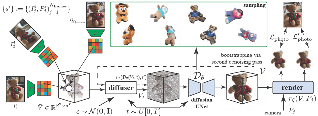
The auxiliary samples $\bar{V}$.

As shown in fig. 2, our idea is to obtain the auxiliary samples $\bar{V}$ as a (learnable) function of the corresponding training videos $s$. To this end, we use a design strongly inspired by Warp-Conditioned-Embedding (WCE) [19], which demonstrated compelling performance for learning 3D object categories. Specifically, given a training video $s$ containing frames $I_{j}$, we generate a grid $\bar{V}\in{}^{d^{V}\times S\times S\times S}$ of auxiliary features $\bar{V}_{:mno}\in[-1,1]^{d_{V}}$ by projecting the 3D coordinate $\mathbf{x}^{V}_{mno}$ of the each grid element $(m,n,o)$ to every video frame $I_{j}$, sampling corresponding 2D image features, and aggregating those into a single $d_{V}$-dimensional descriptor per grid element. The 2D image features are extracted by a trainable encoder (we use the ResNet-32 encoder [17]) $E$. This process is detailed in the supplementary material.

Auxiliary denoising diffusion objective.

The standard denoising diffusion loss eq. 6 is unavailable in our case because the data samples $V$ are unavailable. Instead, we leverage the “$x_{0}$-formulation” of diffusion to employ an alternative diffusion objective which does not require knowledge of $V$. Specifically, we replace eq. 6 with a photometric loss

$$\mathcal{L}_{\text{photo}}:=\|r_{\zeta}(\mathcal{D}_{\theta}(\bar{V}_{t},t),P_{j})-I_{j}\|^{2},$$ (8)

which compares the rendering $r_{\zeta}(\mathcal{D}_{\theta}(\bar{V}_{t},t),P_{j})$ of the denoising $\mathcal{D}_{\theta}(\bar{V}_{t},t)$ of the noised auxiliary grid $\bar{V}_{t}$ to the (known) image $I_{j}$ with pose $P_{j}$. Equation 8 can be computed because the image $I_{j}$ and camera parameters $P_{j}$ are known and $\bar{V}_{t}$ is derived from the auxiliary sample $\bar{V}$, whose computation is given in the previous section.

Train/test denoising discrepancy.

Our denoiser $\mathcal{D}_{\theta}$ takes as input a sample $\bar{V}_{t}$ from the noised auxiliary distribution $\bar{\mathcal{V}}_{t}$ instead of the noised target distribution $\mathcal{V}_{t}$. While this allows to learn the denoising model by minimizing eq. 8, it prevents us from drawing samples from the model at test time. This is because, during training, $\mathcal{D}_{\theta}$ learns to denoise the auxiliary samples $\bar{V}\in\mathcal{\bar{V}}$ (obtained through fusing image features into a voxel-grid), but at test time we need instead to draw target samples $V\in\mathcal{V}$ as specified by eq. 7 per sampling step. We address this problem by using a bootstrapping technique that we describe next.

Two-pass diffusion bootstrapping.

Figure 3: View consistency. Evaluation of the consistency of the shape renders under camera motion. While our results (top) remain consistent, pi-GAN [6]’s results (bottom) suffer from significant appearance variations across view changes.

In order to remove the discrepancy between the training and testing sample distributions for the denoiser $\mathcal{D}_{\theta}$, we first use the latter to obtain ‘clean’ voxel grids from the training videos during an initial denoising phase, and then apply a diffusion process to those, finetuning $\mathcal{D}_{\theta}$ as a result.

Our bootstrapping procedure rests on the assumption that once $\mathcal{L}_{\text{photo}}$ is minimized, the denoisings $\mathcal{D}_{\theta}(\bar{V}_{t},t)$ of the auxiliary grids $\bar{V}\sim\mathcal{\bar{V}}$ follow the clean data distribution $\mathcal{V}$, i.e., $\mathcal{D}_{\theta^{\star}}(\bar{V}_{t},t)\sim\mathcal{V}$ for the optimal denoiser parameters $\theta^{\star}$ that minimize $\mathcal{L}_{\text{photo}}$. Simply put, the denoiser $\mathcal{D}_{\theta}$ learns to denoise both the diffusion noise and the noise resulting from imperfect reconstructions. Note that our assumption $\mathcal{D}_{\theta^{\star}}(\bar{V}_{t},t)\sim\mathcal{V}$ is reasonable since recent single-scene neural rendering methods [41, 35, 7] have demonstrated successful recovery of high-quality 3D shapes solely by optimizing the photometric loss via differentiable rendering.

Given that $\mathcal{D}_{\theta^{\star}}$ is now capable of generating clean data samples, we can expose it to the noised version of the clean samples $V$ by executing a second denoising pass in a recurrent manner. To this end, we define the bootstrapped photometric loss $\mathcal{L}^{\prime}_{\text{photo}}$:

$$\mathcal{L}^{\prime}_{\text{photo}}:=\|r_{\zeta}(\mathcal{D}_{\theta}(\epsilon_{t^{\prime}}(\mathcal{D}_{\theta}(\bar{V}_{t},t),t^{\prime}),P_{j})-I_{j}\|^{2},$$ (9)

with $\epsilon_{t^{\prime}}(Z)\sim\mathcal{N}(\sqrt{\bar{\alpha}_{t^{\prime}}}Z,(1-\bar{\alpha}_{t^{\prime}})I)$ denoting the diffusion of input grid $Z$ at time $t^{\prime}$. Intuitively, eq. 9 evaluates the photometric error between the ground truth image $I$ and the rendering of the doubly-denoised grid $\mathcal{D}_{\theta}(\epsilon_{t^{\prime}}(\mathcal{D}_{\theta}(\bar{V}_{t},t),t^{\prime}))$.

3.4 Implementation Details

Training details.

HoloDiffusion training finds the optimal model parameters $\theta,\zeta$ by minimizing the sum of the photometric and the bootstrapped photometric losses $\mathcal{L}_{\text{photo}}+\mathcal{L}^{\prime}_{\text{photo}}$ using the Adam optimizer with an initial learning rate $5\cdot 10^{-5}$ (decaying ten-fold whenever the total loss plateaus) until convergence is reached.

In each training iteration, we randomly sample 10 source views $\{I_{j}\}$ from a randomly selected training video $s^{i}$ to form the grid of auxiliary features $\bar{V}$. The auxiliary features are noised to form $\bar{V}_{t}$ and later denoised with $\mathcal{D}_{\theta}(\bar{V}_{t})$. Afterwards $\mathcal{D}_{\theta}(\bar{V}_{t})$ is noised and denoised again during the two-pass bootstrap procedure. To avoid two rendering passes in each training iteration (one for $\mathcal{L}_{\text{photo}}$ and the second for $\mathcal{L}^{\prime}_{\text{photo}}$), we randomly choose to optimize $\mathcal{L}^{\prime}_{\text{photo}}$ with 50-50 probability in each iteration as a lazy regularization. The photometric losses compare renders $r_{\zeta}(\cdot,P_{j})$ of the denoised voxel grid to 3 different target views (different from the source views).

Rendering function $r_{\zeta}$.

The differentiable rendering function $r_{\zeta}(V,P_{j})$ from eqs. 8 and 9 uses Emission-Absorption (EA) ray marching as follows. First, given the knowledge of the camera parameters $P_{j}$, a ray $\mathbf{r}_{\mathbf{u}}\in\mathcal{S}^{2}$ is emitted from each pixel $\mathbf{u}\in\{0,\dots,H-1\}\times\{0,\dots,W-1\}$ of the rendered image $\hat{I}_{j}\in{}^{3\times H\times W}$. We sample $N_{S}$ 3D points $(\mathbf{p}_{i})_{i=1}^{N_{S}}$ on each ray at regular intervals $\Delta\in\real$. For each point $\mathbf{p}_{i}$, we sample the corresponding voxel grid feature $V[\mathbf{p}_{i}]\in{}^{d^{V}}$, where $V[\cdot]$ stands for trilinear interpolation. The feature $V[\mathbf{p}_{i}]$ is then decoded by an MLP as $f_{\zeta}(V[\mathbf{p}_{i}],\mathbf{r}_{\mathbf{u}}):=(\sigma_{i},\mathbf{c}_{i})$ with parameters $\zeta$ to obtain the density $\sigma_{i}\in[0,1]$ and the RGB color $\mathbf{c}_{i}\in[0,1]^{3}$ of each 3D point. The MLP $f$ is designed so that the color $\mathbf{c}$ depends on the ray direction $\mathbf{r}_{\mathbf{u}}$ while the density $\sigma$ does not, similar to NeRF [40]. Finally, EA ray marching renders the $\mathbf{r}_{\mathbf{u}}$’s pixel color $\mathbf{c}_{\mathbf{r}_{\mathbf{u}}}=\sum_{i=1}^{N_{S}}w(\mathbf{p}_{i})\mathbf{c}_{i}$ as a weighted combination of the sampled colors. The weights are defined as $w(\mathbf{p}_{i})=T_{i}-T_{i+1}$ where $T_{i}=e^{-\sum_{1}^{i-1}\sigma_{i}\Delta}$.

4 Experiments

Figure 4: Comparisons. Samples generated by our HoloDiffusion compared to those by pi-GAN, EG3D, and GET3D.

In this section, we evaluate our method. First we perform the quantitative evaluation and then follow it by visualizing samples for assessing the quality of generations.

Datasets and baselines.

For our experiments, we use CO3Dv2 [50], which is currently the largest available dataset of fly-around real-life videos of object categories. The dataset contains videos of different object categories and each video makes a complete circle around the object, showing all sides of it. Furthermore, camera poses and object foreground masks are provided with the dataset (they were obtained by the authors by running off-the-shelf Structure-from-Motion and instance segmentation software, respectively).

We consider the four categories Apple, Hydrant, TeddyBear and Donut for our experiments. For each of the categories we train a single model on the 500 “train” videos (i.e. approx. $500\times 100$ frames in total) with the highest camera cloud quality score, as defined in the CO3Dv2 annotations, in order to ensure clean ground-truth camera pose information. We note that all trainings were done on $2$-to-$8$ V100 32GB GPUs for 2 weeks.

We consider the prior works pi-GAN [6], EG3D [5], and GET3D [11] as baselines for comparison. Pi-GAN generates radiance fields represented by MLPs and is trained using an adversarial objective. Similar to our setting, they only use 2D image supervision for training. EG3D [5] uses the feature triplane, decoded by an MLP as the underlying representation, while needing both the images and the camera poses as input to the training procedure. GET3D [11] is another GAN-based baseline, which also requires the images and camera poses for training. Apart from this, GET3D also requires the fg/bg masks for training; which we supply in form of the masks available in CO3Dv2. Since GET3D applies a Deformable Marching Tetrahedra step in the pipeline, the samples generated by them are in the form of textured meshes.

Quantitative evaluation.

Table 1: Quantitative evaluation. FID and KID on 4 classes of CO3Dv2 comparing our HoloDiffusion with the baselines pi-GAN [6], EG3D [5], GET3D [11], and the non-bootstrapped version of our HoloDiffusion. The column “VP” denotes whether renders of a method are 3D view-consistent or not.

method	VP	Apple		Hydrant		TeddyBear		Donut		Mean
		FID $\downarrow$	KID $\downarrow$	FID $\downarrow$	KID $\downarrow$	FID $\downarrow$	KID $\downarrow$	FID $\downarrow$	KID $\downarrow$	FID $\downarrow$	KID $\downarrow$
pi-GAN [6]	✕	49.3	0.042	92.1	0.080	125.8	0.118	99.4	0.069	91.7	0.077
EG3D [5]	✓	170.5	0.203	229.5	0.253	236.1	0.239	222.3	0.237	214.6	0.233
GET3D [11]	✓	179.1	0.190	303.3	0.380	244.5	0.280	209.9	0.230	234.2	0.270
HoloDiffusion (No bootstrap)	✓	342.9	0.400	277.9	0.305	222.1	0.217	272.1	0.199	278.7	0.280
HoloDiffusion	✓	94.5	0.095	100.5	0.079	109.2	0.106	115.4	0.085	104.9	0.091

Figure 5: Sampling across time. Rendering of HoloDiffusion’s iterative sampling process for a hydrant and a teddy bear. The diffusion time decreases from left ($t=T=1000$) to the right ($t=0$).

We report Frechet Inception Distance (FID) [20], and Kernel Inception Distance (KID) [4] for assessing the generative quality of our results. As shown in Table 1, our HoloDiffusion produces better scores than EG3D and GET3D. Although pi-GAN gets better scores than ours on some categories, we note that the 3D-agnostic training procedure of pi-GAN cannot recover the proper 3D structure of the unaligned shapes of CO3Dv2. Thus, without the 3D-view consistency, the 3D neural fields (MLPs) produced by pi-GAN essentially mimic a 2D image GAN.

Qualitative evaluation.

Figure 4 depicts random samples generated from all the methods under comparison. HoloDiffusion produces the most appealing, consistent and realistic samples among all. Figure 3 further analyzes the viewpoint consistency of pi-GAN compared to ours. It is evident that, although individual views of pi-GAN samples look realistic, their appearance is inconsistent with the change of viewpoint. Please refer to the project webpage for more examples and videos of the generated samples.

5 Conclusion

We have presented HoloDiffusion, an unconditional 3D-consistent generative diffusion model that can be trained using only posed-image supervision. At the core of our method is a learnable rendering module that is trained in conjunction with the diffusion denoiser, which operates directly in the feature space. Furthermore, we use a pretrained feature encoder to decouple the cubic volumetric memory complexity from the final image rendering resolution. We demonstrate that the method can be trained on raw posed image sets, even in the few-image setting, striking a good balance between quality and diversity of results.

At present, our method requires access to camera information at training time. One possibility is to jointly train a viewpoint estimator to pose the input images, but the challenge may be to train this module from scratch as the input view distribution is unlikely to be uniform [45]. An obvious next challenge would be to test the setup for conditional generation, either based on images (i.e., single view reconstruction task) or using text guidance. Beyond generation, we would also like to support editing the generated representations, both in terms of shape and appearance, and compose them together towards scene generation. Finally, we want to explore multi-class training where diffusion models, unlike their GAN counterparts, are known to excel without suffering from mode collapse.

6 Societal Impact

Our method primarily contributes towards the generative modeling of 3D real-captured assets. Thus as is the case with 2D generative models, ours is also prone to misuse of generated synthetic media. In the context of synthetically generated images, our method could potentially be used to make fake 3D view-consistent GIFs or videos. Since we only train our models on the virtually harmless Co3D (Common objects in 3D) dataset, our released models could not be directly used to infer potentially malicious samples.

As diffusion models can be prone to memorizing the training data in limited data settings [58], our models can also be used to recover the original training samples. Analyzing the severity and the extent to which our models suffer from this, is an interesting future direction for exploration.

7 Acknowledgements

Animesh and Niloy were partially funded by the European Union’s Horizon 2020 research and innovation programme under the Marie Skłodowska-Curie grant agreement No. 956585. This research has been partly supported by MetaAI and the UCL AI Centre. Finally, Animesh thanks Alexia Jolicoeur-Martineau for the helpful and insightful guidance on diffusion models.

HoloDiffusion: Training a 3D Diffusion Model using 2D Images
Supplementary material

Appendix A Views2Voxel-grid Unprojection Mechanism

Given a training video $s$ containing frames $I_{j}$, we generate a grid $\bar{V}\in{}^{d^{V}\times S\times S\times S}$ of auxiliary features $\bar{V}_{:mno}\in[-1,1]^{d_{V}}$ by using the following procedure. We first project the 3D coordinate $\mathbf{x}^{V}_{mno}$ of each grid element $(m,n,o)$ to every video frame $I_{j}$ and sample corresponding 2D image features. The 2D image features $f_{mno}^{j}$ are obtained using a ResNet32 [16] encoder $E(I_{j})$. We use bilinear interpolation for sampling continuous values and use zero-features for projected points that lie outside the Image. Thus, we obtain $N_{\text{frames}}$ features (corresponding to each frame in the video) for each grid element of the voxel-grid. We accumulate these features using the Accumulator MLP $\mathcal{A}_{acc}$. The accumulator $\mathcal{A}_{acc}$ takes as input $[f_{mno}^{j};v^{j}]$, where $[;]$ denotes concatenation and $v^{j}$ corresponds to the viewing direction corresponding to the camera center of $j^{\text{th}}$ frame, and outputs $[\sigma^{j}_{mno};{f^{\prime}}_{mno}^{j}]$. Finally, we compute the feature at each of the voxel grid centers as a weighted sum of the newly mapped features:

$$F_{mno}=\sum_{j}\sigma^{j}_{mno}{f^{\prime}}_{mno}^{j}.$$ (10)

Appendix B Implementation Details

In this section, we provide more details related to implementing our proposed method.

B.1 Network Architectures

Our proposed pipeline (Fig 2. of main paper) contains three neural components: The Encoder, Diffusion UNet and Renderer. The Encoder network is a ResNet32 model [16]. For the main diffusion network, we use a 3D variant of the UNet used by Dhariwal and Nichol [9]. The model comprises residual blocks containing downsampling, upsampling, and self-attention blocks (with additive residual connections).

B.2 Renderer

In order to decode the generated voxel-grid of features into density and radiance fields, we use a NeRF-like [40] MLP (Multi-layer perceptron). The MLP contains 4 layers of 256 hidden units with a skip-connection on the 3rd hidden layer. The skip connection concatenates the input features with the intermediate hidden layer features. Similar to NeRF, and for the reasons described in Zhang et al. [73], we also input the view-directions at a latter layer in the MLP. The input features are not encoded, but we apply sinusoidal encodings [40, 62] to the input viewing directions with max frequency level $L=4$. The activation functions used are: LeakyReLU for the hidden layers, Softplus for the density output head, and the Sigmoid for the radiance output head. All trainable weights are initialized using the Xavier uniform initialization [12]. Figure I shows the detailed architecture of the RenderMLP.

Figure I: Architecture of the RenderMLP used for decoding the features of the generated voxel grids into density and radiance fields.

B.3 Training Details

We train the full HoloDiffusion pipeline for $1000$ epochs over the dataset containing the object-centric videos. During training, we randomly sample 11 source views for unprojecting into the initial voxel-grid, and 1 target (reserved) novel view for computing loss. The latter enforces 3D structure in the generated samples. We use $L2$ distance between the rendered views and the G.T. views as the photometric-consistency loss. In terms of hardware, we train all our models on 4-8 32GB-V100 GPUs, with a batch-size equal to the number of GPUs in use, i.e., each GPU processes one voxel-grid during training. We use Adam [31] optimizer with a learning rate ($\alpha$) of $0.00005$ and default values of $\beta_{1}$, $\beta_{2}$, and $\epsilon$ for all the trainable networks during training.

B.4 Diffusion Details

We use the DDPM [22] diffusion-formulation for our bootstrap-latent-diffusion module as described in section 4.2 of the main paper. We use the default $t=1000$ time-steps and the default $\beta_{t}$ schedule in our experiments: wherein we set $\beta_{0}=0.0001;\beta_{999}=0.02$. Rest of the $\beta_{t}$ values are obtained by linearly interpolating between the $\beta_{0}$ and $\beta_{999}$. Finally, to improve the input conditioning of our diffusion module, we apply $tanh$ to the voxel features to constrain their values in the range of [-1, 1], as proposed in Karras et al. [30]. This allows us to apply [-1, 1] clipping during sampling.

References

- [1] Jonathan T Barron, Ben Mildenhall, Matthew Tancik, Peter Hedman, Ricardo Martin-Brualla, and Pratul P Srinivasan. Mip-nerf: A multiscale representation for anti-aliasing neural radiance fields. In Proceedings of the IEEE/CVF International Conference on Computer Vision, pages 5855–5864, 2021.
- [2] Jonathan T Barron, Ben Mildenhall, Dor Verbin, Pratul P Srinivasan, and Peter Hedman. Mip-nerf 360: Unbounded anti-aliased neural radiance fields. In Proceedings of the IEEE/CVF Conference on Computer Vision and Pattern Recognition, pages 5470–5479, 2022.
- [3] Miguel Angel Bautista, Pengsheng Guo, Samira Abnar, Walter Talbott, Alexander Toshev, Zhuoyuan Chen, Laurent Dinh, Shuangfei Zhai, Hanlin Goh, Daniel Ulbricht, et al. Gaudi: A neural architect for immersive 3d scene generation. arXiv preprint arXiv:2207.13751, 2022.
- [4] Mikołaj Bińkowski, Danica J Sutherland, Michael Arbel, and Arthur Gretton. Demystifying mmd gans. arXiv preprint arXiv:1801.01401, 2018.
- [5] Eric R Chan, Connor Z Lin, Matthew A Chan, Koki Nagano, Boxiao Pan, Shalini De Mello, Orazio Gallo, Leonidas J Guibas, Jonathan Tremblay, Sameh Khamis, et al. Efficient geometry-aware 3d generative adversarial networks. In Proceedings of the IEEE/CVF Conference on Computer Vision and Pattern Recognition, pages 16123–16133, 2022.
- [6] Eric R Chan, Marco Monteiro, Petr Kellnhofer, Jiajun Wu, and Gordon Wetzstein. pi-gan: Periodic implicit generative adversarial networks for 3d-aware image synthesis. In Proceedings of the IEEE/CVF conference on computer vision and pattern recognition, pages 5799–5809, 2021.
- [7] Anpei Chen, Zexiang Xu, Andreas Geiger, Jingyi Yu, and Hao Su. Tensorf: Tensorial radiance fields. In European Conference on Computer Vision (ECCV), 2022.
- [8] Terrance DeVries, Miguel Angel Bautista, Nitish Srivastava, Graham W Taylor, and Joshua M Susskind. Unconstrained scene generation with locally conditioned radiance fields. In Proceedings of the IEEE/CVF International Conference on Computer Vision, pages 14304–14313, 2021.
- [9] Prafulla Dhariwal and Alexander Nichol. Diffusion models beat gans on image synthesis. Advances in Neural Information Processing Systems, 34:8780–8794, 2021.
- [10] Matheus Gadelha, Subhransu Maji, and Rui Wang. 3D shape induction from 2D views of multiple objects. In arXiv, 2016.
- [11] Jun Gao, Tianchang Shen, Zian Wang, Wenzheng Chen, Kangxue Yin, Daiqing Li, Or Litany, Zan Gojcic, and Sanja Fidler. Get3d: A generative model of high quality 3d textured shapes learned from images. arXiv preprint arXiv:2209.11163, 2022.
- [12] Xavier Glorot and Yoshua Bengio. Understanding the difficulty of training deep feedforward neural networks. In Proceedings of the thirteenth international conference on artificial intelligence and statistics, pages 249–256. JMLR Workshop and Conference Proceedings, 2010.
- [13] Ian Goodfellow, Jean Pouget-Abadie, Mehdi Mirza, Bing Xu, David Warde-Farley, Sherjil Ozair, Aaron Courville, and Yoshua Bengio. Generative adversarial networks. Communications of the ACM, 63(11):139–144, 2020.
- [14] Thibault Groueix, Matthew Fisher, Vladimir G Kim, Bryan C Russell, and Mathieu Aubry. A papier-mâché approach to learning 3d surface generation. In Proceedings of the IEEE conference on computer vision and pattern recognition, pages 216–224, 2018.
- [15] Jiatao Gu, Lingjie Liu, Peng Wang, and Christian Theobalt. Stylenerf: A style-based 3d-aware generator for high-resolution image synthesis. arXiv preprint arXiv:2110.08985, 2021.
- [16] Kaiming He, Xiangyu Zhang, Shaoqing Ren, and Jian Sun. Deep residual learning for image recognition. arXiv preprint arXiv:1512.03385, 2015.
- [17] Kaiming He, Xiangyu Zhang, Shaoqing Ren, and Jian Sun. Deep residual learning for image recognition. In Proc. CVPR, 2016.
- [18] Philipp Henzler, Niloy J Mitra, and Tobias Ritschel. Escaping plato’s cave: 3d shape from adversarial rendering. In Proceedings of the IEEE/CVF International Conference on Computer Vision, pages 9984–9993, 2019.
- [19] Philipp Henzler, Jeremy Reizenstein, Patrick Labatut, Roman Shapovalov, Tobias Ritschel, Andrea Vedaldi, and David Novotny. Unsupervised learning of 3d object categories from videos in the wild. Proc. CVPR, 2021.
- [20] Martin Heusel, Hubert Ramsauer, Thomas Unterthiner, Bernhard Nessler, and Sepp Hochreiter. Gans trained by a two time-scale update rule converge to a local nash equilibrium. Advances in neural information processing systems, 30, 2017.
- [21] Jonathan Ho, William Chan, Chitwan Saharia, Jay Whang, Ruiqi Gao, Alexey Gritsenko, Diederik P Kingma, Ben Poole, Mohammad Norouzi, David J Fleet, et al. Imagen video: High definition video generation with diffusion models. arXiv preprint arXiv:2210.02303, 2022.
- [22] Jonathan Ho, Ajay Jain, and Pieter Abbeel. Denoising diffusion probabilistic models. Advances in Neural Information Processing Systems, 33:6840–6851, 2020.
- [23] Jonathan Ho, Chitwan Saharia, William Chan, David J Fleet, Mohammad Norouzi, and Tim Salimans. Cascaded diffusion models for high fidelity image generation. J. Mach. Learn. Res., 23:47–1, 2022.
- [24] Ka-Hei Hui, Ruihui Li, Jingyu Hu, and Chi-Wing Fu. Neural wavelet-domain diffusion for 3d shape generation, 2022.
- [25] Phillip Isola, Jun-Yan Zhu, Tinghui Zhou, and Alexei A Efros. Image-to-image translation with conditional adversarial networks. In Proceedings of the IEEE conference on computer vision and pattern recognition, pages 1125–1134, 2017.
- [26] Ajay Jain, Ben Mildenhall, Jonathan T Barron, Pieter Abbeel, and Ben Poole. Zero-shot text-guided object generation with dream fields. In Proceedings of the IEEE/CVF Conference on Computer Vision and Pattern Recognition, pages 867–876, 2022.
- [27] Angjoo Kanazawa, Shubham Tulsiani, Alexei A. Efros, and Jitendra Malik. Learning category-specific mesh reconstruction from image collections. In Proc. ECCV, 2018.
- [28] Animesh Karnewar, Tobias Ritschel, Oliver Wang, and Niloy Mitra. 3inGAN: Learning a 3D generative model from images of a self-similar scene. In Proc. 3D Vision (3DV), 2022.
- [29] Animesh Karnewar, Tobias Ritschel, Oliver Wang, and Niloy Mitra. Relu fields: The little non-linearity that could. In ACM SIGGRAPH 2022 Conference Proceedings, pages 1–9, 2022.
- [30] Tero Karras, Miika Aittala, Timo Aila, and Samuli Laine. Elucidating the design space of diffusion-based generative models. arXiv preprint arXiv:2206.00364, 2022.
- [31] Diederik P. Kingma and Jimmy Ba. Adam: A method for stochastic optimization. Proc. ICLR, 2015.
- [32] Jonáš Kulhánek, Erik Derner, Torsten Sattler, and Robert Babuška. Viewformer: Nerf-free neural rendering from few images using transformers. arXiv preprint arXiv:2203.10157, 2022.
- [33] Xueting Li, Sifei Liu, Kihwan Kim, Shalini De Mello, Varun Jampani, Ming-Hsuan Yang, and Jan Kautz. Self-supervised single-view 3d reconstruction via semantic consistency. Proc. ECCV, 2020.
- [34] Chen-Hsuan Lin, Jun Gao, Luming Tang, Towaki Takikawa, Xiaohui Zeng, Xun Huang, Karsten Kreis, Sanja Fidler, Ming-Yu Liu, and Tsung-Yi Lin. Magic3d: High-resolution text-to-3d content creation. arXiv preprint arXiv:2211.10440, 2022.
- [35] Stephen Lombardi, Tomas Simon, Jason Saragih, Gabriel Schwartz, Andreas Lehrmann, and Yaser Sheikh. Neural volumes: Learning dynamic renderable volumes from images. arXiv preprint arXiv:1906.07751, 2019.
- [36] Calvin Luo. Understanding diffusion models: A unified perspective. arXiv preprint arXiv:2208.11970, 2022.
- [37] Shitong Luo and Wei Hu. Diffusion probabilistic models for 3d point cloud generation, 2021.
- [38] Shitong Luo and Wei Hu. Diffusion probabilistic models for 3d point cloud generation. In Proceedings of the IEEE/CVF Conference on Computer Vision and Pattern Recognition, pages 2837–2845, 2021.
- [39] Chenlin Meng, Yang Song, Jiaming Song, Jiajun Wu, Jun-Yan Zhu, and Stefano Ermon. Sdedit: Image synthesis and editing with stochastic differential equations. arXiv preprint arXiv:2108.01073, 2021.
- [40] Ben Mildenhall, Pratul P Srinivasan, Matthew Tancik, Jonathan T Barron, Ravi Ramamoorthi, and Ren Ng. Nerf: Representing scenes as neural radiance fields for view synthesis. Proc. ECCV, 2020.
- [41] Ben Mildenhall, Pratul P. Srinivasan, Matthew Tancik, Jonathan T. Barron, Ravi Ramamoorthi, and Ren Ng. NeRF: Representing scenes as neural radiance fields for view synthesis. In Proc. ECCV, 2020.
- [42] Thomas Müller, Alex Evans, Christoph Schied, and Alexander Keller. Instant neural graphics primitives with a multiresolution hash encoding. arXiv preprint arXiv:2201.05989, 2022.
- [43] Thu Nguyen-Phuoc, Chuan Li, Lucas Theis, Christian Richardt, and Yong-Liang Yang. HoloGAN: Unsupervised learning of 3D representations from natural images. arXiv.cs, abs/1904.01326, 2019.
- [44] Thu Nguyen-Phuoc, Christian Richardt, Long Mai, Yong-Liang Yang, and Niloy J. Mitra. Blockgan: Learning 3d object-aware scene representations from unlabelled images. 2020.
- [45] Michael Niemeyer and Andreas Geiger. Campari: Camera-aware decomposed generative neural radiance fields. In Proc. of the International Conf. on 3D Vision (3DV), 2021.
- [46] Michael Niemeyer and Andreas Geiger. GIRAFFE: representing scenes as compositional generative neural feature fields. In Proc. CVPR, 2021.
- [47] David Novotny, Roman Shapovalov, and Andrea Vedaldi. Canonical 3D deformer maps: Unifying parametric and non-parametric methods for dense weakly-supervised category reconstruction. In arXiv, 2020.
- [48] Roy Or-El, Xuan Luo, Mengyi Shan, Eli Shechtman, Jeong Joon Park, and Ira Kemelmacher-Shlizerman. Stylesdf: High-resolution 3d-consistent image and geometry generation. In Proceedings of the IEEE/CVF Conference on Computer Vision and Pattern Recognition, pages 13503–13513, 2022.
- [49] Ben Poole, Ajay Jain, Jonathan T Barron, and Ben Mildenhall. Dreamfusion: Text-to-3d using 2d diffusion. arXiv preprint arXiv:2209.14988, 2022.
- [50] Jeremy Reizenstein, Roman Shapovalov, Philipp Henzler, Luca Sbordone, Patrick Labatut, and David Novotny. Common Objects in 3D: Large-scale learning and evaluation of real-life 3d category reconstruction. In arXiv, 2021.
- [51] Chitwan Saharia, William Chan, Huiwen Chang, Chris Lee, Jonathan Ho, Tim Salimans, David Fleet, and Mohammad Norouzi. Palette: Image-to-image diffusion models. In ACM SIGGRAPH 2022 Conference Proceedings, SIGGRAPH ’22, 2022.
- [52] Tim Salimans and Jonathan Ho. Progressive distillation for fast sampling of diffusion models. arXiv preprint arXiv:2202.00512, 2022.
- [53] Johannes Lutz Schönberger and Jan-Michael Frahm. Structure-from-motion revisited. In Proc. CVPR, 2016.
- [54] Katja Schwarz, Yiyi Liao, Michael Niemeyer, and Andreas Geiger. GRAF: generative radiance fields for 3D-aware image synthesis. arXiv.cs, abs/2007.02442, 2020.
- [55] Katja Schwarz, Axel Sauer, Michael Niemeyer, Yiyi Liao, and Andreas Geiger. Voxgraf: Fast 3d-aware image synthesis with sparse voxel grids. ARXIV, 2022.
- [56] Vincent Sitzmann, Julien N. P. Martel, Alexander W. Bergman, David B. Lindell, and Gordon Wetzstein. Implicit neural representations with periodic activation functions. In Proc. NeurIPS, 2020.
- [57] Ivan Skorokhodov, Sergey Tulyakov, Yiqun Wang, and Peter Wonka. Epigraf: Rethinking training of 3d gans. arXiv preprint arXiv:2206.10535, 2022.
- [58] Gowthami Somepalli, Vasu Singla, Micah Goldblum, Jonas Geiping, and Tom Goldstein. Diffusion art or digital forgery? investigating data replication in diffusion models. arXiv preprint arXiv:2212.03860, 2022.
- [59] Cheng Sun, Min Sun, and Hwann-Tzong Chen. Direct voxel grid optimization: Super-fast convergence for radiance fields reconstruction. In Proceedings of the IEEE/CVF Conference on Computer Vision and Pattern Recognition, pages 5459–5469, 2022.
- [60] Ayush Tewari, Ohad Fried, Justus Thies, Vincent Sitzmann, Stephen Lombardi, Kalyan Sunkavalli, Ricardo Martin-Brualla, Tomas Simon, Jason Saragih, Matthias Nießner, et al. State of the art on neural rendering. In Computer Graphics Forum, volume 39, pages 701–727. Wiley Online Library, 2020.
- [61] Justus Thies, Michael Zollhöfer, and Matthias Nießner. Deferred neural rendering: Image synthesis using neural textures. ACM Transactions on Graphics (TOG), 38(4):1–12, 2019.
- [62] Ashish Vaswani, Noam Shazeer, Niki Parmar, Jakob Uszkoreit, Llion Jones, Aidan N. Gomez, Lukasz Kaiser, and Illia Polosukhin. Attention is all you need. In NIPS, 2017.
- [63] Dor Verbin, Peter Hedman, Ben Mildenhall, Todd Zickler, Jonathan T Barron, and Pratul P Srinivasan. Ref-nerf: Structured view-dependent appearance for neural radiance fields. In 2022 IEEE/CVF Conference on Computer Vision and Pattern Recognition (CVPR), pages 5481–5490. IEEE, 2022.
- [64] Nanyang Wang, Yinda Zhang, Zhuwen Li, Yanwei Fu, Wei Liu, and Yu-Gang Jiang. Pixel2mesh: Generating 3d mesh models from single rgb images. In Proc. ECCV, 2018.
- [65] Qianqian Wang, Zhicheng Wang, Kyle Genova, Pratul P Srinivasan, Howard Zhou, Jonathan T Barron, Ricardo Martin-Brualla, Noah Snavely, and Thomas Funkhouser. Ibrnet: Learning multi-view image-based rendering. In Proceedings of the IEEE/CVF Conference on Computer Vision and Pattern Recognition, pages 4690–4699, 2021.
- [66] Daniel Watson, William Chan, Ricardo Martin-Brualla, Jonathan Ho, Andrea Tagliasacchi, and Mohammad Norouzi. Novel view synthesis with diffusion models. arXiv preprint arXiv:2210.04628, 2022.
- [67] Daniel Watson, William Chan, Ricardo Martin-Brualla, Jonathan Ho, Andrea Tagliasacchi, and Mohammad Norouzi. Novel view synthesis with diffusion models. arXiv preprint arXiv:2210.04628, 2022.
- [68] Shangzhe Wu, Tomas Jakab, Christian Rupprecht, and Andrea Vedaldi. DOVE: Learning deformable 3D objects by watching videos. In arXiv, 2021.
- [69] Shangzhe Wu, Christian Rupprecht, and Andrea Vedaldi. Unsupervised learning of probably symmetric deformable 3d objects from images in the wild. In Proceedings of the IEEE/CVF Conference on Computer Vision and Pattern Recognition, pages 1–10, 2020.
- [70] Gengshan Yang, Minh Vo, Natalia Neverova, Deva Ramanan, Andrea Vedaldi, and Hanbyul Joo. Banmo: Building animatable 3d neural models from many casual videos. In Proceedings of the IEEE/CVF Conference on Computer Vision and Pattern Recognition, pages 2863–2873, 2022.
- [71] Alex Yu, Sara Fridovich-Keil, Matthew Tancik, Qinhong Chen, Benjamin Recht, and Angjoo Kanazawa. Plenoxels: Radiance fields without neural networks. arXiv preprint arXiv:2112.05131, 2021.
- [72] Alex Yu, Vickie Ye, Matthew Tancik, and Angjoo Kanazawa. pixelNeRF: Neural radiance fields from one or few images. arXiv.cs, abs/2012.02190, 2020.
- [73] Kai Zhang, Gernot Riegler, Noah Snavely, and Vladlen Koltun. Nerf++: Analyzing and improving neural radiance fields. arXiv preprint arXiv:2010.07492, 2020.