Quantum algorithm for collisionless Boltzmann simulation of self-gravitating systems

Abstract

The collisionless Boltzmann equation (CBE) is a fundamental equation that governs the dynamics of a broad range of astrophysical systems from space plasma to star clusters and galaxies. It is computationally expensive to integrate the CBE directly in a phase space, and thus the applications to realistic astrophysical problems have been limited so far. Recently, Todorova & Steijl (2020) proposed an efficient quantum algorithm for solving the CBE with a significantly reduced computational complexity. We extend the method to perform quantum simulations that follow the evolution of self-gravitating systems. We first run a 1+1 dimensional test calculation of free streaming motion on 64×64 grids using 13 simulated qubits and validate our method. We then perform simulations of Jeans collapse, and compare the result with analytic and linear theory calculations. We propose a direct method to generate initial conditions as well as a method to retrieve necessary information from a register of multiple qubits. Our simulation scheme achieves $\mathcal{O}(N_{v}^{3})$ less computational complexity than the classical method, where $N_{v}$ is the number of discrete velocity grids per dimension. It will thus allow us to perform large-scale CBE simulations on future quantum computers.

Quantum computing – Collisionless Boltzmann equation

1 Introduction

A wide variety of numerical simulations are performed in astrophysics to study the formation of galaxies, clusters of galaxies, and the large-scale structure of the universe. Often particle-based $N$-body methods are employed to follow the gravitational dynamics. Although there exist well-known problems such as artificial two-body relaxation and shot noise in discrete $N$-body simulations, the particle-based method has been a practical choice since it is computationally less expensive than numerical integration of the collisionless Boltzmann equation (CBE). A critical problem with direct Boltzmann simulations is the large dimension of the phase space to be considered; a simulation with full three spatial dimensions requires integration of CBE in a six-dimensional phase space. Such applications of CBE solvers have been limited so far even on supercomputers that are capable of more than $10^{15}$ calculations per second [1].

Quantum computation may hold promise in performing numerical simulations with large dimensions. Recently, a novel, efficient scheme for solving the CBE on a quantum computer was proposed [2]. It is based on a quantum version of the so-called reservoir method for simulations of hyperbolic systems. Its successful applications include both classical and quantum simulations of hyperbolic systems with conservation laws [3, 4]. Ref. [2] performs quantum simulations of free-molecular flows and flows under a homogeneous force field. It would be highly interesting if the quantum computation can also be applied to self-gravitating systems. Here, we propose an efficient algorithm that can also treat a variable force field. We also propose novel methods for generating initial quantum states and for retrieving information from intermediate and final results of a simulation. With these implementations, we perform a set of test calculations and validate our numerical scheme.

The rest of the paper is organized as follows. We introduce our computational scheme in Sec. 2, and then explain our methods to generate initial quantum states and to retrieve information from qubit arrays in Sec. 3. We then discuss the computational complexity of the algorithm in Sec. 4, and finally show the results of simulations of self-gravitating systems in Sec. 5.

2 Computational Scheme

2.1 Collisionless Boltzmann equation

The Boltzmann equation is a kinetic equation that describes the behavior of a system with a large number of particles, and is written

$$\frac{\partial f}{\partial t}+\boldsymbol{v}\cdot\frac{\partial f}{\partial\boldsymbol{x}}+\boldsymbol{F}\cdot\frac{\partial f}{\partial\boldsymbol{v}}=C(f,f^{\prime})$$ (1)

where the right-hand side expresses the collision term. The velocity distribution function $f(\boldsymbol{x},\boldsymbol{v},t)$ represents the fraction of particles existing in a small phase space volume ${\rm d}\boldsymbol{x}\,{\rm d}\boldsymbol{v}$. Throughout the present paper, we consider the collisionless systems with $C(f,f^{\prime})=0$, which represent, for instance, self-gravitating stars and dark matter systems in astrophysics.

2.2 The reservoir method

Let us consider a one-dimensional collisionless system. The governing equation is

$$\frac{\partial f}{\partial t}+v\frac{\partial f}{\partial x}+F\frac{\partial f}{\partial v}=0.$$ (2)

We consider operator splitting as

$$\frac{\partial f}{\partial t}+v\frac{\partial f}{\partial x}=0,$$ (3)

$$\frac{\partial f}{\partial t}+F\frac{\partial f}{\partial v}=0,$$ (4)

which can then be discretized in time $\Delta t_{n}$ and in phase space $\Delta x\times\Delta v$ using upwind differencing:

$$f_{k;j}^{n+1}=f_{k;j}^{n}-v_{k}\frac{\Delta t_{n}}{\Delta x}\begin{cases}f_{k;j}^{n}-f_{k;j-1}^{n}&(v_{k}>0)\\ f_{k;j+1}^{n}-f_{k;j}^{n}&(v_{k}<0)\end{cases}$$ (5)

$$f_{k;j}^{n+1}=f_{k;j}^{n}-F_{j}\frac{\Delta t_{n}}{\Delta v}\begin{cases}f_{k;j}^{n}-f_{k-1;j}^{n}&(F_{j}>0)\\ f_{k+1;j}^{n}-f_{k;j}^{n}&(F_{j}<0)\end{cases}$$ (6)

where $f_{k;j}^{n}$ abbreviates $f(t_{n},x_{j},v_{k})$ with

$$t_{n}=\sum_{i=0}^{n-1}\Delta t_{i},\,\,\,x_{j}=j\Delta x,\,\,\,\,v_{k}=k\Delta v.$$ (7)

The reservoir method [3] utilizes variables $C_{k},D_{j}$ called CFL counters to set the time when $f_{k;j}$ is updated. The CFL counters are initialized to 0 in the beginning, and then updated over $\Delta t_{n}$ as

$$C_{k}\leftarrow C_{k}+v_{k}\frac{\Delta t_{n}}{\Delta x}$$ (8)

$$D_{j}\leftarrow D_{j}+F_{j}\frac{\Delta t_{n}}{\Delta v},$$ (9)

where $\Delta t_{n}$ is chosen such that $|C_{k}|$ and $|D_{j}|$ do not exceed unity, to satisfy the CFL criteria. The time-stepping proceeds such that $f_{k;j}$ is updated to $f_{k;j\mp 1}$ when $C_{k}=\pm 1$, and when $D_{j}=\pm 1$, $f_{k;j}$ is updated to $f_{k\mp 1;j}$. After each update, we reset the CFL counters whose absolute values are 1. This is the essence of the reservoir method.

We note that there is manifestly no dissipation in this method in the sense that the value of $f_{k;j}$ does not vary over time, but it is simply advected in phase space. This feature makes the application of the reservoir method to quantum computing as an excellent choice.

3 Quantum Algorithm

There are three critical steps to perform quantum Boltzmann simulation using the reservoir method:
(1) generating initial conditions in the form of quantum states, (2) updating $f_{k;j}$ through a sequence of quantum gate operations, and (3) retrieving information from the resulting quantum states. We first consider a simple case in which the force $F$ exerted on the system is independent of $f$. We also assume periodic boundary conditions.

3.1 Initialization

Suppose that a phase space volume in 1+1 dimension is divided into $2^{n_{x}}\times 2^{n_{v}}$ grids. With a small number of ancilla qubits, a total of $n_{x}+n_{v}+a$ qubits are needed to represent the velocity distribution function by quantum states and to manipulate them. There are a variety of ways to represent $f_{k;j}$ by a quantum state

$$|q_{x_{0}},q_{x_{1}},\cdots,q_{x_{n_{x}-1}}|q_{v_{0}},q_{v_{1}},\cdots,q_{v_{n_{v}-1}}|q_{a}\rangle.$$ (10)

We propose five different manners (see Appendix for details). Here we focus on a particular method based on quantum Fourier transform. In the following, we redefine $x_{j}=j$ and $v_{k}=(2k+1)\frac{V}{2^{n_{v}}}-V$, where $V$ is the maximum velocity assumed in our simulations.

Figure 1: A quantum circuit that embeds an array of labels into quantum phases. The bottom line corresponds with an ancilla qubit initialized to $\ket{0}$.

(a) $D_{j}>0$

(b) $D_{j}<0$

Figure 2: Quantum circuits for advection in velocity space. A quantum register assigned to the space (velocity) coordinate is denoted by $\ket{q_{x}}$ ($\ket{q_{v}}$). The component $MX(j)$ is an array of $X$ gates that controls the qubits using Toffoli gates only when $\ket{q_{x}}=\ket{j}$. Details of the basic gate operations are explained in Appendix A.

(a) $v_{k}>0$

(b) $v_{k}<0$

Figure 3: Quantum circuits for advection in configuration space.

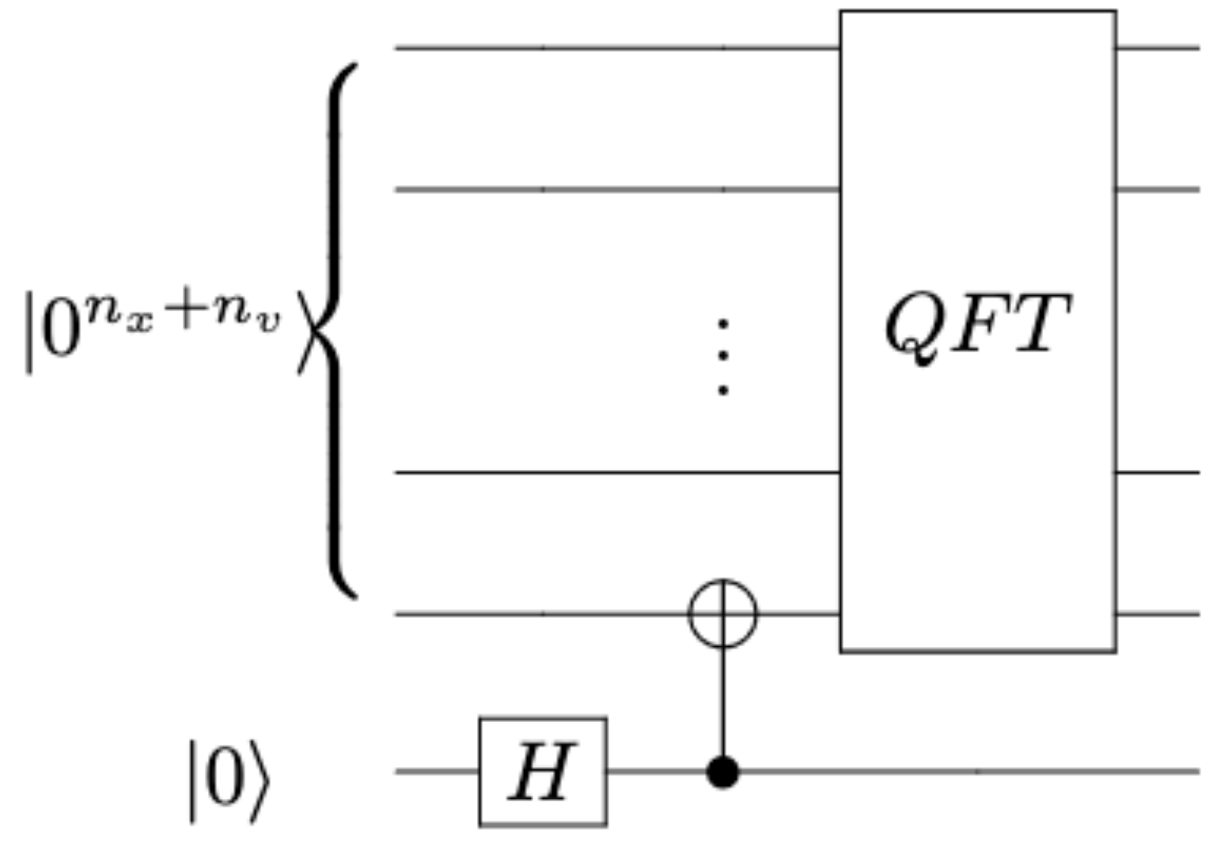
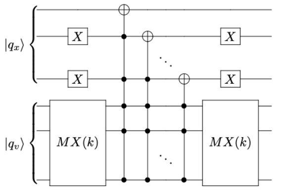
The key idea is to assign $f_{k;j}$ to quantum states by labeling or indexing. Let us consider a bijective mapping $\mathcal{M}:\mathbb{Z}/2^{n_{x}}\mathbb{Z}\times\mathbb{Z}/2^{n_{v}}\mathbb{Z}\rightarrow\mathbb{Z}/2^{n_{x}+n_{v}}\mathbb{Z}$ such that $\mathcal{M}((j,k))=2^{n_{v}}j+k$. We label each element in phase-space by $\mathcal{M}$, and embed the label, instead of the value of $f_{k;j}$, into the phase of a quantum state using quantum Fourier transform (QFT):

$$\mbox{QFT}\cdot\left(I^{n_{x}+n_{v}-1}\otimes CX_{a_{0},v_{n_{v}-1}}\right)\ket{0^{n_{x}+n_{v}+1}}$$

$$= \frac{1}{\sqrt{2}^{n_{x}+n_{v}+1}}\sum_{j=0}^{2^{n_{x}+n_{v}}-1}\ket{j}\otimes\left(\exp\left[\frac{2\pi ij}{2^{n_{x}+n_{v}}}\right]\ket{1}+\ket{0}\right)$$

. (11)

The corresponding quantum circuit is depicted in Fig. 1. The ancilla qubit is added to the quantum state in order to estimate the labels by the process of quantum state tomography (Sec. 3.3). The “proxy” of $f_{k;j}$ can be embedded into the quantum state in this manner. This is well suited to our reservoir method which preserves the values of $f_{k;j}$. The advection operation simply transfers $f_{k;j}$ in phase-space without changing the value itself, and thus it is sufficient to transfer the initial label of the discretized velocity distribution function. At the end of a simulation, one can retrieve the actual value of $f_{k;j}$ by the $\mathcal{M}^{-1}$ mapping.

Other methods for initialization are introduced in Appendix B, and the relevant elements of quantum gates are explained in Appendix A.

3.2 Updating $f_{k;j}$

From the definition of $v_{k}$, the time when $C_{k}=\pm 1$ can be calculated from $i/{|v_{k}|}$ for all $i=1,2,\dots$. We fix the time steps to

$$\begin{split}\{t_{i}\}_{i=0,1,2,\dots}&=\mbox{sorted sequence of}\\ &\left\{\frac{i}{|v_{k}|}\leavevmode\nobreak\ \middle|\leavevmode\nobreak\ i=0,1,2,\dots,\leavevmode\nobreak\ \leavevmode\nobreak\ k=0,1,\dots,2^{n_{v}}-1\right\}\end{split}$$ (12)

so that the simulation proceeds in this order by counting and resetting $D_{j}$ in the manner explained in the next section.

At each time step, we first perform advection in velocity space, followed by advection in the configuration space.

3.2.1 Advection in velocity space

We first update the CFL counter $D_{j}$ as

$$D_{j}\leftarrow D_{j}+F_{j}\frac{\Delta t_{n}}{\Delta v}.$$ (13)

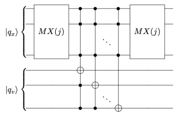
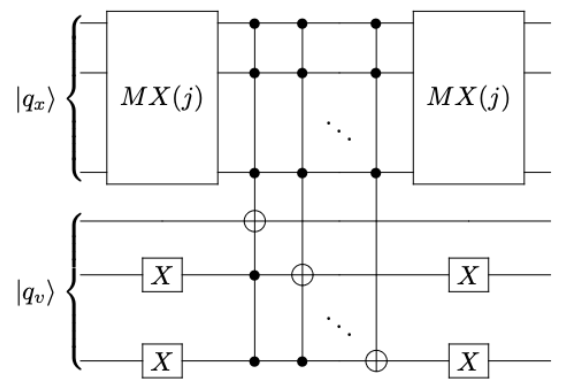
If $D_{j}>0$, we use a quantum circuit in Fig. 2 for $\lfloor D_{j}\rfloor$ times, and then we reset $D_{j}$ as

$$D_{j}\leftarrow D_{j}-\lfloor D_{j}\rfloor.$$ (14)

Otherwise, we use a quantum circuit in Fig. 2 for $\lceil D_{j}\rceil$ times, and reset $D_{j}$ as

$$D_{j}\leftarrow D_{j}-\lceil D_{j}\rceil.$$ (15)

Here, $\lfloor\cdot\rfloor$ is a floor function that returns the largest integer less than or equal to the input number, and $\lceil\cdot\rceil$ is a ceiling function that returns the smallest integer more than or equal to the input number.

The circuit of Fig. 2 effectively performs an increment to the index of the velocity coordinate at the position of spacial coordinate index $j$. This operation corresponds to advection in velocity space over precisely one grid.

3.2.2 Advection in configuration space

We perform the advection operation only for grids with the velocity index $k$ such that $t_{i}v_{k}\in\mathbb{Z}$. If $v_{k}>0$, a quantum circuit in Fig. 3 is used, and otherwise the one in Fig. 3 is used. The above sequence of operations complete the quantum version of the reservoir method in phase space.

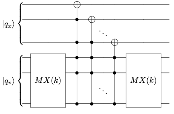
3.3 Information extraction

After the advection operations, the resulting “solution” would be the quantum state of the following form

$$\frac{1}{\sqrt{2}^{n_{x}+n_{v}+1}}\sum_{j=0}^{2^{n_{x}+n_{v}}-1}\ket{j}\otimes\left(\exp\left[\frac{2\pi i\sigma(j)}{2^{n_{x}+n_{v}}}\right]\ket{1}+\ket{0}\right),$$ (16)

where $\sigma$ is an element of a symmetry group, $\sigma\in\mathfrak{S}_{2^{n_{x}+n_{v}}}$. We can extract the labels $\sigma$ by a combination of quantum state tomography [5] and eigendecomposition. Eigendecomposition is used to get the resulting quantum state $\ket{\Psi}$ from a density matrix $\rho$ obtained from the quantum state tomography:

$$\rho=\ket{\Psi}\bra{\Psi}.$$ (17)

Then we obtain the value of $f_{k;j}$ by associating the labels with $f_{\mathcal{M}^{-1}(\sigma)}$.

3.4 Systems with variable forces

For general self-gravitating systems, we need to calculate the gravitational force field $F$ at every time step. If on a classical computer, a straightforward way would be to solve Poisson equation

$$\nabla^{2}\phi=4\pi G\rho(x)$$ (18)

from the density field

$$\rho(x)=\int f(x,v)\,{\rm d}v,$$ (19)

and then calculate the force as the spacial derivative of potential $\phi$. On a quantum computer, integration or even simple summation is a non-trivial task. We do not implement a quantum Poisson solver in our simulations in the present paper, but propose an efficient way to compute the mass density $\rho$ as a sum of the velocity distribution function. In Appendix B, we describe a particular method to compute the sum of $f_{k;j}$ by operating H gates. Once the density field as a sum of $f_{k;j}$ is calculated, the gravitational potential (and hence the force) field can be derived by solving Poisson equation. There are several promising quantum Poisson solvers proposed recently [6, 7, 8, 9, 10]. Combining with such an efficient quantum solver will enable a fully consistent quantum simulation, and we will enjoy advantages such as single measurement error and very low computational complexity.

In practice, for the simulations we present in the next section, we solve Poisson equation classically as in Ref. [1] and use the values of $F$ in the quantum advection operation in velocity space.

4 Computational complexity

We first discuss the time complexity of our numerical algorithm. A system’s characteristic time is $T=1/\mbox{min}(|v_{k}|)$. This is a basis for the analysis of time complexity. The Toffoli gates are assumed to be executed with the complexity of $\mathcal{O}(1)$ in this section, and also $N_{v}$ in Eq. (27) is assumed for the simulation to work. Advection in velocity space is executed $\mathcal{O}(L^{d}F_{s}T/\Delta v)=\mathcal{O}(L^{d}N_{v})$ times every system time $T$, where $d$ denotes the spatial dimension we consider, $L$ denotes the size of the computational domain, and $F_{s}$ is a characteristic magnitude of $F$. Advection in configuration space takes place $\mathcal{O}(dN_{v}^{2})$ times every system time $T$. Because the number of $X$ and Toffoli gates in the quantum circuit for both advection is $\mathcal{O}(n_{x}+n_{v})$, it costs $\mathcal{O}((n_{x}+n_{v})N_{v}(L^{d}+dN_{v}))$ per system time $T$ considering all of the above while classical reservoir method costs $\mathcal{O}(dN_{v}^{d+1}L^{d})$ [2].

We assume here that we perform the advection calculations using a quantum computer whereas the gravity calculation is done by using a classical computer (Sec. 3.4). Namely, we take a hybrid approach. The overall accuracy of the solution will not be affected significantly if we calculate $F$ every advection or every $1/\max(|v_{k}|)$, and thus we assume that the calculation of $F$ is done every $1/\max(|v_{k}|)$. It costs $\mathcal{O}(L^{d}\log L)$ for calculation of $F$, which does not change the time complexity. Note the significant decrease in dimension of $O(N_{v}^{3})$ compared to the classical calculation in three dimension. If measurement is to be performed every time step in order to get data of $f_{k;j}$ at an intermediate step, it would then be necessary to reproduce the state as the initial condition for continuation, which can add to the time complexity. In the future, this increase in time complexity can be avoided if quantum computers capable of parallel computing are available.

The number of required qubits without ancilla qubits is $n_{x}+n_{v}$, and that of ancilla qubits is $\mathcal{O}(n_{x}+n_{v})$. In a classical computer, however, we need to hold $\mathcal{O}(L^{3})$ CFL counters $D_{j}$. Therefore, space complexity amounts a total of $\mathcal{O}(L^{3}+n_{v})$.

5 Numerical Simulations

We have implemented the algorithm described so far using qiskit version 0.23.6 and QASM Simulator backend in aer, which are open-source software development kit with quantum computers and its simulator. We have performed the following test calculations [1] using Python version 3.8.6 because simulations on currently available quantum computers are still expensive.

5.1 Free Streaming

Figure 4: Snapshots of the one-dimensional free-streaming simulation with $F=0$ and $n_{x}=n_{v}=6$. From left to right, the distribution function $f$ at $t=0,1,2$, and $3$ cycles are shown. A white "box" at $t=0$ flows without deformation other than shearing in phase space.

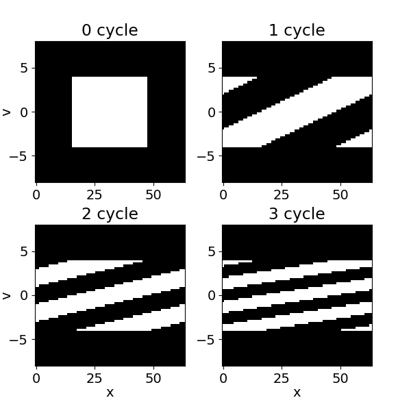
We set $F=0$, $n_{x}=n_{v}=6$, and configure a “box” initial condition for $f$ as shown in Fig. 4, where the white region has $f=1$ and black region $f=0$. The exact solution should be simple free streaming in phase space, and $f$ is advected over time to produce shear motion. The reservoir method does not allow deformation other than shearing, which we confirm with our numerical result.

5.2 Jeans instability

Figure 5: One-dimensional Jeans collapse with $n_{x}=n_{v}=6$ and with $A=0.1$, $k=0.5k_{\text{J}}$. The values of $f$ at $t=0,1,2,$ and $3$ are shown (see the colorbar on the right).

Figure 6: The time evolution of the Fourier amplitude $A_{2}$ of the density fluctuations in the run with $k/k_{\text{J}}=0.5$. We compare with the linear growth rate.

Our next example is one-dimensional gravitational instability. The force field $F$ is the fluid’s self-gravity. For a homogeneous mass distribution, there exists a stationary solution, i.e., the Maxwell distribution

$$f_{\mathrm{M}}(x,v)=\frac{\rho_{\mathrm{ref}}}{\sqrt{2\pi\sigma^{2}}}\exp\left(-\frac{v^{2}}{2\sigma^{2}}\right).$$ (20)

We add a perturbation of

$$f(x,v)=f_{\mathrm{M}}(x,v)(1+A\cos kx)$$ (21)

with $A=0.1,k=0.5k_{\text{J}}$ where the Jeans wavenumber is given by

$$k_{\mathrm{J}}=\frac{\sqrt{4\pi G\rho_{\mathrm{ref}}}}{\sigma}.$$ (22)

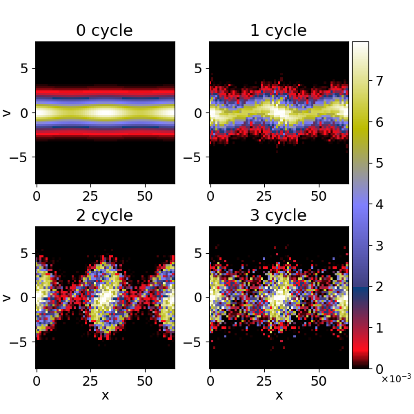
Fig. 5 shows the outputs of our simulation. The phase-space structure is followed accurately up to $t=2$ with the relatively low resolution with $n_{x}=n_{v}=6$, compared to the result of the high-accuracy classical simulation of Ref. [1] (see their Figure 6 on $128\times 128$ grids). At $t=3$, the distribution appears noisy, and the spiral structure commonly seen in high-resolution simulations is not well reproduced. This is likely owing to the coarse resolution of our simulation.

(a) $n_{v}=6$

(b) $n_{v}=11$

Figure 7: Comparison with an analytical solution of Fourier transform $A_{2}$ of the density fluctuation with $k/k_{\text{J}}=1.5$. Left figure shows the result of $n_{v}=6$ and right one shows the result of $n_{v}=11$. Only $n_{v}=11$ allows us to simulate $A_{2}$ with the same growth rate as the analytical solution.

From the initial condition Eq. (21), we can calculate the analytical solution for linear growth part of Fourier transform $A_{m}$ of $\delta(x,t)=\rho(x,t)-\rho_{\mathrm{ref}}$ [11], which is defined as

$$\delta(x,t)=\sum_{m\geq 0}A_{m}(t)\exp(im\frac{2\pi}{2^{n_{x}}}x).$$ (23)

The linear growth rate $\gamma$ is obtained by solving the plasma dispersion relation

$$(k/k_{\text{J}})^{2}= 1+wZ(w),$$

$$w= \frac{\pm i\gamma}{\sqrt{8\pi G\rho}\,(k/k_{\text{J}})},$$

$$Z(w)= \frac{1}{\sqrt{\pi}}\int_{-\infty}^{\infty}{\rm d}s\frac{e^{-s^{2}}}{s-w}.$$ (24)

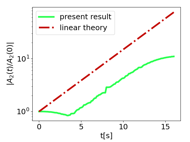
Fig. 6 shows that the growth of the perturbation is reproduced as predicted by linear theory. We thus conclude that our numerical scheme is well suited to follow the evolution of one-dimensional self-gravitating systems.

6 Discussion

We have developed a quantum algorithm based on the reservoir method to solve the collisionless Boltzmann equation on a quantum computer. We have successfully performed simulations of self-gravitating systems.

We discuss here the limitation of our numerical simulation. With the current implementation, the number of discrete grids in velocity space is $N_{v}=2^{n_{v}}$. The corresponding time step width $\Delta t_{c}$ necessary for update is, at each space point,

$$\Delta t_{c}=\frac{\Delta x}{\max(|v_{k}|)}=\frac{N_{v}\Delta x}{V(N_{v}-1)},$$ (25)

whereas the reservoir method requires

$$F_{s}\frac{\Delta t_{c}}{\Delta v}=\mathcal{O}(1),$$ (26)

where $F_{s}$ is a characteristic magnitude of $F$ and $\Delta v=2V/N_{v}$. If this condition is not met, the advection operation in velocity space does not take place for a sufficiently large number of times, leading to inaccurate evolution of the velocity distribution function. This effectively imposes a requirement on the velocity space resolution of

$$N_{v}=\mathcal{O}\left(\frac{V^{2}}{F_{s}\Delta x}\right).$$ (27)

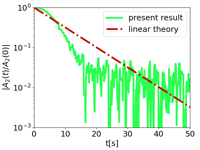
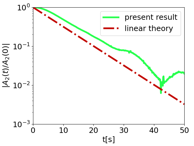
To examine the effect of insufficient resolution, we have performed simulations of gravitational Landau damping [11] with $k=1.5k_{\text{J}}$ for two setups with $n_{v}=6$ and $n_{v}=11$. The other conditions are kept the same as in Sec. 5.2. We plot the measured Fourier amplitude of $A_{2}$ and the damping rate in Fig. 7 and 7. Clearly, the run with poor resolution with $n_{v}=6$ yields too rapid damping and spurious oscillations, whereas the run with $n_{v}=11$ reproduces the correct initial damping as predicted by linear theory. We find that Eq. (27) serves as a practical condition to be checked and monitored through a simulation.

We have proposed a method that utilizes two separate CFL counters for advection in configuration space and in velocity space in an operator-splitting manner (Sec. 2). It allows us to perform simulations with a variable force field under the condition and limitation as discussed in the above. With the small computational complexity as derived in Sec. 4, future quantum computing has the potential to perform very large collisionless Boltzmann simulations. In our future work, we study applications to general Vlasov–Poisson systems including electro-static and electro-magnetic plasma.

Figure 8: Quantum circuit for embedding $f_{k;j}$ in the phase.

Appendix A Quantum gates

An $n$-qubits gate $MX(N)$, where $0\leq N\leq 2^{n}-1$, is defined by a set of $X$-gates as

$$MX(N)=\bigotimes_{i=0}^{n-1}X^{1-N_{i}},$$ (28)

where $N_{i}$ is the $(n-i)$-th digit of the binary expression of $N$.

A single qubit gate $R(n,i)$ is defined by $R_{y}$ as

$$R(n,i)=R_{y}(2\lambda(n,i)),$$ (29)

where

$$\lambda(n,i)=\arccos\left(\sqrt{\frac{\sum\limits_{j=0}^{2^{n_{x}+n_{v}-n-1}-1}f_{j+i*2^{n_{x}+n_{v}-n}}}{\sum\limits_{j=0}^{2^{n_{x}+n_{v}-n}-1}f_{j+i*2^{n_{x}+n_{v}-n}}}}\right)$$ (30)

with a convention that labels an index by the mapping ${\cal M}^{-1}$

$$f_{l}=f_{\left(l\leavevmode\nobreak\ \mathrm{mod}\leavevmode\nobreak\ 2^{n_{v}}\right);\lfloor l/2^{n_{v}}\rfloor}.$$ (31)

Figure 9: Quantum circuit for putting $f_{k;j}$ in the coefficient magnitude.

Appendix B Initialization and information extraction

We have proposed an initialization method in Sec. 3.1. Generating an arbitrary quantum state itself is a hard problem, but there are several possible manners to initialize a quantum state, and here we consider four different methods. The first one utilizes the phase of a quantum state. The value of $f_{k;j}$ can be embedded in the phase of a quantum state as

$$\frac{1}{\sqrt{2}^{n_{x}+n_{v}+1}}\sum_{j=0}^{2^{n_{x}}-1}\sum_{k=0}^{2^{n_{v}}-1}\ket{j}\otimes\ket{k}\otimes\left(\ket{0}+\exp\left[i\frac{f_{k;j}}{M_{p}}\pi\right]\ket{1}\right),$$ (32)

where $M_{p}$ is a real number greater than or equal to the maximum of $f_{k;j}$. This quantum state can be realized using the quantum circuit shown in Fig. 8. At the end of a numerical simulation, the values of $f_{k;j}$ in the form of Eq. (32) can be retrieved by a combination of quantum state tomography and eigendecomposition.

The second method assigns $f_{k;j}$ as coefficients of the quantum state as

$$\frac{1}{\sqrt{M_{1}}}\sum_{j=0}^{2^{n_{x}}-1}\sum_{k=0}^{2^{n_{v}}-1}\sqrt{f_{k;j}}\ket{j}\otimes\ket{k},$$ (33)

where $M_{1}$ is the sum of $f_{k;j}$ over all $k$ and $j$. Ref. [12] proposes an efficient algorithm to generate a realization of a designated probability distribution. The corresponding quantum state can be generated using the quantum circuit in Fig. 9. The final solution of a simulation can be obtained by considering the velocity distribution function as a probability $P_{k;j}$ on the grid $(x_{j},v_{k})$:

$$f_{k;j}=M_{1}P_{k;j}.$$ (34)

Obviously estimating the probability requires repeated measurements for a number of realizations.

As yet another approach, the values of $f_{k;j}$ can be assigned as the amplitudes of a quantum state as

$$\frac{1}{\sqrt{M_{2}}}\sum_{j=0}^{2^{n_{x}}-1}\sum_{k=0}^{2^{n_{v}}-1}f_{k;j}\ket{j}\otimes\ket{k},$$ (35)

where $M_{2}$ is a sum of $f_{k;j}^{2}$ over all $k$ and $j$. This quantum state can be realized using the quantum circuit similar to Fig. 9. We can retrieve the final distribution function $f_{k;j}=\sqrt{M_{2}P_{k;j}}$ as a probability distribution similarly to the description in the above.

The fourth method is to represent $f_{k;j}$ in an approximate manner by using ancilla qubits as

$$\frac{1}{\sqrt{2^{n_{x}+n_{v}}}}\sum_{j=0}^{2^{n_{x}}-1}\sum_{k=0}^{2^{n_{v}}-1}\ket{j}\otimes\ket{k}\otimes\ket{\tilde{f}_{k;j}},$$ (36)

where $\tilde{f}_{k;j}$ is the integer part of $f_{k;j}$ multiplied by a (large) constant. This quantum state can be easily realized by Toffoli gates. By repeating measurement, we can collect $\tilde{f}_{k;j}$. Dividing $\tilde{f}$ by the same constant, we finally get the values of $f_{k;j}$.

For collisionless Boltzmann simulations of self-gravitating systems, one needs to calculate the integral of the distribution function

$$\rho(x)=\int f(x,v)\,{\rm d}v.$$ (37)

The density field $\rho(x)$ is used to calculate the gravitational force field $F(x)$ via Poisson equation. To this end, an efficient method of calculating $\rho(x)$ is needed. We propose two ways to achieve this. If we adopt the representation of Eq. (33), we obtain

$$\rho_{j}=\Delta vM_{1}P_{j},$$ (38)

where $P_{j}=\sum_{k}P_{k,j}$ (Eq. [34]). Alternatively, if we adopt the representation of Eq. (35), we operate H gates to the quantum state $\ket{\psi}$ after the advection operation as

$$\left(I^{\otimes n_{x}}\otimes H^{\otimes n_{v}}\right)\ket{\psi}$$

$$=\frac{1}{\sqrt{M_{2}}}\sum_{j=0}^{2^{n_{x}}-1}\sum_{k=0}^{2^{n_{v}}-1}\sum_{l=0}^{2^{n_{v}}-1}f_{k;j}\frac{(-1)^{k\cdot l}}{\sqrt{2}^{n_{v}}}\ket{j}\otimes\ket{l}$$

$$=\frac{1}{\sqrt{2^{n_{v}}M_{2}}}\sum_{j=0}^{2^{n_{x}}-1}\sum_{l=0}^{2^{n_{v}}-1}\left(\sum_{k=0}^{2^{n_{v}}-1}(-1)^{k\cdot l}f_{k;j}\right)\ket{j}\otimes\ket{l},$$ (39)

where $\cdot$ denotes bitwise AND. This state holds $\rho_{j}$ for $l=0$. Note that the probability of the state $l=0$ being realized upon measurement is generally higher than other $l$s because $f_{k;j}\geq 0$ ; the coefficients tend to cancel each other unless $l=0$.

References

- [1] Kohji Yoshikawa, Naoki Yoshida, and Masayuki Umemura. “Direct Integration of the Collisionless Boltzmann Equation in Six-dimensional Phase Space: Self-gravitating Systems”. The Astrophysical Journal 762, 116 (2013).
- [2] Blaga N. Todorova and René Steijl. “Quantum algorithm for the collisionless Boltzmann equation”. Journal of Computational Physics 409, 109347 (2020).
- [3] F. Alouges, F. Devuyst, G. Lecoq, and E. Lorin. “The reservoir technique: a way to make Godunov-type schemes zero or very low diffuse. Application to Colella-Glaz solver”. European Journal of Mechanics B Fluids 27, 643–664 (2008).
- [4] F. Fillion-Gourdeau and E. Lorin. “Simple digital quantum algorithm for symmetric first-order linear hyperbolic systems”. Numerical Algorithms 82, 1009–1045 (2019).
- [5] Michael A. Nielsen and Isaac L. Chuang. “Quantum computation and quantum information: 10th anniversary edition”. Cambridge University Press. (2010).
- [6] Yudong Cao, Anargyros Papageorgiou, Iasonas Petras, Joseph Traub, and Sabre Kais. “Quantum algorithm and circuit design solving the Poisson equation”. New Journal of Physics 15, 013021 (2013). arXiv:1207.2485.
- [7] Shengbin Wang, Zhimin Wang, Wendong Li, Lixin Fan, Zhiqiang Wei, and Yongjian Gu. “Quantum fast Poisson solver: the algorithm and complete and modular circuit design”. Quantum Information Processing 19, 170 (2020).
- [8] Andrew M. Childs, Jin-Peng Liu, and Aaron Ostrander. “High-precision quantum algorithms for partial differential equations”. Quantum 5, 574 (2021).
- [9] Yuki Sato, Ruho Kondo, Satoshi Koide, Hideki Takamatsu, and Nobuyuki Imoto. “Variational quantum algorithm based on the minimum potential energy for solving the Poisson equation”. Physical Review A 104, 052409 (2021). arXiv:2106.09333.
- [10] Fong Yew Leong, Wei-Bin Ewe, and Dax Enshan Koh. “Variational quantum evolution equation solver”. Scientific Reports 12, 10817 (2022).
- [11] James Binney and Scott Tremaine. “Galactic dynamics: Second edition”. Princeton University Press. (2008). Rev - revised, 2 edition.
- [12] Lov Grover and Terry Rudolph. “Creating superpositions that correspond to efficiently integrable probability distributions” (2002). arXiv:quant-ph/0208112.