Spectral pseudorandomness and the road to improved clique number bounds for Paley graphs

Dmitriy Kunisky Email: dmitriy.kunisky@yale.edu. Partially supported by ONR Award N00014-20-1-2335 and a Simons Investigator Award to Daniel Spielman. Department of Computer Science, Yale University
(March 29, 2023)
Abstract

We study subgraphs of Paley graphs of prime order p𝑝p induced on the sets of vertices extending a given independent set of size a𝑎a to a larger independent set. Using a sufficient condition proved in the author’s recent companion work, we show that a family of character sum estimates would imply that, as p𝑝p\to\infty, the empirical spectral distributions of the adjacency matrices of any sequence of such subgraphs have the same weak limit (after rescaling) as those of subgraphs induced on a random set including each vertex independently with probability 2asuperscript2𝑎2^{-a}, namely, a Kesten-McKay law with parameter 2asuperscript2𝑎2^{a}. We prove the necessary estimates for a=1𝑎1a=1, obtaining in the process an alternate proof of a character sum equidistribution result of Xi (2022), and provide numerical evidence for this weak convergence for a2𝑎2a\geq 2. We also conjecture that the minimum eigenvalue of any such sequence converges (after rescaling) to the left edge of the corresponding Kesten-McKay law, and provide numerical evidence for this convergence. Finally, we show that, once a3𝑎3a\geq 3, this (conjectural) convergence of the minimum eigenvalue would imply bounds on the clique number of the Paley graph improving on the current state of the art due to Hanson and Petridis (2021), and that this convergence for all a1𝑎1a\geq 1 would imply that the clique number is o(p)𝑜𝑝o(\sqrt{p}).

1 Introduction

Let p1(mod 4)𝑝1mod4p\equiv 1\ (\mathrm{mod}\ 4) be prime. Let 𝔽psubscript𝔽𝑝\mathbb{F}_{p} be the finite field of order p𝑝p, identified with /(p)𝑝\mathbb{Z}/(p\mathbb{Z}) (the integers modulo p𝑝p), let 𝔽p×superscriptsubscript𝔽𝑝\mathbb{F}_{p}^{\times} be its multiplicative group (of non-zero elements), and let SSp<𝔽p×subscriptSS𝑝superscriptsubscript𝔽𝑝\SS_{p}<\mathbb{F}_{p}^{\times} be the subgroup of non-zero quadratic residues (those x0𝑥0x\neq 0 such that xy2(modp)𝑥superscript𝑦2mod𝑝x\equiv y^{2}\ (\mathrm{mod}\ p) for some y𝑦y). The Paley graph, defined on vertex set 𝔽psubscript𝔽𝑝\mathbb{F}_{p}, has xysimilar-to𝑥𝑦x\sim y if and only if xySSp𝑥𝑦subscriptSS𝑝x-y\in\SS_{p}.

The graphs Gpsubscript𝐺𝑝G_{p} are thought to be pseudorandom, behaving in many ways like Erdős-Rényi (ER) random graphs with edge probability 1212\frac{1}{2}, this probability chosen to match Gpsubscript𝐺𝑝G_{p} being (p12)𝑝12(\frac{p-1}{2})-regular. For example, the Gpsubscript𝐺𝑝G_{p} satisfy the “quasi-randomness” conditions described in [CGW89]; in particular, the extreme eigenvalues scale roughly similarly to those (typically) of an ER graph, and the number of appearances of any fixed graph G(0)superscript𝐺0G^{(0)} as an induced subgraph in Gpsubscript𝐺𝑝G_{p} as p𝑝p\to\infty scales as the number of appearances of G(0)superscript𝐺0G^{(0)} (typically) in an ER graph. Going on this intuition, the Gpsubscript𝐺𝑝G_{p} are believed to be useful for several derandomization problems. Namely, it is believed that deterministic matrices satisfying the restricted isometry property can be constructed from the closely related Paley equiangular tight frames [BFMW13, BMM17], and the Gpsubscript𝐺𝑝G_{p} themselves are believed to be explicit constructions of tight lower bounds on the diagonal Ramsey numbers. However, it seems difficult to prove such claims, as they require much more precise number-theoretic analysis than the above notions of pseudorandomness.

In this paper, we study new proof techniques for controlling the quantities involved in the latter Ramsey theory application.111See Appendix C for discussion of limitations of our approach for studying the restricted isometry property. For a graph G𝐺G, we write ω(G)𝜔𝐺\omega(G) for its clique number, G¯¯𝐺\overline{G} for its complement, and α(G)\colonequalsω(G¯)𝛼𝐺\colonequals𝜔¯𝐺\alpha(G)\colonequals\omega(\overline{G}) for its independence number. For the purposes of Ramsey theory, we are interested in showing that ω(Gp)𝜔subscript𝐺𝑝\omega(G_{p}) and α(Gp)𝛼subscript𝐺𝑝\alpha(G_{p}) are both small (see Section 1.7 for more discussion). For the Paley graph, Gpsubscript𝐺𝑝G_{p} is isomorphic to Gp¯¯subscript𝐺𝑝\overline{G_{p}}, so α(Gp)=ω(Gp)𝛼subscript𝐺𝑝𝜔subscript𝐺𝑝\alpha(G_{p})=\omega(G_{p}) and there is only one number to control. The literature usually discusses the clique number of the Paley graph, but here we will discuss the independence number instead, both for mild notational convenience later and to draw an analogy with similar problems below.

Consequences for Ramsey theory aside, determining α(Gp)𝛼subscript𝐺𝑝\alpha(G_{p}) is a prominent problem in number theory; for example, α(Gp)𝛼subscript𝐺𝑝\alpha(G_{p}) is an upper bound on the smallest quadratic non-residue modulo p𝑝p, determining which is another long-standing open problem. Through this connection, [GR90] showed that, for infinitely many primes p𝑝p,

α(Gp)logplogloglogp.𝛼subscript𝐺𝑝𝑝𝑝\alpha(G_{p})\geq\log p\log\log\log p. (1)

This is slightly larger than the typical value for an ER graph on p𝑝p vertices, which is of order Θ(logp)Θ𝑝\Theta(\log p). Conditional on the Generalized Riemann Hypothesis, the logloglogp𝑝\log\log\log p term can also be improved to loglogp𝑝\log\log p [Mon71, Theorem 13.5], and this is compatible with a more detailed random model of Gpsubscript𝐺𝑝G_{p} [Mra17]. More generally, based on such results as well as numerical computations of α(Gp)𝛼subscript𝐺𝑝\alpha(G_{p}), the following conjecture is widely believed.

Conjecture 1.1 ([She86, BMR13, Yip22, KY22]).

α(Gp)=O(𝗉𝗈𝗅𝗒𝗅𝗈𝗀(p))𝛼subscript𝐺𝑝𝑂𝗉𝗈𝗅𝗒𝗅𝗈𝗀𝑝\alpha(G_{p})=O(\mathsf{polylog}(p)).

As we detail in Section 1.7, proving this would yield a substantial improvement on the best known explicit construction of Ramsey graphs (ones giving strong lower bounds on the diagonal Ramsey numbers).

In stark contrast to Conjecture 1.1, the best known upper bound on α(Gp)𝛼subscript𝐺𝑝\alpha(G_{p}), due to Hanson and Petridis, is as follows.

Theorem 1.2 ([HP21, DBSW21]).

α(Gp)2p1+1212p+1𝛼subscript𝐺𝑝2𝑝11212𝑝1\alpha(G_{p})\leq\frac{\sqrt{2p-1}+1}{2}\leq\frac{1}{\sqrt{2}}\sqrt{p}+1.

This is only a modest improvement on the “trivial” bound α(Gp)p𝛼subscript𝐺𝑝𝑝\alpha(G_{p})\leq\sqrt{p}, which has many proofs: p𝑝\sqrt{p} is the value of both the spectral “Hoffman bound” and the Lovász ϑitalic-ϑ\vartheta function bounds on α(Gp)𝛼subscript𝐺𝑝\alpha(G_{p}) [Lov79, Theorem 8], and one may also obtain the same bound combinatorially [Yip22, Lemma 1.2].

1.1 Relaxation and localization: two bounding strategies

Beyond our lack of tight quantitative bounds on α(Gp)𝛼subscript𝐺𝑝\alpha(G_{p}), this state of affairs is conceptually disappointing because the known proofs of Theorem 1.2 use in a deep way the algebraic structure of Gpsubscript𝐺𝑝G_{p}. It would be more satisfying to treat α(Gp)𝛼subscript𝐺𝑝\alpha(G_{p}) in the same framework as other “packing” or independence number problems arising in extremal combinatorics and coding theory. In particular, convex relaxation bounds on α(Gp)𝛼subscript𝐺𝑝\alpha(G_{p})—bounds by linear (LP) or semidefinite (SDP) programs—have been useful for bounding independence numbers of many other graphs of interest [Del72, Lov79, CE03, Sch05, BV08, dLV15]. Can techniques based on convex relaxation improve on the state-of-the-art bound on α(Gp)𝛼subscript𝐺𝑝\alpha(G_{p})?

It is unclear whether to expect this approach to succeed. On the one hand, a long line of work has shown that, for ER random graphs G𝐺G, increasingly sophisticated convex relaxations of α(G)𝛼𝐺\alpha(G) do not improve substantially on simple spectral bounds (which may be viewed as very simple instances of convex relaxation). Perhaps most prominent among these results are those showing such lower bounds for the otherwise quite powerful sum-of-squares (SOS) hierarchy of semidefinite programs [MW13, MPW15, RS15, DM15, HKP+18, BHK+19, Pan21]. Thus, if we believe in sufficiently strong pseudorandomness of the Paley graph, we should not expect convex relaxations of α(Gp)𝛼subscript𝐺𝑝\alpha(G_{p}) to improve much on the p𝑝\sqrt{p} bound. On the other hand, the work of [GLV09] and the author’s recent results with Yu [KY22] suggest that such convex relaxations (in particular, the degree 4 SOS relaxation) might after all improve on the bound of Theorem 1.2 and even prove that α(Gp)=O(p12ε)𝛼subscript𝐺𝑝𝑂superscript𝑝12𝜀\alpha(G_{p})=O(p^{\frac{1}{2}-\varepsilon}) for some ε>0𝜀0\varepsilon>0. A possible reason for this is that the spectrum of Gpsubscript𝐺𝑝G_{p} is sufficiently different from that of an ER random graph: the eigenvalues of an ER graph have the semicircle distribution of random matrix theory, while Gpsubscript𝐺𝑝G_{p} is strongly regular and has only three distinct eigenvalues, a very differently-shaped empirical spectral distribution.222See the discussion of graph matrix norm bounds in [KY22] for how to convert this discrepancy into evidence that higher degrees of SOS may give improved bounds on α(Gp)𝛼subscript𝐺𝑝\alpha(G_{p}).

The recent work of [MMP19] contributed a complementary idea for bounding α(Gp)𝛼subscript𝐺𝑝\alpha(G_{p}), which we call the localization approach.333The localization approach is somewhat similar to the tools developed by Elias-Bassalygo and Kalai-Linial for bounding the independence numbers of interest in coding theory [Bas65, Ber68, KL95]. Let a(G)subscript𝑎𝐺\mathcal{I}_{a}(G) denote the set of independent sets of size a𝑎a in a graph G𝐺G. The idea is to bound α(G)𝛼𝐺\alpha(G) by enumerating all Ia(G)𝐼subscript𝑎𝐺I\in\mathcal{I}_{a}(G), and then to consider the independence number of graphs induced on all vertices extending I𝐼I to a larger independent set. The basic tool is the following.

Definition 1.3 (Localization).

For XV(Gp)𝑋𝑉subscript𝐺𝑝X\subseteq V(G_{p}), let Gp,Xsubscript𝐺𝑝𝑋G_{p,X} denote the subgraph of Gpsubscript𝐺𝑝G_{p} induced on the vertices not adjacent to any vertex of X𝑋X (not including vertices in X𝑋X itself). We call Gp,Xsubscript𝐺𝑝𝑋G_{p,X} a localization of G𝐺G of degree |X|𝑋|X|.

Proposition 1.4 (Localization bound).

For any aα(Gp)𝑎𝛼subscript𝐺𝑝a\leq\alpha(G_{p}),

α(Gp)=a+maxIa(Gp)ω(Gp,I).𝛼subscript𝐺𝑝𝑎subscript𝐼subscript𝑎subscript𝐺𝑝𝜔subscript𝐺𝑝𝐼\alpha(G_{p})=a+\max_{I\in\mathcal{I}_{a}(G_{p})}\omega(G_{p,I}). (2)

If one has some general upper bound α(G)f(G)𝛼𝐺𝑓𝐺\alpha(G)\leq f(G) for all graphs G𝐺G, then instead of bounding α(Gp)f(Gp)𝛼subscript𝐺𝑝𝑓subscript𝐺𝑝\alpha(G_{p})\leq f(G_{p}), one may bound by substituting f𝑓f into the right-hand side of (2):

α(Gp)a+maxIa(Gp)f(Gp,I).𝛼subscript𝐺𝑝𝑎subscript𝐼subscript𝑎subscript𝐺𝑝𝑓subscript𝐺𝑝𝐼\alpha(G_{p})\leq a+\max_{I\in\mathcal{I}_{a}(G_{p})}f(G_{p,I}). (3)

For example, [MMP19] took f(G)𝑓𝐺f(G) to be the Lovász function ϑ(G)italic-ϑ𝐺\vartheta(G), an SDP relaxation of α(G)𝛼𝐺\alpha(G) equivalent to the degree 2 SOS relaxation, with a=1𝑎1a=1. It turns out that the graphs Gp,{x}subscript𝐺𝑝𝑥G_{p,\{x\}} are isomorphic for all x𝔽p𝑥subscript𝔽𝑝x\in\mathbb{F}_{p} (see Corollary 3.2), so the method of [MMP19] only requires looking at one graph:

α(Gp)1+ϑ(Gp,{0}).𝛼subscript𝐺𝑝1italic-ϑsubscript𝐺𝑝0\alpha(G_{p})\leq 1+\vartheta(G_{p,\{0\}}). (4)

The graph Gp,{0}subscript𝐺𝑝0G_{p,\{0\}} is still highly symmetric, in particular having a circulant adjacency matrix, so ϑ(Gp,{0})italic-ϑsubscript𝐺𝑝0\vartheta(G_{p,\{0\}}) may be reduced to an LP and solved efficiently for large p𝑝p. Doing this, [MMP19] found empirically that the bound (4) usually almost exactly matches that of Theorem 1.2. Localization therefore improves the quality of the bound we obtain, from the trivial bound to one matching the state of the art:

α(Gp)𝛼subscript𝐺𝑝\displaystyle\alpha(G_{p}) ϑ(Gp)=pwithout localization,absentitalic-ϑsubscript𝐺𝑝𝑝without localization,\displaystyle\leq\vartheta(G_{p})=\sqrt{p}\,\,\,\text{without localization,} (5)
α(Gp)𝛼subscript𝐺𝑝\displaystyle\alpha(G_{p}) 1+ϑ(Gp,{0})12pwith degree 1 localization (empirically).absent1italic-ϑsubscript𝐺𝑝012𝑝with degree 1 localization (empirically).\displaystyle\leq 1+\vartheta(G_{p,\{0\}})\approx\frac{1}{\sqrt{2}}\sqrt{p}\,\,\,\text{with degree 1 localization (empirically).} (6)

Combining convex relaxation and localization, we have a family of strategies for bounding α(Gp)𝛼subscript𝐺𝑝\alpha(G_{p}) with two degrees of freedom: we may choose a degree of localization a𝑎a, choose a convex relaxation bound f𝑓f, and try to analyze the right-hand side of (3). For fixed a𝑎a, strengthening the bound f𝑓f will improve the result. Extrapolating from the results of [MMP19], it seems reasonable to expect that, for fixed f𝑓f, increasing the degree of localization a𝑎a will also improve the result. But how specifically do these two choices interact? To understand this, we must understand the localizations Gp,Isubscript𝐺𝑝𝐼G_{p,I} in greater detail.

1.2 Random model for Paley graph localizations

The main thesis of this paper is that the localizations Gp,Isubscript𝐺𝑝𝐼G_{p,I} have a collection of properties we call spectral pseudorandomness. The idea is that the spectrum of Gp,Isubscript𝐺𝑝𝐼G_{p,I} behaves like that of an induced subgraph on a random subset of vertices of Gpsubscript𝐺𝑝G_{p} of comparable size. Note that the spectrum of Gpsubscript𝐺𝑝G_{p} itself, as noted above, is not close to that of an ER graph of the same size. In introducing the notion of spectral pseudorandomness, we are proposing a more fine-grained way in which pseudorandomness does appear in the spectral structure of Gpsubscript𝐺𝑝G_{p}.

Definition 1.5 (Random Paley subgraphs).

Let Hp,βsubscript𝐻𝑝𝛽H_{p,\beta} be the random graph formed as follows: form a subset W𝔽p𝑊subscript𝔽𝑝W\subseteq\mathbb{F}_{p} randomly by including every vertex independently with probability β𝛽\beta, and let Hp,βsubscript𝐻𝑝𝛽H_{p,\beta} be the subgraph induced by Gpsubscript𝐺𝑝G_{p} on W𝑊W.

We then propose that Gp,Isubscript𝐺𝑝𝐼G_{p,I} behaves like Hp,βsubscript𝐻𝑝𝛽H_{p,\beta} with β=2|I|𝛽superscript2𝐼\beta=2^{-|I|}. The intuition behind the choice of β𝛽\beta is that xV(Gp,I)𝑥𝑉subscript𝐺𝑝𝐼x\in V(G_{p,I}) if x𝑥x is not adjacent to each yI𝑦𝐼y\in I. If Gpsubscript𝐺𝑝G_{p} is pseudorandom, these non-adjacencies may be viewed as |I|𝐼|I| “independent” events that each occur with “probability” 1212\frac{1}{2}, for a total “probability” of 2|I|superscript2𝐼2^{-|I|} that any given xV(Gp,I)𝑥𝑉subscript𝐺𝑝𝐼x\in V(G_{p,I}).

The empirical spectral distribution (e.s.d.) of a matrix 𝑨symn×n𝑨subscriptsuperscript𝑛𝑛sym\bm{A}\in\mathbb{R}^{n\times n}_{\operatorname{sym}} is the probability measure 1ni=1nδλi(𝑨)1𝑛superscriptsubscript𝑖1𝑛subscript𝛿subscript𝜆𝑖𝑨\frac{1}{n}\sum_{i=1}^{n}\delta_{\lambda_{i}(\bm{A})}. The e.s.d. of a graph is the e.s.d. of its adjacency matrix. In this language, we claim that, for large p𝑝p and small |I|𝐼|I|, the (deterministic) e.s.d. of Gp,Isubscript𝐺𝑝𝐼G_{p,I} is close to the typical (random) e.s.d. of Hp,2|I|subscript𝐻𝑝superscript2𝐼H_{p,2^{-|I|}}. Below we will give a collection of conjectures describing this closeness in different quantitative senses. Strong enough such statements, controlling the minimum eigenvalue of Gp,Isubscript𝐺𝑝𝐼G_{p,I}, will let us apply the localization strategy effectively with f(G)𝑓𝐺f(G) a spectral bound on α(G)𝛼𝐺\alpha(G).

The following recent result, first proposed as part of a collection of conjectures by [HZG17], describes the limiting e.s.d. of the Hp,2|I|subscript𝐻𝑝superscript2𝐼H_{p,2^{-|I|}}. We will argue that the e.s.d.’s of the Gp,Isubscript𝐺𝑝𝐼G_{p,I} are close to these measures.

Definition 1.6 (Kesten-McKay measure).

For v1𝑣1v\geq 1, the Kesten-McKay measure with parameter v𝑣v, denoted 𝖪𝖬(v)𝖪𝖬𝑣\mathsf{KM}(v), is the probability measure on \mathbb{R} with density

1{|x|2v1}v4(v1)x22π(v2x2)dx+max{2v,0}2δv(x)+max{2v,0}2δv(x),1𝑥2𝑣1𝑣4𝑣1superscript𝑥22𝜋superscript𝑣2superscript𝑥2𝑑𝑥2𝑣02subscript𝛿𝑣𝑥2𝑣02subscript𝛿𝑣𝑥\mathbbold{1}\{|x|\leq 2\sqrt{v-1}\}\frac{v\sqrt{4(v-1)-x^{2}}}{2\pi(v^{2}-x^{2})}\,dx+\frac{\max\{2-v,0\}}{2}\delta_{-v}(x)+\frac{\max\{2-v,0\}}{2}\delta_{v}(x), (7)

where δcsubscript𝛿𝑐\delta_{c} denotes a Dirac mass at c𝑐c.

Let us write 𝑨Gsubscript𝑨𝐺\bm{A}_{G} for the adjacency matrix of a graph G𝐺G.

Theorem 1.7 ([MMP21, Kun23]).

The (random) e.s.d. of 2βp𝐀Hp,β2𝛽𝑝subscript𝐀subscript𝐻𝑝𝛽\frac{2}{\beta\sqrt{p}}\bm{A}_{H_{p,\beta}} converges weakly in probability444Random measures μnsubscript𝜇𝑛\mu_{n} converge weakly in probability to a deterministic measure μ𝜇\mu if μn(A)μ(A)subscript𝜇𝑛𝐴𝜇𝐴\mu_{n}(A)\to\mu(A) in probability for every measurable set A𝐴A. to 𝖪𝖬(1/β)𝖪𝖬1𝛽\mathsf{KM}(1/\beta) as p𝑝p\to\infty.

A direct combinatorial proof of a minor variation on this was first given by [MMP21], while [Kun23] later observed that this result is a consequence of a more general asymptotic freeness (in the sense of free probability) phenomenon. We will eventually exploit this connection in our arguments; see the discussion around Conjecture 4.1.

1.3 A relaxation-localization tradeoff?

Before proceeding to our specific conjectures and results, let us comment generally on what spectral pseudorandomness might imply for our earlier question of how relaxation and localization interact.

As v𝑣v\to\infty, the measures 𝖪𝖬(v)𝖪𝖬𝑣\mathsf{KM}(v) converge, after rescaling, to the semicircle law (see Figure 1 for an illustration). Thus, a consequence of spectral pseudorandomness is that, as the degree of localization increases, the localizations of Gpsubscript𝐺𝑝G_{p} more and more resemble (at the level of the spectrum) ER random graphs.

But, as mentioned earlier, on ER random graphs, stronger convex relaxations of α(G)𝛼𝐺\alpha(G) are essentially no more effective than weaker relaxations or a basic spectral bound. It is perhaps reasonable to extrapolate this to the claim that, the more G𝐺G resembles an ER random graph at the level of the spectrum, the less “return on investment” we get from bounding α(G)f(G)𝛼𝐺𝑓𝐺\alpha(G)\leq f(G) with a more computationally expensive convex relaxation f(G)𝑓𝐺f(G).

We thus arrive at the following intuitive idea: increasing the convex relaxation strength is more helpful at low degrees of localization and less helpful at higher degrees of localization; increasing the degree of localization is more helpful for weak convex relaxations and less helpful for strong convex relaxations. If this is true, we should be able to “trade” higher degrees of localization for weaker convex relaxations while obtaining comparable bounds. This would be convenient because, for proving actual results, it seems hard to analyze sophisticated convex relaxations applied to deterministic pseudorandom graphs (as attempted for SOS relaxations on Paley graphs by [MMP19, KY22]).

In Table 1, we present the combinations of relaxation and localization that have been examined before for Paley graphs and those that we look at in this paper. To summarize, prior work has examined a few SOS relaxations with low degrees of localization, while we mostly restrict our attention to the weaker spectral bound but consider arbitrary degrees of localization. We focus on this case because the spectrum of Gp,Isubscript𝐺𝑝𝐼G_{p,I}, characterized by spectral pseudorandomness, already gives enough information to compute the spectral bound. And we will show that, conditional on natural conjectures, even spectral bounds can prove strong bounds on α(Gp)𝛼subscript𝐺𝑝\alpha(G_{p}) provided we combine them with high degrees of localization. We leave the task of filling in the missing entries in Table 1—characterizing how more sophisticated convex relaxations interact with localization—to future work.

Localization degree a𝑎a
0 1 2 3absent3\geq 3
Bound f(G)𝑓𝐺f(G) Spectral folklore (p)p{}^{(\text{p})} this paper (p)p{}^{(\text{p})} this paper (c)c{}^{(\text{c})} this paper (c)c{}^{(\text{c})}
SOS degree 2 implicitly [Lov79](p)p{}^{(\text{p})} [MMP19](e)e{}^{(\text{e})} this paper (e)e{}^{(\text{e})} ?
SOS degree 4 [KY22](p,e)pe{}^{(\text{p},\text{e})} ? ? ?
SOS degree 6absent6\geq 6 ? ? ? ?
Table 1: Known relaxation-localization bounds. We summarize the analyses of combinations of localization and convex relaxation that have been performed for bounding α(Gp)=ω(Gp)𝛼subscript𝐺𝑝𝜔subscript𝐺𝑝\alpha(G_{p})=\omega(G_{p}) in the literature. We mark those works that prove results on these bounds by (p)p(\text{p}), those works that prove results conditional on conjectures by (c)c(\text{c}), and those works that give empirical or numerical evidence by (e)e(\text{e}). We note that degree 2 SOS is equivalent to the Lovász ϑitalic-ϑ\vartheta function, and that we examine degree 2 localization combined with this relaxation in Appendix A.

1.4 Spectral pseudorandomness conjectures

We now present our specific conjectures about spectral pseudorandomness. We will phrase all of our conjectures in terms of the degree a1𝑎1a\geq 1 of the localizations involved.

Our first conjecture states our claim of spectral pseudorandomness at the level of weak convergence.

Conjecture 1.8 (Weak convergence, degree a𝑎a).

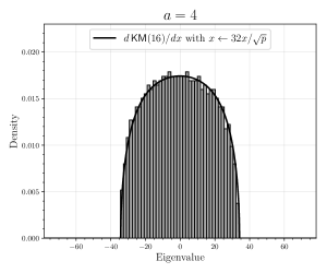
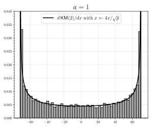
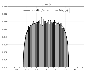
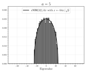
For all p𝑝p sufficiently large, let Ia(Gp)𝐼subscript𝑎subscript𝐺𝑝I\in\mathcal{I}_{a}(G_{p}). Then, the (deterministic) e.s.d. of 2a+1p𝐀Gp,Isuperscript2𝑎1𝑝subscript𝐀subscript𝐺𝑝𝐼\frac{2^{a+1}}{\sqrt{p}}\bm{A}_{G_{p,I}} converges weakly to 𝖪𝖬(2a)𝖪𝖬superscript2𝑎\mathsf{KM}(2^{a}).

This will follow from the more technical but more powerful Conjecture 4.1, which states that a pair of projection matrices associated to Gpsubscript𝐺𝑝G_{p} and to I𝐼I, respectively, are asymptotically free. This allows us to treat Conjecture 1.8 with the tools developed by [Kun23]. See Section 1.7 for some discussion of the interest of Conjecture 4.1 for free probability theory.

Our second conjecture gives a form of spectral pseudorandomness “at the edge,” concerning the minimum eigenvalue of the adjacency matrix.555It would also be reasonable to make the same conjecture for the maximum eigenvalue, though one should exclude the large isolated Perron-Frobenius eigenvalue.

Conjecture 1.9 (Minimum eigenvalue, degree a𝑎a).

We have

limpminIa(Gp)2a+1pλmin(𝑨Gp,I)=limpmaxIa(Gp)2a+1pλmin(𝑨Gp,I)=22a1.subscript𝑝subscript𝐼subscript𝑎subscript𝐺𝑝superscript2𝑎1𝑝subscript𝜆subscript𝑨subscript𝐺𝑝𝐼subscript𝑝subscript𝐼subscript𝑎subscript𝐺𝑝superscript2𝑎1𝑝subscript𝜆subscript𝑨subscript𝐺𝑝𝐼2superscript2𝑎1\lim_{p\to\infty}\min_{I\in\mathcal{I}_{a}(G_{p})}\frac{2^{a+1}}{\sqrt{p}}\lambda_{\min}(\bm{A}_{G_{p,I}})=\lim_{p\to\infty}\max_{I\in\mathcal{I}_{a}(G_{p})}\frac{2^{a+1}}{\sqrt{p}}\lambda_{\min}(\bm{A}_{G_{p,I}})=-2\sqrt{2^{a}-1}. (8)

Note that the left-hand side has the same normalization as in Conjecture 1.8, while the right-hand side is the left edge of the support of 𝖪𝖬(2a)𝖪𝖬superscript2𝑎\mathsf{KM}(2^{a}).

Remark 1.10 (Symmetry in low-degree localizations).

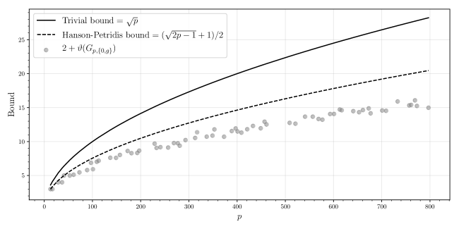
The cases a{1,2}𝑎12a\in\{1,2\} of these statements are especially simple, because for either of these values the Gp,Isubscript𝐺𝑝𝐼G_{p,I} are all isomorphic for any Ia(Gp)𝐼subscript𝑎subscript𝐺𝑝I\in\mathcal{I}_{a}(G_{p}) (see Corollary 3.2). This symmetry for the case a=1𝑎1a=1 was used already by [MMP19], but they did not take advantage of the same for the case a=2𝑎2a=2. In Appendix A, we present empirical evidence that degree 2 localization combined with the degree 2 SOS relaxation already seems to improve on the state-of-the-art bound of Theorem 1.2.

Remark 1.11 (General low-degree subgraphs).

Conjectures 1.8 and 1.9 are also sensible for a more general class of induced subgraph on what might be called low-degree subsets of vertices: sets of those vertices that are either adjacent or not adjacent to each of a small set IV𝐼𝑉I\subseteq V. That is, I𝐼I need not form an independent set, and the constraints need not all demand non-adjacency to each vI𝑣𝐼v\in I. However, as we demonstrate empirically in Appendix C, one cannot extend our conjectures to arbitrary induced subgraphs of Gpsubscript𝐺𝑝G_{p}.

1.5 Necklace character sum conjectures

We next present one more conjecture, which describes character sum estimates similar to ones long studied in analytic number theory which would imply our first spectral pseudorandomness conjecture. This connection is thanks to the relationship between the Paley graph and the following function.

Definition 1.12 (Legendre symbol).

The Legendre symbol is the function χ:𝔽p{1,0,1}:𝜒subscript𝔽𝑝101\chi:\mathbb{F}_{p}\to\{-1,0,1\}\subset\mathbb{C} given by

χ(x)\colonequals{0if x=0,1if xSSp,1otherwise.𝜒𝑥\colonequalscases0if 𝑥01if 𝑥subscriptSS𝑝1otherwise\chi(x)\colonequals\left\{\begin{array}[]{rl}0&\text{if }x=0,\\ 1&\text{if }x\in\SS_{p},\\ -1&\text{otherwise}.\end{array}\right. (9)

The crucial property of the Legendre symbol is that it is a multiplicative character of 𝔽p×superscriptsubscript𝔽𝑝\mathbb{F}_{p}^{\times}, meaning that

χ(1)𝜒1\displaystyle\chi(1) =1,absent1\displaystyle=1, (10)
χ(xy)𝜒𝑥𝑦\displaystyle\chi(xy) =χ(x)χ(y) for all x,y𝔽p.formulae-sequenceabsent𝜒𝑥𝜒𝑦 for all 𝑥𝑦subscript𝔽𝑝\displaystyle=\chi(x)\chi(y)\text{ for all }x,y\in\mathbb{F}_{p}. (11)

Let us write 𝑺Gsubscript𝑺𝐺\bm{S}_{G} for the {±1}plus-or-minus1\{\pm 1\}-valued adjacency matrix of a graph G𝐺G, i.e., having

(𝑺G)xy={0if x=y,1if x is adjacent to y in G,1otherwise.subscriptsubscript𝑺𝐺𝑥𝑦cases0if 𝑥𝑦1if 𝑥 is adjacent to 𝑦 in 𝐺1otherwise.(\bm{S}_{G})_{xy}=\left\{\begin{array}[]{rl}0&\text{if }x=y,\\ 1&\text{if }x\text{ is adjacent to }y\text{ in }G,\\ -1&\text{otherwise.}\end{array}\right. (12)

Then, this matrix for the Paley graph is a circulant matrix populated with the Legendre symbol:

(𝑺Gp)xy=χ(xy).subscriptsubscript𝑺subscript𝐺𝑝𝑥𝑦𝜒𝑥𝑦(\bm{S}_{G_{p}})_{xy}=\chi(x-y). (13)
Definition 1.13 (Necklace character sum).

Let k1𝑘1k\geq 1 and Z1,,Zk𝔽psubscript𝑍1subscript𝑍𝑘subscript𝔽𝑝Z_{1},\dots,Z_{k}\subseteq\mathbb{F}_{p}. The associated necklace character sum is

Σ(Z1,,Zk)\colonequalsx1,,xk𝔽pχ(x2x1)χ(xkxk1)χ(x1xk)i=1kzZiχ(xiz).Σsubscript𝑍1subscript𝑍𝑘\colonequalssubscriptsubscript𝑥1subscript𝑥𝑘subscript𝔽𝑝𝜒subscript𝑥2subscript𝑥1𝜒subscript𝑥𝑘subscript𝑥𝑘1𝜒subscript𝑥1subscript𝑥𝑘superscriptsubscriptproduct𝑖1𝑘subscriptproduct𝑧subscript𝑍𝑖𝜒subscript𝑥𝑖𝑧\Sigma(Z_{1},\dots,Z_{k})\colonequals\sum_{x_{1},\dots,x_{k}\in\mathbb{F}_{p}}\chi(x_{2}-x_{1})\cdots\chi(x_{k}-x_{k-1})\chi(x_{1}-x_{k})\prod_{i=1}^{k}\prod_{z\in Z_{i}}\chi(x_{i}-z). (14)

Necklace character sums will appear naturally in our calculations with the e.s.d.’s of the adjacency matrices of Gp,Isubscript𝐺𝑝𝐼G_{p,I} because, for 𝑫1,,𝑫k𝔽p×𝔽psubscript𝑫1subscript𝑫𝑘superscriptsubscript𝔽𝑝subscript𝔽𝑝\bm{D}_{1},\dots,\bm{D}_{k}\in\mathbb{R}^{\mathbb{F}_{p}\times\mathbb{F}_{p}} diagonal matrices with diagonal entries (𝑫i)xx\colonequalszZiχ(xz)subscriptsubscript𝑫𝑖𝑥𝑥\colonequalssubscriptproduct𝑧subscript𝑍𝑖𝜒𝑥𝑧(\bm{D}_{i})_{xx}\colonequals\prod_{z\in Z_{i}}\chi(x-z), we have

Σ(Z1,,Zk)=Tr(𝑫1𝑺Gp𝑫k𝑺Gp).Σsubscript𝑍1subscript𝑍𝑘Trsubscript𝑫1subscript𝑺subscript𝐺𝑝subscript𝑫𝑘subscript𝑺subscript𝐺𝑝\Sigma(Z_{1},\dots,Z_{k})=\operatorname{Tr}(\bm{D}_{1}\bm{S}_{G_{p}}\cdots\bm{D}_{k}\bm{S}_{G_{p}}). (15)

Our main conjecture about these sums, again graded by degree, is as follows.

Conjecture 1.14 (Necklace character sum estimates, degree a𝑎a).

For all k1𝑘1k\geq 1,

limpp(k2+1)maxZ1,,Zk𝔽pZi|Z1Zk|a|Σ(Z1,,Zk)|=0.subscript𝑝superscript𝑝𝑘21subscriptsubscript𝑍1subscript𝑍𝑘subscript𝔽𝑝subscript𝑍𝑖subscript𝑍1subscript𝑍𝑘𝑎Σsubscript𝑍1subscript𝑍𝑘0\lim_{p\to\infty}p^{-(\frac{k}{2}+1)}\max_{\begin{subarray}{c}Z_{1},\dots,Z_{k}\subseteq\mathbb{F}_{p}\\ Z_{i}\neq\varnothing\\ |Z_{1}\cup\cdots\cup Z_{k}|\leq a\end{subarray}}|\Sigma(Z_{1},\dots,Z_{k})|=0. (16)

One way to motivate the conjecture, starting from the linear-algebraic interpretation of necklace character sums (15), is to note that 𝑫1𝑺Gp𝑫k𝑺Gp𝑺Gpk=pk/2normsubscript𝑫1subscript𝑺subscript𝐺𝑝subscript𝑫𝑘subscript𝑺subscript𝐺𝑝superscriptnormsubscript𝑺subscript𝐺𝑝𝑘superscript𝑝𝑘2\|\bm{D}_{1}\bm{S}_{G_{p}}\cdots\bm{D}_{k}\bm{S}_{G_{p}}\|\leq\|\bm{S}_{G_{p}}\|^{k}=p^{k/2} (see Proposition 3.3), and thus we immediately have the bound

|Σ(Z1,,Zk)|pk2+1.Σsubscript𝑍1subscript𝑍𝑘superscript𝑝𝑘21|\Sigma(Z_{1},\dots,Z_{k})|\leq p^{\frac{k}{2}+1}. (17)

Conjecture 1.14 posits cancellations in necklace character sums beyond this “trivial” estimate.

Remark 1.15 (Non-emptiness assumption).

We cannot drop the assumption that the Zisubscript𝑍𝑖Z_{i} are non-empty, since, by the discussion above and Proposition 3.3, we have, for k𝑘k even,

Σ(,,)=Tr(𝑺Gpk)=Ω(pk2+1).ΣTrsuperscriptsubscript𝑺subscript𝐺𝑝𝑘Ωsuperscript𝑝𝑘21\Sigma(\varnothing,\dots,\varnothing)=\operatorname{Tr}(\bm{S}_{G_{p}}^{k})=\Omega(p^{\frac{k}{2}+1}). (18)
Remark 1.16 (Tighter estimates).

By multiplicativity of the Legendre symbol,

Σ(Z1,,Zk)=𝒙𝔽pkχ(q(𝒙))Σsubscript𝑍1subscript𝑍𝑘subscript𝒙superscriptsubscript𝔽𝑝𝑘𝜒𝑞𝒙\Sigma(Z_{1},\dots,Z_{k})=\sum_{\bm{x}\in\mathbb{F}_{p}^{k}}\chi(q(\bm{x})) (19)

for a polynomial q𝑞q. This is the standard form of a multivariate multiplicative character sum; such quantities have been studied at great length in analytic number theory. For “generic” q𝑞q, one expects “square root cancellations” in such sums: they should have magnitude O(pk/2)𝑂superscript𝑝𝑘2O(p^{k/2}), the same order as the sum of pksuperscript𝑝𝑘p^{k} i.i.d. random variables drawn as Unif({±1})Unifplus-or-minus1\operatorname{Unif}(\{\pm 1\}). However, our q𝑞q are not always generic enough for this to happen. For example, we will see in our proof of Theorem 1.18 in Section 5 that, when Z1==Zk={z}subscript𝑍1subscript𝑍𝑘𝑧Z_{1}=\cdots=Z_{k}=\{z\} for some z𝔽p𝑧subscript𝔽𝑝z\in\mathbb{F}_{p}, then there is a “spurious degree of freedom” in this sum, and it can in fact be rewritten as

Σ({z},,{z})=𝒙𝔽pkχ(q(𝒙))=(p1)𝒙𝔽pk1χ(q~(𝒙))Σ𝑧𝑧subscript𝒙superscriptsubscript𝔽𝑝𝑘𝜒𝑞𝒙𝑝1subscript𝒙superscriptsubscript𝔽𝑝𝑘1𝜒~𝑞𝒙\Sigma(\{z\},\dots,\{z\})=\sum_{\bm{x}\in\mathbb{F}_{p}^{k}}\chi(q(\bm{x}))=(p-1)\sum_{\bm{x}\in\mathbb{F}_{p}^{k-1}}\chi(\widetilde{q}(\bm{x})) (20)

for a “more generic” polynomial q~~𝑞\widetilde{q} in fewer variables. Accordingly, we will only be able to show that this sum (for fixed a𝑎a and k𝑘k) is of order O(pp(k1)/2)=O(p(k+1)/2)𝑂𝑝superscript𝑝𝑘12𝑂superscript𝑝𝑘12O(p\cdot p^{(k-1)/2})=O(p^{(k+1)/2}). We will see in Appendix B.1 that the same happens when Z1==Zk={z1,z2}subscript𝑍1subscript𝑍𝑘subscript𝑧1subscript𝑧2Z_{1}=\cdots=Z_{k}=\{z_{1},z_{2}\} for some distinct z1,z2𝔽psubscript𝑧1subscript𝑧2subscript𝔽𝑝z_{1},z_{2}\in\mathbb{F}_{p}. It is reasonable to conjecture that there are a few special cases for which |Σ(Z1,,Zk)|=O(p(k+1)/2)Σsubscript𝑍1subscript𝑍𝑘𝑂superscript𝑝𝑘12|\Sigma(Z_{1},\dots,Z_{k})|=O(p^{(k+1)/2}), and that, outside of those cases, |Σ(Z1,,Zk)|=O(pk/2)Σsubscript𝑍1subscript𝑍𝑘𝑂superscript𝑝𝑘2|\Sigma(Z_{1},\dots,Z_{k})|=O(p^{k/2}).

1.6 Main results

We now give some relationships among our conjectures and some preliminary results that we are able to prove. First, we show that necklace character sum estimates imply our weak convergence conjecture.

Theorem 1.17.

If Conjecture 1.14 holds at degree a𝑎a, then Conjecture 1.8 holds at degree a𝑎a.

Next, we show that all of our conjectures hold at degree 1, i.e., for the graph Gp,{0}subscript𝐺𝑝0G_{p,\{0\}} induced on the subset of vertices 𝔽p×SSpsuperscriptsubscript𝔽𝑝subscriptSS𝑝\mathbb{F}_{p}^{\times}\setminus\SS_{p}.

Theorem 1.18.

Conjectures 1.14, 1.8, and 1.9 all hold at degree a=1𝑎1a=1.

We note that the result of Conjecture 1.8 at degree 1 appears, albeit in very different form, in the recent work [Xi22]. We discuss this connection in Section 5.1; our proof is arguably more conceptual and gives a new free probability interpretation of the Kesten-McKay law appearing in the statement. In Appendix B, we also give some minor results towards extending the ideas from our proof of Conjecture 1.14 at degree 1 to higher degrees.

Finally, we show that our strongest conjecture on the minimum eigenvalue implies a sequence of clique number bounds whose strength increases with the degree.

Theorem 1.19.

If Conjecture 1.9 holds at degree a𝑎a, then

ω(Gp)=α(Gp)2a12a1p+o(p).𝜔subscript𝐺𝑝𝛼subscript𝐺𝑝superscript2𝑎1superscript2𝑎1𝑝𝑜𝑝\omega(G_{p})=\alpha(G_{p})\leq\frac{\sqrt{2^{a}-1}}{2^{a-1}}\sqrt{p}+o(\sqrt{p}). (21)

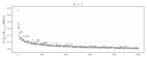
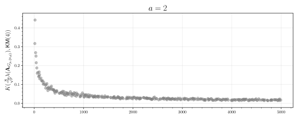
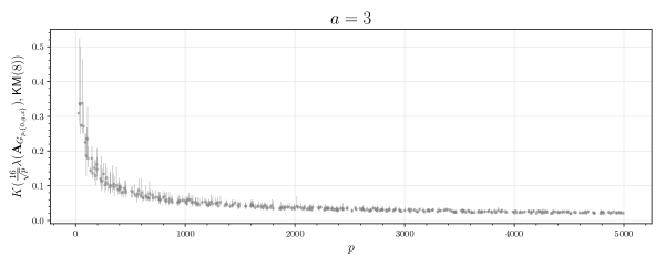
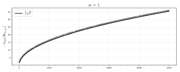
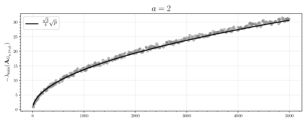
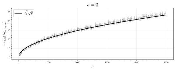
If an explicit error term is obtained in Conjecture 1.9, then the o(p)𝑜𝑝o(\sqrt{p}) term may be made explicit as well. Unfortunately, as we discuss in Section 7, we believe proving Conjecture 1.9 at degree a2𝑎2a\geq 2 will be significantly harder than proving Conjecture 1.8. But, in Section 8, we give numerical evidence for both Conjectures 1.8 and 1.9 at low degrees.

Let us compare Theorem 1.19 with the state-of-the-art bound of Hanson and Petridis (our Theorem 1.2). The latter scales as 22p0.707p22𝑝0.707𝑝\frac{\sqrt{2}}{2}\sqrt{p}\approx 0.707\sqrt{p}. For a=1𝑎1a=1 the bound of Theorem 1.19 scales as p𝑝\sqrt{p}, the “trivial” bound (see Remark 5.2 for an explanation). For a=2𝑎2a=2 our bound would scale as 32p0.866p32𝑝0.866𝑝\frac{\sqrt{3}}{2}\sqrt{p}\approx 0.866\sqrt{p}, in between the trivial bound and the Hanson-Petridis bound. But, already for a=3𝑎3a=3 our bound would scale as 74p0.661p74𝑝0.661𝑝\frac{\sqrt{7}}{4}\sqrt{p}\approx 0.661\sqrt{p}, improving on the Hanson-Petridis bound. Moreover, if Conjecture 1.9 held for arbitrarily large a𝑎a, then our bound would show that ω(Gp)=o(p)𝜔subscript𝐺𝑝𝑜𝑝\omega(G_{p})=o(\sqrt{p}), and taking a=a(p)𝑎𝑎𝑝a=a(p) growing slowly should allow explicit improvements on the p𝑝\sqrt{p} scaling using the same proof strategy.

1.7 Related work

Constructive Ramsey theory

The diagonal Ramsey number R(k)𝑅𝑘R(k) is the maximum of |V(G)|𝑉𝐺|V(G)| over graphs G𝐺G with ω(G)k𝜔𝐺𝑘\omega(G)\leq k and α(G)k𝛼𝐺𝑘\alpha(G)\leq k. Ramsey’s famous theorem initiating Ramsey theory [Ram29] gives a finite upper bound on R(k)𝑅𝑘R(k), and it has since been of great interest in combinatorics to prove tighter bounds on R(k)𝑅𝑘R(k). By showing that G𝐺G an ER graph on p𝑝p vertices has max{ω(G),α(G)}2log2p𝜔𝐺𝛼𝐺2subscript2𝑝\max\{\omega(G),\alpha(G)\}\leq 2\log_{2}p with positive probability, Erdős [Erd47] showed, in an early use of the probabilistic method (see, e.g., [Spe94]), that R(k)2k/2𝑅𝑘superscript2𝑘2R(k)\geq 2^{k/2}. It is a long-standing open problem to match this result with an explicit construction, and the Paley graph is perhaps the main candidate for such a graph.666It is also a long-standing open problem to prove matching upper and lower bounds on R(k)𝑅𝑘R(k); the main result of [ES35] is that R(k)4k𝑅𝑘superscript4𝑘R(k)\leq 4^{k}, and the recent breakthrough [CGMS23] for the first time improves the base of the exponent. The best known results [Coh16, CZ16] give deterministic constructions of G𝐺G on p𝑝p vertices with max{ω(G),α(G)}exp((loglogp)C)𝜔𝐺𝛼𝐺superscript𝑝𝐶\max\{\omega(G),\alpha(G)\}\leq\exp((\log\log p)^{C}) for some C>0𝐶0C>0.777Equivalently, this is a deterministic construction for R(k)exp(exp((logk)c))𝑅𝑘superscript𝑘𝑐R(k)\geq\exp(\exp((\log k)^{c})) for some c>0𝑐0c>0, while Conjecture 1.1 would give that the Paley graph is a deterministic construction for R(k)exp(kc)𝑅𝑘superscript𝑘𝑐R(k)\geq\exp(k^{c}) for some c>0𝑐0c>0. Note also that the consequence ω(Gp)=α(Gp)=o(p)𝜔subscript𝐺𝑝𝛼subscript𝐺𝑝𝑜𝑝\omega(G_{p})=\alpha(G_{p})=o(\sqrt{p}) of our conjectures would not improve on this result; much stronger sub-polynomial clique number bounds would be required for that. See, e.g., [Wig19, Sections 8.2 and 9] or [Vad12] for more discussion and consequences of such constructions for the theory of algorithms.

Generic clique number bounds

We have restricted our attention to combining localization with general-purpose convex relaxation bounds on the clique (or independence) number. There are many variations of such bounds known, including spectral [Hof70, Hae95, GN08, BT19, Hae21], LP [Del72, Del73, Sch79, SA90], and SDP [Lov79, Knu93, Lov03, Lau03, Las01, Par03] bounds (we include references for bounds on the chromatic number as well, which are typically similar in spirit). There is also another class of rank or inertia bounds, which instead only work with the number of positive, negative, and zero eigenvalues of suitable matrices, e.g., [Hae78, GR01, Sin18]. It is an interesting question to consider how these other bounds interact with localization.

Paley graph clique number bounds

The history of upper bounds on ω(Gp)𝜔subscript𝐺𝑝\omega(G_{p}) is brief: the p𝑝\sqrt{p} bound has long been folklore and admits an elementary combinatorial proof [Yip22, Lemma 1.2]. The first improvements [MP06, BMR13] showed a bound of p1𝑝1\sqrt{p}-1 under different conditions on p𝑝p. The state-of-the-art result of [HP21] was also the first to improve the constant in front of p𝑝\sqrt{p}, using the polynomial method, and [DBSW21] gave an alternate proof soon after. The lower bounds we mention in the introduction are number-theoretic improvements of the bound ω(Gp)(12+o(1))log2p𝜔subscript𝐺𝑝12𝑜1subscript2𝑝\omega(G_{p})\geq(\frac{1}{2}+o(1))\log_{2}p which follows from the general upper bound on the Ramsey number R(k)𝑅𝑘R(k) due to [ES35] and the fact that ω(Gp)=α(Gp)𝜔subscript𝐺𝑝𝛼subscript𝐺𝑝\omega(G_{p})=\alpha(G_{p}).

Explicit semicircular elements

Some recent work has pursued constructing explicit deterministic matrices whose e.s.d. is close (in some distributional distance such as Kolmogorov distance; see our Definition 8.1) to the semicircle law [SXT17, SXT18]. Since, after rescaling, the Kesten-McKay measures 𝖪𝖬(v)𝖪𝖬𝑣\mathsf{KM}(v) approach the semicircle law as v𝑣v\to\infty, our results suggest that any sequence of adjacency matrices 𝑨Gp,Isubscript𝑨subscript𝐺𝑝𝐼\bm{A}_{G_{p,I}} or 𝑺Gp,Isubscript𝑺subscript𝐺𝑝𝐼\bm{S}_{G_{p,I}} for Ia(Gp)𝐼subscript𝑎subscript𝐺𝑝I\in\mathcal{I}_{a}(G_{p}) with a=a(p)𝑎𝑎𝑝a=a(p)\to\infty should be good candidates for such constructions, but we do not pursue a careful analysis here.

Deterministic asymptotic freeness

We will see that our Conjecture 1.8 follows from Conjecture 4.1, which posits that certain explicit deterministic pairs of projection matrices are asymptotically free. We are not aware of many examples of deterministic asymptotically free pairs, particularly not for pairs of projections as in our case. One such example is given in [CVVE12, Example 9], and another for deterministic matrices with e.s.d. converging to the semicircle law as discussed above in [ST18]. Generally, it is an interesting problem to derandomize classical results of free probability, finding deterministic pairs of matrices under various restrictions that are asymptotically free.

Character sum estimates

Though necklace character sums can be written in the standard form 𝒙𝔽pkχ(q(𝒙))subscript𝒙superscriptsubscript𝔽𝑝𝑘𝜒𝑞𝒙\sum_{\bm{x}\in\mathbb{F}_{p}^{k}}\chi(q(\bm{x})) for q𝑞q a polynomial, we are not aware of any general purpose character sum estimates that treat our particular q𝑞q (see [IK21] for a broad survey of the area; some results that handle situations similar to ours include [Kat99, RL05, Kat07, Kat08]). The issue is that q(𝒙)𝑞𝒙q(\bm{x}) is highly “singular,” in the sense that the variety {𝒙:q(𝒙)=0}𝔽pkconditional-set𝒙𝑞𝒙0superscriptsubscript𝔽𝑝𝑘\{\bm{x}:q(\bm{x})=0\}\subseteq\mathbb{F}_{p}^{k} is highly singular, since q𝑞q is a product of linear factors. A very similar situation is treated in the recent work [RL22], but unfortunately its assumptions still ask for the linear factors of q𝑞q to be in a “general position” that our setting does not satisfy. We also point out the reference [Chu89], which uses simpler character sum estimates to control the spectrum of a different pseudorandom graph construction.

2 Notation

We write 𝑰nn×nsubscript𝑰𝑛superscript𝑛𝑛\bm{I}_{n}\in\mathbb{R}^{n\times n} for the identity matrix of corresponding dimension. We write 𝟏𝔽p1superscriptsubscript𝔽𝑝\bm{1}\in\mathbb{R}^{\mathbb{F}_{p}} for the all-ones vector, and 𝟏^\colonequals1p𝟏^1\colonequals1𝑝1\widehat{\bm{1}}\colonequals\frac{1}{\sqrt{p}}\bm{1}, so that 𝟏^=1norm^11\|\widehat{\bm{1}}\|=1. We write 𝒆1,,𝒆nnsubscript𝒆1subscript𝒆𝑛superscript𝑛\bm{e}_{1},\dots,\bm{e}_{n}\in\mathbb{R}^{n} for the standard orthonormal basis, with (𝒆i)j=1{i=j}subscriptsubscript𝒆𝑖𝑗1𝑖𝑗(\bm{e}_{i})_{j}=\mathbbold{1}\{i=j\}. For I[n]𝐼delimited-[]𝑛I\subseteq[n], we write 𝑬I=iI𝒆i𝒆isubscript𝑬𝐼subscript𝑖𝐼subscript𝒆𝑖superscriptsubscript𝒆𝑖top\bm{E}_{I}=\sum_{i\in I}\bm{e}_{i}\bm{e}_{i}^{\top}. Matrix multiplications bind before the trace, so Tr𝑨𝑩=Tr(𝑨𝑩)Tr𝑨𝑩Tr𝑨𝑩\operatorname{Tr}\bm{A}\bm{B}=\operatorname{Tr}(\bm{A}\bm{B}) and Tr(𝑨𝑩)k=Tr((𝑨𝑩)k)\operatorname{Tr}(\bm{A}\bm{B})^{k}=\operatorname{Tr}((\bm{A}\bm{B})^{k}). For 𝑨symn×n𝑨subscriptsuperscript𝑛𝑛sym\bm{A}\in\mathbb{R}^{n\times n}_{\operatorname{sym}}, we write λ1(𝑨)λn(𝑨)subscript𝜆1𝑨subscript𝜆𝑛𝑨\lambda_{1}(\bm{A})\geq\cdots\geq\lambda_{n}(\bm{A}) for the ordered (real) eigenvalues. We also write λmax(𝑨)\colonequalsλ1(𝑨)subscript𝜆𝑨\colonequalssubscript𝜆1𝑨\lambda_{\max}(\bm{A})\colonequals\lambda_{1}(\bm{A}) and λmin(𝑨)\colonequalsλn(𝑨)subscript𝜆𝑨\colonequalssubscript𝜆𝑛𝑨\lambda_{\min}(\bm{A})\colonequals\lambda_{n}(\bm{A}). For 𝑨m×n𝑨superscript𝑚𝑛\bm{A}\in\mathbb{R}^{m\times n}, we write 𝑨norm𝑨\|\bm{A}\| for the operator norm or largest singular value, 𝑨F=Tr(𝑨𝑨)subscriptnorm𝑨𝐹Tr𝑨superscript𝑨top\|\bm{A}\|_{F}=\sqrt{\operatorname{Tr}(\bm{A}\bm{A}^{\top})} for the Frobenius norm, and 𝑨=Tr(𝑨𝑨)subscriptnorm𝑨Tr𝑨superscript𝑨top\|\bm{A}\|_{*}=\operatorname{Tr}(\sqrt{\bm{A}\bm{A}^{\top}}) for the nuclear norm.

For a graph G𝐺G, we write V(G)𝑉𝐺V(G) for the vertex set, deg(v)degree𝑣\deg(v) for the degree of vV(G)𝑣𝑉𝐺v\in V(G), and mindeg(G)degree𝐺\min\deg(G) and maxdeg(G)degree𝐺\max\deg(G) for the minimum and maximum degree of any vertex in G𝐺G, respectively. We write 𝑨Gsubscript𝑨𝐺\bm{A}_{G} for the {0,1}01\{0,1\}-valued adjacency matrix, and 𝑺G=2𝑨G𝟏𝟏+𝑰subscript𝑺𝐺2subscript𝑨𝐺superscript11top𝑰\bm{S}_{G}=2\bm{A}_{G}-\bm{1}\bm{1}^{\top}+\bm{I} for the {±1}plus-or-minus1\{\pm 1\}-valued adjacency matrix.

All asymptotic notations O(),o(),ω(),Ω(),Θ(),,𝑂𝑜𝜔ΩΘmuch-less-thanmuch-greater-thanO(\cdot),o(\cdot),\omega(\cdot),\Omega(\cdot),\Theta(\cdot),\ll,\gg refer to the limit of p𝑝p\to\infty over primes p1(mod 4)𝑝1mod4p\equiv 1\ (\mathrm{mod}\ 4). Subscripts such as Oa()subscript𝑂𝑎O_{a}(\cdot) denote which parameters the implicit constant depends on.

We reserve χ𝜒\chi for the Legendre symbol, ε𝜀\varepsilon for the trivial character, and ϕ,ψitalic-ϕ𝜓\phi,\psi for general multiplicative characters of 𝔽p×superscriptsubscript𝔽𝑝\mathbb{F}_{p}^{\times}. We write 𝔽p×^^superscriptsubscript𝔽𝑝\widehat{\mathbb{F}_{p}^{\times}} for the dual group, the set of all multiplicative characters. We write ϕ¯¯italic-ϕ\overline{\phi} for the conjugate character ϕ¯(x)=ϕ(x)¯¯italic-ϕ𝑥¯italic-ϕ𝑥\overline{\phi}(x)=\overline{\phi(x)}, and write ϕψitalic-ϕ𝜓\phi\psi for pointwise multiplication, so that ϕψ(x)=ϕ(x)ψ(x)italic-ϕ𝜓𝑥italic-ϕ𝑥𝜓𝑥\phi\psi(x)=\phi(x)\psi(x).

3 Preliminaries

3.1 Paley graphs

We recall a few basic and well-known properties of the Paley graph.

Proposition 3.1 (Automorphisms).

Let σa,b:𝔽p𝔽p:subscript𝜎𝑎𝑏subscript𝔽𝑝subscript𝔽𝑝\sigma_{a,b}:\mathbb{F}_{p}\to\mathbb{F}_{p} be given by σa,b(x)=ax+bsubscript𝜎𝑎𝑏𝑥𝑎𝑥𝑏\sigma_{a,b}(x)=ax+b. Then, {σa,b}aSSp,b𝔽psubscriptsubscript𝜎𝑎𝑏formulae-sequence𝑎subscriptSS𝑝𝑏subscript𝔽𝑝\{\sigma_{a,b}\}_{a\in\SS_{p},b\in\mathbb{F}_{p}} is the automorphism group of Gpsubscript𝐺𝑝G_{p}, having size p(p1)2𝑝𝑝12\frac{p(p-1)}{2}.

Corollary 3.2 (Transitivity).

There exists an automorphism of Gpsubscript𝐺𝑝G_{p} mapping any vertex to any other vertex (i.e., Gpsubscript𝐺𝑝G_{p} is vertex transitive), mapping any edge to any edge (i.e., Gpsubscript𝐺𝑝G_{p} is edge transitive), and any non-edge to any non-edge (i.e., Gp¯¯subscript𝐺𝑝\overline{G_{p}} is edge transitive).

Proposition 3.3 (Spectral decomposition).

Define matrices 𝐏p(±)sym𝔽p×𝔽psubscriptsuperscript𝐏plus-or-minus𝑝subscriptsuperscriptsubscript𝔽𝑝subscript𝔽𝑝sym\bm{P}^{(\pm)}_{p}\in\mathbb{R}^{\mathbb{F}_{p}\times\mathbb{F}_{p}}_{\operatorname{sym}} to have entries

(𝑷p(+))ijsubscriptsubscriptsuperscript𝑷𝑝𝑖𝑗\displaystyle(\bm{P}^{(+)}_{p})_{ij} \colonequals{p12pif i=j,p12pif ij and iGpj,p+12pif ij and i≁Gpj,\colonequalscases𝑝12𝑝if 𝑖𝑗𝑝12𝑝if 𝑖𝑗 and 𝑖subscriptsimilar-tosubscript𝐺𝑝𝑗𝑝12𝑝if 𝑖𝑗 and 𝑖subscriptnot-similar-tosubscript𝐺𝑝𝑗\displaystyle\colonequals\left\{\begin{array}[]{rl}\frac{p-1}{2p}&\text{if }i=j,\\ \frac{\sqrt{p}-1}{2p}&\text{if }i\neq j\text{ and }i\sim_{G_{p}}j,\\ -\frac{\sqrt{p}+1}{2p}&\text{if }i\neq j\text{ and }i\not\sim_{G_{p}}j,\end{array}\right. (25)
(𝑷p())ijsubscriptsubscriptsuperscript𝑷𝑝𝑖𝑗\displaystyle(\bm{P}^{(-)}_{p})_{ij} \colonequals{p12pif i=j,p+12pif ij and iGpj,p12pif ij and i≁Gpj.\colonequalscases𝑝12𝑝if 𝑖𝑗𝑝12𝑝if 𝑖𝑗 and 𝑖subscriptsimilar-tosubscript𝐺𝑝𝑗𝑝12𝑝if 𝑖𝑗 and 𝑖subscriptnot-similar-tosubscript𝐺𝑝𝑗\displaystyle\colonequals\left\{\begin{array}[]{rl}\frac{p-1}{2p}&\text{if }i=j,\\ -\frac{\sqrt{p}+1}{2p}&\text{if }i\neq j\text{ and }i\sim_{G_{p}}j,\\ \frac{\sqrt{p}-1}{2p}&\text{if }i\neq j\text{ and }i\not\sim_{G_{p}}j.\end{array}\right. (29)

Then, 𝐏p(±)subscriptsuperscript𝐏plus-or-minus𝑝\bm{P}^{(\pm)}_{p} are orthogonal projections, each has rank (p1)/2𝑝12(p-1)/2, and these matrices satisfy

𝟏^𝟏^+𝑷p(+)+𝑷p()=𝑰𝔽p.^1superscript^1topsubscriptsuperscript𝑷𝑝subscriptsuperscript𝑷𝑝subscript𝑰subscript𝔽𝑝\widehat{\bm{1}}\widehat{\bm{1}}^{\top}+\bm{P}^{(+)}_{p}+\bm{P}^{(-)}_{p}=\bm{I}_{\mathbb{F}_{p}}. (30)

The {0,1}01\{0,1\} and {±1}plus-or-minus1\{\pm 1\} adjacency matrices of Gpsubscript𝐺𝑝G_{p} then admit the following spectral decompositions:

𝑨Gpsubscript𝑨subscript𝐺𝑝\displaystyle\bm{A}_{G_{p}} =p12𝟏^𝟏^+p12𝑷p(+)p+12𝑷p(),absent𝑝12^1superscript^1top𝑝12subscriptsuperscript𝑷𝑝𝑝12subscriptsuperscript𝑷𝑝\displaystyle=\frac{p-1}{2}\widehat{\bm{1}}\,\widehat{\bm{1}}^{\top}+\frac{\sqrt{p}-1}{2}\bm{P}^{(+)}_{p}-\frac{\sqrt{p}+1}{2}\bm{P}^{(-)}_{p}, (31)
𝑺Gpsubscript𝑺subscript𝐺𝑝\displaystyle\bm{S}_{G_{p}} =2𝑨Gp𝟏𝟏+𝑰𝔽pabsent2subscript𝑨subscript𝐺𝑝superscript11topsubscript𝑰subscript𝔽𝑝\displaystyle=2\bm{A}_{G_{p}}-\bm{1}\bm{1}^{\top}+\bm{I}_{\mathbb{F}_{p}}
=p𝑷p(+)p𝑷p().absent𝑝superscriptsubscript𝑷𝑝𝑝subscriptsuperscript𝑷𝑝\displaystyle=\sqrt{p}\,\bm{P}_{p}^{(+)}-\sqrt{p}\,\bm{P}^{(-)}_{p}. (32)

3.2 Number theory

We next gather several number-theoretic facts that we will need. We adopt the standard notation

ep(x)\colonequalsexp(2πipx).subscript𝑒𝑝𝑥\colonequals2𝜋𝑖𝑝𝑥e_{p}(x)\colonequals\exp\left(\frac{2\pi i}{p}x\right). (33)
Definition 3.4 (Multiplicative characters).

We write 𝔽p×^^superscriptsubscript𝔽𝑝\widehat{\mathbb{F}_{p}^{\times}} for the group of multiplicative characters on 𝔽psubscript𝔽𝑝\mathbb{F}_{p}. Recall that |𝔽p×^|=p1^superscriptsubscript𝔽𝑝𝑝1|\widehat{\mathbb{F}_{p}^{\times}}|=p-1, and this group is isomorphic to the cyclic group of order p1𝑝1p-1. We write χ𝔽p×^𝜒^superscriptsubscript𝔽𝑝\chi\in\widehat{\mathbb{F}_{p}^{\times}} for the Legendre symbol and ε𝔽p×^𝜀^superscriptsubscript𝔽𝑝\varepsilon\in\widehat{\mathbb{F}_{p}^{\times}} for the trivial character. We extend characters ψ𝜓\psi to have domain 𝔽psubscript𝔽𝑝\mathbb{F}_{p} (including zero) by setting ψ(0)\colonequals0𝜓0\colonequals0\psi(0)\colonequals 0 for all ψ𝜓\psi (including setting ε(0)\colonequals0𝜀0\colonequals0\varepsilon(0)\colonequals 0, which is a common but not universal convention).

Definition 3.5 (Character sums).

The Gauss, Jacobi, and Kloosterman sums are defined as, respectively,

G(ψ)𝐺𝜓\displaystyle G(\psi) \colonequalsx𝔽pψ(x)ep(x),\colonequalssubscript𝑥subscript𝔽𝑝𝜓𝑥subscript𝑒𝑝𝑥\displaystyle\colonequals\sum_{x\in\mathbb{F}_{p}}\psi(x)e_{p}(x), (34)
J(ψ,ϕ)𝐽𝜓italic-ϕ\displaystyle J(\psi,\phi) \colonequalsx𝔽pψ(x)ϕ(1x),\colonequalssubscript𝑥subscript𝔽𝑝𝜓𝑥italic-ϕ1𝑥\displaystyle\colonequals\sum_{x\in\mathbb{F}_{p}}\psi(x)\phi(1-x), (35)
Kk(a)subscript𝐾𝑘𝑎\displaystyle K_{k}(a) \colonequalsx1,,xk𝔽px1xk=aep(x1++xk),\colonequalssubscriptsubscript𝑥1subscript𝑥𝑘subscript𝔽𝑝subscript𝑥1subscript𝑥𝑘𝑎subscript𝑒𝑝subscript𝑥1subscript𝑥𝑘\displaystyle\colonequals\sum_{\begin{subarray}{c}x_{1},\dots,x_{k}\in\mathbb{F}_{p}\\ x_{1}\cdots x_{k}=a\end{subarray}}e_{p}(x_{1}+\cdots+x_{k}), (36)

for ψ,ϕ𝔽p×^𝜓italic-ϕ^superscriptsubscript𝔽𝑝\psi,\phi\in\widehat{\mathbb{F}_{p}^{\times}} and a𝔽p×𝑎superscriptsubscript𝔽𝑝a\in\mathbb{F}_{p}^{\times}.

The following results may be viewed as Fourier transforms of various functions on either the additive group 𝔽psubscript𝔽𝑝\mathbb{F}_{p} or the multiplicative group 𝔽p×superscriptsubscript𝔽𝑝\mathbb{F}_{p}^{\times}. There are many interesting identities of this kind connecting various exponential and character sums; the reader may consult, for instance, [Kat88, p. 47].

Proposition 3.6.

For all x𝔽p𝑥subscript𝔽𝑝x\in\mathbb{F}_{p},

χ(x)𝜒𝑥\displaystyle\chi(x) =1pa𝔽pχ(a)ep(ax),absent1𝑝subscript𝑎subscript𝔽𝑝𝜒𝑎subscript𝑒𝑝𝑎𝑥\displaystyle=\frac{1}{\sqrt{p}}\sum_{a\in\mathbb{F}_{p}}\chi(a)e_{p}(ax), (37)
1{x=1}1𝑥1\displaystyle\mathbbold{1}\{x=1\} =1p1ψ𝔽p×^ψ(x).absent1𝑝1subscript𝜓^superscriptsubscript𝔽𝑝𝜓𝑥\displaystyle=\frac{1}{p-1}\sum_{\psi\in\widehat{\mathbb{F}_{p}^{\times}}}\psi(x). (38)

Character sum estimates

The following is the main powerful theorem controlling univariate character sums.

Theorem 3.7 (Weil’s bound, Chapter 11 of [IK21]).

Let q𝔽p[t]𝑞subscript𝔽𝑝delimited-[]𝑡q\in\mathbb{F}_{p}[t] have degq=ddegree𝑞𝑑\deg q=d. Suppose that q𝑞q cannot be represented as q(t)=cr(t)2𝑞𝑡𝑐𝑟superscript𝑡2q(t)=c\cdot r(t)^{2} for c𝔽p𝑐subscript𝔽𝑝c\in\mathbb{F}_{p} and r𝔽p[t]𝑟subscript𝔽𝑝delimited-[]𝑡r\in\mathbb{F}_{p}[t]. Then,

|x𝔽pχ(q(x))|(d1)p.subscript𝑥subscript𝔽𝑝𝜒𝑞𝑥𝑑1𝑝\left|\sum_{x\in\mathbb{F}_{p}}\chi(q(x))\right|\leq(d-1)\sqrt{p}. (39)

We refer to a sum as on the left-hand side of (39) as a Weil sum.

It turns out to be possible to evaluate the magnitude of any Gauss sum, as follows.

Proposition 3.8 ([IR90, Sections 6.4 and 8.2]).

G(ε)=1𝐺𝜀1G(\varepsilon)=-1, and |G(ψ)|=p𝐺𝜓𝑝|G(\psi)|=\sqrt{p} for all ψε𝜓𝜀\psi\neq\varepsilon. Moreover, G(χ)=p𝐺𝜒𝑝G(\chi)=\sqrt{p} for all p1(mod 4)𝑝1mod4p\equiv 1\ (\mathrm{mod}\ 4).

Because of this uniformity of the magnitude, other interesting properties of Gauss sums are often stated in terms of the complex modulus or “angle,”

g(ψ)\colonequalsG(ψ)p for ψε.𝑔𝜓\colonequals𝐺𝜓𝑝 for 𝜓𝜀g(\psi)\colonequals\frac{G(\psi)}{\sqrt{p}}\text{ for }\psi\neq\varepsilon. (40)

The main intuition about these quantities is that they behave, when taken over all ψ𝜓\psi, as though randomly distributed on the complex unit circle. The following deep result of Katz quantifies this pseudorandomness or “equidistribution.”

Theorem 3.9 ([Kat88, Theorem 9.6]).

For any ϕ1,,ϕr𝔽p×^subscriptitalic-ϕ1subscriptitalic-ϕ𝑟^superscriptsubscript𝔽𝑝\phi_{1},\dots,\phi_{r}\in\widehat{\mathbb{F}_{p}^{\times}} distinct and m1,,mrsubscript𝑚1subscript𝑚𝑟m_{1},\dots,m_{r}\in\mathbb{Z},

|ψ𝔽p×^{ϕ1¯,,ϕr¯}g(ϕ1ψ)m1g(ϕrψ)mr|(i=1r|mi|)p+2r.subscript𝜓^superscriptsubscript𝔽𝑝¯subscriptitalic-ϕ1¯subscriptitalic-ϕ𝑟𝑔superscriptsubscriptitalic-ϕ1𝜓subscript𝑚1𝑔superscriptsubscriptitalic-ϕ𝑟𝜓subscript𝑚𝑟superscriptsubscript𝑖1𝑟subscript𝑚𝑖𝑝2𝑟\left|\sum_{\psi\in\widehat{\mathbb{F}_{p}^{\times}}\setminus\{\overline{\phi_{1}},\dots,\overline{\phi_{r}}\}}g(\phi_{1}\psi)^{m_{1}}\cdots g(\phi_{r}\psi)^{m_{r}}\right|\leq\left(\sum_{i=1}^{r}|m_{i}|\right)\sqrt{p}+2r. (41)

We emphasize the remarkable simplicity and non-asymptotic form of this result—this is thanks to the powerful algebraic-geometric machinery developed for character sum estimates in analytic number theory. See [IK21, Chapter 21] for some further discussion of such equidistribution results.

It is also possible to reduce the problem of evaluating Jacobi sums to that of evaluating Gauss sums.

Proposition 3.10 ([IR90, Section 8.3]).

Let ϕ,ψ𝔽p×^italic-ϕ𝜓^superscriptsubscript𝔽𝑝\phi,\psi\in\widehat{\mathbb{F}_{p}^{\times}}. Then,

J(ϕ,ψ)={p2if ϕ=ψ=ε,0if exactly one of ϕ,ψ is ε,ϕ(1)if ϕψ=ε and ϕ,ψε,G(ϕ)G(ψ)/G(ϕψ)if ϕ,ψ,ϕψε.𝐽italic-ϕ𝜓cases𝑝2if italic-ϕ𝜓𝜀0if exactly one of italic-ϕ𝜓 is 𝜀italic-ϕ1formulae-sequenceif italic-ϕ𝜓𝜀 and italic-ϕ𝜓𝜀𝐺italic-ϕ𝐺𝜓𝐺italic-ϕ𝜓if italic-ϕ𝜓italic-ϕ𝜓𝜀J(\phi,\psi)=\left\{\begin{array}[]{ll}p-2&\text{if }\phi=\psi=\varepsilon,\\ 0&\text{if exactly one of }\phi,\psi\text{ is }\varepsilon,\\ -\phi(-1)&\text{if }\phi\psi=\varepsilon\text{ and }\phi,\psi\neq\varepsilon,\\ G(\phi)G(\psi)/G(\phi\psi)&\text{if }\phi,\psi,\phi\psi\neq\varepsilon.\end{array}\right. (42)

We will use below that, through Katz’s bound, this allows us to quantify cancellations in sums of polynomials of Jacobi sums (taken over multiplicative characters).

Similar results are also known for Kloosterman sums; the following result on “moments” of Kloosterman sums (in the same sense as above of a sum of monomials) that are “twisted” by a character is the one we will use. For Kloosterman sums, even controlling the magnitude |Kk(x)|subscript𝐾𝑘𝑥|K_{k}(x)| is a deep result of Weil for k=2𝑘2k=2 and of Deligne for general k𝑘k (see [DGIV77] or [IK21, Chapter 11]), who showed that

|Kk(x)|kpk12.subscript𝐾𝑘𝑥𝑘superscript𝑝𝑘12|K_{k}(x)|\leq kp^{\frac{k-1}{2}}. (43)

In light of this, the following should be viewed as describing square root cancellations in moments of Kloosterman sums.

Theorem 3.11 ([LZZ18, Lemma 2.1]).

Let ψ𝔽p×^𝜓^superscriptsubscript𝔽𝑝\psi\in\widehat{\mathbb{F}_{p}^{\times}} be non-trivial, k1𝑘1k\geq 1, and r,s0𝑟𝑠0r,s\geq 0. Then,

|x𝔽p×ψ(x)Kk(x)rKk(x)¯s|kr+s1p(k1)(r+s)+12.subscript𝑥superscriptsubscript𝔽𝑝𝜓𝑥subscript𝐾𝑘superscript𝑥𝑟superscript¯subscript𝐾𝑘𝑥𝑠superscript𝑘𝑟𝑠1superscript𝑝𝑘1𝑟𝑠12\left|\sum_{x\in\mathbb{F}_{p}^{\times}}\psi(x)K_{k}(x)^{r}\overline{K_{k}(x)}^{s}\right|\leq k^{r+s-1}p^{\frac{(k-1)(r+s)+1}{2}}. (44)

Similar results for the k=2𝑘2k=2 case of Kloosterman sums are obtained in [Liu02] and [CI00].

3.3 Weak convergence and asymptotic freeness

The following is a standard folklore “robustness” statement for weak convergence. We will use this to allow ourselves to ignore various corrections involved in translating between the {0,1}01\{0,1\} adjacency matrix of Gpsubscript𝐺𝑝G_{p}, the {±1}plus-or-minus1\{\pm 1\} adjacency matrix of Gpsubscript𝐺𝑝G_{p}, and the projection matrices 𝑷p(±)superscriptsubscript𝑷𝑝plus-or-minus\bm{P}_{p}^{(\pm)} discussed above.

Proposition 3.12.

Suppose 𝐀(N),𝐁(N)symN×Nsuperscript𝐀𝑁superscript𝐁𝑁subscriptsuperscript𝑁𝑁sym\bm{A}^{(N)},\bm{B}^{(N)}\in\mathbb{R}^{N\times N}_{\operatorname{sym}} for N=N(n)𝑁𝑁𝑛N=N(n) an increasing sequence are matrices such that 1Nj=1Nδλj(𝐀(N))1𝑁superscriptsubscript𝑗1𝑁subscript𝛿subscript𝜆𝑗superscript𝐀𝑁\frac{1}{N}\sum_{j=1}^{N}\delta_{\lambda_{j}(\bm{A}^{(N)})} converges weakly to a probability measure ρ𝜌\rho supported on [C,C]𝐶𝐶[-C,C]\subset\mathbb{R} for some C>0𝐶0C>0 as n𝑛n\to\infty and 𝐀(N)𝐁(N)/N0subscriptnormsuperscript𝐀𝑁superscript𝐁𝑁𝑁0\|\bm{A}^{(N)}-\bm{B}^{(N)}\|_{*}/N\to 0 as n𝑛n\to\infty. Then, 1Nj=1Nδλj(𝐁(N))1𝑁superscriptsubscript𝑗1𝑁subscript𝛿subscript𝜆𝑗superscript𝐁𝑁\frac{1}{N}\sum_{j=1}^{N}\delta_{\lambda_{j}(\bm{B}^{(N)})} converges weakly to ρ𝜌\rho as well.

Proof.

We will use the 1superscript1\ell^{1} version of the Hoffman-Wielandt inequality [Bha13, Theorem III.4.4], which gives

limN1Nj=1N|λj(𝑨(N))λj(𝑩(N))|limN1N𝑨(N)𝑩(N)=0.subscript𝑁1𝑁superscriptsubscript𝑗1𝑁subscript𝜆𝑗superscript𝑨𝑁subscript𝜆𝑗superscript𝑩𝑁subscript𝑁1𝑁subscriptnormsuperscript𝑨𝑁superscript𝑩𝑁0\lim_{N\to\infty}\frac{1}{N}\sum_{j=1}^{N}|\lambda_{j}(\bm{A}^{(N)})-\lambda_{j}(\bm{B}^{(N)})|\leq\lim_{N\to\infty}\frac{1}{N}\|\bm{A}^{(N)}-\bm{B}^{(N)}\|_{*}=0. (45)

By our assumption on ρ𝜌\rho, we have

limN#{j:λj(𝑨(N))[2C,2C]}N=0,subscript𝑁#conditional-set𝑗subscript𝜆𝑗superscript𝑨𝑁2𝐶2𝐶𝑁0\lim_{N\to\infty}\frac{\#\{j:\lambda_{j}(\bm{A}^{(N)})\notin[-2C,2C]\}}{N}=0, (46)

and thus

limN#{j:λj(𝑩(N))[3C,3C]}N=0.subscript𝑁#conditional-set𝑗subscript𝜆𝑗superscript𝑩𝑁3𝐶3𝐶𝑁0\lim_{N\to\infty}\frac{\#\{j:\lambda_{j}(\bm{B}^{(N)})\notin[-3C,3C]\}}{N}=0. (47)

Now, let h::h:\mathbb{R}\to\mathbb{R} be a bounded smooth function, and let L\colonequalsmaxx[3C,3C]|h(x)|<𝐿\colonequalssubscript𝑥3𝐶3𝐶superscript𝑥L\colonequals\max_{x\in[-3C,3C]}|h^{\prime}(x)|<\infty and M\colonequalssupx|h(x)|𝑀\colonequalssubscriptsupremum𝑥𝑥M\colonequals\sup_{x\in\mathbb{R}}|h(x)|. Then,

|1Nj=1Nh(λj(𝑨(N)))1Nj=1Nh(λj(𝑩(N)))|1𝑁superscriptsubscript𝑗1𝑁subscript𝜆𝑗superscript𝑨𝑁1𝑁superscriptsubscript𝑗1𝑁subscript𝜆𝑗superscript𝑩𝑁\displaystyle\left|\frac{1}{N}\sum_{j=1}^{N}h(\lambda_{j}(\bm{A}^{(N)}))-\frac{1}{N}\sum_{j=1}^{N}h(\lambda_{j}(\bm{B}^{(N)}))\right|
1Nj=1N|h(λj(𝑨(N)))h(λj(𝑩(N)))|absent1𝑁superscriptsubscript𝑗1𝑁subscript𝜆𝑗superscript𝑨𝑁subscript𝜆𝑗superscript𝑩𝑁\displaystyle\leq\frac{1}{N}\sum_{j=1}^{N}|h(\lambda_{j}(\bm{A}^{(N)}))-h(\lambda_{j}(\bm{B}^{(N)}))|
LNj=1N|λj(𝑨(N))λj(𝑩(N))|absent𝐿𝑁superscriptsubscript𝑗1𝑁subscript𝜆𝑗superscript𝑨𝑁subscript𝜆𝑗superscript𝑩𝑁\displaystyle\leq\frac{L}{N}\sum_{j=1}^{N}|\lambda_{j}(\bm{A}^{(N)})-\lambda_{j}(\bm{B}^{(N)})|
+MN(#{j:λj(𝑨(N))[3C,3C]}+#{j:λj(𝑩(N))[3C,3C]}).𝑀𝑁#conditional-set𝑗subscript𝜆𝑗superscript𝑨𝑁3𝐶3𝐶#conditional-set𝑗subscript𝜆𝑗superscript𝑩𝑁3𝐶3𝐶\displaystyle\hskip 28.45274pt+\frac{M}{N}\big{(}\#\{j:\lambda_{j}(\bm{A}^{(N)})\notin[-3C,3C]\}+\#\{j:\lambda_{j}(\bm{B}^{(N)})\notin[-3C,3C]\}\big{)}. (48)

Both terms on the right-hand side tend to zero by our observations above. The result follows by a standard approximation argument since this holds for any smooth bounded hh. ∎

Next, let us introduce basic facts about asymptotic freeness of projection matrices. For the sake of brevity, we omit standard background on free probability. The reader may consult either the discussion in [Kun23] or references such as [VDN92, NS06, MS17]. For our purposes, the term “asymptotically free” may be taken as an abstract placeholder, since we will only use the sufficient condition below in our arguments.

Proposition 3.13 ([Kun23, Theorem 1.5]).

Suppose that 𝐏1(N),𝐏2(N)symN×Nsuperscriptsubscript𝐏1𝑁superscriptsubscript𝐏2𝑁subscriptsuperscript𝑁𝑁sym\bm{P}_{1}^{(N)},\bm{P}_{2}^{(N)}\in\mathbb{R}^{N\times N}_{\operatorname{sym}} for N=N(n)𝑁𝑁𝑛N=N(n) an increasing sequence are orthogonal projection matrices satisfying the following properties:

limn1NTr(𝑷1(N))subscript𝑛1𝑁Trsuperscriptsubscript𝑷1𝑁\displaystyle\lim_{n\to\infty}\frac{1}{N}\operatorname{Tr}(\bm{P}_{1}^{(N)}) =α(0,1),absent𝛼01\displaystyle=\alpha\in(0,1), (49)
limn1NTr(𝑷2(N))subscript𝑛1𝑁Trsuperscriptsubscript𝑷2𝑁\displaystyle\lim_{n\to\infty}\frac{1}{N}\operatorname{Tr}(\bm{P}_{2}^{(N)}) =β(0,1),absent𝛽01\displaystyle=\beta\in(0,1), (50)
limn1NTr((𝑷1(N)α𝑰N)(𝑷1(N)β𝑰N))k\displaystyle\lim_{n\to\infty}\frac{1}{N}\operatorname{Tr}\big{(}(\bm{P}_{1}^{(N)}-\alpha\bm{I}_{N})(\bm{P}_{1}^{(N)}-\beta\bm{I}_{N})\big{)}^{k} =0 for all k1.absent0 for all 𝑘1\displaystyle=0\text{ for all }k\geq 1. (51)

Then, the pairs (𝐏1(N),𝐏2(N))superscriptsubscript𝐏1𝑁superscriptsubscript𝐏2𝑁(\bm{P}_{1}^{(N)},\bm{P}_{2}^{(N)}) are asymptotically free.

The purpose of proving asymptotic freeness is that, if it holds, then the limiting e.s.d. of 𝑷2(N)𝑷1(N)𝑷2(N)superscriptsubscript𝑷2𝑁superscriptsubscript𝑷1𝑁superscriptsubscript𝑷2𝑁\bm{P}_{2}^{(N)}\bm{P}_{1}^{(N)}\bm{P}_{2}^{(N)} is automatically determined (and is a multiplicative free convolution of the limiting e.s.d.’s of 𝑷1(N)superscriptsubscript𝑷1𝑁\bm{P}_{1}^{(N)} and 𝑷2(N)superscriptsubscript𝑷2𝑁\bm{P}_{2}^{(N)}, which are Bernoulli distributions 𝖡𝖾𝗋(α)𝖡𝖾𝗋𝛼\mathsf{Ber}(\alpha) and 𝖡𝖾𝗋(β)𝖡𝖾𝗋𝛽\mathsf{Ber}(\beta), respectively). That limit belongs to the following family.

Definition 3.14 (Wachter’s MANOVA law [Wac80]).

For two parameters α,β(0,1)𝛼𝛽01\alpha,\beta\in(0,1), we say a random variable has the law 𝖬𝖠𝖭𝖮𝖵𝖠(α,β)=𝖬𝖠𝖭𝖮𝖵𝖠(β,α)𝖬𝖠𝖭𝖮𝖵𝖠𝛼𝛽𝖬𝖠𝖭𝖮𝖵𝖠𝛽𝛼\mathsf{MANOVA}(\alpha,\beta)=\mathsf{MANOVA}(\beta,\alpha) if it has the following density with respect to Lebesgue measure:

1{x[r,r+]}(r+x)(xr)2πx(1x)dx+(1min{α,β})δ0(x)+max{α+β1,0}δ1(x),1𝑥subscript𝑟subscript𝑟subscript𝑟𝑥𝑥subscript𝑟2𝜋𝑥1𝑥𝑑𝑥1𝛼𝛽subscript𝛿0𝑥𝛼𝛽10subscript𝛿1𝑥\mathbbold{1}\{x\in[r_{-},r_{+}]\}\frac{\sqrt{(r_{+}-x)(x-r_{-})}}{2\pi x(1-x)}\,dx+(1-\min\{\alpha,\beta\})\delta_{0}(x)+\max\{\alpha+\beta-1,0\}\delta_{1}(x), (52)

where

r±=r±(α,β)subscript𝑟plus-or-minussubscript𝑟plus-or-minus𝛼𝛽\displaystyle r_{\pm}=r_{\pm}(\alpha,\beta) \colonequalsα+β2αβ±2α(1α)β(1β)plus-or-minus\colonequals𝛼𝛽2𝛼𝛽2𝛼1𝛼𝛽1𝛽\displaystyle\colonequals\alpha+\beta-2\alpha\beta\pm 2\sqrt{\alpha(1-\alpha)\beta(1-\beta)}
=(α(1β)±β(1α))2.absentsuperscriptplus-or-minus𝛼1𝛽𝛽1𝛼2\displaystyle=\left(\sqrt{\alpha(1-\beta)}\pm\sqrt{\beta(1-\alpha)}\right)^{2}.

The following states the multiplicative free convolution result; the conclusion of weak convergence requires a small additional argument, which may for example be derived as a special case of [Kun23, Theorem 1.7].

Proposition 3.15.

If a sequence of deterministic pairs of projection matrices (𝐏1(N),𝐏2(N))superscriptsubscript𝐏1𝑁superscriptsubscript𝐏2𝑁(\bm{P}_{1}^{(N)},\bm{P}_{2}^{(N)}) are asymptotically free and satisfy the limits (49) and (50) for some α,β(0,1)𝛼𝛽01\alpha,\beta\in(0,1), then the e.s.d. of 𝐏2(N)𝐏1(N)𝐏2(N)superscriptsubscript𝐏2𝑁superscriptsubscript𝐏1𝑁superscriptsubscript𝐏2𝑁\bm{P}_{2}^{(N)}\bm{P}_{1}^{(N)}\bm{P}_{2}^{(N)} converges weakly to 𝖬𝖠𝖭𝖮𝖵𝖠(α,β)𝖬𝖠𝖭𝖮𝖵𝖠𝛼𝛽\mathsf{MANOVA}(\alpha,\beta) as N𝑁N\to\infty.

Finally, towards using these results for our purposes, let us recall the relationship between the MANOVA laws and the Kesten-McKay laws. This follows by a direct calculation from the definitions.

Proposition 3.16.

Suppose X𝖬𝖠𝖭𝖮𝖵𝖠(12,β)similar-to𝑋𝖬𝖠𝖭𝖮𝖵𝖠12𝛽X\sim\mathsf{MANOVA}(\frac{1}{2},\beta) with β12𝛽12\beta\leq\frac{1}{2}. Then, 2β(X12)2𝛽𝑋12\frac{2}{\beta}(X-\frac{1}{2}) conditional on X0𝑋0X\neq 0 has the law 𝖪𝖬(1/β)𝖪𝖬1𝛽\mathsf{KM}(1/\beta).

4 Proof of Theorem 1.17

To show that Conjecture 1.14 implies Conjecture 1.8, we will introduce the following intermediate conjecture. For the sake of brevity, let us write 𝑷p\colonequals𝑷p(+)subscript𝑷𝑝\colonequalssubscriptsuperscript𝑷𝑝\bm{P}_{p}\colonequals\bm{P}^{(+)}_{p} below.

Conjecture 4.1 (Asymptotic freeness, degree a𝑎a).

For all p𝑝p sufficiently large, let Ia(Gp)𝐼subscript𝑎subscript𝐺𝑝I\in\mathcal{I}_{a}(G_{p}). Let 𝐄V(Gp,I)𝔽p×𝔽psubscript𝐄𝑉subscript𝐺𝑝𝐼superscriptsubscript𝔽𝑝subscript𝔽𝑝\bm{E}_{V(G_{p,I})}\in\mathbb{R}^{\mathbb{F}_{p}\times\mathbb{F}_{p}} be the diagonal matrix with (𝐄V(Gp,I))xx\colonequals1{xV(Gp,I)}subscriptsubscript𝐄𝑉subscript𝐺𝑝𝐼𝑥𝑥\colonequals1𝑥𝑉subscript𝐺𝑝𝐼(\bm{E}_{V(G_{p,I})})_{xx}\colonequals\mathbbold{1}\{x\in V(G_{p,I})\}. Then, the sequence of pairs of (deterministic) matrices (𝐏p,𝐄V(Gp,I))subscript𝐏𝑝subscript𝐄𝑉subscript𝐺𝑝𝐼(\bm{P}_{p},\bm{E}_{V(G_{p,I})}) are asymptotically free as p𝑝p\to\infty.

Lemma 4.2.

If Conjecture 4.1 holds at degree a𝑎a, then Conjecture 1.8 holds at degree a𝑎a.

In proving this, we will need to control the rank of the 𝑬V(Gp,I)subscript𝑬𝑉subscript𝐺𝑝𝐼\bm{E}_{V(G_{p,I})}, which is Tr(𝑬V(Gp,I))=|V(Gp,I)|Trsubscript𝑬𝑉subscript𝐺𝑝𝐼𝑉subscript𝐺𝑝𝐼\operatorname{Tr}(\bm{E}_{V(G_{p,I})})=|V(G_{p,I})|. This is achieved by the following character sum computation.

Proposition 4.3 (Size of localization).

For any Ia(Gp)𝐼subscript𝑎subscript𝐺𝑝I\in\mathcal{I}_{a}(G_{p}),

||V(Gp,I)|p2a|(a1)p+a2𝑉subscript𝐺𝑝𝐼𝑝superscript2𝑎𝑎1𝑝𝑎2\left||V(G_{p,I})|-\frac{p}{2^{a}}\right|\leq(a-1)\sqrt{p}+\frac{a}{2} (53)
Proof.

We have

|V(Gp,I)|𝑉subscript𝐺𝑝𝐼\displaystyle|V(G_{p,I})| =a2+x𝔽pyI(1χ(xy)2)absent𝑎2subscript𝑥subscript𝔽𝑝subscriptproduct𝑦𝐼1𝜒𝑥𝑦2\displaystyle=-\frac{a}{2}+\sum_{x\in\mathbb{F}_{p}}\prod_{y\in I}\left(\frac{1-\chi(x-y)}{2}\right)
=p2aa2+12aAIA(1)|A|(x𝔽pyAχ(xy)).absent𝑝superscript2𝑎𝑎21superscript2𝑎subscript𝐴𝐼𝐴superscript1𝐴subscript𝑥subscript𝔽𝑝subscriptproduct𝑦𝐴𝜒𝑥𝑦\displaystyle=\frac{p}{2^{a}}-\frac{a}{2}+\frac{1}{2^{a}}\sum_{\begin{subarray}{c}A\subseteq I\\ A\neq\varnothing\end{subarray}}(-1)^{|A|}\left(\sum_{x\in\mathbb{F}_{p}}\prod_{y\in A}\chi(x-y)\right). (54)

The result then follows since there are 2k1superscript2𝑘12^{k}-1 terms in the last sum, and each one is a Weil sum bounded in magnitude by (a1)p𝑎1𝑝(a-1)\sqrt{p} by Theorem 3.7. ∎

Proof of Lemma 4.2.

We have

Tr(𝑷p)Trsubscript𝑷𝑝\displaystyle\operatorname{Tr}(\bm{P}_{p}) =p12,absent𝑝12\displaystyle=\frac{p-1}{2}, (by Proposition 3.3)
|Tr(𝑬V(Gp,I))p2a|Trsubscript𝑬𝑉subscript𝐺𝑝𝐼𝑝superscript2𝑎\displaystyle\left|\operatorname{Tr}(\bm{E}_{V(G_{p,I})})-\frac{p}{2^{a}}\right| =o(p).absent𝑜𝑝\displaystyle=o(p). (by Proposition 4.3)

Thus, Proposition 3.15 implies that, if Conjecture 4.1 holds at degree a𝑎a, then the e.s.d.’s of 𝑬V(Gp,I)𝑷p𝑬V(Gp,I)subscript𝑬𝑉subscript𝐺𝑝𝐼subscript𝑷𝑝subscript𝑬𝑉subscript𝐺𝑝𝐼\bm{E}_{V(G_{p,I})}\bm{P}_{p}\bm{E}_{V(G_{p,I})} converge weakly to 𝖬𝖠𝖭𝖮𝖵𝖠(12,12a)𝖬𝖠𝖭𝖮𝖵𝖠121superscript2𝑎\mathsf{MANOVA}(\frac{1}{2},\frac{1}{2^{a}}).

Let 𝑽V(Gp,I)×𝔽p𝑽superscript𝑉subscript𝐺𝑝𝐼subscript𝔽𝑝\bm{V}\in\mathbb{R}^{V(G_{p,I})\times\mathbb{F}_{p}} be the truncation of 𝑬V(Gp,I)subscript𝑬𝑉subscript𝐺𝑝𝐼\bm{E}_{V(G_{p,I})} formed by removing the rows that are identically zero, so that 𝑬V(Gp,I)=𝑽𝑽subscript𝑬𝑉subscript𝐺𝑝𝐼superscript𝑽top𝑽\bm{E}_{V(G_{p,I})}=\bm{V}^{\top}\bm{V} and 𝑨Gp,I=𝑽𝑨Gp𝑽subscript𝑨subscript𝐺𝑝𝐼𝑽subscript𝑨subscript𝐺𝑝superscript𝑽top\bm{A}_{G_{p,I}}=\bm{V}\bm{A}_{G_{p}}\bm{V}^{\top}. By Propositions 4.3 and 3.16, the e.s.d. of 2a+1𝑽(𝑷p12𝑰p)𝑽superscript2𝑎1𝑽subscript𝑷𝑝12subscript𝑰𝑝superscript𝑽top2^{a+1}\bm{V}(\bm{P}_{p}-\frac{1}{2}\bm{I}_{p})\bm{V}^{\top} converges weakly to 𝖪𝖬(2a)𝖪𝖬superscript2𝑎\mathsf{KM}(2^{a}). We note that replacing 𝑬V(Gp,I)subscript𝑬𝑉subscript𝐺𝑝𝐼\bm{E}_{V(G_{p,I})} by 𝑽𝑽\bm{V} removes prank(𝑬V(Gp,I))=(112a+o(1))p𝑝ranksubscript𝑬𝑉subscript𝐺𝑝𝐼11superscript2𝑎𝑜1𝑝p-\operatorname{rank}(\bm{E}_{V(G_{p,I})})=(1-\frac{1}{2^{a}}+o(1))p zero eigenvalues, which has the same effect as the conditioning of X𝑋X in Proposition 3.16.

Now, by rearranging in Proposition 3.3, we have

1p𝑨Gp=𝑷(+)12𝑰p12p𝑰+p+12𝟏^𝟏^.1𝑝subscript𝑨subscript𝐺𝑝superscript𝑷12subscript𝑰𝑝12𝑝𝑰𝑝12^1superscript^1top\frac{1}{\sqrt{p}}\bm{A}_{G_{p}}=\bm{P}^{(+)}-\frac{1}{2}\bm{I}_{p}-\frac{1}{2\sqrt{p}}\bm{I}+\frac{\sqrt{p}+1}{2}\widehat{\bm{1}}\,\widehat{\bm{1}}^{\top}. (55)

In particular, we have

1p𝑨Gp(𝑷(+)12𝑰p)=O(p)=o(p),subscriptnorm1𝑝subscript𝑨subscript𝐺𝑝superscript𝑷12subscript𝑰𝑝𝑂𝑝𝑜𝑝\left\|\frac{1}{\sqrt{p}}\bm{A}_{G_{p}}-\left(\bm{P}^{(+)}-\frac{1}{2}\bm{I}_{p}\right)\right\|_{*}=O(\sqrt{p})=o(p), (56)

and so we also have

2a+1p𝑽𝑨Gp𝑽=𝑨Gp,I2a+1𝑽(𝑷(+)12𝑰p)𝑽=O(p)=o(p),subscriptnormsuperscript2𝑎1𝑝subscript𝑽subscript𝑨subscript𝐺𝑝superscript𝑽topabsentsubscript𝑨subscript𝐺𝑝𝐼superscript2𝑎1𝑽superscript𝑷12subscript𝑰𝑝superscript𝑽top𝑂𝑝𝑜𝑝\bigg{\|}\frac{2^{a+1}}{\sqrt{p}}\underbrace{\bm{V}\bm{A}_{G_{p}}\bm{V}^{\top}}_{=\bm{A}_{G_{p,I}}}-2^{a+1}\bm{V}\left(\bm{P}^{(+)}-\frac{1}{2}\bm{I}_{p}\right)\bm{V}^{\top}\bigg{\|}_{*}=O(\sqrt{p})=o(p), (57)

and the result follows by Proposition 3.12. ∎

Proof of Theorem 1.17.

By Lemma 4.2, it suffices to show under the assumptions of the Theorem that the sequence of pairs (𝑷p,𝑬V(Gp,I))subscript𝑷𝑝subscript𝑬𝑉subscript𝐺𝑝𝐼(\bm{P}_{p},\bm{E}_{V(G_{p,I})}) are asymptotically free. By Proposition 3.13, it suffices in turn to show that, for each k1𝑘1k\geq 1,

limp1pTr((𝑷p12𝑰)(𝑬V(Gp,I)12a𝑰))k\equalscolonTk=0,\lim_{p\to\infty}\frac{1}{p}\underbrace{\operatorname{Tr}\left(\left(\bm{P}_{p}-\frac{1}{2}\bm{I}\right)\left(\bm{E}_{V(G_{p,I})}-\frac{1}{2^{a}}\bm{I}\right)\right)^{k}}_{\equalscolon T_{k}}=0, (58)

where we substitute the values of α𝛼\alpha and β𝛽\beta from the proof of Lemma 4.2 above.

Let us write

𝑬~~𝑬\displaystyle\widetilde{\bm{E}} \colonequals𝑬V(Gp,I)12a𝑰𝔽p,\colonequalssubscript𝑬𝑉subscript𝐺𝑝𝐼1superscript2𝑎subscript𝑰subscript𝔽𝑝\displaystyle\colonequals\bm{E}_{V(G_{p,I})}-\frac{1}{2^{a}}\bm{I}_{\mathbb{F}_{p}}, (59)
𝑷~~𝑷\displaystyle\widetilde{\bm{P}} \colonequals𝑷p12𝑰𝔽p,\colonequalssubscript𝑷𝑝12subscript𝑰subscript𝔽𝑝\displaystyle\colonequals\bm{P}_{p}-\frac{1}{2}\bm{I}_{\mathbb{F}_{p}}, (60)
𝑺𝑺\displaystyle\bm{S} \colonequals𝑺Gp.\colonequalssubscript𝑺subscript𝐺𝑝\displaystyle\colonequals\bm{S}_{G_{p}}. (61)

Rearranging in Proposition 3.3, we have

𝑷~=12(1p𝑺𝟏^𝟏^).~𝑷121𝑝𝑺^1superscript^1top\widetilde{\bm{P}}=\frac{1}{2}\left(\frac{1}{\sqrt{p}}\bm{S}-\widehat{\bm{1}}\widehat{\bm{1}}^{\top}\right). (62)

Substituting and expanding, we find

Tk=12ks1,,sk{0,1}Tr𝑯s1(0)𝑬~𝑯sk(0)𝑬~,subscript𝑇𝑘1superscript2𝑘subscriptsubscript𝑠1subscript𝑠𝑘01Trsuperscriptsubscript𝑯subscript𝑠10~𝑬superscriptsubscript𝑯subscript𝑠𝑘0~𝑬T_{k}=\frac{1}{2^{k}}\sum_{s_{1},\dots,s_{k}\in\{0,1\}}\operatorname{Tr}\bm{H}_{s_{1}}^{(0)}\widetilde{\bm{E}}\cdots\bm{H}_{s_{k}}^{(0)}\widetilde{\bm{E}}, (63)

where

𝑯0(0)superscriptsubscript𝑯00\displaystyle\bm{H}_{0}^{(0)} \colonequals1p𝑺\equalscolon𝑺^,\colonequals1𝑝𝑺\equalscolon^𝑺\displaystyle\colonequals\frac{1}{\sqrt{p}}\bm{S}\equalscolon\widehat{\bm{S}}, (64)
𝑯1(0)superscriptsubscript𝑯10\displaystyle\bm{H}_{1}^{(0)} \colonequals𝟏^𝟏^.\colonequals^1superscript^1top\displaystyle\colonequals\widehat{\bm{1}}\widehat{\bm{1}}^{\top}. (65)

Note that all three matrices 𝑯0(0)=𝑺^,𝑯1(0),superscriptsubscript𝑯00^𝑺superscriptsubscript𝑯10\bm{H}_{0}^{(0)}=\widehat{\bm{S}},\bm{H}_{1}^{(0)}, and 𝑬~~𝑬\widetilde{\bm{E}} have operator norm at most 1. For any term in the sum with some si=1subscript𝑠𝑖1s_{i}=1, we may then bound

|Tr𝑯s1(0)𝑬~𝑯sk(0)𝑬~|Trsuperscriptsubscript𝑯subscript𝑠10~𝑬superscriptsubscript𝑯subscript𝑠𝑘0~𝑬\displaystyle\left|\operatorname{Tr}\bm{H}_{s_{1}}^{(0)}\widetilde{\bm{E}}\cdots\bm{H}_{s_{k}}^{(0)}\widetilde{\bm{E}}\right| |𝟏^(𝑬~𝑯si+1(0)𝑬~𝑯sk(0)𝑬~𝑯s1(0)𝑬~𝑯si1(0))𝟏^|absentsuperscript^1top~𝑬superscriptsubscript𝑯subscript𝑠𝑖10~𝑬superscriptsubscript𝑯subscript𝑠𝑘0~𝑬superscriptsubscript𝑯subscript𝑠10~𝑬superscriptsubscript𝑯subscript𝑠𝑖10^1\displaystyle\leq\left|\widehat{\bm{1}}^{\top}\left(\widetilde{\bm{E}}\bm{H}_{s_{i+1}}^{(0)}\cdots\widetilde{\bm{E}}\bm{H}_{s_{k}}^{(0)}\widetilde{\bm{E}}\bm{H}_{s_{1}}^{(0)}\cdots\widetilde{\bm{E}}\bm{H}_{s_{i-1}}^{(0)}\right)\widehat{\bm{1}}\right|
𝑬~𝑯si+1(0)𝑬~𝑯sk(0)𝑬~𝑯s1(0)𝑬~𝑯si1(0)absentnorm~𝑬superscriptsubscript𝑯subscript𝑠𝑖10~𝑬superscriptsubscript𝑯subscript𝑠𝑘0~𝑬superscriptsubscript𝑯subscript𝑠10~𝑬superscriptsubscript𝑯subscript𝑠𝑖10\displaystyle\leq\|\widetilde{\bm{E}}\bm{H}_{s_{i+1}}^{(0)}\cdots\widetilde{\bm{E}}\bm{H}_{s_{k}}^{(0)}\widetilde{\bm{E}}\bm{H}_{s_{1}}^{(0)}\cdots\widetilde{\bm{E}}\bm{H}_{s_{i-1}}^{(0)}\|
1.absent1\displaystyle\leq 1. (66)

Thus we find

|Tk|1+12k|Tr(𝑺^𝑬~)k\equalscolonTk(1)|.|T_{k}|\leq 1+\frac{1}{2^{k}}\big{|}\underbrace{\operatorname{Tr}(\widehat{\bm{S}}\widetilde{\bm{E}})^{k}}_{\equalscolon T_{k}^{(1)}}\big{|}. (67)

Now let us make a similar adjustment to the matrix 𝑬~~𝑬\widetilde{\bm{E}}. We may express, for all x𝔽p𝑥subscript𝔽𝑝x\in\mathbb{F}_{p},

(𝑬V(Gp,I))xx=zI1χ(xz)2121{xI},subscriptsubscript𝑬𝑉subscript𝐺𝑝𝐼𝑥𝑥subscriptproduct𝑧𝐼1𝜒𝑥𝑧2121𝑥𝐼(\bm{E}_{V(G_{p,I})})_{xx}=\prod_{z\in I}\frac{1-\chi(x-z)}{2}-\frac{1}{2}\mathbbold{1}\{x\in I\}, (68)

and thus

E~xx=(𝑬V(Gp,I)12a𝑰)xx=12aAIA(1)|A|zAχ(xz)121{xI}.subscript~𝐸𝑥𝑥subscriptsubscript𝑬𝑉subscript𝐺𝑝𝐼1superscript2𝑎𝑰𝑥𝑥1superscript2𝑎subscript𝐴𝐼𝐴superscript1𝐴subscriptproduct𝑧𝐴𝜒𝑥𝑧121𝑥𝐼\widetilde{E}_{xx}=\left(\bm{E}_{V(G_{p,I})}-\frac{1}{2^{a}}\bm{I}\right)_{xx}=\frac{1}{2^{a}}\sum_{\begin{subarray}{c}A\subseteq I\\ A\neq\varnothing\end{subarray}}\left(-1\right)^{|A|}\prod_{z\in A}\chi(x-z)-\frac{1}{2}\mathbbold{1}\{x\in I\}. (69)

Let us write 𝑫𝔽p×𝔽p𝑫superscriptsubscript𝔽𝑝subscript𝔽𝑝\bm{D}\in\mathbb{R}^{\mathbb{F}_{p}\times\mathbb{F}_{p}} for the diagonal matrix with entries

Dxx\colonequals12aAIA(1)|A|zAχ(xz)={1212aif xI,112aif xV(Gp,I),12aotherwise.subscript𝐷𝑥𝑥\colonequals1superscript2𝑎subscript𝐴𝐼𝐴superscript1𝐴subscriptproduct𝑧𝐴𝜒𝑥𝑧cases121superscript2𝑎if 𝑥𝐼11superscript2𝑎if 𝑥𝑉subscript𝐺𝑝𝐼1superscript2𝑎otherwise.D_{xx}\colonequals\frac{1}{2^{a}}\sum_{\begin{subarray}{c}A\subseteq I\\ A\neq\varnothing\end{subarray}}\left(-1\right)^{|A|}\prod_{z\in A}\chi(x-z)=\left\{\begin{array}[]{rl}\frac{1}{2}-\frac{1}{2^{a}}&\text{if }x\in I,\\ 1-\frac{1}{2^{a}}&\text{if }x\in V(G_{p,I}),\\ -\frac{1}{2^{a}}&\text{otherwise.}\end{array}\right. (70)

We then have

𝑬~=𝑫12𝑬I.~𝑬𝑫12subscript𝑬𝐼\widetilde{\bm{E}}=\bm{D}-\frac{1}{2}\bm{E}_{I}. (71)

Substituting this into the expression for Tk(1)superscriptsubscript𝑇𝑘1T_{k}^{(1)}, we have

Tk(1)=s1,,sk{0,1}Tr𝑯s1(1)𝑺^𝑯sk(1)𝑺^,superscriptsubscript𝑇𝑘1subscriptsubscript𝑠1subscript𝑠𝑘01Trsuperscriptsubscript𝑯subscript𝑠11^𝑺superscriptsubscript𝑯subscript𝑠𝑘1^𝑺T_{k}^{(1)}=\sum_{s_{1},\dots,s_{k}\in\{0,1\}}\operatorname{Tr}\bm{H}_{s_{1}}^{(1)}\widehat{\bm{S}}\cdots\bm{H}_{s_{k}}^{(1)}\widehat{\bm{S}}, (72)

where

𝑯0(1)superscriptsubscript𝑯01\displaystyle\bm{H}_{0}^{(1)} \colonequals𝑫,\colonequals𝑫\displaystyle\colonequals\bm{D}, (73)
𝑯1(1)superscriptsubscript𝑯11\displaystyle\bm{H}_{1}^{(1)} \colonequals12𝑬I.\colonequals12subscript𝑬𝐼\displaystyle\colonequals-\frac{1}{2}\bm{E}_{I}. (74)

Note again that all three matrices 𝑯0(1),𝑯1(1)superscriptsubscript𝑯01superscriptsubscript𝑯11\bm{H}_{0}^{(1)},\bm{H}_{1}^{(1)}, and 𝑺^^𝑺\widehat{\bm{S}} have operator norm at most 1. For any term in the sum with some si=1subscript𝑠𝑖1s_{i}=1, we may use that 𝑬I=xI𝒆x𝒆xsubscript𝑬𝐼subscript𝑥𝐼subscript𝒆𝑥superscriptsubscript𝒆𝑥top\bm{E}_{I}=\sum_{x\in I}\bm{e}_{x}\bm{e}_{x}^{\top} to bound

|Tr𝑯s1(1)𝑺^𝑯sk(1)𝑺^|Trsuperscriptsubscript𝑯subscript𝑠11^𝑺superscriptsubscript𝑯subscript𝑠𝑘1^𝑺\displaystyle\left|\operatorname{Tr}\bm{H}_{s_{1}}^{(1)}\widehat{\bm{S}}\cdots\bm{H}_{s_{k}}^{(1)}\widehat{\bm{S}}\right| xI|𝒆x(𝑺^𝑯si+1(1)𝑺^𝑯sk(1)𝑺^𝑯s1(1)𝑺^𝑯si1(1))𝒆x|absentsubscript𝑥𝐼superscriptsubscript𝒆𝑥top^𝑺superscriptsubscript𝑯subscript𝑠𝑖11^𝑺superscriptsubscript𝑯subscript𝑠𝑘1^𝑺superscriptsubscript𝑯subscript𝑠11^𝑺superscriptsubscript𝑯subscript𝑠𝑖11subscript𝒆𝑥\displaystyle\leq\sum_{x\in I}\left|\bm{e}_{x}^{\top}\left(\widehat{\bm{S}}\bm{H}_{s_{i+1}}^{(1)}\cdots\widehat{\bm{S}}\bm{H}_{s_{k}}^{(1)}\widehat{\bm{S}}\bm{H}_{s_{1}}^{(1)}\cdots\widehat{\bm{S}}\bm{H}_{s_{i-1}}^{(1)}\right)\bm{e}_{x}\right|
a𝑺^𝑯si+1(1)𝑺^𝑯sk(1)𝑺^𝑯s1(1)𝑺^𝑯si1(1)absent𝑎norm^𝑺superscriptsubscript𝑯subscript𝑠𝑖11^𝑺superscriptsubscript𝑯subscript𝑠𝑘1^𝑺superscriptsubscript𝑯subscript𝑠11^𝑺superscriptsubscript𝑯subscript𝑠𝑖11\displaystyle\leq a\|\widehat{\bm{S}}\bm{H}_{s_{i+1}}^{(1)}\cdots\widehat{\bm{S}}\bm{H}_{s_{k}}^{(1)}\widehat{\bm{S}}\bm{H}_{s_{1}}^{(1)}\cdots\widehat{\bm{S}}\bm{H}_{s_{i-1}}^{(1)}\|
a.absent𝑎\displaystyle\leq a. (75)

Thus, we find

|Tk(1)|a2k+|Tr(𝑫𝑺^)k\equalscolonTk(2)|.|T_{k}^{(1)}|\leq a2^{k}+\big{|}\underbrace{\operatorname{Tr}(\bm{D}\widehat{\bm{S}})^{k}}_{\equalscolon T_{k}^{(2)}}\big{|}. (76)

Finally, we may apply our assumed character sum estimate to Tk(2)superscriptsubscript𝑇𝑘2T_{k}^{(2)}. For Z𝔽p𝑍subscript𝔽𝑝Z\subseteq\mathbb{F}_{p}, let us write 𝑫Zsubscript𝑫𝑍\bm{D}_{Z} for the diagonal matrix with entries

(𝑫Z)xx=zZχ(xz).subscriptsubscript𝑫𝑍𝑥𝑥subscriptproduct𝑧𝑍𝜒𝑥𝑧(\bm{D}_{Z})_{xx}=\prod_{z\in Z}\chi(x-z). (77)

Then, the above says

𝑫=12aZIZ(1)|Z|𝑫Z.𝑫1superscript2𝑎subscript𝑍𝐼𝑍superscript1𝑍subscript𝑫𝑍\bm{D}=\frac{1}{2^{a}}\sum_{\begin{subarray}{c}Z\subseteq I\\ Z\neq\varnothing\end{subarray}}(-1)^{|Z|}\bm{D}_{Z}. (78)

Expanding this sum in Tk(2)superscriptsubscript𝑇𝑘2T_{k}^{(2)},

|Tk(2)|12akpk/2Z1,,ZkIZi|Tr(𝑫Z1𝑺𝑫Zk𝑺)|.superscriptsubscript𝑇𝑘21superscript2𝑎𝑘superscript𝑝𝑘2subscriptsubscript𝑍1subscript𝑍𝑘𝐼subscript𝑍𝑖Trsubscript𝑫subscript𝑍1𝑺subscript𝑫subscript𝑍𝑘𝑺|T_{k}^{(2)}|\leq\frac{1}{2^{ak}p^{k/2}}\sum_{\begin{subarray}{c}Z_{1},\dots,Z_{k}\subseteq I\\ Z_{i}\neq\varnothing\end{subarray}}|\operatorname{Tr}(\bm{D}_{Z_{1}}\bm{S}\cdots\bm{D}_{Z_{k}}\bm{S})|. (79)

Expanding each trace, we find that each term is precisely a necklace character sum,

Tr(𝑫Z1𝑺𝑫Zk𝑺)=Σ(Z1,,Zk).Trsubscript𝑫subscript𝑍1𝑺subscript𝑫subscript𝑍𝑘𝑺Σsubscript𝑍1subscript𝑍𝑘\operatorname{Tr}(\bm{D}_{Z_{1}}\bm{S}\cdots\bm{D}_{Z_{k}}\bm{S})=\Sigma(Z_{1},\dots,Z_{k}). (80)

And, we have Z1ZkIsubscript𝑍1subscript𝑍𝑘𝐼Z_{1}\cup\cdots\cup Z_{k}\subseteq I, so |Z1Zk|asubscript𝑍1subscript𝑍𝑘𝑎|Z_{1}\cup\cdots\cup Z_{k}|\leq a. Thus, by our assumption of Conjecture 1.14 at degree a𝑎a, we find

limp1p|Tk(2)|=0,subscript𝑝1𝑝superscriptsubscript𝑇𝑘20\lim_{p\to\infty}\frac{1}{p}|T_{k}^{(2)}|=0, (81)

and substituting into the previous expressions for Tk(1)superscriptsubscript𝑇𝑘1T_{k}^{(1)} and then Tksubscript𝑇𝑘T_{k} gives the result. ∎

5 Proof of Theorem 1.18

The degree 1 setting of Conjecture 1.14 is in terms of non-empty subsets Z1,,Zk𝔽psubscript𝑍1subscript𝑍𝑘subscript𝔽𝑝Z_{1},\dots,Z_{k}\subseteq\mathbb{F}_{p} with |Zi|=1subscript𝑍𝑖1|Z_{i}|=1 and |Z1Zk|1subscript𝑍1subscript𝑍𝑘1|Z_{1}\cup\cdots\cup Z_{k}|\leq 1. The only way that this can happen is if Z1==Zk={z}subscript𝑍1subscript𝑍𝑘𝑧Z_{1}=\cdots=Z_{k}=\{z\} for some z𝔽p𝑧subscript𝔽𝑝z\in\mathbb{F}_{p}. In this case, we have

ΣΣ\displaystyle\Sigma \colonequalsΣ({z},,{z})\colonequalsΣ𝑧𝑧\displaystyle\colonequals\Sigma(\{z\},\dots,\{z\})
=x1,,xk𝔽pχ(x2x1)χ(xkxk1)χ(x1xk)i=1kχ(xiz)absentsubscriptsubscript𝑥1subscript𝑥𝑘subscript𝔽𝑝𝜒subscript𝑥2subscript𝑥1𝜒subscript𝑥𝑘subscript𝑥𝑘1𝜒subscript𝑥1subscript𝑥𝑘superscriptsubscriptproduct𝑖1𝑘𝜒subscript𝑥𝑖𝑧\displaystyle=\sum_{x_{1},\dots,x_{k}\in\mathbb{F}_{p}}\chi(x_{2}-x_{1})\cdots\chi(x_{k}-x_{k-1})\chi(x_{1}-x_{k})\prod_{i=1}^{k}\chi(x_{i}-z)
=x1,,xk𝔽pχ(x2x1)χ(xkxk1)χ(x1xk)i=1kχ(xi),absentsubscriptsubscript𝑥1subscript𝑥𝑘subscript𝔽𝑝𝜒subscript𝑥2subscript𝑥1𝜒subscript𝑥𝑘subscript𝑥𝑘1𝜒subscript𝑥1subscript𝑥𝑘superscriptsubscriptproduct𝑖1𝑘𝜒subscript𝑥𝑖\displaystyle=\sum_{x_{1},\dots,x_{k}\in\mathbb{F}_{p}}\chi(x_{2}-x_{1})\cdots\chi(x_{k}-x_{k-1})\chi(x_{1}-x_{k})\prod_{i=1}^{k}\chi(x_{i}), (82)

the last step following by changing variables xixi+zsubscript𝑥𝑖subscript𝑥𝑖𝑧x_{i}\rightarrow x_{i}+z, effectively allowing us to assume without loss of generality that z=0𝑧0z=0. We give two approaches, appealing to different prior work in number theory. In this case these are actually equivalent by elementary manipulations (essentially because Kloosterman sums and products of Gauss sums are each other’s Fourier transforms, as discussed in [Kat88, Chapter 4]), but we include both in case one treatment may prove easier to generalize to other sums.

Approach 1: Moments of Jacobi sums

The specific bound we will show is

|Σ|2kp(k+1)/2+4pk/2+1.Σ2𝑘superscript𝑝𝑘124superscript𝑝𝑘21|\Sigma|\leq 2kp^{(k+1)/2}+4p^{k/2}+1. (83)

When we write expressions of the form χ(x1)𝜒superscript𝑥1\chi(x^{-1}) below, the inversion is meant to be taken in 𝔽p×superscriptsubscript𝔽𝑝\mathbb{F}_{p}^{\times}. Since χ(0)=0𝜒00\chi(0)=0, the terms in ΣΣ\Sigma where any xi=0subscript𝑥𝑖0x_{i}=0 will not contribute, so we have

ΣΣ\displaystyle\Sigma =x1,,xk𝔽p×χ(x2x1)χ(xkxk1)χ(x1xk)i=1kχ(xi)absentsubscriptsubscript𝑥1subscript𝑥𝑘superscriptsubscript𝔽𝑝𝜒subscript𝑥2subscript𝑥1𝜒subscript𝑥𝑘subscript𝑥𝑘1𝜒subscript𝑥1subscript𝑥𝑘superscriptsubscriptproduct𝑖1𝑘𝜒subscript𝑥𝑖\displaystyle=\sum_{x_{1},\dots,x_{k}\in\mathbb{F}_{p}^{\times}}\chi(x_{2}-x_{1})\cdots\chi(x_{k}-x_{k-1})\chi(x_{1}-x_{k})\prod_{i=1}^{k}\chi(x_{i})
=x1,,xk𝔽p×χ(x2x1)χ(xkxk1)χ(x1xk)i=1kχ(xi1)absentsubscriptsubscript𝑥1subscript𝑥𝑘superscriptsubscript𝔽𝑝𝜒subscript𝑥2subscript𝑥1𝜒subscript𝑥𝑘subscript𝑥𝑘1𝜒subscript𝑥1subscript𝑥𝑘superscriptsubscriptproduct𝑖1𝑘𝜒superscriptsubscript𝑥𝑖1\displaystyle=\sum_{x_{1},\dots,x_{k}\in\mathbb{F}_{p}^{\times}}\chi(x_{2}-x_{1})\cdots\chi(x_{k}-x_{k-1})\chi(x_{1}-x_{k})\prod_{i=1}^{k}\chi(x_{i}^{-1})
and using multiplicativity of χ𝜒\chi to combine pairs of terms,
=x1,,xk𝔽p×χ(1x2x11)χ(1xkxk11)χ(1x1xk1)absentsubscriptsubscript𝑥1subscript𝑥𝑘superscriptsubscript𝔽𝑝𝜒1subscript𝑥2superscriptsubscript𝑥11𝜒1subscript𝑥𝑘superscriptsubscript𝑥𝑘11𝜒1subscript𝑥1superscriptsubscript𝑥𝑘1\displaystyle=\sum_{x_{1},\dots,x_{k}\in\mathbb{F}_{p}^{\times}}\chi(1-x_{2}x_{1}^{-1})\cdots\chi(1-x_{k}x_{k-1}^{-1})\chi(1-x_{1}x_{k}^{-1})
=(p1)x1,,xk𝔽px1xk=1χ(1x1)χ(1xk)absent𝑝1subscriptsubscript𝑥1subscript𝑥𝑘subscript𝔽𝑝subscript𝑥1subscript𝑥𝑘1𝜒1subscript𝑥1𝜒1subscript𝑥𝑘\displaystyle=(p-1)\sum_{\begin{subarray}{c}x_{1},\dots,x_{k}\in\mathbb{F}_{p}\\ x_{1}\cdots x_{k}=1\end{subarray}}\chi(1-x_{1})\cdots\chi(1-x_{k})
Now, taking a Fourier transform of 1{x1xk=1}1subscript𝑥1subscript𝑥𝑘1\mathbbold{1}\{x_{1}\cdots x_{k}=1\} using Proposition 3.6,
=ψ𝔽p×^x1,,xk𝔽pχ(1x1)χ(1xk)ψ(x1xk)absentsubscript𝜓^superscriptsubscript𝔽𝑝subscriptsubscript𝑥1subscript𝑥𝑘subscript𝔽𝑝𝜒1subscript𝑥1𝜒1subscript𝑥𝑘𝜓subscript𝑥1subscript𝑥𝑘\displaystyle=\sum_{\psi\in\widehat{\mathbb{F}_{p}^{\times}}}\sum_{x_{1},\dots,x_{k}\in\mathbb{F}_{p}}\chi(1-x_{1})\cdots\chi(1-x_{k})\psi(x_{1}\cdots x_{k})
=ψ𝔽p×^(x𝔽pχ(1x)ψ(x))kabsentsubscript𝜓^superscriptsubscript𝔽𝑝superscriptsubscript𝑥subscript𝔽𝑝𝜒1𝑥𝜓𝑥𝑘\displaystyle=\sum_{\psi\in\widehat{\mathbb{F}_{p}^{\times}}}\left(\sum_{x\in\mathbb{F}_{p}}\chi(1-x)\psi(x)\right)^{k}
=ψ𝔽p×^J(χ,ψ)kabsentsubscript𝜓^superscriptsubscript𝔽𝑝𝐽superscript𝜒𝜓𝑘\displaystyle=\sum_{\psi\in\widehat{\mathbb{F}_{p}^{\times}}}J(\chi,\psi)^{k}
=(1)k+pk/2ψ𝔽p×^{χ,ε}g(ψ)kg(χψ)k,absentsuperscript1𝑘superscript𝑝𝑘2subscript𝜓^superscriptsubscript𝔽𝑝𝜒𝜀𝑔superscript𝜓𝑘𝑔superscript𝜒𝜓𝑘\displaystyle=(-1)^{k}+p^{k/2}\sum_{\psi\in\widehat{\mathbb{F}_{p}^{\times}}\setminus\{\chi,\varepsilon\}}g(\psi)^{k}g(\chi\psi)^{-k}, (84)

where we finish by Proposition 3.10. Finally, the result now follows by an application of Katz’s bound of Theorem 3.9.

Remark 5.1.

Similar results on the moments of Jacobi sums are proved in [KZ96, Xi18, LZZ18]; however, they involve summing over pairs of characters ψ1,ψ2J(ψ1,ψ2)ksubscriptsubscript𝜓1subscript𝜓2𝐽superscriptsubscript𝜓1subscript𝜓2𝑘\sum_{\psi_{1},\psi_{2}}J(\psi_{1},\psi_{2})^{k}, whereas our situation requires us to fix ψ1=χsubscript𝜓1𝜒\psi_{1}=\chi.

Approach 2: Twisted moments of Kloosterman sums

Using an alternative method we can show the slightly tighter

|Σ|kp(k+1)/2.Σ𝑘superscript𝑝𝑘12|\Sigma|\leq kp^{(k+1)/2}. (85)

We start similarly to before, but now use the Gauss sum expansion from Proposition 3.6:

ΣΣ\displaystyle\Sigma =(p1)x1,,xk𝔽px1xk=1χ(1x1)χ(1xk)absent𝑝1subscriptsubscript𝑥1subscript𝑥𝑘subscript𝔽𝑝subscript𝑥1subscript𝑥𝑘1𝜒1subscript𝑥1𝜒1subscript𝑥𝑘\displaystyle=(p-1)\sum_{\begin{subarray}{c}x_{1},\dots,x_{k}\in\mathbb{F}_{p}\\ x_{1}\cdots x_{k}=1\end{subarray}}\chi(1-x_{1})\cdots\chi(1-x_{k})
=p1pk/2x1,,xk𝔽px1xk=1y1,,yk𝔽pχ(y1)χ(yk)ep((1x1)y1++(1xk)yk)absent𝑝1superscript𝑝𝑘2subscriptsubscript𝑥1subscript𝑥𝑘subscript𝔽𝑝subscript𝑥1subscript𝑥𝑘1subscriptsubscript𝑦1subscript𝑦𝑘subscript𝔽𝑝𝜒subscript𝑦1𝜒subscript𝑦𝑘subscript𝑒𝑝1subscript𝑥1subscript𝑦11subscript𝑥𝑘subscript𝑦𝑘\displaystyle=\frac{p-1}{p^{k/2}}\sum_{\begin{subarray}{c}x_{1},\dots,x_{k}\in\mathbb{F}_{p}\\ x_{1}\cdots x_{k}=1\end{subarray}}\sum_{y_{1},\dots,y_{k}\in\mathbb{F}_{p}}\chi(y_{1})\cdots\chi(y_{k})e_{p}\big{(}(1-x_{1})y_{1}+\cdots+(1-x_{k})y_{k}\big{)}
=p1pk/2y1,,yk𝔽pχ(y1yk)ep(y1++yk)x1,,xk𝔽px1xk=1ep(x1y1++xkyk)¯absent𝑝1superscript𝑝𝑘2subscriptsubscript𝑦1subscript𝑦𝑘subscript𝔽𝑝𝜒subscript𝑦1subscript𝑦𝑘subscript𝑒𝑝subscript𝑦1subscript𝑦𝑘¯subscriptsubscript𝑥1subscript𝑥𝑘subscript𝔽𝑝subscript𝑥1subscript𝑥𝑘1subscript𝑒𝑝subscript𝑥1subscript𝑦1subscript𝑥𝑘subscript𝑦𝑘\displaystyle=\frac{p-1}{p^{k/2}}\sum_{y_{1},\dots,y_{k}\in\mathbb{F}_{p}}\chi(y_{1}\cdots y_{k})e_{p}(y_{1}+\cdots+y_{k})\overline{\sum_{\begin{subarray}{c}x_{1},\dots,x_{k}\in\mathbb{F}_{p}\\ x_{1}\cdots x_{k}=1\end{subarray}}e_{p}\big{(}x_{1}y_{1}+\cdots+x_{k}y_{k}\big{)}}
=p1pk/2y1,,yk𝔽pχ(y1yk)ep(y1++yk)Kk(y1yk)¯absent𝑝1superscript𝑝𝑘2subscriptsubscript𝑦1subscript𝑦𝑘subscript𝔽𝑝𝜒subscript𝑦1subscript𝑦𝑘subscript𝑒𝑝subscript𝑦1subscript𝑦𝑘¯subscript𝐾𝑘subscript𝑦1subscript𝑦𝑘\displaystyle=\frac{p-1}{p^{k/2}}\sum_{y_{1},\dots,y_{k}\in\mathbb{F}_{p}}\chi(y_{1}\cdots y_{k})e_{p}(y_{1}+\cdots+y_{k})\overline{K_{k}(y_{1}\cdots y_{k})}
=p1pk/2b𝔽p×χ(b)Kk(b)¯y1,,yk𝔽py1yk=bep(y1++yk)absent𝑝1superscript𝑝𝑘2subscript𝑏superscriptsubscript𝔽𝑝𝜒𝑏¯subscript𝐾𝑘𝑏subscriptsubscript𝑦1subscript𝑦𝑘subscript𝔽𝑝subscript𝑦1subscript𝑦𝑘𝑏subscript𝑒𝑝subscript𝑦1subscript𝑦𝑘\displaystyle=\frac{p-1}{p^{k/2}}\sum_{b\in\mathbb{F}_{p}^{\times}}\chi(b)\overline{K_{k}(b)}\sum_{\begin{subarray}{c}y_{1},\dots,y_{k}\in\mathbb{F}_{p}\\ y_{1}\cdots y_{k}=b\end{subarray}}e_{p}(y_{1}+\cdots+y_{k})
=p1pk/2b𝔽p×χ(b)|Kk(b)|2.absent𝑝1superscript𝑝𝑘2subscript𝑏superscriptsubscript𝔽𝑝𝜒𝑏superscriptsubscript𝐾𝑘𝑏2\displaystyle=\frac{p-1}{p^{k/2}}\sum_{b\in\mathbb{F}_{p}^{\times}}\chi(b)|K_{k}(b)|^{2}. (86)

The result then follows from Theorem 3.11.

The minimum eigenvalue

Lastly, we must prove that Conjecture 1.9 holds at degree a=1𝑎1a=1. Note that, for a=1𝑎1a=1, the statement of the conjecture says that

limpλmin(𝑨Gp,{z})p=1.subscript𝑝subscript𝜆subscript𝑨subscript𝐺𝑝𝑧𝑝1\lim_{p\to\infty}\frac{-\lambda_{\min}(\bm{A}_{G_{p,\{z\}}})}{\sqrt{p}}=1. (87)

The “\geq” direction of this claim follows from the weak convergence we have just proved. For the “\leq” direction, we may just observe that λmin(𝑨Gp,{z})𝑨Gp,{z}𝑨Gp=p+1subscript𝜆subscript𝑨subscript𝐺𝑝𝑧normsubscript𝑨subscript𝐺𝑝𝑧normsubscript𝑨subscript𝐺𝑝𝑝1-\lambda_{\min}(\bm{A}_{G_{p,\{z\}}})\leq\|\bm{A}_{G_{p,\{z\}}}\|\leq\|\bm{A}_{G_{p}}\|=\sqrt{p}+1 by Proposition 3.3.

Remark 5.2.

The above argument tells us that, while the shape of the spectrum of 𝐀Gp,{z}subscript𝐀subscript𝐺𝑝𝑧\bm{A}_{G_{p,\{z\}}} is different from that of 𝐀Gpsubscript𝐀subscript𝐺𝑝\bm{A}_{G_{p}}, its (left) edge remains the same. See Figure 1 for an illustration. Intuitively, the reason for this is that the bottom eigenspace of 𝐀Gpsubscript𝐀subscript𝐺𝑝\bm{A}_{G_{p}} has dimension roughly 12p12𝑝\frac{1}{2}p, and the restriction to the induced subgraph Gp,{z}subscript𝐺𝑝𝑧G_{p,\{z\}} may be viewed as conjugation of 𝐀Gpsubscript𝐀subscript𝐺𝑝\bm{A}_{G_{p}} by a projection to a subspace of dimension roughly 12p12𝑝\frac{1}{2}p. Thus, these two subspaces are just on the threshold of needing to have a non-trivial intersection by dimension counting.

5.1 Equidistribution interpretation

Let us discuss an alternative, more number-theoretic interpretation of our proof. We have mentioned earlier that the Gp,{z}subscript𝐺𝑝𝑧G_{p,\{z\}} are all isomorphic (see Corollary 3.2), so let us fix z=0𝑧0z=0 here for the sake of convenience. Then, V(Gp,{0})=𝔽p×SSp𝑉subscript𝐺𝑝0superscriptsubscript𝔽𝑝subscriptSS𝑝V(G_{p,\{0\}})=\mathbb{F}_{p}^{\times}\setminus\SS_{p}, the set of quadratic non-residues.

As used previously by [MMP19], the graph Gp,{0}subscript𝐺𝑝0G_{p,\{0\}} is circulant (meaning its adjacency matrix is a circulant matrix) when its vertices are ordered as g,g3,,gp2𝑔superscript𝑔3superscript𝑔𝑝2g,g^{3},\dots,g^{p-2} for g𝑔g a multiplicative generator of 𝔽p×superscriptsubscript𝔽𝑝\mathbb{F}_{p}^{\times}. Under this ordering, its adjacency matrix is circulant with first row given by the sequence 1{g2j+1gSSp}=12(1+χ(g2j+1g))121{j=p12}=12(1χ(g2j1))121{j=p12}1superscript𝑔2𝑗1𝑔subscriptSS𝑝121𝜒superscript𝑔2𝑗1𝑔121𝑗𝑝12121𝜒superscript𝑔2𝑗1121𝑗𝑝12\mathbbold{1}\{g^{2j+1}-g\in\SS_{p}\}=\frac{1}{2}(1+\chi(g^{2j+1}-g))-\frac{1}{2}\mathbbold{1}\{j=\frac{p-1}{2}\}=\frac{1}{2}(1-\chi(g^{2j}-1))-\frac{1}{2}\mathbbold{1}\{j=\frac{p-1}{2}\} for j=1,,p12𝑗1𝑝12j=1,\dots,\frac{p-1}{2}. The eigenvalues may be computed by taking the Fourier transform of this sequence,

12+12j=1(p1)/2(1χ(g2j1))ep1(2aj) for a=1,,p12.1212superscriptsubscript𝑗1𝑝121𝜒superscript𝑔2𝑗1subscript𝑒𝑝12𝑎𝑗 for 𝑎1𝑝12-\frac{1}{2}+\frac{1}{2}\sum_{j=1}^{(p-1)/2}(1-\chi(g^{2j}-1))e_{p-1}(2aj)\text{ for }a=1,\dots,\frac{p-1}{2}. (88)

Each function gjep1(aj)maps-tosuperscript𝑔𝑗subscript𝑒𝑝1𝑎𝑗g^{j}\mapsto e_{p-1}(aj) is a multiplicative character of 𝔽p×superscriptsubscript𝔽𝑝\mathbb{F}_{p}^{\times}, so we may equivalently express the eigenvalues as a small adjustment of the character sums

S(χ,ψ)\colonequalsy𝔽pχ(y21)ψ(y2) for ψ𝔽p×^,𝑆𝜒𝜓\colonequalssubscript𝑦subscript𝔽𝑝𝜒superscript𝑦21𝜓superscript𝑦2 for 𝜓^superscriptsubscript𝔽𝑝S(\chi,\psi)\colonequals\sum_{y\in\mathbb{F}_{p}}\chi(y^{2}-1)\psi(y^{2})\text{ for }\psi\in\widehat{\mathbb{F}_{p}^{\times}}, (89)

with the redundancy that under this enumeration every eigenvalue will appear twice, since ψ(y2)=χψ(y2)𝜓superscript𝑦2𝜒𝜓superscript𝑦2\psi(y^{2})=\chi\psi(y^{2}). One intuitive description is that the S(χ,ψ)𝑆𝜒𝜓S(\chi,\psi) are Jacobi sums restricted to summing over quadratic residues. In any case, the weak convergence part of Theorem 1.18 may be viewed as an equidistribution result on the sums S(χ,ψ)𝑆𝜒𝜓S(\chi,\psi) as ψ𝜓\psi varies while χ𝜒\chi is fixed to be the Legendre symbol. The result says that the limiting empirical distribution of these character sums converges weakly (after rescaling) to 𝖪𝖬(2)𝖪𝖬2\mathsf{KM}(2), also known as the arcsine law, having density

1{|x|2}1π4x2dx.1𝑥21𝜋4superscript𝑥2𝑑𝑥\mathbbold{1}\{|x|\leq 2\}\frac{1}{\pi\sqrt{4-x^{2}}}\,dx. (90)

In this formulation, this equidistribution result is also proved in [Xi22], where the S(χ,ψ)𝑆𝜒𝜓S(\chi,\psi) arise in relation to a variant of the Kloosterman sums. We believe our proof of this equidistribution result is cleaner and more conceptual: we need only establish sufficiently cancellations in necklace character sums rather than also identifying “main terms” in empirical moments of the S(χ,ψ)𝑆𝜒𝜓S(\chi,\psi), and the interpretation of these character sums as eigenvalues of a suitable matrix gives a free probability explanation for why the arcsine law appears as the limiting distribution (these are similar to the advantages of the approach of [Kun23] over that of [MMP21] for analyzing the spectrum of the random subgraphs Hp,βsubscript𝐻𝑝𝛽H_{p,\beta}).

The arcsine law has appeared at least once before in this context as the limiting law of twisted Kloosterman sums, but only when summing over a finite field 𝔽ptsubscript𝔽superscript𝑝𝑡\mathbb{F}_{p^{t}} with t2𝑡2t\geq 2 [Kel10]. In contrast, the same sums over 𝔽psubscript𝔽𝑝\mathbb{F}_{p} have the semicircle law as a limiting empirical distribution [Kat88]; generally, the semicircle law, known in number theory as the Sato-Tate law, is believed to be the limiting empirical distribution of many character sums and related quantities [IK21, Chapter 21]. Our argument relating an equidistribution result for character sums with free probability suggests some interesting questions for further investigation:

  1. 1.

    Do Kesten-McKay laws with other parameters appear as the limiting empirical distributions of natural families of character sums?

  2. 2.

    Do other equidistribution results of analytic number theory have interpretations in terms of free probability, and in particular in terms of asymptotic freeness of deterministic but pseudorandom matrices, as we find in this case?

6 Proof of Theorem 1.19

To convert control of the minimum eigenvalue into control of the independence number, we will use the following general spectral bound on the independence number, an adaptation to arbitrary graphs of the well-known “Hoffman bound” for regular graphs.

Proposition 6.1.

For any graph G𝐺G,

α(G)|V(G)|(mindeg(G)2λmin(𝑨G)maxdeg(G)+1)1.\alpha(G)\leq|V(G)|\left(\frac{\operatorname*{min\,deg}(G)^{2}}{-\lambda_{\min}(\bm{A}_{G})\operatorname*{max\,deg}(G)}+1\right)^{-1}. (91)

The result follows by starting with Theorem 3.3 of [Hae95], which states the same inequality with maxdeg(G)maxdeg𝐺\operatorname*{max\,deg}(G) replaced by λmax(𝑨G)subscript𝜆subscript𝑨𝐺\lambda_{\max}(\bm{A}_{G}), and using that λmax(𝑨G)maxdeg(G)subscript𝜆subscript𝑨𝐺maxdeg𝐺\lambda_{\max}(\bm{A}_{G})\leq\operatorname*{max\,deg}(G) by the Gershgorin circle theorem.

We need only collect bounds on the quantities other than λmin(𝑨Gp,I)subscript𝜆subscript𝑨subscript𝐺𝑝𝐼\lambda_{\min}(\bm{A}_{G_{p,I}}) appearing in Proposition 6.1 (when it is applied to Gp,Isubscript𝐺𝑝𝐼G_{p,I}), namely |V(Gp,I)|𝑉subscript𝐺𝑝𝐼|V(G_{p,I})|, mindeg(Gp,I)mindegsubscript𝐺𝑝𝐼\operatorname*{min\,deg}(G_{p,I}), and maxdeg(Gp,I)maxdegsubscript𝐺𝑝𝐼\operatorname*{max\,deg}(G_{p,I}). Recall that Proposition 4.3 controls |V(Gp,I)|𝑉subscript𝐺𝑝𝐼|V(G_{p,I})|.

Proposition 6.2 (Degrees in localizations).

For any Ia(Gp)𝐼subscript𝑎subscript𝐺𝑝I\in\mathcal{I}_{a}(G_{p}),

p2a+1apa+12mindeg(Gp,I)maxdeg(Gp,I)p2a+1+ap+a+12𝑝superscript2𝑎1𝑎𝑝𝑎12mindegsubscript𝐺𝑝𝐼maxdegsubscript𝐺𝑝𝐼𝑝superscript2𝑎1𝑎𝑝𝑎12\frac{p}{2^{a+1}}-a\sqrt{p}-\frac{a+1}{2}\leq\operatorname*{min\,deg}(G_{p,I})\leq\operatorname*{max\,deg}(G_{p,I})\leq\frac{p}{2^{a+1}}+a\sqrt{p}+\frac{a+1}{2} (92)
Proof.

Suppose that xV(Gp,I)𝑥𝑉subscript𝐺𝑝𝐼x\in V(G_{p,I}). Then, we note that by definition I{x}a+1(Gp)𝐼𝑥subscript𝑎1subscript𝐺𝑝I\cup\{x\}\in\mathcal{I}_{a+1}(G_{p}), and degGp,I(x)=|V(Gp,I{x})|subscriptdegreesubscript𝐺𝑝𝐼𝑥𝑉subscript𝐺𝑝𝐼𝑥\deg_{G_{p,I}}(x)=|V(G_{p,I\cup\{x\}})|. The result then follows by Proposition 4.3 applied to I{x}𝐼𝑥I\cup\{x\}. ∎

Proof of Theorem 1.19.

We have by Propositions 1.4 and 6.1 that

ω(Gp)=α(Gp)𝜔subscript𝐺𝑝𝛼subscript𝐺𝑝\displaystyle\omega(G_{p})=\alpha(G_{p})
a+maxIa(Gp)|V(Gp,I)|(mindeg(Gp,I)2λmin(𝑨Gp,I)maxdeg(Gp,I)+1)1\displaystyle\leq a+\max_{I\in\mathcal{I}_{a}(G_{p})}|V(G_{p,I})|\left(\frac{\operatorname*{min\,deg}(G_{p,I})^{2}}{-\lambda_{\min}(\bm{A}_{G_{p,I}})\operatorname*{max\,deg}(G_{p,I})}+1\right)^{-1}
where the inner expression is monotonically increasing in |V(Gp,I)|𝑉subscript𝐺𝑝𝐼|V(G_{p,I})| and maxdeg(Gp,I)maxdegsubscript𝐺𝑝𝐼\operatorname*{max\,deg}(G_{p,I}), and monotonically decreasing in mindeg(Gp,I)mindegsubscript𝐺𝑝𝐼\operatorname*{min\,deg}(G_{p,I}) and λmin(𝑨Gp,I)<0subscript𝜆subscript𝑨subscript𝐺𝑝𝐼0\lambda_{\min}(\bm{A}_{G_{p,I}})<0. Thus, substituting from Propositions 4.3 and 6.2,
a+(p2a+(a1)p+a2)((p2a+1apa+12)2maxIa(Gp){λmin(𝑨Gp,I)}(p2a+1+ap+a+12)+1)1absent𝑎𝑝superscript2𝑎𝑎1𝑝𝑎2superscriptsuperscript𝑝superscript2𝑎1𝑎𝑝𝑎122subscript𝐼subscript𝑎subscript𝐺𝑝subscript𝜆subscript𝑨subscript𝐺𝑝𝐼𝑝superscript2𝑎1𝑎𝑝𝑎1211\displaystyle\leq a+\left(\frac{p}{2^{a}}+(a-1)\sqrt{p}+\frac{a}{2}\right)\left(\frac{(\frac{p}{2^{a+1}}-a\sqrt{p}-\frac{a+1}{2})^{2}}{\max_{I\in\mathcal{I}_{a}(G_{p})}\{-\lambda_{\min}(\bm{A}_{G_{p,I}})\}(\frac{p}{2^{a+1}}+a\sqrt{p}+\frac{a+1}{2})}+1\right)^{-1}
and substituting the assumption of Conjecture 1.9 and estimating for a𝑎a fixed and as p𝑝p\to\infty,
a+(p2a+O(p))((p2a+1O(p))2(2a12ap+o(p))(p2a+1+O(p))+1)1absent𝑎𝑝superscript2𝑎𝑂𝑝superscriptsuperscript𝑝superscript2𝑎1𝑂𝑝2superscript2𝑎1superscript2𝑎𝑝𝑜𝑝𝑝superscript2𝑎1𝑂𝑝11\displaystyle\leq a+\left(\frac{p}{2^{a}}+O(\sqrt{p})\right)\left(\frac{(\frac{p}{2^{a+1}}-O(\sqrt{p}))^{2}}{(\frac{\sqrt{2^{a}-1}}{2^{a}}\sqrt{p}+o(\sqrt{p}))(\frac{p}{2^{a+1}}+O(\sqrt{p}))}+1\right)^{-1}
=2a12a1p+o(p),absentsuperscript2𝑎1superscript2𝑎1𝑝𝑜𝑝\displaystyle=\frac{\sqrt{2^{a}-1}}{2^{a-1}}\sqrt{p}+o(\sqrt{p}), (93)

completing the proof. ∎

7 Challenges in controlling the minimum eigenvalue

Let us discuss the additional difficulty of proving Conjecture 1.9 as compared to Conjecture 1.8. Recall that we showed that necklace character sum estimates imply Conjecture 1.8 through the sufficient condition for asymptotic freeness of projection matrices (our Proposition 3.13) from the companion work [Kun23]. The same work also gives the following sufficient condition for convergence of an extreme eigenvalue, under a similar but stronger trace estimate.

Theorem 7.1 ([Kun23, Theorem 1.12]).

Suppose that 𝐏1(N),𝐏2(N)symN×Nsuperscriptsubscript𝐏1𝑁superscriptsubscript𝐏2𝑁subscriptsuperscript𝑁𝑁sym\bm{P}_{1}^{(N)},\bm{P}_{2}^{(N)}\in\mathbb{R}^{N\times N}_{\operatorname{sym}} for N=N(n)𝑁𝑁𝑛N=N(n) an increasing sequence are orthogonal projection matrices that satisfy the assumptions of Proposition 3.13 with α=12𝛼12\alpha=\frac{1}{2} and β(0,1)𝛽01\beta\in(0,1). Suppose moreover that there is a sequence k=k(n)𝑘𝑘𝑛k=k(n) such that klogNmuch-greater-than𝑘𝑁k\gg\log N and for which

max1kk(2β(1β))k|Tr((𝑷1(N)α𝑰N)(𝑷2(N)β𝑰N))k|exp(o(k)).\max_{1\leq k^{\prime}\leq k}\left(\frac{2}{\sqrt{\beta(1-\beta)}}\right)^{k^{\prime}}\left|\operatorname{Tr}\big{(}(\bm{P}^{(N)}_{1}-\alpha\bm{I}_{N})(\bm{P}^{(N)}_{2}-\beta\bm{I}_{N})\big{)}^{k^{\prime}}\right|\leq\exp(o(k)). (94)

Then,

limnλmax(𝑷2(N)𝑷1(N)𝑷2(N))=12+β(1β).subscript𝑛subscript𝜆superscriptsubscript𝑷2𝑁superscriptsubscript𝑷1𝑁superscriptsubscript𝑷2𝑁12𝛽1𝛽\lim_{n\to\infty}\lambda_{\max}(\bm{P}_{2}^{(N)}\bm{P}_{1}^{(N)}\bm{P}_{2}^{(N)})=\frac{1}{2}+\sqrt{\beta(1-\beta)}. (95)

The right-hand side of (95) is the right edge of the support of 𝖬𝖠𝖭𝖮𝖵𝖠(12,β)𝖬𝖠𝖭𝖮𝖵𝖠12𝛽\mathsf{MANOVA}(\frac{1}{2},\beta), so it is not surprising that this value appears.

While it is not immediately obvious, let us show how, if it were possible to apply this Theorem in a similar setting to our use of Proposition 3.15, then Conjecture 1.9 would follow. We have

λmin(𝑨Gp,I)subscript𝜆subscript𝑨subscript𝐺𝑝𝐼\displaystyle\lambda_{\min}(\bm{A}_{G_{p,I}}) =λmin(𝑬V(Gp,I)𝑨Gp𝑬V(Gp,I))absentsubscript𝜆subscript𝑬𝑉subscript𝐺𝑝𝐼subscript𝑨subscript𝐺𝑝subscript𝑬𝑉subscript𝐺𝑝𝐼\displaystyle=\lambda_{\min}(\bm{E}_{V(G_{p,I})}\bm{A}_{G_{p}}\bm{E}_{V(G_{p,I})})
and, substituting a rearrangement of Proposition 3.3,
=λmin(𝑬V(Gp,I)(𝑷p()+p12p𝑰𝔽p+p12𝟏^𝟏^)𝑬V(Gp,I))absentsubscript𝜆subscript𝑬𝑉subscript𝐺𝑝𝐼superscriptsubscript𝑷𝑝𝑝12𝑝subscript𝑰subscript𝔽𝑝𝑝12^1superscript^1topsubscript𝑬𝑉subscript𝐺𝑝𝐼\displaystyle=\lambda_{\min}\left(\bm{E}_{V(G_{p,I})}\left(-\bm{P}_{p}^{(-)}+\frac{\sqrt{p}-1}{2\sqrt{p}}\bm{I}_{\mathbb{F}_{p}}+\frac{\sqrt{p}-1}{2}\widehat{\bm{1}}\widehat{\bm{1}}^{\top}\right)\bm{E}_{V(G_{p,I})}\right)
λmax(𝑬V(Gp,I)𝑷p()𝑬V(Gp,I))+12o(1)absentsubscript𝜆subscript𝑬𝑉subscript𝐺𝑝𝐼superscriptsubscript𝑷𝑝subscript𝑬𝑉subscript𝐺𝑝𝐼12𝑜1\displaystyle\geq-\lambda_{\max}(\bm{E}_{V(G_{p,I})}\bm{P}_{p}^{(-)}\bm{E}_{V(G_{p,I})})+\frac{1}{2}-o(1)
which, if Theorem 7.1 applies to the pairs (𝑷p(),𝑬V(Gp,I))superscriptsubscript𝑷𝑝subscript𝑬𝑉subscript𝐺𝑝𝐼(\bm{P}_{p}^{(-)},\bm{E}_{V(G_{p,I})}), in which case we must have β=12a𝛽1superscript2𝑎\beta=\frac{1}{2^{a}}, would be
β(1β)o(1)absent𝛽1𝛽𝑜1\displaystyle\geq-\sqrt{\beta(1-\beta)}-o(1)
=2a12ao(1),absentsuperscript2𝑎1superscript2𝑎𝑜1\displaystyle=-\frac{\sqrt{2^{a}-1}}{2^{a}}-o(1), (96)

which would verify Conjecture 1.9.

We note that all of our manipulations from Section 5 apply just as well to 𝑷p()subscriptsuperscript𝑷𝑝\bm{P}^{(-)}_{p} as to 𝑷p(+)subscriptsuperscript𝑷𝑝\bm{P}^{(+)}_{p}, so this should not be a substantial change to our strategy. However, it seems technically quite challenging to apply Theorem 7.1 in this setting.

We would need stronger bounds on the same traces treated before; following the argument in Section 5, we have that, in general,

Tksubscript𝑇𝑘\displaystyle T_{k} \colonequals|Tr((𝑷p()12𝑰𝔽p)(𝑬V(Gp,I)12a𝑰𝔽p))k|\displaystyle\colonequals\left|\operatorname{Tr}\left(\left(\bm{P}^{(-)}_{p}-\frac{1}{2}\bm{I}_{\mathbb{F}_{p}}\right)\left(\bm{E}_{V(G_{p,I})}-\frac{1}{2^{a}}\bm{I}_{\mathbb{F}_{p}}\right)\right)^{k}\right|
a+12(a+1)k|Z1,,ZkIZiΣ(Z1,,Zk)|absent𝑎1superscript2𝑎1𝑘subscriptsubscript𝑍1subscript𝑍𝑘𝐼subscript𝑍𝑖Σsubscript𝑍1subscript𝑍𝑘\displaystyle\leq a+\frac{1}{2^{(a+1)k}}\left|\sum_{\begin{subarray}{c}Z_{1},\dots,Z_{k}\subseteq I\\ Z_{i}\neq\varnothing\end{subarray}}\Sigma(Z_{1},\dots,Z_{k})\right| (97)
and, in Section 5, we proceeded by using the triangle inequality and bounding
a+12kpk/2maxZ1,,ZkIZi|Σ(Z1,,Zk)|.absent𝑎1superscript2𝑘superscript𝑝𝑘2subscriptsubscript𝑍1subscript𝑍𝑘𝐼subscript𝑍𝑖Σsubscript𝑍1subscript𝑍𝑘\displaystyle\leq a+\frac{1}{2^{k}p^{k/2}}\max_{\begin{subarray}{c}Z_{1},\dots,Z_{k}\subseteq I\\ Z_{i}\neq\varnothing\end{subarray}}|\Sigma(Z_{1},\dots,Z_{k})|. (98)

But note that, here, the cancellations posited by Conjecture 1.14 cannot help us anymore: they would show that the remaining maximum is O(poly(p))𝑂poly𝑝O(\operatorname{poly}(p)), but, even so, in Theorem 7.1 this expression appears with an extra exponential factor of (2/β(1β))ksuperscript2𝛽1𝛽𝑘(2/\sqrt{\beta(1-\beta)})^{k}. We would only find that

(2β(1β))kTk(2β(1β))ka+(1β(1β))kpoly(p).superscript2𝛽1𝛽𝑘subscript𝑇𝑘superscript2𝛽1𝛽𝑘𝑎superscript1𝛽1𝛽𝑘poly𝑝\left(\frac{2}{\sqrt{\beta(1-\beta)}}\right)^{k}T_{k}\leq\left(\frac{2}{\sqrt{\beta(1-\beta)}}\right)^{k}a+\left(\frac{1}{\sqrt{\beta(1-\beta)}}\right)^{k}\operatorname{poly}(p). (99)

Both of the terms here grow as exp(Ω(k))Ω𝑘\exp(\Omega(k)), failing to satisfy the condition of Theorem 7.1. (We must take klogpmuch-greater-than𝑘𝑝k\gg\log p, so exp(Ω(k))poly(p)much-greater-thanΩ𝑘poly𝑝\exp(\Omega(k))\gg\operatorname{poly}(p).)

Thus, we would need a tighter bound on Tksubscript𝑇𝑘T_{k}. First, we cannot afford the constant term a𝑎a, which would require making the initial steps of bounding “nuisance” terms in Tksubscript𝑇𝑘T_{k} more precise. This aside, the more daunting challenge is in bounding the summation in (97) before applying the triangle inequality. Essentially, what this is asking is, beyond showing cancellations within each necklace character sum, that we show cancellations among these sums when many of them are added together. Indeed, observing that 1/β(1β)=Θ(2a/2)1𝛽1𝛽Θsuperscript2𝑎21/\sqrt{\beta(1-\beta)}=\Theta(2^{a/2}), one may check that the bound we would need for this second term is

|Z1,,ZkIZiΣ(Z1,,Zk)|2ak/2exp(o(k)).subscriptsubscript𝑍1subscript𝑍𝑘𝐼subscript𝑍𝑖Σsubscript𝑍1subscript𝑍𝑘superscript2𝑎𝑘2𝑜𝑘\left|\sum_{\begin{subarray}{c}Z_{1},\dots,Z_{k}\subseteq I\\ Z_{i}\neq\varnothing\end{subarray}}\Sigma(Z_{1},\dots,Z_{k})\right|\leq 2^{ak/2}\exp(o(k)). (100)

There are (2a1)k2aksuperscriptsuperscript2𝑎1𝑘superscript2𝑎𝑘(2^{a}-1)^{k}\approx 2^{ak} terms each of order poly(p)=exp(o(k))poly𝑝𝑜𝑘\operatorname{poly}(p)=\exp(o(k)) in the summation, so this is asking for a “soft” version of square root cancellations in a sum of necklace character sums.

Similar results are found in number theory; indeed, this is in the spirit of Theorems 3.9 and 3.11 on sums of Gauss sums and Kloosterman sums, respectively. But, we expect that this would require a far deeper study of the statistics of necklace character sums than we undertake here.

8 Numerical experiments

We present some numerical experiments on localizations of the Paley graph to support our main conjectures.

In support of Conjecture 1.8, we plot the empirical spectral distributions of examples of low-degree localizations of Gpsubscript𝐺𝑝G_{p} for a large p𝑝p together with the predicted Kesten-McKay limits in Figure 1.

It is reasonable to not find this fully convincing, especially since, once a3𝑎3a\geq 3, there are many non-isomorphic localizations of degree a𝑎a. Therefore, we also compute a distributional distance between the empirical spectral distribution and the predicted Kesten-McKay limit, over the unique (up to isomorphism) localization when a{1,2}𝑎12a\in\{1,2\} and over all localizations when a=3𝑎3a=3 (of which there are Θ(p)Θ𝑝\Theta(p)), and plot these distances in Figure 2. The distance we use is the Kolmogorov distance, mostly for the sake of computational convenience; see [GS02] for a thorough discussion of such choices.

Definition 8.1.

The Kolmogorov distance between two probability measures μ,ν𝜇𝜈\mu,\nu on \mathbb{R} is

K(μ,ν)\colonequalssupx|μ([,x])ν([,x])|.𝐾𝜇𝜈\colonequalssubscriptsupremum𝑥𝜇𝑥𝜈𝑥K(\mu,\nu)\colonequals\sup_{x\in\mathbb{R}}|\mu([-\infty,x])-\nu([-\infty,x])|. (101)

Conveniently, it is possible to write down a closed-form cumulative distribution function for the Kesten-McKay distribution, which we register here.

Proposition 8.2 (c.d.f. of Kesten-McKay).

Let μ\colonequals𝖪𝖬(v)𝜇\colonequals𝖪𝖬𝑣\mu\colonequals\mathsf{KM}(v) with v2𝑣2v\geq 2. Then, for x[2v1,2v1]𝑥2𝑣12𝑣1x\in[-2\sqrt{v-1},2\sqrt{v-1}],

μ([,x])𝜇𝑥\displaystyle\mu([-\infty,x]) =μ([2v1,x])absent𝜇2𝑣1𝑥\displaystyle=\mu([-2\sqrt{v-1},x])
=12+v2πsin1(x2v1)absent12𝑣2𝜋superscript1𝑥2𝑣1\displaystyle=\frac{1}{2}+\frac{v}{2\pi}\sin^{-1}\left(\frac{x}{2\sqrt{v-1}}\right)
v24πtan1(vx+4(v1)(v2)4(v1)x2)𝑣24𝜋superscript1𝑣𝑥4𝑣1𝑣24𝑣1superscript𝑥2\displaystyle\hskip 28.45274pt-\frac{v-2}{4\pi}\tan^{-1}\left(\frac{vx+4(v-1)}{(v-2)\sqrt{4(v-1)-x^{2}}}\right)
v24πtan1(vx4(v1)(v2)4(v1)x2),𝑣24𝜋superscript1𝑣𝑥4𝑣1𝑣24𝑣1superscript𝑥2\displaystyle\hskip 28.45274pt-\frac{v-2}{4\pi}\tan^{-1}\left(\frac{vx-4(v-1)}{(v-2)\sqrt{4(v-1)-x^{2}}}\right), (102)

where when v=2𝑣2v=2 then the last two terms are to be interpreted as zero.

With this in hand, it is straightforward to compute the Kolmogorov distance between a Kesten-McKay law and a suitably rescaled e.s.d. of a given matrix.

Lastly, in support of Conjecture 1.9, we plot the minimum eigenvalues of localizations of degree a{1,2,3}𝑎123a\in\{1,2,3\} in Figure 3 together with the prediction of the Conjecture, the edge of the support of the corresponding Kesten-McKay distribution. As before, for a{1,2}𝑎12a\in\{1,2\} there is only one number to plot, while for a=3𝑎3a=3 we plot the minimum eigenvalues for all degree 3 localizations (more specifically, plotting the mean and the range over all localizations).

Acknowledgments

Thanks to Afonso Bandeira, Emmanuel Kowalski, Dustin Mixon, Daniel Spielman, and Xifan Yu for many pieces of advice and stimulating discussions. Thanks also to David Gamarnik and participants of the MIT Stochastics and Statistics seminar for several helpful suggestions about quasi-random graphs and connections with Ramsey theory.
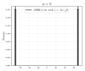
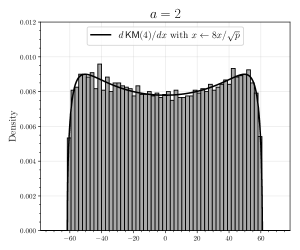
Refer to captionRefer to captionRefer to caption
Figure 1: Spectra of localizations. We plot the spectrum of 𝑨Gp,Isubscript𝑨subscript𝐺𝑝𝐼\bm{A}_{G_{p,I}} (with the Perron-Frobenius largest eigenvalue omitted) along with the density of 𝖪𝖬(2a)𝖪𝖬superscript2𝑎\mathsf{KM}(2^{a}) suitably rescaled, for p=20,021𝑝20021p=$20,021$ and one choice of I𝐼I for each size a=|I|{0,1,2,3,4,5}𝑎𝐼012345a=|I|\in\{0,1,2,3,4,5\}.
Refer to caption
Refer to caption
Refer to caption
Figure 2: Distributional distance of e.s.d. of localizations to Kesten-McKay. We plot the Kolmogorov distance between the empirical spectral distribution of 2a+1p𝑨Gp,Isuperscript2𝑎1𝑝subscript𝑨subscript𝐺𝑝𝐼\frac{2^{a+1}}{\sqrt{p}}\bm{A}_{G_{p,I}} and 𝖪𝖬(2a)𝖪𝖬superscript2𝑎\mathsf{KM}(2^{a}) for a{1,2,3}𝑎123a\in\{1,2,3\} and all p5000𝑝5000p\leq$5000$. For a=1𝑎1a=1 (respectively a=2𝑎2a=2) all Gp,Isubscript𝐺𝑝𝐼G_{p,I} are isomorphic to Gp,{0}subscript𝐺𝑝0G_{p,\{0\}} (respectively Gp,{0,g}subscript𝐺𝑝0𝑔G_{p,\{0,g\}} for g𝑔g a generator of 𝔽p×superscriptsubscript𝔽𝑝\mathbb{F}_{p}^{\times}), so we plot one value. For a=3𝑎3a=3, all Gp,Isubscript𝐺𝑝𝐼G_{p,I} are isomorphic to Gp,{0,g,x}subscript𝐺𝑝0𝑔𝑥G_{p,\{0,g,x\}} for some x𝑥x, so we plot the mean, minimum, and maximum of the Kolmogorov distance over all x𝑥x with {0,g,x}3(Gp)0𝑔𝑥subscript3subscript𝐺𝑝\{0,g,x\}\in\mathcal{I}_{3}(G_{p}).
Refer to caption
Refer to caption
Refer to caption
Figure 3: Minimum eigenvalues of localizations. We plot λmin(𝑨Gp,I)subscript𝜆subscript𝑨subscript𝐺𝑝𝐼-\lambda_{\min}(\bm{A}_{G_{p,I}}) over all Ia(Gp)𝐼subscript𝑎subscript𝐺𝑝I\in\mathcal{I}_{a}(G_{p}) for p5000𝑝5000p\leq$5000$ and a{1,2,3}𝑎123a\in\{1,2,3\}, along with the corresponding prediction from Conjecture 1.9. The remarks from Figure 2 concerning the distinction between a{1,2}𝑎12a\in\{1,2\} and a=3𝑎3a=3 apply here as well.

References

  • [Bas65] Leonid Alexandrovich Bassalygo. New upper bounds for error correcting codes. Problemy Peredachi Informatsii, 1(4):41–44, 1965.
  • [Ber68] ER Berlekamp. Algebraic coding theory. New York, 8, 1968.
  • [BFMW13] Afonso S Bandeira, Matthew Fickus, Dustin G Mixon, and Percy Wong. The road to deterministic matrices with the restricted isometry property. Journal of Fourier Analysis and Applications, 19(6):1123–1149, 2013.
  • [Bha13] Rajendra Bhatia. Matrix analysis, volume 169. Springer Science & Business Media, 2013.
  • [BHK+19] Boaz Barak, Samuel Hopkins, Jonathan Kelner, Pravesh K Kothari, Ankur Moitra, and Aaron Potechin. A nearly tight sum-of-squares lower bound for the planted clique problem. SIAM Journal on Computing, 48(2):687–735, 2019.
  • [BMM17] Afonso S Bandeira, Dustin G Mixon, and Joel Moreira. A conditional construction of restricted isometries. International Mathematics Research Notices, 2017(2):372–381, 2017.
  • [BMR13] Christine Bachoc, Máté Matolcsi, and Imre Z Ruzsa. Squares and difference sets in finite fields. Integers, 13:A77, 2013.
  • [BT19] Jess Banks and Luca Trevisan. Vector colorings of random, Ramanujan, and large-girth irregular graphs. arXiv preprint arXiv:1907.02539, 2019.
  • [BV08] Christine Bachoc and Frank Vallentin. New upper bounds for kissing numbers from semidefinite programming. Journal of the American Mathematical Society, 21(3):909–924, 2008.
  • [CE03] Henry Cohn and Noam Elkies. New upper bounds on sphere packings I. Annals of Mathematics, pages 689–714, 2003.
  • [CGMS23] Marcelo Campos, Simon Griffiths, Robert Morris, and Julian Sahasrabudhe. An exponential improvement for diagonal Ramsey. arXiv preprint arXiv:2303.09521, 2023.
  • [CGW89] Fan R. K. Chung, Ronald L. Graham, and Richard M. Wilson. Quasi-random graphs. Combinatorica, 9:345–362, 1989.
  • [Chu89] Fan RK Chung. Diameters and eigenvalues. Journal of the American Mathematical Society, 2(2):187–196, 1989.
  • [CI00] J Brian Conrey and Henryk Iwaniec. The cubic moment of central values of automorphic L𝐿L-functions. Annals of Mathematics, 151(3):1175–1216, 2000.
  • [Coh16] Gil Cohen. Two-source dispersers for polylogarithmic entropy and improved Ramsey graphs. In 48th Annual ACM Symposium on Theory of Computing (STOC 2016), pages 278–284, 2016.
  • [CVVE12] Jiahao Chen, Troy Van Voorhis, and Alan Edelman. Partial freeness of random matrices. arXiv preprint arXiv:1204.2257, 2012.
  • [CZ16] Eshan Chattopadhyay and David Zuckerman. Explicit two-source extractors and resilient functions. In 48th Annual ACM Symposium on Theory of Computing (STOC 2016), pages 670–683, 2016.
  • [DBSW21] Daniel Di Benedetto, József Solymosi, and Ethan P White. On the directions determined by a Cartesian product in an affine Galois plane. Combinatorica, 41(6):755–763, 2021.
  • [Del72] Philippe Delsarte. Bounds for unrestricted codes, by linear programming. Philips Res. Rep, 27:272–289, 1972.
  • [Del73] Philippe Delsarte. An algebraic approach to the association schemes of coding theory. Philips Res. Rep. Suppl., 10:vi–97, 1973.
  • [DGIV77] P Deligne, A Grothendieck, L Illusie, and JL Verdier. Séminaire de géométrie algébrique du Bois Marie – Cohomologie étale – (SGA 4 1/2). 1977.
  • [dLV15] David de Laat and Frank Vallentin. A semidefinite programming hierarchy for packing problems in discrete geometry. Mathematical Programming, 151(2):529–553, 2015.
  • [DM15] Yash Deshpande and Andrea Montanari. Improved sum-of-squares lower bounds for hidden clique and hidden submatrix problems. In 28th Annual Conference on Learning Theory (COLT 2015), pages 523–562, 2015.
  • [Erd47] Paul Erdös. Some remarks on the theory of graphs. 1947.
  • [ES35] Paul Erdös and George Szekeres. A combinatorial problem in geometry. Compositio Mathematica, 2:463–470, 1935.
  • [GLV09] Nebojša Gvozdenović, Monique Laurent, and Frank Vallentin. Block-diagonal semidefinite programming hierarchies for 0/1 programming. Operations Research Letters, 37(1):27–31, 2009.
  • [GN08] Chris D Godsil and Michael W Newman. Eigenvalue bounds for independent sets. Journal of Combinatorial Theory, Series B, 98(4):721–734, 2008.
  • [GR90] Sidney West Graham and CJ Ringrose. Lower bounds for least quadratic non-residues. In Analytic number theory, pages 269–309. Springer, 1990.
  • [GR01] Chris D Godsil and Gordon Royle. Algebraic graph theory, volume 207 of Graduate Texts in Mathematics. Springer-Verlag, 2001.
  • [GS02] Alison L Gibbs and Francis Edward Su. On choosing and bounding probability metrics. International Statistical Review, 70(3):419–435, 2002.
  • [Hae78] Willem Haemers. An upper bound for the Shannon capacity of a graph. In Colloq. Math. Soc. János Bolyai, volume 25, pages 267–272. Hungary, 1978.
  • [Hae95] Willem H Haemers. Interlacing eigenvalues and graphs. Linear Algebra and its Applications, 226:593–616, 1995.
  • [Hae21] Willem H Haemers. Hoffman’s ratio bound. Linear Algebra and its Applications, 617:215–219, 2021.
  • [HKP+18] Samuel B Hopkins, Pravesh Kothari, Aaron Henry Potechin, Prasad Raghavendra, and Tselil Schramm. On the integrality gap of degree-4 sum of squares for planted clique. ACM Transactions on Algorithms (TALG), 14(3):1–31, 2018.
  • [Hof70] Alan J Hoffman. On eigenvalues and colorings of graphs. In Bernard Harris, editor, Graph theory and its applications. 1970.
  • [HP21] Brandon Hanson and Giorgis Petridis. Refined estimates concerning sumsets contained in the roots of unity. Proceedings of the London Mathematical Society, 122(3):353–358, 2021.
  • [HZG17] Marina Haikin, Ram Zamir, and Matan Gavish. Random subsets of structured deterministic frames have MANOVA spectra. Proceedings of the National Academy of Sciences, 114(26):E5024–E5033, 2017.
  • [IK21] Henryk Iwaniec and Emmanuel Kowalski. Analytic number theory, volume 53. American Mathematical Soc., 2021.
  • [IR90] Kenneth Ireland and Michael Ira Rosen. A classical introduction to modern number theory, volume 84. Springer Science & Business Media, 1990.
  • [Kat88] Nicholas M Katz. Gauss sums, Kloosterman sums, and monodromy groups. Number 116. Princeton University Press, 1988.
  • [Kat99] Nicholas M Katz. Estimates for “singular” exponential sums. International Mathematics Research Notices, 1999(16):875–899, 1999.
  • [Kat07] Nicholas M. Katz. Estimates for nonsingular mixed character sums. International Mathematics Research Notices, 01 2007.
  • [Kat08] Nicholas M Katz. Estimates for mixed character sums. Geom. Funct. Anal, 18(4):1251–1269, 2008.
  • [Kel10] Dubi Kelmer. Distribution of twisted Kloosterman sums modulo prime powers. International Journal of Number Theory, 6(02):271–280, 2010.
  • [KL95] Gil Kalai and Nathan Linial. On the distance distribution of codes. IEEE Transactions on Information Theory, 41(5):1467–1472, 1995.
  • [Knu93] Donald E Knuth. The sandwich theorem. arXiv preprint math/9312214, 1993.
  • [Kun23] Dmitriy Kunisky. Generic MANOVA limit theorems for products of projections. arXiv preprint arXiv:2301.09543, 2023.
  • [KY22] Dmitriy Kunisky and Xifan Yu. A degree 4 sum-of-squares lower bound for the clique number of the Paley graph. arXiv preprint arXiv:2211.02713, 2022.
  • [KZ96] Nicholas M Katz and Zhiyong Zheng. On the uniform distribution of Gauss sums and Jacobi sums. Progress in Mathematics, 139:537–558, 1996.
  • [Las01] Jean B Lasserre. Global optimization with polynomials and the problem of moments. SIAM Journal on Optimization, 11(3):796–817, 2001.
  • [Lau03] Monique Laurent. A comparison of the Sherali-Adams, Lovász-Schrijver, and Lasserre relaxations for 0–1 programming. Mathematics of Operations Research, 28(3):470–496, 2003.
  • [Liu02] Chunlei Liu. Twisted higher moments of Kloosterman sums. Proceedings of the American Mathematical Society, 130(7):1887–1892, 2002.
  • [Lov79] László Lovász. On the Shannon capacity of a graph. IEEE Transactions on Information Theory, 25(1):1–7, 1979.
  • [Lov03] László Lovász. Semidefinite programs and combinatorial optimization. In Recent advances in algorithms and combinatorics, pages 137–194. Springer, 2003.
  • [LZZ18] Qing Lu, Weizhe Zheng, and Zhiyong Zheng. On the distribution of Jacobi sums. Journal für die reine und angewandte Mathematik (Crelles Journal), 2018(741):67–86, 2018.
  • [MMP19] Mark Magsino, Dustin G Mixon, and Hans Parshall. Linear programming bounds for cliques in Paley graphs. In Wavelets and Sparsity XVIII, volume 11138, page 111381H. International Society for Optics and Photonics, 2019.
  • [MMP21] Mark Magsino, Dustin G Mixon, and Hans Parshall. Kesten–McKay law for random subensembles of Paley equiangular tight frames. Constructive Approximation, 53:381–402, 2021.
  • [Mon71] Hugh L Montgomery. Topics in multiplicative number theory, volume 227. Springer, 1971.
  • [MP06] E Maistrelli and DB Penman. Some colouring problems for Paley graphs. Discrete Mathematics, (306):99–106, 2006.
  • [MPW15] Raghu Meka, Aaron Potechin, and Avi Wigderson. Sum-of-squares lower bounds for planted clique. In 47th Annual ACM Symposium on Theory of Computing (STOC 2015), pages 87–96. ACM, 2015.
  • [Mra17] Rudi Mrazović. A random model for the Paley graph. The Quarterly Journal of Mathematics, 68(1):193–206, 2017.
  • [MS17] James A Mingo and Roland Speicher. Free probability and random matrices, volume 35. Springer, 2017.
  • [MW13] Raghu Meka and Avi Wigderson. Association schemes, non-commutative polynomial concentration, and sum-of-squares lower bounds for planted clique. In Electronic Colloquium on Computational Complexity (ECCC), volume 20, page 10, 2013.
  • [NS06] Alexandru Nica and Roland Speicher. Lectures on the combinatorics of free probability, volume 13. Cambridge University Press, 2006.
  • [Pan21] Shuo Pang. SOS lower bound for exact planted clique. In 36th Computational Complexity Conference (CCC 2021). Schloss Dagstuhl-Leibniz-Zentrum für Informatik, 2021.
  • [Par03] Pablo A Parrilo. Semidefinite programming relaxations for semialgebraic problems. Mathematical Programming, 96(2):293–320, 2003.
  • [Ram29] Frank P Ramsey. On a problem of formal logic. Proceedings of the London Mathematical Society, (30):264–286, 1929.
  • [RL05] Antonio Rojas-León. Estimates for singular multiplicative character sums. International Mathematics Research Notices, 2005(20):1221–1234, 2005.
  • [RL22] Antonio Rojas-León. On a generalization of Jacobi sums. Finite Fields and Their Applications, 77:101944, 2022.
  • [RS15] Prasad Raghavendra and Tselil Schramm. Tight lower bounds for planted clique in the degree-4 SOS program. arXiv preprint arXiv:1507.05136, 2015.
  • [SA90] Hanif D Sherali and Warren P Adams. A hierarchy of relaxations between the continuous and convex hull representations for zero-one programming problems. SIAM Journal on Discrete Mathematics, 3(3):411–430, 1990.
  • [Sch79] Alexander Schrijver. A comparison of the Delsarte and Lovász bounds. IEEE Transactions on Information Theory, 25(4):425–429, 1979.
  • [Sch05] Alexander Schrijver. New code upper bounds from the Terwilliger algebra and semidefinite programming. IEEE Transactions on Information Theory, 51(8):2859–2866, 2005.
  • [She86] James B Shearer. Lower bounds for small diagonal Ramsey numbers. Journal of Combinatorial Theory, Series A, 42(2):302–304, 1986.
  • [Sin18] John Sinkovic. A graph for which the inertia bound is not tight. Journal of Algebraic Combinatorics, 47(1):39–50, 2018.
  • [Spe94] Joel Spencer. Ten lectures on the probabilistic method. SIAM, 1994.
  • [ST18] Ilya Soloveychik and Vahid Tarokh. Asymptotically pseudo-independent matrices. arXiv preprint arXiv:1809.00408, 2018.
  • [SXT17] Ilya Soloveychik, Yu Xiang, and Vahid Tarokh. Pseudo-Wigner matrices. IEEE Transactions on Information Theory, 64(4):3170–3178, 2017.
  • [SXT18] Ilya Soloveychik, Yu Xiang, and Vahid Tarokh. Symmetric pseudo-random matrices. IEEE Transactions on Information Theory, 64(4):3179–3196, 2018.
  • [Vad12] Salil P Vadhan. Pseudorandomness. Foundations and Trends® in Theoretical Computer Science, 7(1–3):1–336, 2012.
  • [VDN92] Dan V Voiculescu, Ken J Dykema, and Alexandru Nica. Free random variables. Number 1. American Mathematical Society, 1992.
  • [Wac80] Kenneth W Wachter. The limiting empirical measure of multiple discriminant ratios. The Annals of Statistics, pages 937–957, 1980.
  • [Wig19] Avi Wigderson. Mathematics and computation: A theory revolutionizing technology and science. Princeton University Press, 2019.
  • [Xi18] Ping Xi. Equidistributions of Jacobi sums. arXiv preprint arXiv:1809.04286, 2018.
  • [Xi22] Ping Xi. Moments and equidistributions of multiplicative analogues of Kloosterman sums. Acta Arithmetica, (206):245–275, 2022.
  • [Yip22] Chi Hoi Yip. On the clique number of Paley graphs of prime power order. Finite Fields and Their Applications, 77:101930, 2022.

Appendix A Lovász ϑitalic-ϑ\vartheta function on degree 2 localization

Refer to caption
Figure 4: Bound from Lovász ϑitalic-ϑ\vartheta function on 2-localization. We plot the bound on α(Gp)𝛼subscript𝐺𝑝\alpha(G_{p}) from (104) together with the “trivial” p𝑝\sqrt{p} bound and the Hanson-Petridis bound of Theorem 1.2 for all p800𝑝800p\leq 800.

We explore empirically a simple ad hoc improvement of the proof strategy pursued by [MMP19]. Recall that their approach applied the Lovász ϑitalic-ϑ\vartheta function (equivalently, the degree 2 SOS relaxation) together with degree 1 localization, using the bound

α(Gp)1+maxI1(Gp)ϑ(Gp,I)=1+ϑ(Gp,{0}),𝛼subscript𝐺𝑝1subscript𝐼subscript1subscript𝐺𝑝italic-ϑsubscript𝐺𝑝𝐼1italic-ϑsubscript𝐺𝑝0\alpha(G_{p})\leq 1+\max_{I\in\mathcal{I}_{1}(G_{p})}\vartheta(G_{p,I})=1+\vartheta(G_{p,\{0\}}), (103)

where we have used that, by Corollary 3.2, all of the Gp,{x}subscript𝐺𝑝𝑥G_{p,\{x\}} are isomorphic. They found empirically that the right-hand side is very close to the Hanson-Petridis bound of Theorem 1.2. These empirical experiments were eased by the observation that Gp,{0}subscript𝐺𝑝0G_{p,\{0\}} has a circulant adjacency matrix (see the discussion in Section 5.1), whereby ϑ(Gp,{0})italic-ϑsubscript𝐺𝑝0\vartheta(G_{p,\{0\}}) may be reduced to a linear rather than semidefinite program.

Consider the same approach with degree 2 localization. Let g𝑔g be a multiplicative generator of 𝔽p×superscriptsubscript𝔽𝑝\mathbb{F}_{p}^{\times}. We have

α(Gp)2+maxI2(Gp)ϑ(Gp,I)=2+ϑ(Gp,{0,g}),𝛼subscript𝐺𝑝2subscript𝐼subscript2subscript𝐺𝑝italic-ϑsubscript𝐺𝑝𝐼2italic-ϑsubscript𝐺𝑝0𝑔\alpha(G_{p})\leq 2+\max_{I\in\mathcal{I}_{2}(G_{p})}\vartheta(G_{p,I})=2+\vartheta(G_{p,\{0,g\}}), (104)

where again we have that, by Corollary 3.2, all of the Gp,Isubscript𝐺𝑝𝐼G_{p,I} for I2(Gp)𝐼subscript2subscript𝐺𝑝I\in\mathcal{I}_{2}(G_{p}) are isomorphic. Unfortunately, the adjacency matrix of Gp,{0,g}subscript𝐺𝑝0𝑔G_{p,\{0,g\}} is not circulant, so there is not enough symmetry remaining in this problem to reduce ϑ(Gp,{0,g})italic-ϑsubscript𝐺𝑝0𝑔\vartheta(G_{p,\{0,g\}}) to a linear program. Still, unlike higher-degree localization bounds, this bound only calls for solving one semidefinite program for a given value of p𝑝p, and so is relatively computationally tractable. We compare this bound to the trivial and Hanson-Petridis bounds in Figure 4, and find that it appears to improve further on the constant in front of p𝑝\sqrt{p}. We state this formally below.

Conjecture A.1 (Improving on Hanson-Petridis).

For some ε>0𝜀0\varepsilon>0 and for all sufficiently large p𝑝p, ϑ(Gp,{0,g})(12ε)pitalic-ϑsubscript𝐺𝑝0𝑔12𝜀𝑝\vartheta(G_{p,\{0,g\}})\leq(\frac{1}{\sqrt{2}}-\varepsilon)\sqrt{p}.

The natural approach to Conjecture A.1 is to build a feasible point for SDP dual to ϑ(Gp,{0,g})italic-ϑsubscript𝐺𝑝0𝑔\vartheta(G_{p,\{0,g\}}). We have not succeeded in finding a construction that is tractable to analyze theoretically. The main difficulty seems to be precisely the lower amount of symmetry (or higher amount of pseudorandomness) in Gp,{0,g}subscript𝐺𝑝0𝑔G_{p,\{0,g\}} compared to Gpsubscript𝐺𝑝G_{p} and Gp,{0}subscript𝐺𝑝0G_{p,\{0\}}; numerically, the dual variables at optimality do not seem to exhibit any particularly simple structure that we can easily exploit.

Appendix B Towards higher-degree estimates

B.1 One special degree 2 estimate

We give one example of a degree 2 necklace character sum that actually reduces to the degree 1 necklace character sums treated in Theorem 1.18. Unfortunately, this seems to be a special phenomenon thanks to the symmetry of this sum, which we do not expect to apply more generally.

Theorem B.1.

For any distinct z,z𝔽p𝑧superscript𝑧subscript𝔽𝑝z,z^{\prime}\in\mathbb{F}_{p},

|Σ({z,z},,{z,z})|kp(k+1)/2+2kpk/2=Ok(p(k+1)/2).Σ𝑧superscript𝑧𝑧superscript𝑧𝑘superscript𝑝𝑘12superscript2𝑘superscript𝑝𝑘2subscript𝑂𝑘superscript𝑝𝑘12|\Sigma(\{z,z^{\prime}\},\dots,\{z,z^{\prime}\})|\leq kp^{(k+1)/2}+2^{k}p^{k/2}=O_{k}(p^{(k+1)/2}). (105)
Proof.

Let us write Σ\colonequalsΣ({z,z},,{z,z})Σ\colonequalsΣ𝑧superscript𝑧𝑧superscript𝑧\Sigma\colonequals\Sigma(\{z,z^{\prime}\},\dots,\{z,z^{\prime}\}). By changing variables xixi+zsubscript𝑥𝑖subscript𝑥𝑖superscript𝑧x_{i}\leftarrow x_{i}+z^{\prime} in ΣΣ\Sigma, we may assume without loss of generality that z=0superscript𝑧0z^{\prime}=0 (and thus z0𝑧0z\neq 0). We then have

ΣΣ\displaystyle\Sigma =x1,,xk𝔽pχ(x1(x1z)(x1x2)xk(xkz)(xkx1))absentsubscriptsubscript𝑥1subscript𝑥𝑘subscript𝔽𝑝𝜒subscript𝑥1subscript𝑥1𝑧subscript𝑥1subscript𝑥2subscript𝑥𝑘subscript𝑥𝑘𝑧subscript𝑥𝑘subscript𝑥1\displaystyle=\sum_{x_{1},\dots,x_{k}\in\mathbb{F}_{p}}\chi\big{(}x_{1}(x_{1}-z)(x_{1}-x_{2})\cdots x_{k}(x_{k}-z)(x_{k}-x_{1})\big{)}
=x1,,xk𝔽p×χ(x1(x1z)(x1x2)xk(xkz)(xkx1))absentsubscriptsubscript𝑥1subscript𝑥𝑘superscriptsubscript𝔽𝑝𝜒subscript𝑥1subscript𝑥1𝑧subscript𝑥1subscript𝑥2subscript𝑥𝑘subscript𝑥𝑘𝑧subscript𝑥𝑘subscript𝑥1\displaystyle=\sum_{x_{1},\dots,x_{k}\in\mathbb{F}_{p}^{\times}}\chi\big{(}x_{1}(x_{1}-z)(x_{1}-x_{2})\cdots x_{k}(x_{k}-z)(x_{k}-x_{1})\big{)}
=x1,,xk𝔽p×χ((1zx11)(x11x21)(1zxk1)(xk1x11))absentsubscriptsubscript𝑥1subscript𝑥𝑘superscriptsubscript𝔽𝑝𝜒1𝑧superscriptsubscript𝑥11superscriptsubscript𝑥11superscriptsubscript𝑥211𝑧superscriptsubscript𝑥𝑘1superscriptsubscript𝑥𝑘1superscriptsubscript𝑥11\displaystyle=\sum_{x_{1},\dots,x_{k}\in\mathbb{F}_{p}^{\times}}\chi\big{(}(1-zx_{1}^{-1})(x_{1}^{-1}-x_{2}^{-1})\cdots(1-zx_{k}^{-1})(x_{k}^{-1}-x_{1}^{-1})\big{)}
=χ(z)kx1,,xk𝔽p×χ((z1x1)(x1x2)(z1xk)(xkx1))absent𝜒superscript𝑧𝑘subscriptsubscript𝑥1subscript𝑥𝑘superscriptsubscript𝔽𝑝𝜒superscript𝑧1subscript𝑥1subscript𝑥1subscript𝑥2superscript𝑧1subscript𝑥𝑘subscript𝑥𝑘subscript𝑥1\displaystyle=\chi(z)^{k}\sum_{x_{1},\dots,x_{k}\in\mathbb{F}_{p}^{\times}}\chi\big{(}(z^{-1}-x_{1})(x_{1}-x_{2})\cdots(z^{-1}-x_{k})(x_{k}-x_{1})\big{)} (106)

This sum only differs by the restriction to 𝔽p×superscriptsubscript𝔽𝑝\mathbb{F}_{p}^{\times} from the degree 1 necklace character sum

Σ({z1},,{z1})Σsuperscript𝑧1superscript𝑧1\displaystyle\Sigma(\{z^{-1}\},\dots,\{z^{-1}\}) =x1,,xk𝔽pχ((z1x1)(x1x2)(z1xk)(xkx1))absentsubscriptsubscript𝑥1subscript𝑥𝑘subscript𝔽𝑝𝜒superscript𝑧1subscript𝑥1subscript𝑥1subscript𝑥2superscript𝑧1subscript𝑥𝑘subscript𝑥𝑘subscript𝑥1\displaystyle=\sum_{x_{1},\dots,x_{k}\in\mathbb{F}_{p}}\chi\big{(}(z^{-1}-x_{1})(x_{1}-x_{2})\cdots(z^{-1}-x_{k})(x_{k}-x_{1})\big{)}
and our plan will be to bound the difference between these two. To that end, we view the above in linear-algebraic terms as
=Tr(𝑫𝑺)k,\displaystyle=\operatorname{Tr}(\bm{D}\bm{S})^{k}, (107)

where 𝑫𝔽p×𝔽p𝑫superscriptsubscript𝔽𝑝subscript𝔽𝑝\bm{D}\in\mathbb{R}^{\mathbb{F}_{p}\times\mathbb{F}_{p}} is the diagonal matrix with diagonal entries Dxx=χ(z1x)subscript𝐷𝑥𝑥𝜒superscript𝑧1𝑥D_{xx}=\chi(z^{-1}-x) and 𝑺𝑺\bm{S} is the {±1}plus-or-minus1\{\pm 1\}-valued adjacency matrix of Gpsubscript𝐺𝑝G_{p}. Let 𝑫~~𝑫\widetilde{\bm{D}} be 𝑫𝑫\bm{D} with the row and column indexed by 0𝔽p0subscript𝔽𝑝0\in\mathbb{F}_{p} set to zero. Then, we have

𝑫=χ(z)𝒆0𝒆0+𝑫~.𝑫𝜒𝑧subscript𝒆0superscriptsubscript𝒆0top~𝑫\bm{D}=\chi(z)\bm{e}_{0}\bm{e}_{0}^{\top}+\widetilde{\bm{D}}. (108)

Note that the sum we were originally interested in is

Σ=χ(z)kTr(𝑫~𝑺)k.\Sigma=\chi(z)^{k}\operatorname{Tr}(\widetilde{\bm{D}}\bm{S})^{k}. (109)

As in our arguments in Section 4, let us define

𝑯0subscript𝑯0\displaystyle\bm{H}_{0} \colonequalsχ(z)𝒆0𝒆0,\colonequals𝜒𝑧subscript𝒆0superscriptsubscript𝒆0top\displaystyle\colonequals\chi(z)\bm{e}_{0}\bm{e}_{0}^{\top}, (110)
𝑯1subscript𝑯1\displaystyle\bm{H}_{1} \colonequals𝑫~.\colonequals~𝑫\displaystyle\colonequals\widetilde{\bm{D}}. (111)

Then, we have

Σ({z1},,{z1})=χ(z)kΣ+s1,,sk{0,1}some si=0Tr(𝑯s1𝑯sk).Σsuperscript𝑧1superscript𝑧1𝜒superscript𝑧𝑘Σsubscriptsubscript𝑠1subscript𝑠𝑘01some subscript𝑠𝑖0Trsubscript𝑯subscript𝑠1subscript𝑯subscript𝑠𝑘\Sigma(\{z^{-1}\},\dots,\{z^{-1}\})=\chi(z)^{k}\Sigma+\sum_{\begin{subarray}{c}s_{1},\dots,s_{k}\in\{0,1\}\\ \text{some }s_{i}=0\end{subarray}}\operatorname{Tr}(\bm{H}_{s_{1}}\cdots\bm{H}_{s_{k}}). (112)

Rearranging, we have

|Σ|Σ\displaystyle|\Sigma| |Σ({z1},,{z1})|+s1,,sk{0,1}some si=0|Tr(𝑯s1𝑺𝑯sk𝑺)|absentΣsuperscript𝑧1superscript𝑧1subscriptsubscript𝑠1subscript𝑠𝑘01some subscript𝑠𝑖0Trsubscript𝑯subscript𝑠1𝑺subscript𝑯subscript𝑠𝑘𝑺\displaystyle\leq|\Sigma(\{z^{-1}\},\dots,\{z^{-1}\})|+\sum_{\begin{subarray}{c}s_{1},\dots,s_{k}\in\{0,1\}\\ \text{some }s_{i}=0\end{subarray}}|\operatorname{Tr}(\bm{H}_{s_{1}}\bm{S}\cdots\bm{H}_{s_{k}}\bm{S})|
Here, the first quantity is bounded by Theorem 1.18. Each term in the second sum may be written |𝒆0𝑯𝒆0|𝑯superscriptsubscript𝒆0top𝑯subscript𝒆0norm𝑯|\bm{e}_{0}^{\top}\bm{H}\bm{e}_{0}|\leq\|\bm{H}\| for some 𝑯𝑯\bm{H} with 𝑯𝑺kpk/2norm𝑯superscriptnorm𝑺𝑘superscript𝑝𝑘2\|\bm{H}\|\leq\|\bm{S}\|^{k}\leq p^{k/2}. Thus, we find
kp(k+1)/2+2kpk/2,absent𝑘superscript𝑝𝑘12superscript2𝑘superscript𝑝𝑘2\displaystyle\leq kp^{(k+1)/2}+2^{k}p^{k/2}, (113)

where we have substituted in the explicit bound (85) from our proof of Theorem 1.18, completing the proof. ∎

B.2 General reduction to Gauss sum polynomials

We mention one approach that might prove fruitful for the general case of Conjecture 1.14, which generalizes our first approach to the proof of Theorem 1.18. We will show that we can rewrite a general necklace character sum as a large polynomial in Jacobi sums, and therefore in angles of Gauss sums.

The following standard result expresses that the Jacobi sums are the multiplicative Fourier transform of additive translation of a multiplicative character.

Proposition B.2.

For all x𝔽p×𝑥superscriptsubscript𝔽𝑝x\in\mathbb{F}_{p}^{\times},

ϕ(1x)=1p1ψ𝔽p×^J(ϕ,ψ)ψ¯(x).italic-ϕ1𝑥1𝑝1subscript𝜓^superscriptsubscript𝔽𝑝𝐽italic-ϕ𝜓¯𝜓𝑥\phi(1-x)=\frac{1}{p-1}\sum_{\psi\in\widehat{\mathbb{F}_{p}^{\times}}}J(\phi,\psi)\overline{\psi}(x). (114)

Suppose we are interested in controlling a general necklace character sum

Σ(Z1,,Zk)=x1,,xk𝔽pχ(x2x1)χ(xkxk1)χ(x1xk)i=1kzZiχ(xiz).Σsubscript𝑍1subscript𝑍𝑘subscriptsubscript𝑥1subscript𝑥𝑘subscript𝔽𝑝𝜒subscript𝑥2subscript𝑥1𝜒subscript𝑥𝑘subscript𝑥𝑘1𝜒subscript𝑥1subscript𝑥𝑘superscriptsubscriptproduct𝑖1𝑘subscriptproduct𝑧subscript𝑍𝑖𝜒subscript𝑥𝑖𝑧\Sigma(Z_{1},\dots,Z_{k})=\sum_{x_{1},\dots,x_{k}\in\mathbb{F}_{p}}\chi(x_{2}-x_{1})\cdots\chi(x_{k}-x_{k-1})\chi(x_{1}-x_{k})\prod_{i=1}^{k}\prod_{z\in Z_{i}}\chi(x_{i}-z). (115)

For constant degree a𝑎a, since |Z1Zk|asubscript𝑍1subscript𝑍𝑘𝑎|Z_{1}\cup\cdots\cup Z_{k}|\leq a, by a suitable change of variables we may assume without loss of generality that 0Zi0subscript𝑍𝑖0\notin Z_{i} for all i𝑖i. By the argument from Theorem B.1, it also suffices to control the restriction to xi𝔽p×subscript𝑥𝑖superscriptsubscript𝔽𝑝x_{i}\in\mathbb{F}_{p}^{\times}, so we will look at the quantity

Σ~\colonequalsx1,,xk𝔽p×χ(x2x1)χ(xkxk1)χ(x1xk)i=1kzZiχ(xiz).~Σ\colonequalssubscriptsubscript𝑥1subscript𝑥𝑘superscriptsubscript𝔽𝑝𝜒subscript𝑥2subscript𝑥1𝜒subscript𝑥𝑘subscript𝑥𝑘1𝜒subscript𝑥1subscript𝑥𝑘superscriptsubscriptproduct𝑖1𝑘subscriptproduct𝑧subscript𝑍𝑖𝜒subscript𝑥𝑖𝑧\widetilde{\Sigma}\colonequals\sum_{x_{1},\dots,x_{k}\in\mathbb{F}_{p}^{\times}}\chi(x_{2}-x_{1})\cdots\chi(x_{k}-x_{k-1})\chi(x_{1}-x_{k})\prod_{i=1}^{k}\prod_{z\in Z_{i}}\chi(x_{i}-z). (116)

Let us define zijsubscript𝑧𝑖𝑗z_{ij} such that Zi={zi1,,zimi}subscript𝑍𝑖subscript𝑧𝑖1subscript𝑧𝑖subscript𝑚𝑖Z_{i}=\{z_{i1},\dots,z_{im_{i}}\} for mi=|Zi|subscript𝑚𝑖subscript𝑍𝑖m_{i}=|Z_{i}|. We will reserve the indices i,j𝑖𝑗i,j for enumerating these variables below. We also assume all index arithmetic is performed modulo k𝑘k. We apply Proposition B.2 first to each of the χ(xbz)𝜒subscript𝑥𝑏𝑧\chi(x_{b}-z) terms and then to each of the χ(xbxb1)𝜒subscript𝑥𝑏subscript𝑥𝑏1\chi(x_{b}-x_{b-1}), obtaining

Σ~~Σ\displaystyle\widetilde{\Sigma} =i,jχ(zij)1(p1)i=1kmiψij𝔽p×^x1,,xk𝔽p×b=1kχ(xbxb1)i,jJ(χ,ψij)ψij¯(zij1xi)absentsubscriptproduct𝑖𝑗𝜒subscript𝑧𝑖𝑗1superscript𝑝1superscriptsubscript𝑖1𝑘subscript𝑚𝑖subscriptsubscript𝜓𝑖𝑗^superscriptsubscript𝔽𝑝subscriptsubscript𝑥1subscript𝑥𝑘superscriptsubscript𝔽𝑝superscriptsubscriptproduct𝑏1𝑘𝜒subscript𝑥𝑏subscript𝑥𝑏1subscriptproduct𝑖𝑗𝐽𝜒subscript𝜓𝑖𝑗¯subscript𝜓𝑖𝑗superscriptsubscript𝑧𝑖𝑗1subscript𝑥𝑖\displaystyle=\prod_{i,j}\chi(z_{ij})\frac{1}{(p-1)^{\sum_{i=1}^{k}m_{i}}}\sum_{\psi_{ij}\in\widehat{\mathbb{F}_{p}^{\times}}}\sum_{x_{1},\dots,x_{k}\in\mathbb{F}_{p}^{\times}}\prod_{b=1}^{k}\chi(x_{b}-x_{b-1})\prod_{i,j}J(\chi,\psi_{ij})\overline{\psi_{ij}}(z_{ij}^{-1}x_{i})
=i,jχ(zij)1(p1)k+miψij𝔽p×^ϕ1,,ϕk𝔽p×^x1,,xk𝔽p×absentsubscriptproduct𝑖𝑗𝜒subscript𝑧𝑖𝑗1superscript𝑝1𝑘subscript𝑚𝑖subscriptsubscript𝜓𝑖𝑗^superscriptsubscript𝔽𝑝subscriptsubscriptitalic-ϕ1subscriptitalic-ϕ𝑘^superscriptsubscript𝔽𝑝subscriptsubscript𝑥1subscript𝑥𝑘superscriptsubscript𝔽𝑝\displaystyle=\prod_{i,j}\chi(z_{ij})\frac{1}{(p-1)^{k+\sum m_{i}}}\sum_{\psi_{ij}\in\widehat{\mathbb{F}_{p}^{\times}}}\sum_{\phi_{1},\dots,\phi_{k}\in\widehat{\mathbb{F}_{p}^{\times}}}\sum_{x_{1},\dots,x_{k}\in\mathbb{F}_{p}^{\times}}
b=1kϕb¯(xbxb11)χ(xb)J(χ,ϕb)i,jJ(χ,ψij)ψij¯(zij1xi)superscriptsubscriptproduct𝑏1𝑘¯subscriptitalic-ϕ𝑏subscript𝑥𝑏superscriptsubscript𝑥𝑏11𝜒subscript𝑥𝑏𝐽𝜒subscriptitalic-ϕ𝑏subscriptproduct𝑖𝑗𝐽𝜒subscript𝜓𝑖𝑗¯subscript𝜓𝑖𝑗superscriptsubscript𝑧𝑖𝑗1subscript𝑥𝑖\displaystyle\hskip 56.9055pt\prod_{b=1}^{k}\overline{\phi_{b}}(x_{b}x_{b-1}^{-1})\chi(x_{b})J(\chi,\phi_{b})\prod_{i,j}J(\chi,\psi_{ij})\overline{\psi_{ij}}(z_{ij}^{-1}x_{i})
=i,jχ(zij)1(p1)k+miψij𝔽p×^ϕ1,,ϕk𝔽p×^absentsubscriptproduct𝑖𝑗𝜒subscript𝑧𝑖𝑗1superscript𝑝1𝑘subscript𝑚𝑖subscriptsubscript𝜓𝑖𝑗^superscriptsubscript𝔽𝑝subscriptsubscriptitalic-ϕ1subscriptitalic-ϕ𝑘^superscriptsubscript𝔽𝑝\displaystyle=\prod_{i,j}\chi(z_{ij})\frac{1}{(p-1)^{k+\sum m_{i}}}\sum_{\psi_{ij}\in\widehat{\mathbb{F}_{p}^{\times}}}\sum_{\phi_{1},\dots,\phi_{k}\in\widehat{\mathbb{F}_{p}^{\times}}}
i,jψij(zij)J(χ,ψij)b=1kJ(χ,ϕb)(x𝔽p×(ϕb¯ϕb1χj=1mbψbj¯)(x))subscriptproduct𝑖𝑗subscript𝜓𝑖𝑗subscript𝑧𝑖𝑗𝐽𝜒subscript𝜓𝑖𝑗superscriptsubscriptproduct𝑏1𝑘𝐽𝜒subscriptitalic-ϕ𝑏subscript𝑥superscriptsubscript𝔽𝑝¯subscriptitalic-ϕ𝑏subscriptitalic-ϕ𝑏1𝜒superscriptsubscriptproduct𝑗1subscript𝑚𝑏¯subscript𝜓𝑏𝑗𝑥\displaystyle\hskip 56.9055pt\prod_{i,j}\psi_{ij}(z_{ij})J(\chi,\psi_{ij})\prod_{b=1}^{k}J(\chi,\phi_{b})\left(\sum_{x\in\mathbb{F}_{p}^{\times}}\left(\overline{\phi_{b}}\phi_{b-1}\chi\prod_{j=1}^{m_{b}}\overline{\psi_{bj}}\right)(x)\right)
Now, each remaining sum is zero unless ϕb1=ϕbχj=1mbψbjsubscriptitalic-ϕ𝑏1subscriptitalic-ϕ𝑏𝜒superscriptsubscriptproduct𝑗1subscript𝑚𝑏subscript𝜓𝑏𝑗\phi_{b-1}=\phi_{b}\chi\prod_{j=1}^{m_{b}}\psi_{bj}, in which case it is p1𝑝1p-1. Thus, we have
=i,jχ(zij)1(p1)miϕ𝔽p×^ψij𝔽p×^i,jψij=χkabsentsubscriptproduct𝑖𝑗𝜒subscript𝑧𝑖𝑗1superscript𝑝1subscript𝑚𝑖subscriptitalic-ϕ^superscriptsubscript𝔽𝑝subscriptsubscript𝜓𝑖𝑗^superscriptsubscript𝔽𝑝subscriptproduct𝑖𝑗subscript𝜓𝑖𝑗superscript𝜒𝑘\displaystyle=\prod_{i,j}\chi(z_{ij})\frac{1}{(p-1)^{\sum m_{i}}}\sum_{\phi\in\widehat{\mathbb{F}_{p}^{\times}}}\sum_{\begin{subarray}{c}\psi_{ij}\in\widehat{\mathbb{F}_{p}^{\times}}\\ \prod_{i,j}\psi_{ij}=\chi^{k}\end{subarray}}
i,jψij(zij)J(χ,ψij)b=0k1J(χ,ϕχb1ibj=1miψij).subscriptproduct𝑖𝑗subscript𝜓𝑖𝑗subscript𝑧𝑖𝑗𝐽𝜒subscript𝜓𝑖𝑗superscriptsubscriptproduct𝑏0𝑘1𝐽𝜒italic-ϕsuperscript𝜒𝑏subscriptproduct1𝑖𝑏superscriptsubscriptproduct𝑗1subscript𝑚𝑖subscript𝜓𝑖𝑗\displaystyle\hskip 56.9055pt\prod_{i,j}\psi_{ij}(z_{ij})J(\chi,\psi_{ij})\prod_{b=0}^{k-1}J\left(\chi,\phi\chi^{b}\prod_{1\leq i\leq b}\prod_{j=1}^{m_{i}}\psi_{ij}\right). (117)

Finally, we may use Proposition 3.10 on each Jacobi sum to obtain a large sum of products of angles of Gauss sums, albeit “twisted” by the character evaluations ψij(zij)subscript𝜓𝑖𝑗subscript𝑧𝑖𝑗\psi_{ij}(z_{ij}). (We may handle the constraint in our summation by setting, say, ψ11=χk(i,j)(1,1)ψij¯subscript𝜓11superscript𝜒𝑘subscriptproduct𝑖𝑗11¯subscript𝜓𝑖𝑗\psi_{11}=\chi^{k}\prod_{(i,j)\neq(1,1)}\overline{\psi_{ij}}, though this would break the appealing symmetry of our expression above.) That detail aside, this is quite similar to the situation treated by Katz’s bound from Theorem 3.9, except that we have a “multi-dimensional” average of angles of Gauss sums, summing over i=1k|Zi|1superscriptsubscript𝑖1𝑘subscript𝑍𝑖1\sum_{i=1}^{k}|Z_{i}|-1 many multiplicative characters ψijsubscript𝜓𝑖𝑗\psi_{ij} instead of just one. Unfortunately, to the best of our knowledge, Katz’s bound has not been generalized to this setting.

Appendix C Limitations on restricted isometry property bounds

Up to rescaling, the matrices 𝑷p(±)superscriptsubscript𝑷𝑝plus-or-minus\bm{P}_{p}^{(\pm)} are the Gram matrices of unit norm tight frames associated to the Paley graph, and very close to the Gram matrices of the Paley equiangular tight frame (ETF), which are rescaled projection matrices with one more dimension and with all off-diagonal entries having equal magnitude. The work [BFMW13] investigated the restricted isometry property (RIP) for these matrices, which amounts to showing that all small principal submatrices are uniformly close to a multiple of the identity. The reader may consult their exposition and especially their Theorem 23 for further details on this connection.

This is a similar question to the one we have considered, except that it asks to consider the spectrum of arbitrary submatrices of 𝑷p(±)subscriptsuperscript𝑷plus-or-minus𝑝\bm{P}^{(\pm)}_{p} (or, by Proposition 3.3 equivalently, of 𝑨Gpsubscript𝑨subscript𝐺𝑝\bm{A}_{G_{p}}) rather than the special submatrices corresponding to localizations or, per Remark 1.11, general low-degree subgraphs. In this appendix, we give an example showing that our quite precise conjectures about the spectra of localizations do not in general extend to arbitrary induce subgraphs. While the size of subgraph or submatrix we consider, of order Θ(p)Θ𝑝\Theta(p), is not the same as the smaller o(p)𝑜𝑝o(p) submatrices of interest for RIP, this gives some evidence that our approach may not be the correct one for studying RIP for Paley ETFs.

We will produce a suitable induced subgraph of Gpsubscript𝐺𝑝G_{p} that behaves very differently from the Gp,Isubscript𝐺𝑝𝐼G_{p,I} of similar size. Let Fpsubscript𝐹𝑝F_{p} be the induced subgraph on the “quartic residues” or non-zero fourth powers modulo p𝑝p. If g𝑔g is a multiplicative generator of 𝔽p×superscriptsubscript𝔽𝑝\mathbb{F}_{p}^{\times}, these are g4,g8,,gp1=1superscript𝑔4superscript𝑔8superscript𝑔𝑝11g^{4},g^{8},\dots,g^{p-1}=1. Thus |V(Fp)|=p14𝑉subscript𝐹𝑝𝑝14|V(F_{p})|=\frac{p-1}{4}, so Fpsubscript𝐹𝑝F_{p} has as many vertices as a degree 2 localization of Gpsubscript𝐺𝑝G_{p}, all of which are isomorphic to Gp,{0,g}subscript𝐺𝑝0𝑔G_{p,\{0,g\}}.

Conveniently, as in the discussion of Gp,{0}subscript𝐺𝑝0G_{p,\{0\}} in Section 5.1, 𝑨Fpsubscript𝑨subscript𝐹𝑝\bm{A}_{F_{p}} is circulant when the vertices are ordered as above, since χ(g4bg4a)=χ(g4(ba)1)𝜒superscript𝑔4𝑏superscript𝑔4𝑎𝜒superscript𝑔4𝑏𝑎1\chi(g^{4b}-g^{4a})=\chi(g^{4(b-a)}-1), only depending on the value of ba𝑏𝑎b-a modulo p14𝑝14\frac{p-1}{4}. Thus, again the eigenvalues may be computed directly by a Fourier transform,

j=0(p1)/411{g4j1SSp}ep1(4aj) for a=1,,p14.superscriptsubscript𝑗0𝑝1411superscript𝑔4𝑗1subscriptSS𝑝subscript𝑒𝑝14𝑎𝑗 for 𝑎1𝑝14\sum_{j=0}^{(p-1)/4-1}\mathbbold{1}\{g^{4j}-1\in\SS_{p}\}\,e_{p-1}(4aj)\text{ for }a=1,\dots,\frac{p-1}{4}. (118)

Each function gje(ajp1)maps-tosuperscript𝑔𝑗𝑒𝑎𝑗𝑝1g^{j}\mapsto e(\frac{aj}{p-1}) is a multiplicative character of 𝔽p×superscriptsubscript𝔽𝑝\mathbb{F}_{p}^{\times}, so we may equivalently express the eigenvalues as a small correction of the character sums

S(χ,ψ)\colonequalsy𝔽pχ(y41)ψ(y4) for ψ𝔽p×^,𝑆𝜒𝜓\colonequalssubscript𝑦subscript𝔽𝑝𝜒superscript𝑦41𝜓superscript𝑦4 for 𝜓^superscriptsubscript𝔽𝑝S(\chi,\psi)\colonequals\sum_{y\in\mathbb{F}_{p}}\chi(y^{4}-1)\psi(y^{4})\text{ for }\psi\in\widehat{\mathbb{F}_{p}^{\times}}, (119)

where each eigenvalue will be counted four times when these are computed over all ψ𝔽p×^𝜓^superscriptsubscript𝔽𝑝\psi\in\widehat{\mathbb{F}_{p}^{\times}}.

In Figure 5, we illustrate that the e.s.d. of Fpsubscript𝐹𝑝F_{p} has a very different-looking shape from that of Gp,{0,g}subscript𝐺𝑝0𝑔G_{p,\{0,g\}}. We also use the above observations to compute the minimum eigenvalue for large p𝑝p, and show that it is typically smaller (that is, more negative, by a leading order Θ(p)Θ𝑝\Theta(\sqrt{p}) amount) than the prediction of Conjecture 1.9. We illustrate this in Figure 6: λmin(𝑨Fp)subscript𝜆subscript𝑨subscript𝐹𝑝-\lambda_{\min}(\bm{A}_{F_{p}}) clearly exceeds the prediction of Conjecture 1.9 of 34p34𝑝\frac{\sqrt{3}}{4}\sqrt{p}, and appears instead to scale with only very small fluctuations as 12p12𝑝\frac{1}{2}\sqrt{p}. The following thus seems very plausible.

Conjecture C.1.

We have

limpλmin(𝑨Fp)p=12.subscript𝑝subscript𝜆subscript𝑨subscript𝐹𝑝𝑝12\lim_{p\to\infty}\frac{\lambda_{\min}(\bm{A}_{F_{p}})}{\sqrt{p}}=-\frac{1}{2}. (120)
Remark C.2.

Despite this counterexample, it is not out of the question that the combinatorial techniques developed to prove Theorem 7.1 in [Kun23] could still be used to prove RIP for frames related to the Paley graph, especially since the same calculations can be carried out even for pairs of projections that are not necessarily asymptotically free.
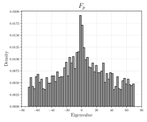
Refer to caption
Refer to caption
Figure 5: Induced subgraph with non-Kesten-McKay e.s.d. We compare the empirical spectral distribution of the induced subgraph Fpsubscript𝐹𝑝F_{p} of Gpsubscript𝐺𝑝G_{p} discussed in Appendix C with that of Gp,{0,g}subscript𝐺𝑝0𝑔G_{p,\{0,g\}} for p=20,021𝑝20021p=$20,021$.
Refer to caption
Figure 6: Minimum eigenvalue of Fpsubscript𝐹𝑝F_{p} subgraph. We plot the minimum eigenvalue of the induced subgraph Fpsubscript𝐹𝑝F_{p} of Gpsubscript𝐺𝑝G_{p} discussed in Appendix C together with the prediction of Conjecture 1.9 (for subgraphs induced by localization, unlike Fpsubscript𝐹𝑝F_{p}) and a conjectural larger scaling of 12p12𝑝-\frac{1}{2}\sqrt{p} that this minimum eigenvalue actually appears to obey closely.