Effect of Coriolis Force on Shear Viscosity : A Non-Relativistic Description

Abstract

We have addressed that during the transition from zero to finite rotation picture, a transition from isotropic to anisotropic nature of shear viscosity coefficients can be found due to Coriolis force as expected due to Lorentz force at a finite magnetic field in earlier studies on the topics of relativistic matter like quark-gluon plasma. We have done it for non-relativistic matters for simplicity, with a future proposal to extend it towards a relativistic description. Introducing the Coriolis force term in relaxation time approximated Boltzmann transport equation, we have found different effective relaxation times along the parallel, perpendicular, and Hall directions in terms of actual relaxation time and rotating time period. Comparing the present formalism with the finite magnetic field picture, we have shown the equivalence of roles between the rotating and cyclotron time periods, which define the rotating time period as the inverse of 2 times angular velocity.

I Introduction

In off-central heavy ion collisions (HIC), a very high orbital angular momentum (OAM) can be deposited. In a typical collision, OAM created from torque at the time of collision could be of the order of $\sim$ ($10^{3}$ - $10^{7}$) $\hbar$, depending on the impact parameter, collision energy, and system size [1, 2, 3]. A fraction of this initial OAM is transferred to the created quark-gluon plasma (QGP) medium in the form of local vorticity. The impact of such a huge initial OAM or later time vorticity on various observables and polarization has been calculated from various theoretical viewpoints. The Refs. [4, 3, 5, 6, 7, 8, 9, 10] have studied the statistical properties with keen interest on the polarization of particles in HIC by demands of angular momentum conservation. Whereas the Refs. [11, 2, 12, 13, 14, 15] have taken the approach of the spin-orbit coupling under strong interactions to explain the polarization observed in HIC. On the other hand, the authors of the Refs. [16, 17, 18, 19, 20, 21, 22, 23, 24, 25, 26, 27, 28, 29, 30, 31, 32] have taken the approach of quantum kinetic theory to obtain chiral anomalies and polarization effects observed in HIC. More recently, a new theoretical framework has been proposed where the complete evolution of spin has been taken care of through explicit incorporation of polarization in a hydrodynamic framework [33, 34, 35, 36, 37, 38, 39, 40, 41, 42, 43]. People have calculated the evolution of vorticity and the polarization of particles with a particular focus on $\Lambda-$hyperon by various transport and hydrodynamical models [44, 45, 46, 47, 48, 49, 50, 51, 52, 53, 54, 55]. See Refs. [56, 36] for recent review papers on the topic related with vorticity of QGP and polarization of hadrons. There is a gross equivalence between the OAM and magnetic field, both of which can be produced in the peripheral collision of heavy ions. Refs. [57, 58] have shown an analogy between the effect of rotation (Coriolis force) and the magnetic field (Lorentz force). Now, the medium constituents (quarks and hadrons) have two basic quantities, momentum, and spin, which will be affected by both OAM and the magnetic field. Former quantity - momentum will get a similar kind of deflection by OAM and magnetic field through Coriolis and Lorentz forces, respectively. On the other hand, the latter quantity - spin will be affected by this OAM (as well as magnetic fields) through a different mechanism, which is basically a matter of focal interest of the spin-hydrodynamics community [56, 36]. This will be ultimately connected with the hot experimental quantity - polarization of hadrons. The present article focuses only on the former quantity - momentum, which will be affected due to the vorticity of the medium via the Coriolis force. Our future aim will be to go for a more realistic picture by considering other ingredients like the effect of other (pseudo) forces due to rotation, the effect of vorticity on the spin, etc. However, the present article is planned to concentrate only on the topic of - the effect of Coriolis force on the shear viscosity of rotating matter. Again for simplicity, we will start with the non-relativistic matter with the future aim to extend it towards a relativistic description.

In recent times, Refs. [59, 60, 61, 62, 63, 64, 65] have gone through a systematic and step by step study on the problem - effect of Lorentz force on shear viscosity of magnetized matter. Connecting the similarity between Lorentz force at a finite magnetic field and Coriolis force at finite vorticity/rotation, the present article is aimed to explore the problem - effect of Coriolis force on shear viscosity of rotating matter. At a finite magnetic field, the (shear) viscous stress tensor breaks into five independent components as one can build five independent velocity gradient tensors in terms of fluid element velocity $u_{i}$ and magnetic field unit vector $b_{i}$. In the absence of magnetic fields, a single velocity gradient component in terms of $u_{i}$ is only possible; hence, one can get an isotropic shear viscosity coefficient of the medium. So, during the transition from zero to finite magnetic field pictures, shear viscosity coefficients transform from isotropic to anisotropic nature. Similarly, viscous stress tensors can have five independent velocity gradient components for a fluid under finite rotation in terms of fluid element velocity $u^{i}$ and angular velocity unit vector $\omega_{i}$. Its detailed formalism part is built in the next section (II), and then in Sec. (III), we have described the numerical outcomes on temperature and angular velocity dependency of shear viscosity with graphical visualization and interpretation. In the end, we have summarized our findings in Sec. (IV).

II Formalism

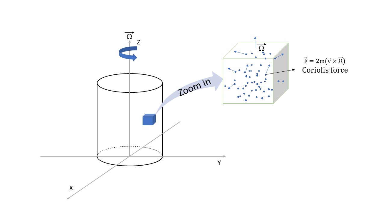
Figure 1: Schematic picture of rotating cylindrical fluid (in the left panel), whose one of the (cubical) fluid elements is zooming in the right panel, where particles inside the fluid element box are randomly moving and facing Coriolis force

In classical mechanics, if we have a system rotating with an angular velocity $\vec{\Omega}$, one can write the following operator equation holding for any arbitrary vector [66],

$$\left(\frac{d}{dt}\right)_{s}\equiv\left(\frac{d}{dt}\right)_{r}+\vec{\Omega}\times~{}~{}~{},$$ (1)

where s and r in the subscripts of the expression mean, the time-derivative of a vector has to be performed with respect to space-fixed and rotating frames, respectively. If one substitutes the position vector $\vec{r}$ in the operator equations one gets the relation,$\vec{v}_{s}=\vec{v}_{r}+\vec{\Omega}\times\vec{r}$, where one identifies $\vec{v}_{s}$ and $\vec{v}_{r}$ with velocity in space-fixed and rotating frame respectively. Again substituting this in general Eq. (1) we have,

$$\vec{a}_{s}=\vec{a}_{r}+2(\vec{\Omega}\times\vec{v}_{r})+\vec{\Omega}\times(\vec{\Omega}\times\vec{r})+\dot{\vec{\Omega}}\times\vec{r}~{}.$$ (2)

We will ignore the subscripts s and r on the vectors for simplicity of notation, so, from now onward, we will call $\vec{v}_{r}$ and its component as $\vec{v}$ and $v_{i}$ respectively. The terms of Eq. (2) can be rearranged to write Newton’s equation in a rotating frame. The second term in Eq. (2) is known as the Coriolis acceleration. In Fig. (1), we have schematically presented a fluid rotating with angular velocity $\vec{\Omega}$. For simple visualization, the geometry of the fluid system has been chosen as cylindrical. If we take any fluid element and look at it closely, the particles inside it have a random part of the velocity $\vec{v}$ on top of the rotational velocity  $\vec{\Omega}\times\vec{r}$. All the particles inside any fluid element feel the Coriolis force $2m(\vec{v}\times\vec{\Omega})$. For the case of constant angular velocity(as is assumed here), the Euler force vanishes, but the other two forces, i.e., Coriolis and Centrifugal, remain non-zero. In the present calculation, we will consider only the effect of Coriolis force on particle motion.
We can find a similarity or equivalence between finite magnetic fields and finite rotation pictures. For example, at finite magnetic field ($B$), a particle with charge $q$ and velocity $v$ will face the Lorentz force $\vec{F}=q\vec{v}\times\vec{B}$, while at angular velocity $\Omega$ of medium, a particle with mass $m$ and velocity $v$ will face the Coriolis force $\vec{F}=2m\vec{v}\times\vec{\Omega}$. The dissipative part of the energy-momentum tensor is modified at the microscopic level through the Lorentz force. A similar kind of modification can be expected for the finite rotation case. The similarity between this finite $B$ and finite $\Omega$ in microscopic descriptions inspire us to build a similar kind of macroscopic description. Refs. [59, 60, 61, 62, 63, 64, 65] have prescribed that macroscopic expressions of dissipative energy-momentum tensor at finite $B$ can be built by the basic tensors - fluid velocity $(u_{i})$, Kronecker delta $(\delta_{ij})$, and the component of magnetic field unit vector, $b_{i}(B_{i}\equiv Bb_{i})$. The same macroscopic structure can be expected in finite rotation by replacing $b_{i}$ by angular velocity unit vector $\omega_{i}(\Omega_{i}\equiv\Omega\omega_{i})$. Following the structure similar to the finite magnetic field case, we can write viscous stress tensor for finite angular velocity as:

$$\tau^{ij}=\eta^{ijkl}U_{kl}~{},$$ (3)

where, $U_{kl}$=$\frac{1}{2}(\frac{\partial u_{k}}{\partial x_{l}}+\frac{\partial u_{l}}{\partial x_{k}})$ is the velocity gradient and $\eta^{ijkl}$ is the viscosity tensor. One can make seven independent tensor components with the properties that they remain symmetric under the exchange of indices $i\leftrightarrow{j}$ and $k\leftrightarrow{l}$ [67]. These tensor components are given below:

$$\delta_{ik}\delta_{jl}+\delta_{jk}\delta_{il},$$

$$\delta_{ij}\delta_{kl},$$

$$\delta_{ik}\omega_{j}\omega_{l}+\delta_{jk}\omega_{i}\omega_{l}+\delta_{il}\omega_{j}\omega_{k}+\delta_{jl}\omega_{i}\omega_{k},$$

$$\delta_{ij}\omega_{k}\omega_{l}+\delta_{kl}\omega_{i}\omega_{j},$$

$$\omega_{i}\omega_{j}\omega_{k}\omega_{l},$$

$$\omega_{ik}\delta_{jl}+\omega_{jk}\delta_{il}+\omega_{il}\delta_{jk}+\omega_{jl}\delta_{ik},$$

$$\omega_{ik}\omega_{j}\omega_{l}+\omega_{jk}\omega_{i}\omega_{l}+\omega_{il}\omega_{j}\omega_{k}+\omega_{jl}\omega_{i}\omega_{k},$$ (4)

where $\omega_{ij}\equiv\epsilon_{ijk}\omega_{k}$. We can make seven independent linear combinations of the above basis to obtain tensors which, when contracted with $U_{kl}$, give five traceless tensors($C^{n}_{ij},n=0\textit{ to }4$) and two non-zero traceless tensors ($C^{n}_{ij},n=5\textit{ to }6$). Similar to the structure of 5 traceless tensors and 2 non-zero traceless tensors for finite magnetic field case [68, 59, 60, 61, 62, 63, 64], they can be expressed as:

$$C_{ijkl}^{0}=(3\omega_{i}\omega_{j}-\delta_{ij})(\omega_{k}\omega_{l}-\frac{1}{3}\delta_{kl})$$

$$C_{ijkl}^{1}=\delta_{il}\delta_{jk}+\delta_{jl}\delta_{ik}-\delta_{ij}\delta_{kl}+\delta_{ij}\omega_{k}\omega_{l}-\delta_{jl}\omega_{i}\omega_{k}$$

$$-\delta_{jk}\omega_{i}\omega_{l}+\delta_{kl}\omega_{i}\omega_{j}-\delta_{ik}\omega_{j}\omega_{l}-\delta_{il}\omega_{j}\omega_{k}+\omega_{i}\omega_{j}\omega_{k}\omega_{l}$$

$$C_{ijkl}^{2}=\delta_{ik}\omega_{j}\omega_{l}+\delta_{il}\omega_{j}\omega_{k}+\delta_{jk}\omega_{i}\omega_{l}+\delta_{jl}\omega_{i}\omega_{k}-4\omega_{i}\omega_{j}\omega_{k}\omega_{l}$$

$$C_{ijkl}^{3}=\delta_{il}\omega_{jk}+\delta_{jl}\omega_{ik}-\omega_{ik}\omega_{j}\omega_{l}-\omega_{jk}\omega_{i}\omega_{l}$$

$$C_{ijkl}^{4}=\omega_{ik}\omega_{j}\omega_{l}+\omega_{il}\omega_{j}\omega_{k}+\omega_{jk}\omega_{i}\omega_{l}+\omega_{jl}\omega_{i}\omega_{k}$$

$$C_{ijkl}^{5}=\delta_{ij}\delta_{kl}$$

$$C_{ijkl}^{6}=\delta_{ij}\omega_{k}\omega_{l}+\delta_{kl}\omega_{i}\omega_{j}~{},$$ (5)

with

$$C_{ij}^{0} = (3\omega_{i}\omega_{j}-\delta_{ij})(\omega_{k}\omega_{l}U_{kl}-\frac{1}{3}\vec{\nabla}\cdot\vec{u})$$

$$C_{ij}^{1} = 2U_{ij}+\delta_{ij}U_{kl}\omega_{k}\omega_{l}-2U_{ik}\omega_{j}\omega_{k}-2U_{jk}\omega_{k}\omega_{i}$$

$$+ (\omega_{i}\omega_{j}-\delta_{ij})\vec{\nabla}\cdot\vec{u}+\omega_{i}\omega_{j}\omega_{k}\omega_{l}U_{kl}$$

$$C_{ij}^{2} = 2(U_{ik}\omega_{j}\omega_{k}+U_{jk}\omega_{i}\omega_{k}-2U_{kl}\omega_{i}\omega_{j}\omega_{k}\omega_{l})$$

$$C_{ij}^{3} = U_{ik}\omega_{jk}+U_{jk}\omega_{ik}-U_{kl}\omega_{ik}\omega_{j}\omega_{l}-U_{kl}\omega_{jk}\omega_{i}\omega_{l}$$

$$C_{ij}^{4} = 2(U_{kl}\omega_{ik}\omega_{j}\omega_{l}+U_{kl}\omega_{jk}\omega_{i}\omega_{l})$$

$$C_{ij}^{5} = \delta_{ij}(\vec{\nabla}\cdot\vec{u})$$

$$C_{ij}^{6} = \delta_{ij}\omega_{k}\omega_{l}U_{kl}+\omega_{i}\omega_{j}(\vec{\nabla}\cdot\vec{u})~{},$$ (6)

where, $C_{ij}^{n}=C^{n}_{ijkl}U_{kl}$. The viscous tensor can be written as a combination of seven basis tensors,

$$\eta_{ijkl}=\eta_{0}{C_{ijkl}}^{0}+\eta_{1}{C_{ijkl}}^{1}+\eta_{2}{C_{ijkl}}^{2}+\eta_{3}{C_{ijkl}}^{3}+\eta_{4}{C_{ijkl}}^{4}+\zeta_{0}{C_{ijkl}}^{5}+\zeta_{1}{C_{ijkl}}^{6}$$ (7)

where, $\eta_{1}\text{ to }\eta_{4}$ are identified as shear viscosities and $\zeta_{0}\text{, and }\zeta_{1}$ are identified with bulk viscosities of the medium. From now onwards, we will concentrate on the shear viscosities of the medium; therefore, we will ignore the bulk part of the viscous stress tensor. So, the viscous stress tensor given in Eq. (3) becomes the shear stress tensor, which can be written as:

$$\pi_{ij} = \eta_{n}C^{n}_{ijkl}U^{kl}$$ (8)

$$= \eta_{n}C^{n}_{ij}~{}.$$

This Eq. (8) is basically the macroscopic expression of shear stress tensor $\pi^{ij}$. For its microscopic expression, we have to use the kinetic theory framework, which can define the dissipative part of the stress tensor as:

$$\pi_{ij}=g\int\frac{d^{3}\vec{p}}{(2\pi)^{3}}mv_{i}v_{j}\delta f~{},$$ (9)

where $g$ is the degeneracy factor of the medium constituent particle with mass $m$ and velocity $v_{i}=p_{i}/m$.

To know the form of $\delta f$, we will use Boltzmann Transport Equation (BTE):

$$\vec{v}\cdot\partialderivative{f}{\vec{r}}+\vec{F}\cdot\frac{\partial f}{\partial\vec{p}}+\frac{\partial f}{\partial t}=\left(\frac{\partial f}{\partial t}\right)_{coll}~{},$$ (10)

where $f$ and $\vec{F}$ are the non-equilibrium distribution function of the particles and the force acting on the particles, respectively. The BTE in relaxation time approximation (RTA) can be written as:

$$\vec{v}\cdot\partialderivative{f}{\vec{r}}+\vec{F}\cdot\frac{\partial f}{\partial\vec{p}}+\frac{\partial f}{\partial t}=-\frac{\delta f}{\tau_{c}}$$ (11)

where the system has been assumed to be slightly out of equilibrium. The total distribution function is composed of two parts- the part corresponding to local equilibrium $f_{0}$ and a perturbed part $\delta f$, i.e., $f=f_{0}+\delta f$. $\tau_{c}$ is the so-called relaxation time for the system. Substituting the expression of Coriolis force in place of $\vec{F}$ and keeping the terms which are 1st order in $\delta f$ in the LHS of Eq. (11) we have,

$$\vec{v}\cdot\partialderivative{f_{0}}{\vec{r}}+2(\vec{v}\times\vec{\Omega})\cdot\frac{\partial\delta f}{\partial\vec{v}}+\frac{\partial f_{0}}{\partial t}=-\frac{\delta f}{\tau_{c}}$$ (12)

where the local equilibrium distribution $f^{0}=1/\exp\Big(\frac{E-\mu(\vec{r},t)-\vec{u}(\vec{r},t)\cdot\vec{p}}{T(\vec{r},t)}\Big{missing})+1$ and $\vec{u}$ is the fluid velocity. By only keeping the terms that correspond to stress in the fluid, the LHS of Eq. (12) can be written as:

$$\frac{mv_{i}v_{j}}{T}\frac{\partial u_{j}}{\partial x_{i}}f_{0}(1-f_{0})+2(\vec{v}\times\vec{\Omega})\cdot\frac{\partial\delta f}{\partial\vec{v}}=-\frac{\delta f}{\tau_{c}}$$ (13)

where we have followed Einstein’s summation convention. Using the identity $U_{ij}\equiv\frac{1}{2}\left(\frac{\partial u_{j}}{\partial x_{i}}+\frac{\partial u_{i}}{\partial x_{j}}\right)$, we can express Eq. (13) as:

$$\frac{m}{T}v_{i}v_{j}U_{ij}f_{0}(1-f_{0})+2(\vec{v}\times\vec{\Omega})\cdot\frac{\partial\delta f}{\partial\vec{v}}=-\frac{\delta f}{\tau_{c}}~{}.$$ (14)

To calculate $\pi_{ij}$, we need $\delta f$, which would be obtained by solving Eq. (14). We will guess the solution of Eq. (14) as:

$$\delta f=\sum_{n=0}^{4}C_{n}C^{n}_{kl}v_{k}v_{l}~{}.$$ (15)

The Eq. (14) can be rewritten as:

$$\frac{m}{T}v_{i}v_{j}U_{ij}f_{0}(1-f_{0})+2\epsilon_{ijk}v_{j}\omega_{k}\Omega\frac{\partial\delta f}{\partial v_{i}} = -\frac{\delta f}{\tau_{c}}$$

$$\implies\frac{m}{T}v_{i}v_{j}U_{ij}f_{0}(1-f_{0})+\frac{1}{\tau_{\Omega}}\omega_{ij}v_{j}\frac{\partial\delta f}{\partial v_{i}} = -\frac{\delta f}{\tau_{c}}~{},$$ (16)

where, $\tau_{\Omega}=\frac{1}{2\Omega}$. We will see later that this $\tau_{\Omega}$ will play same role as the cyclotron time period $\tau_{B}=m/qB$ plays on the transport coefficient expressions at finite magnetic field. Now,

$$\frac{\partial\delta f}{\partial v_{i}}=\frac{\partial}{\partial v_{i}}\sum_{n=o}^{4}C_{n}C^{n}_{kl}v_{k}v_{l}~{}.$$

Using this result of in Eq. (16),

$$\frac{m}{T}v_{i}v_{j}U_{ij}f_{0}(1-f_{0})+\frac{2}{\tau_{\Omega}}\omega_{ij}v_{j}\sum_{n=o}^{4}C_{n}C_{ik}^{n}v_{k}=-\frac{1}{\tau_{c}}\sum_{n=0}^{4}C_{n}C_{kl}^{n}v_{k}v_{l}~{},$$

$$\implies\frac{m}{T}v_{i}v_{j}U_{ij}f_{0}(1-f_{0})=\sum_{n=0}^{4}C_{n}\Big{(}-\frac{2}{\tau_{\Omega}}\omega_{ij}v_{j}v_{k}C_{ik}^{n}-\frac{1}{\tau_{c}}C_{kl}^{n}v_{k}v_{l}\Big{)}~{},$$ (17)

where, $\omega_{ij}v_{i}v_{j}=0$. The Eq. (17) can be further simplified by explicitly expressing $C_{ik}^{n}v_{j}v_{k}$ and $C_{kl}^{n}v_{k}v_{l}$ in terms of elementary tensor structures. All the $C_{n}$’s can be calculated by equating the coefficients of the independent tensor blocks appearing in Eq. (17) to zero. By equating the coefficients $v_{i}v_{j}U_{ij},U_{ij}v_{j}v_{k}\omega_{ik},U_{ij}v_{k}\omega_{j}\omega_{ik}(\vec{v}\cdot\vec{\Omega})$ and $U_{ij}v_{i}\omega_{j}(\vec{v}\cdot\vec{\Omega})$ which occurs in the Eq. (17) to zero, we have respectively,

$$v_{i}v_{j}U_{ij} : -\frac{4C_{3}}{\tau_{\Omega}}-\frac{2C_{1}}{\tau_{c}}=\frac{m}{T}f_{0}(1-f_{0})$$

$$U_{ij}v_{j}v_{k}\omega_{ik} : -\frac{4C_{1}}{\tau_{\Omega}}+\frac{2C_{3}}{\tau_{c}}=0$$

$$U_{ij}v_{k}\omega_{j}\omega_{ik}(\vec{v}\cdot\vec{\Omega}) : \frac{4C_{1}}{\tau_{\Omega}}-\frac{4C_{2}}{\tau_{\Omega}}-\frac{2C_{3}}{\tau_{c}}+\frac{4C_{4}}{\tau_{c}}=0$$

$$U_{ij}v_{i}\omega_{j}(\vec{v}\cdot\vec{\Omega}) : \frac{8C_{3}}{\tau_{\Omega}}-\frac{4C_{4}}{\tau_{\Omega}}+\frac{4C_{1}}{\tau_{c}}-\frac{4C_{2}}{\tau_{c}}=0~{}.$$ (18)

Solving the above set of linear equations we have,

$$C_{1}=-\frac{m}{2T}f_{0}(1-f_{0})\frac{\tau_{c}}{1+4(\tau_{c}/\tau_{\Omega})^{2}}$$

$$C_{2}=-\frac{m}{2T}f_{0}(1-f_{0})\frac{\tau_{c}}{1+(\tau_{c}/\tau_{\Omega})^{2}}$$

$$C_{3}=-\frac{m}{T}f_{0}(1-f_{0})\frac{\tau_{c}(\tau_{c}/\tau_{\Omega})}{1+4(\tau_{c}/\tau_{\Omega})^{2}}$$

$$C_{4}=-\frac{m}{2T}f_{0}(1-f_{0})\frac{\tau_{c}(\tau_{c}/\tau_{\Omega})}{1+4(\tau_{c}/\tau_{\Omega})^{2}}~{}.$$ (19)

Now substituting the value of $\delta f$ in Eq. (9), and using the result $\int v_{i}v_{j}v_{k}v_{l}~{}d^{3}\vec{v}=\frac{v^{4}}{15}(\delta_{ij}\delta_{kl}+\delta_{ik}\delta_{jl}+\delta_{il}\delta_{jk})d^{3}v,(d^{3}v\equiv 4\pi v^{2}dv)$ we have,

$$\pi_{ij}=g\int\frac{d^{3}\vec{p}}{(2\pi)^{3}}m\sum_{n=0}^{4}C_{n}C_{kl}^{n}v_{i}v_{j}v_{k}v_{l}$$

$$\pi_{ij}=g\int{d^{3}v}\frac{m^{4}}{(2\pi)^{3}}\sum_{n=0}^{4}C_{n}C_{kl}^{n}(\delta_{ij}\delta_{kl}+\delta_{ik}\delta_{jl}+\delta_{il}\delta_{jk})\frac{v^{4}}{15}$$

$$\pi_{ij}=\frac{2gm^{4}}{15}\sum_{n=0}^{4}C_{ij}^{n}\int\frac{d^{3}v}{(2\pi)^{3}}v^{4}C_{n}C_{kl}^{n}~{},$$ (20)

where $\delta_{ij}\delta_{kl}+\delta_{ik}\delta_{jl}+\delta_{il}\delta_{jk}=2C_{ij}^{n}$. Substituting the values of $C$’s from Eq. (19) in Eq. (20), we get the corresponding viscosities as,

$$\eta_{n}=-\frac{2gm^{4}}{15}\int\frac{d^{3}v}{(2\pi)^{3}}v^{4}C_{n}~{}.$$ (21)

The $\eta_{0}$ is the viscosity in the absence of rotation, which will be the same to the expression in the absence of magnetic field case; therefore, it is given by [64, 62],

$$\eta_{0}=\frac{g\tau_{c}}{15T}\int\frac{d^{3}p}{(2\pi)^{3}}\frac{p^{4}}{m^{2}}f_{0}(1-f_{0}).$$

And from the Eq. (21) we get,

$$\eta_{1}=\frac{g}{15T}\frac{\tau_{c}}{1+4(\tau_{c}/\tau_{\Omega})^{2}}\int\frac{d^{3}p}{(2\pi)^{3}}\frac{p^{4}}{m^{2}}f_{0}(1-f_{0})$$

$$\eta_{2}=\frac{g}{15T}\frac{\tau_{c}}{1+(\tau_{c}/\tau_{\Omega})^{2}}\int\frac{d^{3}p}{(2\pi)^{3}}\frac{p^{4}}{m^{2}}f_{0}(1-f_{0})$$

$$\eta_{3}=\frac{2g}{15T}\frac{\tau_{c}(\tau_{c}/\tau_{\Omega})}{1+4(\tau_{c}/\tau_{\Omega})^{2}}\int\frac{d^{3}p}{(2\pi)^{3}}\frac{p^{4}}{m^{2}}f_{0}(1-f_{0})$$

$$\eta_{4}=\frac{g}{15T}\frac{\tau_{c}(\tau_{c}/\tau_{\Omega})}{1+(\tau_{c}/\tau_{\Omega})^{2}}\int\frac{d^{3}p}{(2\pi)^{3}}\frac{p^{4}}{m^{2}}f_{0}(1-f_{0})~{}.$$ (22)

Comparing the final expressions of $\eta_{n}$ at finite $\Omega$ with the same for finite $B$, addressed in Refs. [62, 64], the reader can find the similarities in mathematical structure if he equates $\tau_{\Omega}\equiv\tau_{B}$, i.e., $\frac{1}{2\Omega}\equiv\frac{m}{qB}$, which may be understood as an equivalence between Coriolis and Lorentz forces

$${\vec{v}}\times 2m{\vec{\Omega}} \equiv {\vec{v}}\times q{\vec{B}}$$

$$\Rightarrow 2m\Omega \equiv qB~{}.$$ (23)

The above expressions of viscosities can be cast in terms of the Fermi function as follows,

$$\int_{0}^{\infty}dp~{}p^{6}f_{0}(1-f_{0}) = \int_{0}^{\infty}dp~{}p^{6}\left(T\frac{\partial f_{0}}{\partial\mu}\right)$$ (24)

$$= T\frac{\partial}{\partial\mu}\int_{0}^{\infty}dpf_{0}p^{6}$$

$$= 4\sqrt{2}Tm^{7/2}\frac{\partial}{\partial\mu}\int_{0}^{\infty}dEf_{0}E^{5/2}$$

$$= 4\sqrt{2}Tm^{7/2}\frac{\partial}{\partial\mu}\int\frac{E^{(7/2)-1}{dE}}{e^{(E-\mu)/T}+1}$$

$$= 4\sqrt{2}T^{7/2}m^{7/2}\Big{(}T\frac{\partial}{\partial\mu}\int\frac{x^{(7/2)-1}dx}{A^{-1}e^{x}+1}\Big{)},$$

where, $x=E/T$ and $A=e^{\mu/T}.$ The Fermi function is defined as $f_{j}(A)\equiv\frac{1}{\Gamma(j)}\int_{0}^{\infty}\frac{x^{j-1}dx}{A^{-1}e^{x}+1}$, with the property that $\frac{\partial}{\partial(\mu/T)}f_{j}(A)=f_{j-1}(A)$. Using the above definition, we have,

$$\int_{0}^{\infty}dp~{}p^{6}f_{0}(1-f_{0}) =\frac{15}{2}\sqrt{2\pi}m^{7/2}f_{5/2}(A)T^{7/2}.$$ (25)

Using the result of Eq. (25) in Eq. (24) we have,

$$\eta_{1} =g\left(\frac{m}{2\pi}\right)^{3/2}\frac{\tau_{c}}{1+4(\tau_{c}/\tau_{\Omega})^{2}}T^{5/2}f_{5/2}(A)$$

$$\eta_{2} =g\left(\frac{m}{2\pi}\right)^{3/2}\frac{\tau_{c}}{1+(\tau_{c}/\tau_{\Omega})^{2}}T^{5/2}f_{5/2}(A)$$

$$\eta_{3} =g\left(\frac{m}{2\pi}\right)^{3/2}\frac{\tau_{c}(2\tau_{c}/\tau_{\Omega})}{1+4(\tau_{c}/\tau_{\Omega})^{2}}T^{5/2}f_{5/2}(A)$$

$$\eta_{4} =g\left(\frac{m}{2\pi}\right)^{3/2}\frac{\tau_{c}(\tau_{c}/\tau_{\Omega})}{1+(\tau_{c}/\tau_{\Omega})^{2}}T^{5/2}f_{5/2}(A)~{}.$$ (26)

Following the similarity in the definition of parallel, perpendicular, and Hall shear viscosity components $\eta_{\parallel,\perp,\times}$ at finite magnetic field [64, 62], one can define $\eta_{\parallel}=\eta_{1}$, $\eta_{\perp}=\eta_{2}$, $\eta_{\times}=\eta_{4}$.

III Results

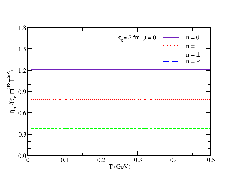
Figure 2: Normalized parallel ($n=\parallel$), perpendicular ($n=\perp$), Hall ($n=\times$) components of shear viscosity as well as shear viscosity without rotation are plotted against temperature axis.

In the previous section (formalism section), we got general expressions of different shear viscosity components for non-relativistic fermionic matter, which can apply to any temperature values $(T)$, chemical potential $(\mu)$ and angular velocity $(\Omega)$. One may readily apply the expression for non-relativistic fluid, belonging to the subject of condensed matter physics and mechanical engineering, where the quantities $T$, $\mu$, and $\Omega$ will be the order of eV in the natural unit. However, our destined system belongs to the subject of high-energy nuclear physics and astrophysics, where MeV will be the order of magnitude for the quantities $T$, $\mu$, and $\Omega$. Imagining the quark-hadron phase transition $T-\mu$ diagram, we can expect two extreme domains - (1) the early universe scenario of net quark/baryon-free domain (i.e., at $\mu=0$), which can be produced in LHC and RHIC experiments, and (2) the compact star scenario of degenerate electron or neutron or quark matter (i.e., at $T=0$), expected in white dwarfs and neutron stars. Our microscopic expressions of shear viscosity components at finite rotation can be easily applicable to RHIC/LHC matter by putting $\mu=0$ and to compact star by putting $T=0$ in the general forms of Eq. (26). Although, we have limitations for using non-relativistic matter, which can provide some overestimation with respect to the actual relativistic matter expected in RHIC/LHC experiments and compact stars. Our future goal is to reach that actual scenario by developing the framework in step by step. By putting $\mu=0$ and $A=e^{\mu/T}=1$ in Eq. (26), we get

$$\eta_{\parallel}=\eta_{1} =0.64g\left(\frac{m}{2\pi}\right)^{3/2}\frac{\tau_{c}}{1+4(\tau_{c}/\tau_{\Omega})^{2}}T^{5/2}\zeta(5/2)$$

$$\eta_{\perp}=\eta_{2} =0.64g\left(\frac{m}{2\pi}\right)^{3/2}\frac{\tau_{c}}{1+(\tau_{c}/\tau_{\Omega})^{2}}T^{5/2}\zeta(5/2)$$

$$\eta_{\times}=\eta_{4} =0.64g\left(\frac{m}{2\pi}\right)^{3/2}\frac{\tau_{c}(\tau_{c}/\tau_{\Omega})}{1+(\tau_{c}/\tau_{\Omega})^{2}}T^{5/2}\zeta(5/2)$$ (27)

as Fermi function become $f_{5/2}(A=1)=(1-\frac{1}{2^{3/2}})\zeta(5/2)$. Using Eq. (27), we have plotted $\eta_{||,\perp,\times}/\tau_{c}m^{3/2}T^{5/2}$ against $T$-axis in Fig. (2) and we get horizontal lines as all components are proportional to $T^{5/2}$. We consider quark matter with mass, $m=0.005GeV$ and relaxation time $\tau_{c}=5fm$ and angular time period $\tau_{\Omega}=35~{}GeV^{-1}=6.8fm$ for angular velocity $\Omega=\frac{1}{2\tau_{\Omega}}=0.014GeV$. We keep comparable values of two-time scales, for which we can get a noticeable difference between parallel and perpendicular components of shear viscosity.

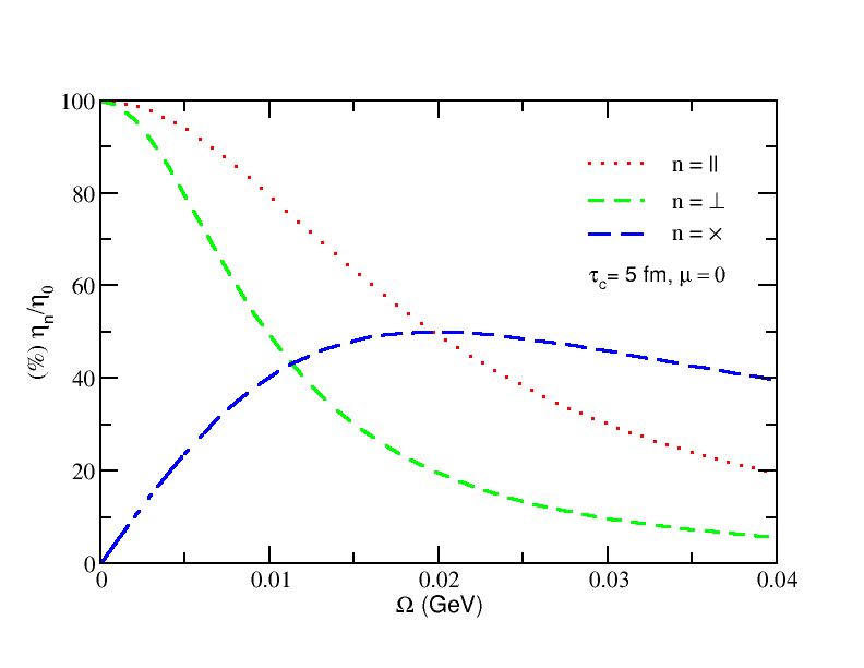
Figure 3: Relative percentage of parallel ($n=\parallel$), perpendicular ($n=\perp$), Hall ($n=\times$) components of shear viscosity vs angular velocity.

We can understand the $\eta_{\parallel,\perp,\times}$ in terms of effective relaxation time

$$\tau_{\parallel} =\frac{\tau_{c}}{1+4(\tau_{c}/\tau_{\Omega})^{2}}$$

$$\tau_{\perp} =\frac{\tau_{c}}{1+(\tau_{c}/\tau_{\Omega})^{2}}$$

$$\tau_{\times} =\frac{\tau_{c}(\tau_{c}/\tau_{\Omega})}{1+(\tau_{c}/\tau_{\Omega})^{2}}$$ (28)

as $\eta_{\parallel,\perp,\times}\propto\tau_{\parallel,\perp,\times}$, while $\eta_{0}\propto\tau_{c}$ only. So we can easily understand that the non-zero ratio $\tau_{c}/\tau_{\Omega}$ for finite rotation will create the inequality $\tau_{\parallel,\perp,\times}<\tau_{c}$ and the ratio is also the deciding factor for the ranking among $\eta_{\parallel}$, $\eta_{\perp}$, $\eta_{\times}$. In Fig. (2), for present set of parameters $\tau_{c}=5fm$, $\tau_{\Omega}=6.8fm$ and ratio $\tau_{c}/\tau_{\Omega}=0.73$, we get the ranking $\eta_{\parallel}>\eta_{\times}>\eta_{\perp}$ but it can be changed for different values of the ratio $\tau_{c}/\tau_{\Omega}$. This fact will be more clear in the next plot.

In Fig. (3), we have plotted the percentage of normalized viscosities ($\eta_{n}/\eta_{0}$) with respect to $\Omega$ at $\tau_{c}=5fm$. It is clearly seen in the plot that the relative magnitude of $\eta_{\perp,||}$ decreases with $\Omega$ in the whole range, whereas $\eta_{\times}$ initially increases and then decreases with $\Omega$. In the lower range of $\Omega$, $\eta_{\perp,||}$ are more dominant than $\eta_{\times}$, on contrary in higher range of $\Omega$, $\eta_{\times}$ is more dominant than $\eta_{\perp,||}$. One can identify both $\eta_{\perp,||}$ will merge to $\eta_{0}$ in the absence of vorticity, i.e, $\eta_{\perp,||}(\Omega\xrightarrow{}0)=\eta_{0}$. From this fact, we can conclude that the finite (global) vorticity can create anisotropy in shear viscosity components, as we have noticed in the finite magnetic field picture.

Let us try to visualize the different shear viscosity components via a schematic diagram - Fig. (4). The picture is precisely similar to the finite magnetic field picture described in Refs. [69]. Only the direction of the magnetic field along the z-direction will be replaced by the direction of orbital angular momentum or angular velocity, or global vorticity. In Fig. (4), the arrows represent the velocity direction, and their lengths represent their magnitudes, so changing the arrow lengths map the velocity gradient picture. Right, and left panels of Fig. (4) represent the gradient of velocity in the planes, which are parallel (ZX and ZY plane) and perpendicular (XY plane) to the vorticity/angular velocity, respectively.

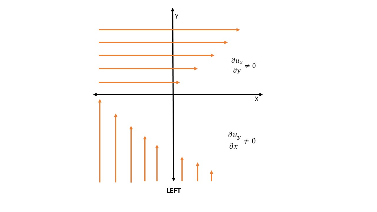
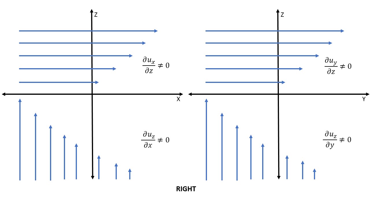
Figure 4: Velocity gradients along the axis of XY, ZX and ZY plane

Apart from the rotating quark matter system at $\mu=0$, we can apply the microscopic expressions in Eq. (27) for rotating hadronic matter at $\mu=0$, although the magnitude of angular momentum will be reduced to a smaller value in hadronic phase expansion. Considering the $T\rightarrow 0$ limit of Eq. (26), we can get

$$\eta_{\parallel}=\eta_{1} =\frac{8g}{15\sqrt{\pi}}\left(\frac{m}{2\pi}\right)^{3/2}\frac{\tau_{c}}{1+4(\tau_{c}/\tau_{\Omega})^{2}}\mu^{5/2}$$

$$\eta_{\perp}=\eta_{2} =\frac{8g}{15\sqrt{\pi}}\left(\frac{m}{2\pi}\right)^{3/2}\frac{\tau_{c}}{1+(\tau_{c}/\tau_{\Omega})^{2}}\mu^{5/2}$$

$$\eta_{\times}=\eta_{4} =\frac{8g}{15\sqrt{\pi}}\left(\frac{m}{2\pi}\right)^{3/2}\frac{\tau_{c}(\tau_{c}/\tau_{\Omega})}{1+(\tau_{c}/\tau_{\Omega})^{2}}\mu^{5/2}~{},$$ (29)

which may be applicable for rotating compact star systems like white dwarfs, neutron stars, and quark matter (expected in the core of a neutron star). However, an over-estimation of shear viscosity components of those rotating media can be expected due to considering the non-relativistic description of relativistic matter. This fact can be understood from the Fig. (5), where the relativistic and non-relativistic velocity $(v)$ of u quark, pion, and nucleon are plotted against momentum $(p)$. From this simple picture, one can see the noticeable difference between relativistic (R) and non-relativistic (NR) curves are coming beyond the threshold momenta $1MeV$, $30MeV$ and $300MeV$ for u quark, $\pi$ meson and nucleon respectively. Overestimation in NR description with respect to R description will come for integration of momentum beyond those threshold values. Our future aim is to go for that relativistic description with an appropriate relativistic extension of the present framework.

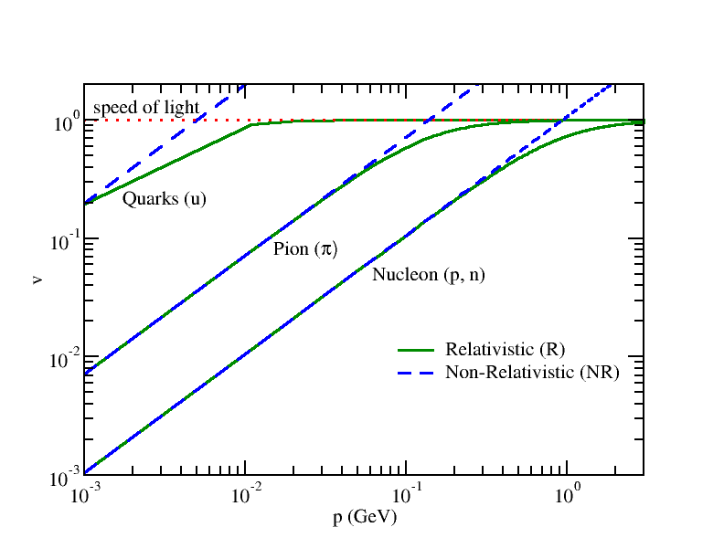
Figure 5: Velocity ($v$) vs momentum ($p$) relation for u quark, $\pi$ meson and nucleons.

Regarding the fluidity of the medium, quantified by shear viscosity to entropy density ratio, we can find a possibility of violation of KSS bound [70] due to rotation of medium via Coriolis force just like finite magnetic field picture via Lorentz force. The entropy density of non-relativistic matter in two extreme limits follow the relations - $s\propto T^{3/2}$ at $\mu\rightarrow 0$and $s\propto\mu^{3/2}$ at $T\rightarrow 0$. The ratio between shear viscosity to entropy density will be $\eta/s=\frac{\tau_{c}T}{5}$ at $\mu\rightarrow 0$ and $\eta/s=\frac{\tau_{c}\mu}{5}$ at $T\rightarrow 0$, which can reach to the KSS bound $\frac{1}{4\pi}$ [70] for relaxation time $\tau_{c}(T)=\frac{5}{4\pi T}$ and $\tau_{c}(\mu)=\frac{5}{4\pi\mu}$ respectively. At finite rotation, we can expect lower limit expressions for parallel, perpendicular, and Hall components of shear viscosity to entropy density ratio as,

$$\frac{\eta_{\parallel}}{s} = \frac{1}{4\pi}\frac{1}{1+4\Big{(}\frac{5}{4\pi T\tau_{\Omega}}\Big{)}^{2}}$$

$$\frac{\eta_{\perp}}{s} = \frac{1}{4\pi}\frac{1}{1+\Big{(}\frac{5}{4\pi T\tau_{\Omega}}\Big{)}^{2}}$$

$$\frac{\eta_{\times}}{s} = \frac{1}{4\pi}\frac{\Big{(}\frac{5}{4\pi T\tau_{\Omega}}\Big{)}}{1+\Big{(}\frac{5}{4\pi T\tau_{\Omega}}\Big{)}^{2}}~{}.$$ (30)

The above expressions are for $\mu=0$. By replacing $T$ by $\mu$ in Eq. (30), one can get their corresponding expression for $T=0$. So, one can notice that by increasing angular velocity or decreasing $\tau_{\Omega}$ of the medium, $\eta_{\parallel,\perp}/s$ can go below $\frac{1}{4\pi}$. The $\eta_{\parallel}/s<1/(4\pi)$ is also expected and pointed out by Ref. [71] for finite magnetic field. As a matter of fact, a quantum version extension of the present formalism may be required to comment something on the lower bounds of $\eta_{\parallel,\perp}/s$.

IV Summary

In summary, we have explored the equivalence role of magnetic field and rotation or vorticity on shear viscosity via Lorentz force and Coriolis force, respectively. In the absence of magnetic fields or rotation, we get an isotropic shear viscosity coefficient, which is proportional to relaxation time only. Whereas at finite magnetic field or rotation, we get anisotropic shear viscosity coefficients, which are proportional to effective relaxation time along the parallel, perpendicular, and Hall directions. This effective relaxation time can be expressed in terms of actual relaxation time and cyclotron-type time period due to magnetic field or rotation. The physics and mathematical steps of the microscopic calculation of shear viscosity at a finite magnetic field or rotation are pretty similar. The microscopic quantity - the deviation from equilibrium distribution, is due to the macroscopic velocity gradient, so a proportional relation between them is considered with unknown proportionality constants, which have been calculated with the help of the relaxation time approximation of the Boltzmann transport equation. Then, the macroscopic relation between the shear stress tensor and velocity gradient with shear viscosity proportional constants is compared with the microscopic expression of the shear stress tensor in terms of deviation obtained from the Boltzmann transport equation. By this comparison, we get isotropic and anisotropic shear viscosities in terms of relaxation time and effective relaxation time in the absence and presence of magnetic fields or rotation. We generally obtain the deviation from the Boltzmann transport equation using Lorentz force for finite magnetic field case. The same is done here by including the Coriolis force for the finite rotation case. The present article has explored the detailed calculation of the finite rotation case only. During the description, we have also mentioned the equivalence with the finite magnetic field case. For simplicity, we have attempted it for non-relativistic matter but our immediate future plan is to extend it towards relativistic description. So far, to the best of our knowledge, it is the first time that we have addressed this anisotropic structure of shear viscosity of rotating matter due to the Coriolis force. We have noticed an equivalence role between the rotating time period for finite rotation case and cyclotron time period for finite magnetic field case, where the rotating time period is defined as the inverse of 2 times angular velocity. The factor 2 propagates from the basic definition of the Coriolis force.

References

- Adamczyk et al. [2017] L. Adamczyk et al. (STAR), Nature 548, 62 (2017), arXiv:1701.06657 [nucl-ex] .
- Liang and Wang [2005a] Z.-T. Liang and X.-N. Wang, Phys. Rev. Lett. 94, 102301 (2005a), [Erratum: Phys.Rev.Lett. 96, 039901 (2006)], arXiv:nucl-th/0410079 .
- Becattini et al. [2008] F. Becattini, F. Piccinini, and J. Rizzo, Phys. Rev. C 77, 024906 (2008), arXiv:0711.1253 [nucl-th] .
- Becattini and Ferroni [2007] F. Becattini and L. Ferroni, The European Physical Journal C 52, 597 (2007).
- Becattini and Piccinini [2008] F. Becattini and F. Piccinini, Annals of Physics 323, 2452 (2008).
- Becattini and Tinti [2010] F. Becattini and L. Tinti, Annals of Physics 325, 1566 (2010).
- Becattini et al. [2013a] F. Becattini, V. Chandra, L. Del Zanna, and E. Grossi, Annals Phys. 338, 32 (2013a), arXiv:1303.3431 [nucl-th] .
- Becattini et al. [2013b] F. Becattini, L. Csernai, and D. J. Wang, Phys. Rev. C 88, 034905 (2013b), [Erratum: Phys.Rev.C 93, 069901 (2016)], arXiv:1304.4427 [nucl-th] .
- Becattini et al. [2015] F. Becattini, G. Inghirami, V. Rolando, A. Beraudo, L. Del Zanna, A. De Pace, M. Nardi, G. Pagliara, and V. Chandra, Eur. Phys. J. C 75, 406 (2015), [Erratum: Eur.Phys.J.C 78, 354 (2018)], arXiv:1501.04468 [nucl-th] .
- Becattini et al. [2021] F. Becattini, M. Buzzegoli, and A. Palermo, Phys. Lett. B 820, 136519 (2021), arXiv:2103.10917 [nucl-th] .
- Betz et al. [2007] B. Betz, M. Gyulassy, and G. Torrieri, Phys. Rev. C 76, 044901 (2007), arXiv:0708.0035 [nucl-th] .
- Liang and Wang [2005b] Z.-T. Liang and X.-N. Wang, Physics Letters B 629, 20 (2005b).
- Gao et al. [2008] J.-H. Gao, S.-W. Chen, W.-t. Deng, Z.-T. Liang, Q. Wang, and X.-N. Wang, Phys. Rev. C 77, 044902 (2008).
- Chen et al. [2009] S.-w. Chen, J. Deng, J.-h. Gao, and Q. Wang, Frontiers of Physics in China 4, 509 (2009).
- Huang et al. [2011a] X.-G. Huang, P. Huovinen, and X.-N. Wang, Phys. Rev. C 84, 054910 (2011a).
- Gao et al. [2012] J.-H. Gao, Z.-T. Liang, S. Pu, Q. Wang, and X.-N. Wang, Phys. Rev. Lett. 109, 232301 (2012).
- Chen et al. [2013] J.-W. Chen, S. Pu, Q. Wang, and X.-N. Wang, Phys. Rev. Lett. 110, 262301 (2013).
- Fang et al. [2016] R.-h. Fang, L.-g. Pang, Q. Wang, and X.-n. Wang, Phys. Rev. C 94, 024904 (2016).
- Fang et al. [2017] R.-h. Fang, J.-y. Pang, Q. Wang, and X.-n. Wang, Phys. Rev. D 95, 014032 (2017).
- hua Gao and Wang [2015] J. hua Gao and Q. Wang, Physics Letters B 749, 542 (2015).
- Hidaka et al. [2017] Y. Hidaka, S. Pu, and D.-L. Yang, Phys. Rev. D 95, 091901 (2017).
- Gao et al. [2017] J.-h. Gao, S. Pu, and Q. Wang, Phys. Rev. D 96, 016002 (2017).
- Gao et al. [2018] J.-H. Gao, Z.-T. Liang, Q. Wang, and X.-N. Wang, Phys. Rev. D 98, 036019 (2018).
- Huang et al. [2018] A. Huang, S. Shi, Y. Jiang, J. Liao, and P. Zhuang, Phys. Rev. D 98, 036010 (2018).
- Gao et al. [2019] J.-H. Gao, J.-Y. Pang, and Q. Wang, Phys. Rev. D 100, 016008 (2019).
- Gao and Liang [2019] J.-H. Gao and Z.-T. Liang, Phys. Rev. D 100, 056021 (2019).
- Hattori et al. [2019] K. Hattori, Y. Hidaka, and D.-L. Yang, Phys. Rev. D 100, 096011 (2019).
- Wang et al. [2019] Z. Wang, X. Guo, S. Shi, and P. Zhuang, Phys. Rev. D 100, 014015 (2019).
- Weickgenannt et al. [2019] N. Weickgenannt, X.-l. Sheng, E. Speranza, Q. Wang, and D. H. Rischke, Phys. Rev. D 100, 056018 (2019).
- Yang et al. [2020] D.-L. Yang, K. Hattori, and Y. Hidaka, Journal of High Energy Physics 2020, 1 (2020).
- Weickgenannt et al. [2021a] N. Weickgenannt, E. Speranza, X.-l. Sheng, Q. Wang, and D. H. Rischke, Phys. Rev. Lett. 127, 052301 (2021a).
- Weickgenannt et al. [2021b] N. Weickgenannt, E. Speranza, X.-l. Sheng, Q. Wang, and D. H. Rischke, Phys. Rev. D 104, 016022 (2021b).
- Becattini [2011] F. Becattini, Physics of Particles and Nuclei Letters 8, 801 (2011).
- Florkowski et al. [2018a] W. Florkowski, B. Friman, A. Jaiswal, and E. Speranza, Phys. Rev. C 97, 041901 (2018a).
- Florkowski et al. [2018b] W. Florkowski, B. Friman, A. Jaiswal, R. Ryblewski, and E. Speranza, Phys. Rev. D 97, 116017 (2018b).
- Florkowski et al. [2019a] W. Florkowski, A. Kumar, and R. Ryblewski, Prog. Part. Nucl. Phys. 108, 103709 (2019a), arXiv:1811.04409 [nucl-th] .
- Florkowski et al. [2018c] W. Florkowski, A. Kumar, and R. Ryblewski, Phys. Rev. C 98, 044906 (2018c), arXiv:1806.02616 [hep-ph] .
- Becattini et al. [2019] F. Becattini, W. Florkowski, and E. Speranza, Physics Letters B 789, 419 (2019).
- Florkowski et al. [2019b] W. Florkowski, A. Kumar, R. Ryblewski, and R. Singh, Phys. Rev. C 99, 044910 (2019b), arXiv:1901.09655 [hep-ph] .
- Bhadury et al. [2021a] S. Bhadury, W. Florkowski, A. Jaiswal, A. Kumar, and R. Ryblewski, Physics Letters B 814, 136096 (2021a).
- Bhadury et al. [2021b] S. Bhadury, W. Florkowski, A. Jaiswal, A. Kumar, and R. Ryblewski, Phys. Rev. D 103, 014030 (2021b).
- Daher et al. [2022] A. Daher, A. Das, W. Florkowski, and R. Ryblewski, arXiv preprint arXiv:2202.12609 (2022).
- Bhadury et al. [2022] S. Bhadury, W. Florkowski, A. Jaiswal, A. Kumar, and R. Ryblewski, Phys. Rev. Lett. 129, 192301 (2022).
- Deng and Huang [2016] W.-T. Deng and X.-G. Huang, Phys. Rev. C 93, 064907 (2016), arXiv:1603.06117 [nucl-th] .
- Jiang et al. [2016] Y. Jiang, Z.-W. Lin, and J. Liao, Phys. Rev. C 94, 044910 (2016).
- Pang et al. [2016] L.-G. Pang, H. Petersen, Q. Wang, and X.-N. Wang, Phys. Rev. Lett. 117, 192301 (2016), arXiv:1605.04024 [hep-ph] .
- Li et al. [2017] H. Li, L.-G. Pang, Q. Wang, and X.-L. Xia, Phys. Rev. C 96, 054908 (2017), arXiv:1704.01507 [nucl-th] .
- Xia et al. [2018] X.-L. Xia, H. Li, Z.-B. Tang, and Q. Wang, Phys. Rev. C 98, 024905 (2018), arXiv:1803.00867 [nucl-th] .
- Wei et al. [2019] D.-X. Wei, W.-T. Deng, and X.-G. Huang, Phys. Rev. C 99, 014905 (2019), arXiv:1810.00151 [nucl-th] .
- Huang [2021] X.-G. Huang, Nucl. Phys. A 1005, 121752 (2021), arXiv:2002.07549 [nucl-th] .
- Wu et al. [2021] H.-Z. Wu, L.-G. Pang, X.-G. Huang, and Q. Wang, Nucl. Phys. A 1005, 121831 (2021), arXiv:2002.03360 [nucl-th] .
- Huang et al. [2021] X.-G. Huang, J. Liao, Q. Wang, and X.-L. Xia, Lect. Notes Phys. 987, 281 (2021), arXiv:2010.08937 [nucl-th] .
- Fu et al. [2021] B. Fu, S. Y. F. Liu, L. Pang, H. Song, and Y. Yin, Phys. Rev. Lett. 127, 142301 (2021), arXiv:2103.10403 [hep-ph] .
- Deng et al. [2022] X.-G. Deng, X.-G. Huang, and Y.-G. Ma, Physics Letters B 835, 137560 (2022).
- Li et al. [2022] H. Li, X.-L. Xia, X.-G. Huang, and H. Z. Huang, Physics Letters B 827, 136971 (2022).
- Becattini and Lisa [2020] F. Becattini and M. A. Lisa, Ann. Rev. Nucl. Part. Sci. 70, 395 (2020), arXiv:2003.03640 [nucl-ex] .
- Sivardiere [1983] J. Sivardiere, European Journal of Physics 4, 162 (1983).
- Johnson [2000] B. L. Johnson, Am. J. Phys. 68, 649 (2000).
- Tuchin [2012] K. Tuchin, J. Phys. G 39, 025010 (2012), arXiv:1108.4394 [nucl-th] .
- Ghosh et al. [2019] S. Ghosh, B. Chatterjee, P. Mohanty, A. Mukharjee, and H. Mishra, Phys. Rev. D 100, 034024 (2019), arXiv:1804.00812 [hep-ph] .
- Mohanty et al. [2019] P. Mohanty, A. Dash, and V. Roy, Eur. Phys. J. A 55, 35 (2019), arXiv:1804.01788 [nucl-th] .
- Dey et al. [2021a] J. Dey, S. Satapathy, A. Mishra, S. Paul, and S. Ghosh, Int. J. Mod. Phys. E 30, 2150044 (2021a), arXiv:1908.04335 [hep-ph] .
- Dash et al. [2020] A. Dash, S. Samanta, J. Dey, U. Gangopadhyaya, S. Ghosh, and V. Roy, Phys. Rev. D 102, 016016 (2020), arXiv:2002.08781 [nucl-th] .
- Dey et al. [2021b] J. Dey, S. Satapathy, P. Murmu, and S. Ghosh, Pramana 95, 125 (2021b), arXiv:1907.11164 [hep-ph] .
- Ghosh and Ghosh [2021] S. Ghosh and S. Ghosh, Phys. Rev. D 103, 096015 (2021), arXiv:2011.04261 [hep-ph] .
- Goldstein [2011] H. Goldstein, Classical mechanics (Pearson Education India, 2011).
- Huang et al. [2011b] X.-G. Huang, A. Sedrakian, and D. H. Rischke, Annals of Physics 326, 3075 (2011b).
- Pitaevskii et al. [2017] L. Pitaevskii, E. Lifshitz, and J. B. Sykes, Course of theoretical physics: physical kinetics, Vol. 10 (Elsevier, 2017).
- Hattori et al. [2022] K. Hattori, M. Hongo, and X.-G. Huang, Symmetry 14, 1851 (2022), arXiv:2207.12794 [hep-th] .
- Kovtun et al. [2005] P. Kovtun, D. T. Son, and A. O. Starinets, Phys. Rev. Lett. 94, 111601 (2005), arXiv:hep-th/0405231 .
- Critelli et al. [2014] R. Critelli, S. I. Finazzo, M. Zaniboni, and J. Noronha, Phys. Rev. D 90, 066006 (2014), arXiv:1406.6019 [hep-th] .