Wide binary stars formed in the turbulent interstellar medium

Abstract

The ubiquitous interstellar turbulence regulates star formation and the scaling relations between the initial velocity differences and the initial separations of stars. We propose that the formation of wide binaries with initial separations $r$ in the range $\sim 10^{3}~{}\text{AU}\lesssim r\lesssim 10^{5}$ AU is a natural consequence of star formation in the turbulent interstellar medium. With the decrease of $r$, the mean turbulent relative velocity $v_{\text{tur}}$ between a pair of stars decreases, while the largest velocity $v_{\text{bon}}$ at which they still may be gravitationally bound increases. When $v_{\text{tur}}<v_{\text{bon}}$, a wide binary can form. In this formation scenario, we derive the eccentricity distribution $p(e)$ of wide binaries for an arbitrary relative velocity distribution. By adopting a turbulent velocity distribution, we find that wide binaries at a given initial separation generally exhibit a superthermal $p(e)$. This provides a natural explanation for the observed superthermal $p(e)$ of the wide binaries in the Solar neighbourhood.

1 Introduction

Gaia (Gaia Collaboration et al., 2016, 2019) has revealed a large number of wide binaries with semimajor axes $a\gtrsim 10^{3}~{}$AU (e.g., El-Badry & Rix 2018; Igoshev & Perets 2019; Hwang et al. 2020; Tian et al. 2020; Hartman & Lépine 2020; El-Badry et al. 2021). Due to their sensitivity to gravitational perturbations, wide binaries have been used to probe unseen Galactic disk material (Bahcall et al., 1985), dark matter substructure (Peñarrubia et al., 2016), MAssive Compact Halo Objects (MACHOs, Chanamé & Gould 2004; Quinn et al. 2009; Monroy-Rodríguez & Allen 2014), and constrain the dynamical history of the Galaxy (Allen et al., 2007; Hwang et al., 2022b).

Despite their important astrophysical implications, the origin of wide binaries remains a mystery. Due to their large $a$’s (comparable to the typical size $\sim 0.1~{}$ pc $\approx 2\times 10^{4}$ AU of molecular cores, Ward-Thompson et al. 2007) and the dynamical disruption in star clusters, it is believed that very wide binaries with $a\gtrsim 0.1~{}$pc can hardly form and survive in dense star-forming regions (Deacon & Kraus, 2020). Various wide-binary formation mechanisms have been proposed, including cluster dissolution (Kouwenhoven et al., 2010; Moeckel & Clarke, 2011), dynamical unfolding of compact triple systems (Reipurth & Mikkola, 2012), formation in adjacent cores with a small relative velocity (Tokovinin, 2017), and in the tidal tails of stellar clusters (Peñarrubia, 2021; Livernois et al., 2023). Observations of the large fraction of wide pairs of young stars in low-density star-forming regions (Tokovinin, 2017), the chemical homogeneity between the components of wide binaries (Hawkins et al., 2020), the metallicity dependence of the wide-binary fraction (Hwang et al., 2021), and N-body simulations (e.g., Kroupa & Burkert 2001) suggest that wide binary-components are likely to form in the same star-forming region (Andrews et al., 2019).

In addition, Gaia’s high-precision astrometric measurements reveal superthermal eccentricity distribution for wide binaries with separations $\gtrsim 10^{3}$ AU (Tokovinin, 2020; Hwang et al., 2022a). Hamilton (2022) suggests that a superthermal eccentricity distribution cannot be produced dynamically, implying that the initial distribution must itself be superthermal.

The interstellar medium (ISM) and star-forming regions are turbulent, with the turbulent energy mainly coming from supernova explosions (Padoan et al., 2016). The observationally measured power-law spectrum of turbulence spans many orders of magnitude in length scales, from $\sim 100$ pc down to $\sim 10^{-11}$ pc in the warm ionized medium (e.g., Armstrong et al. 1995; Chepurnov & Lazarian 2010; Xu & Zhang 2017, 2020) and down to $\sim 0.01$ pc in molecular clouds (MCs) (Lazarian, 2009; Hennebelle & Falgarone, 2012; Yuen et al., 2022). The ubiquitous turbulence plays a fundamental role in the modern star formation paradigm (Mac Low & Klessen, 2004; Elmegreen & Scalo, 2004; McKee & Ostriker, 2007). Our understanding of star formation has significantly improved thanks to the recent development in theories of magnetohydrodynamic (MHD) turbulence (Goldreich & Sridhar, 1995; Lazarian & Vishniac, 1999; Cho & Lazarian, 2002), MHD simulations (e.g., Stone et al. 1998; Federrath et al. 2011; Padoan et al. 2016; Kritsuk et al. 2017), and techniques for measuring interstellar turbulence (e.g., Lazarian & Pogosyan 2000; Heyer & Brunt 2004; Lazarian & Pogosyan 2006; Lazarian et al. 2018; Xu & Hu 2021; Burkhart 2021).

Turbulence not only regulates the dynamics of MCs and the formation of density structures, e.g., filaments, clumps, and cores, where star formation takes place, but also affects the kinematics of molecular gas and dust (Hennebelle & Falgarone, 2012), density structures, and young stars over a broad range of length scales. Dense cores in MCs (Qian et al., 2018; Xu, 2020) and young stars (Ha et al., 2021; Krolikowski et al., 2021; Zhou et al., 2021; Ha et al., 2022) inherit their velocities from the surrounding turbulent gas, and thus the statistical properties of their velocities are similar to that of the turbulent gas.

In this letter, we will investigate how the initial turbulent velocities between pairs of stars affect the formation of wide binaries and their eccentricities. We first describe the initial turbulent velocities of pairs of stars in Section 2. In Section 3, we focus on the formation of wide binaries and their eccentricity distribution. More discussion is provided in Section 4. Our conclusions follow in Section 5.

2 Initial turbulent velocities of stars

Stars form in high-density structures, i.e., filaments, cores, in turbulent MCs, which are generated by the compressions and shocks in highly supersonic turbulence (Federrath et al., 2009; Mocz & Burkhart, 2018; Inoue et al., 2018; Xu et al., 2019). Dense cores arise at the collision interfaces of converging turbulent flows, with turbulent motions existing on sub-core scales (Volgenau, 2004). Naturally, the turbulent velocities of gas are imprinted in those of newly formed stars. As confirmed by recent Gaia observations (e.g., Ha et al. 2021; Zhou et al. 2021; Ha et al. 2022), the velocity differences and spatial separations of young stars statistically follow the power-law velocity scaling of interstellar turbulence.

We consider that in a star-forming region, the initial velocity differences and spatial separations of stars at birth statistically satisfy the averaged turbulent velocity scaling,

$$v_{\text{tur}}=\langle v\rangle=V_{L}\Big{(}\frac{r}{L}\Big{)}^{\alpha},$$ (1)

where $r$ is the initial separation between a pair of stars, and $v$ is the absolute value of their initial velocity difference. The injected turbulent speed $V_{L}$ and the injection scale $L$ have typical values as $\sim 10~{}\text{km}~{}\text{s}^{-1}$ and $\sim 100~{}\text{pc}$ for interstellar turbulence (Chamandy & Shukurov, 2020). The power-law index $\alpha$ reflects the properties of turbulence, which is typically $1/3$ for solenoidal turbulent motions with the Kolmogorov scaling, and close to $1/2$ for highly compressive turbulent motions dominated by shocks (Federrath et al., 2009; Kowal & Lazarian, 2010). A steeper turbulent velocity scaling (i.e., a larger $\alpha$) corresponds to a more efficient energy dissipation in shock-dominated turbulence. The Kolmogorov scaling applies to most of the volume of an MC, while the steeper scaling is preferentially seen in small-scale high-density regions that result from shock compressions (Lazarian, 2009; Xu, 2020; Xu & Hu, 2021; Rani et al., 2022; Yuen et al., 2022).

In Fig. 1, we illustrate the 3D distribution of gas velocities $v_{t}$ taken from MHD turbulence simulations in physical conditions similar to those of a star-forming region (Hu et al., 2021), with the sonic Mach number $M_{s}=V_{L}/c_{s}\approx 10$ and Alfvén Mach number $M_{A}=V_{L}/V_{A}\approx 0.5$, where $c_{s}$ is the sound speed, and $V_{A}$ is the Alfvén speed. The grid resolution is $792^{3}$, $L$ is about half of the box size, and $V_{L}\approx 3$ (numerical unit). By using the turbulent velocities from the simulation, we measure the speed distribution $f(v)$ (such that $\int f(v)dv=1$) corresponding to different $r$’s and present it in Fig. 1. It approximately follows

$$f(v)\approx\sqrt{\frac{2}{\pi}}\frac{1}{\sigma_{v}^{3}}\exp{\Big{(}-\frac{v^{2}}{2\sigma_{v}^{2}}\Big{)}}v^{2}.$$ (2)

We find that the parameter $\sigma_{v}$ is comparable to $v_{\text{tur}}$ (Eq. (1)). The dashed lines in Fig. 1 represent $f(v)$ given by Eq. (2) with $\sigma_{v}\approx 0.7v_{\text{tur}}$ and $\alpha=1/3$, which approximately agree with the numerical results.

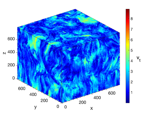
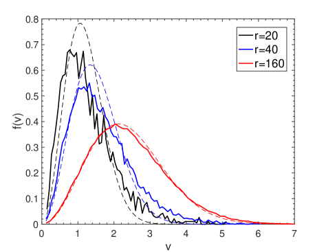
Figure 1: (a) 3D distribution of gas velocities $v_{t}$ (in numerical units) taken from an MHD turbulence simulation (Hu et al., 2021). (b) Turbulent speed distribution measured at different $r$’s (in the units of grids) in the MHD turbulence simulation. The dashed lines correspond to Eq. (2).

We note that due to different effects in star-forming regions, e.g., protostellar outflows, turbulent velocities may not always follow a power-law scaling (Hu et al., 2022). In addition, we will adopt a single turbulent scaling only down to $\sim 0.01~{}$ pc ($\sim 2000$ AU) as it may not apply on smaller scales due to the gravitational compression and gravity-driven turbulence (Xu & Lazarian, 2020; Guerrero-Gamboa & Vázquez-Semadeni, 2020). We also ignore the fact that turbulence in the presence of magnietic fields is typically anisotropic (Goldreich & Sridhar, 1995; Lazarian & Vishniac, 1999). The impact of these additional effects upon binary formation will be investigated in our future work.

3 Wide binaries with initial turbulent velocities

3.1 Formation of wide binaries

For a pair of stars to be gravitationally bound at birth, the relative velocity $v$ and $r$ must satisfy

$$v<{v_{\text{bon}}(r)\equiv}\sqrt{\frac{2GM}{r}},$$ (3)

where $M$ is the total mass of the binary. As an illustration, in Fig. 2 we present $v$ vs. $r$ for pairs of stars formed in turbulent gas over the range $0.01~{}\text{pc}<r<1$ pc (i.e., $2\times 10^{3}~{}\text{AU}<r<2\times 10^{5}$ AU). The colored region corresponds to $v<v_{\text{bon}}$ for $M=2M_{\odot}$. The color scale corresponds to $f(v)$ given by Eq. (2).

The intersection between $v_{\text{bon}}$ and $v_{\text{tur}}$ occurs at

$$r_{\text{int}}=\Big{(}\frac{2GML^{2\alpha}}{V_{L}^{2}}\Big{)}^{\frac{1}{2\alpha+1}},$$ (4)

which increases with increasing $M$ and $\alpha$. For instance, at $\alpha=1/3$ we have

$$r_{\text{int}}\approx 0.023~{}\text{pc}\Big{(}\frac{M}{M_{\odot}}\Big{)}^{0.6}\Big{(}\frac{L}{100~{}\text{pc}}\Big{)}^{0.4}\Big{(}\frac{V_{L}}{10~{}\text{km s}^{-1}}\Big{)}^{-1.2},$$ (5)

and at $\alpha=1/2$ we have

$$r_{\text{int}}\approx 0.093~{}\text{pc}\Big{(}\frac{M}{M_{\odot}}\Big{)}^{0.5}\Big{(}\frac{L}{100~{}\text{pc}}\Big{)}^{0.5}\Big{(}\frac{V_{L}}{10~{}\text{km s}^{-1}}\Big{)}^{-1}.$$ (6)

Obviously, at $r<r_{\text{int}}$ most pairs of stars can be gravitationally bound and form wide binaries. With the increase of $v_{\text{tur}}$ with $r$, at $r>r_{\text{int}}$, only a small fraction of pairs can form binaries.

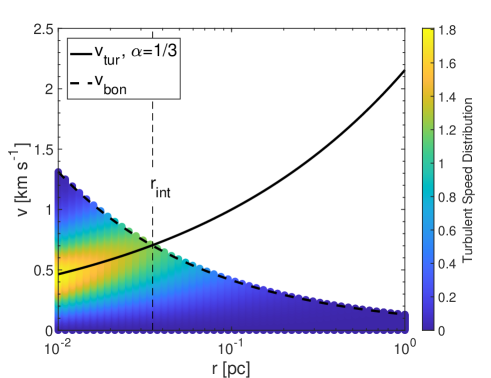
Figure 2: Initial velocity difference $v$ and separation $r$ between two stars formed in a turbulent environment. The colored region corresponds to a gravitationally bound system with $M=2M_{\odot}$. The color scale indicates the turbulent speed distribution (Eq. (2)). The thick dashed and solid lines correspond to $v_{\text{bon}}$ (Eq. (3)) and $v_{\text{tur}}$ (Eq. (1)), respectively. The vertical dashed line corresponds to $r_{\text{int}}$ (Eq. (4)). The parameters $V_{L}=10~{}\text{km}~{}\text{s}^{-1}$, $L=100~{}\text{pc}$, and $\alpha=1/3$ are used.

3.2 Eccentricity distribution

In this section we calculate the eccentricity distribution that results from random pairing of stars with relative velocities drawn from the distribution in Eq. (2).

For a bound two-body system, the specific energy and angular momentum are defined as

$$E=\frac{1}{2}v^{2}-\frac{GM}{r},~{}~{}\,\,\,\,\,\,\,J=rv\sin\theta,$$ (7)

where $\theta$ is the angle between the separation vector ${\bm{r}}$ and the relative velocity ${\bm{v}}$, and $E$ and $J$ are related to the eccentricity $e$ by

$$J^{2}=(1-e^{2})\frac{G^{2}M^{2}}{{(-2{E})}}.$$ (8)

Eliminating $E$ and $J$ from the above expressions leads to

$$\sin\theta=\frac{\sqrt{1-e^{2}}}{2u\sqrt{1-u^{2}}},{\rm~{}with~{}}u\equiv v/v_{\text{bon}}(r).$$ (9)

Note that $u\in(0,1)$ for bound binaries. The condition $\sin\theta\in(0,1)$ further constrains the range of $u$ as

$$\sqrt{\frac{1-e}{2}}<u<\sqrt{\frac{1+e}{2}}$$ (10)

at a given $e$.

Now we imagine that our random pairing process forms an ensemble of randomly oriented binaries of fixed $M$ at a given initial separation $r$. The resulting number density of these binaries in $(u,e)$ space satisfies (Eq. (9)),

$$dN \propto f(v)dvd\cos\theta$$ (11)

$$\propto\frac{f(u)du}{u\sqrt{1-u^{2}}\sqrt{e^{2}-(2u^{2}-1)^{2}}}ede,$$

where $f(u)$ is the distribution function of $u$. Therefore, we find the distribution function of $e$ at a given $r$ as

$${\color[rgb]{0,0,0}p(e)=C\,e\bigintssss_{\sqrt{(1-e)/2}}^{\sqrt{(1+e)/2}}\frac{f(u)du}{u\sqrt{1-u^{2}}\sqrt{e^{2}-(2u^{2}-1)^{2}}},}$$ (12)

where $C$ is a normalization constant, and the integral bounds are given by Eq. (10).

Obviously, $p(e)$ depends on the shape of $f(u)$ within the range of integration. As an illustration, Fig. 3 shows $p(e)$ (Eq. (12)) with $f(u)$ taking the form of Eq. (2) for various values of $\sigma_{u}=\sigma_{v}/v_{\text{bon}}$. When $\sigma_{u}$ is much less than unity, $p(e)$ has an excess (compared to the thermal distribution $p(e)=2e$) at large $e$’s and a deficiency at small $e$’s (see blue line in Fig. 3). The deficiency at small $e$’s is caused by the small $f(u)$ near $u=\sqrt{1/2}$ (corresponding to the circular orbit speed).

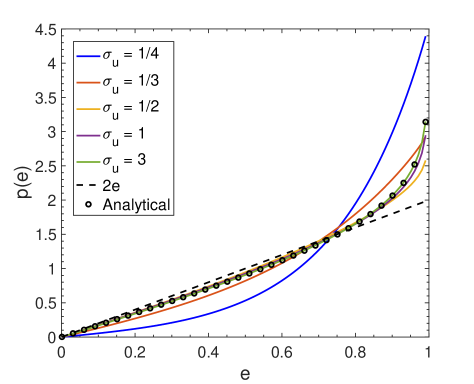
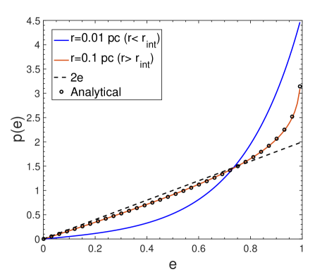
Figure 3: (a) $p(e)$ calculated using Eq. (12), where $f(u)$ takes the form in Eq. (2) with different values of $\sigma_{u}$ as labeled. The dashed line represents the thermal distribution ($p(e)=2e$). The circles correspond to the analytical estimate for $\sigma_{u}\gtrsim 1$ given by Eq. (13). (b) Same as (a) but with $\sigma_{u}=\sigma_{v}/v_{\text{bon}}(r)$ given by $\sigma_{v}=0.7v_{\text{tur}}$ and Eq. (1), using $M=2M_{\odot}$, $L=100$ pc, $V_{L}=10$ km s^-1, and $\alpha=1/3$. Two different values of $r$’s (as labeled) are considered, with $r<r_{\text{int}}$ and $r>r_{\text{int}}$ (see Eq. (4)) respectively.

When $\sigma_{u}$ is larger than unity, we approximately have $f(u)\propto u^{2}$ over $0<u<1$. In this case, Eq. (12) simplifies to

$$p(e) \approx\frac{1.06\,e}{\sqrt{1+e}}K\Bigg{(}\sqrt{\frac{2e}{1+e}}\Bigg{)},$$ (13)

where $K$ is the complete elliptic integral of the first kind (Gradshteyn & Ryzhik, 1994). As shown in Fig. 3, the above expression corresponds to a superthermal $p(e)$ and agrees well with the cases of large $\sigma_{u}$ (purple and green lines).

In Fig. 3, we present $p(e)$ (Eq. (12)) with $f(u)$ taking the form of Eq. (2) for $M=2M_{\odot}$, $L=100$ pc, $V_{L}=10$ km s^-1, and $\alpha=1/3$. At $r=0.01$ pc with $r<r_{\text{int}}$ (see Eqs. (5) and (6), Fig. 2), it falls in the regime where $\sigma_{u}$ is much less than unity. Therefore, we see a deficiency at small $e$’s and a significant excess at large $e$’s. At $r=0.1$ pc with $r>r_{\text{int}}$ and $\sigma_{u}$ larger than unity, the corresponding $p(e)$ is well described by Eq. (13) and is superthermal. We see that irrespective of the value of $\sigma_{u}$, a superthermal $p(e)$ is generally expected.

In Fig. 4, we compare our $p(e)$ of wide binaries taken from Fig. 3 and that of the wide binaries formed from dynamical unfolding of triple systems at $1$ Myr taken from Reipurth & Mikkola (2012). In the latter case, $p(e)$ for stable bound triples declines at large $e$’s. A superthermal $p(e)$ of the wide binaries at binary separations $>10^{3}$ AU in the Solar neighbourhood is indicated by Gaia observations (Hwang et al., 2022a) (see Fig. 4). Compared with the observations, we see a more significant excess at large $e$’s that we derive for young wide binaries. This excess is likely to be reduced by other physical processes that may occur after the binary formation, e.g. dynamical interaction/scatterings between binaries and passing stars and MCs. The superthermal $p(e)$ we find may therefore be important for understanding the observations, especially since those observations likely reflect the formation process of wide binaries rather than their subsequent dynamical interactions (Hamilton, 2022).

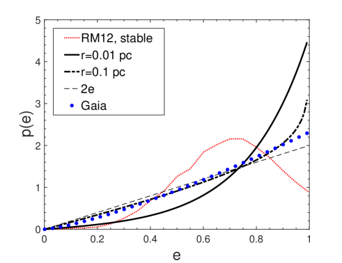
Figure 4: Comparison between $p(e)$ derived in this work (solid and dash-dotted lines, same as in Fig. 3) and that taken from Reipurth & Mikkola (2012) (RM12). Red dotted line represents the normalized $p(e)$ taken from Reipurth & Mikkola (2012) for the outer binaries in stable bound triples at $1$ Myr, with the distribution of semimajor axes of outer binaries peaked around $10^{3}$ AU. Dashed line is the thermal distribution. Blue circles show a power-law fit $p(e)\propto e^{1.32}$ to Gaia wide binaries with separations $10^{3.5}-10^{4}$ AU in the Galactic field (Hwang et al., 2022a).

4 Discussions

Observationally, wide binaries at separations $>10^{3}$ AU in the Solar neighbourhood have a superthermal eccentricity distribution (Hwang et al., 2022a). Since the effect of Galactic tides cannot produce the superthermal eccentricity distribution on its own and diffusive scattering with passing stars and MCs would tend to make the distribution more thermal (Hamilton, 2022), the observed eccentricity distribution is likely a relic of the wide binary formation mechanism.

Simulations show that wide binaries formed from cluster dissolution would have a thermal eccentricity distribution (Kouwenhoven et al., 2010) and therefore cannot explain the observation. While wide tertiaries formed from dynamical unfolding of compact triples are predicted to be highly eccentric (Reipurth & Mikkola, 2012), Hwang (2023) finds that the eccentricities of wide tertiaries in triples are similar to the wide binaries at the same separations, suggesting that the dynamical unfolding scenario plays a minor role. The remaining formation channels that form eccentric wide binaries are turbulent fragmentation (Bate et al., 1998) and random pairing during star formation phase (Tokovinin, 2017). Simulations of turbulent fragmentation suggest that wide binaries at $>10^{3}$ AU are eccentric ($e>0.6$) (Bate, 2014), although the number of binaries in simulations is too low to have well-characterized eccentricity distributions.

In this paper, we have focused on the eccentricity distribution that results from the random pairing scenario under the consideration that the initial relative velocities of pairs of stars are likely drawn from a characteristic turbulent velocity distribution of the star-forming gas. Given the typical turbulence conditions in star-forming regions, wide binaries formed from random pairing are expected to be highly eccentric, which may be (partly) responsible for the observed superthermal eccentricity.

We note that while the random pairing scenario may explain the high-eccentricity wide binaries, it is not clear whether it dominates the wide binary formation at $>10^{3}$ AU. Wide binaries formed from random pairing are weakly bound and their further gravitational interactions with other stars may disrupt the binaries. However, even if random pairing only contributes a few per cent of wide binaries at $>10^{3}$ AU, they may still significantly change the eccentricity distribution to superthermal (e.g. Hwang et al. 2022).

5 Summary

Turbulence plays a fundamental role in star formation. The turbulent motions in molecular gas are inherited by stars at their birth. Different from previous studies relying on the long-term dynamical evolution of stars and star clusters, we suggest that the formation of wide binaries with initial separations in the range $0.01~{}\text{pc}\lesssim r\lesssim 1$ pc (i.e., $2\times 10^{3}~{}\text{AU}\lesssim r\lesssim 2\times 10^{5}$ AU) is a natural consequence of star formation in the turbulent interstellar medium. With the velocity differences and separations of newly formed stars statistically following the turbulent velocity scaling, a pair of stars with a sufficiently small velocity difference at a given separation is gravitationally bound and can form a wide binary.

For a turbulent speed distribution of pairs of stars, we find that the resulting eccentricity distribution of the bound pairs is generally superthermal. This is true regardless of whether the average turbulent velocity $v_{\text{tur}}$ is smaller or larger than the escape velocity $v_{\text{bon}}$ of a gravitationally-bound binary. The superthermal $p(e)$ of wide binaries under this formation channel may be important for explaining the observed superthermal $p(e)$ in the Solar neighbourhood. Comparisons with future measurements on $p(e)$ in star-forming regions will provide testing of our theory.

References

- Allen et al. (2007) Allen, C., Poveda, A., & Hernández-Alcántara, A. 2007, in Binary Stars as Critical Tools & Tests in Contemporary Astrophysics, ed. W. I. Hartkopf, P. Harmanec, & E. F. Guinan, Vol. 240, 405–413, doi: 10.1017/S174392130700436X
- Andrews et al. (2019) Andrews, J. J., Anguiano, B., Chanamé, J., et al. 2019, ApJ, 871, 42, doi: 10.3847/1538-4357/aaf502
- Armstrong et al. (1995) Armstrong, J. W., Rickett, B. J., & Spangler, S. R. 1995, ApJ, 443, 209, doi: 10.1086/175515
- Bahcall et al. (1985) Bahcall, J. N., Hut, P., & Tremaine, S. 1985, ApJ, 290, 15, doi: 10.1086/162953
- Bate (2014) Bate, M. R. 2014, MNRAS, 442, 285, doi: 10.1093/mnras/stu795
- Bate et al. (1998) Bate, M. R., Clarke, C. J., & McCaughrean, M. J. 1998, MNRAS, 297, 1163, doi: 10.1046/j.1365-8711.1998.01565.x
- Burkhart (2021) Burkhart, B. 2021, PASP, 133, 102001, doi: 10.1088/1538-3873/ac25cf
- Chamandy & Shukurov (2020) Chamandy, L., & Shukurov, A. 2020, Galaxies, 8, 56, doi: 10.3390/galaxies8030056
- Chanamé & Gould (2004) Chanamé, J., & Gould, A. 2004, ApJ, 601, 289, doi: 10.1086/380442
- Chepurnov & Lazarian (2010) Chepurnov, A., & Lazarian, A. 2010, ApJ, 710, 853, doi: 10.1088/0004-637X/710/1/853
- Cho & Lazarian (2002) Cho, J., & Lazarian, A. 2002, Physical Review Letters, 88, 245001, doi: 10.1103/PhysRevLett.88.245001
- Deacon & Kraus (2020) Deacon, N. R., & Kraus, A. L. 2020, MNRAS, 496, 5176, doi: 10.1093/mnras/staa1877
- El-Badry & Rix (2018) El-Badry, K., & Rix, H.-W. 2018, MNRAS, 480, 4884, doi: 10.1093/mnras/sty2186
- El-Badry et al. (2021) El-Badry, K., Rix, H.-W., & Heintz, T. M. 2021, MNRAS, 506, 2269, doi: 10.1093/mnras/stab323
- Elmegreen & Scalo (2004) Elmegreen, B. G., & Scalo, J. 2004, ARA&A, 42, 211, doi: 10.1146/annurev.astro.41.011802.094859
- Federrath et al. (2011) Federrath, C., Chabrier, G., Schober, J., et al. 2011, Physical Review Letters, 107, 114504, doi: 10.1103/PhysRevLett.107.114504
- Federrath et al. (2009) Federrath, C., Klessen, R. S., & Schmidt, W. 2009, ApJ, 692, 364, doi: 10.1088/0004-637X/692/1/364
- Gaia Collaboration et al. (2016) Gaia Collaboration, Brown, A. G. A., Vallenari, A., et al. 2016, A&A, 595, A2, doi: 10.1051/0004-6361/201629512
- Gaia Collaboration et al. (2019) Gaia Collaboration, Eyer, L., Rimoldini, L., et al. 2019, A&A, 623, A110, doi: 10.1051/0004-6361/201833304
- Goldreich & Sridhar (1995) Goldreich, P., & Sridhar, S. 1995, ApJ, 438, 763, doi: 10.1086/175121
- Gradshteyn & Ryzhik (1994) Gradshteyn, I. S., & Ryzhik, I. M. 1994, Table of integrals, series and products
- Guerrero-Gamboa & Vázquez-Semadeni (2020) Guerrero-Gamboa, R., & Vázquez-Semadeni, E. 2020, ApJ, 903, 136, doi: 10.3847/1538-4357/abba1f
- Ha et al. (2022) Ha, T., Li, Y., Kounkel, M., et al. 2022, ApJ, 934, 7, doi: 10.3847/1538-4357/ac76bf
- Ha et al. (2021) Ha, T., Li, Y., Xu, S., Kounkel, M., & Li, H. 2021, ApJ, 907, L40, doi: 10.3847/2041-8213/abd8c9
- Hamilton (2022) Hamilton, C. 2022, The Astrophysical Journal Letters, 929, L29
- Hartman & Lépine (2020) Hartman, Z. D., & Lépine, S. 2020, ApJS, 247, 66, doi: 10.3847/1538-4365/ab79a6
- Hawkins et al. (2020) Hawkins, K., Lucey, M., Ting, Y.-S., et al. 2020, MNRAS, 492, 1164, doi: 10.1093/mnras/stz3132
- Hennebelle & Falgarone (2012) Hennebelle, P., & Falgarone, E. 2012, A&A Rev., 20, 55, doi: 10.1007/s00159-012-0055-y
- Heyer & Brunt (2004) Heyer, M. H., & Brunt, C. M. 2004, ApJ, 615, L45, doi: 10.1086/425978
- Hu et al. (2022) Hu, Y., Federrath, C., Xu, S., & Mathew, S. S. 2022, MNRAS, 513, 2100, doi: 10.1093/mnras/stac972
- Hu et al. (2021) Hu, Y., Xu, S., & Lazarian, A. 2021, ApJ, 911, 37, doi: 10.3847/1538-4357/abea18
- Hwang (2023) Hwang, H.-C. 2023, MNRAS, 518, 1750, doi: 10.1093/mnras/stac3116
- Hwang et al. (2022) Hwang, H.-C., El-Badry, K., Rix, H.-W., et al. 2022, ApJ, 933, L32, doi: 10.3847/2041-8213/ac7c70
- Hwang et al. (2020) Hwang, H.-C., Hamer, J. H., Zakamska, N. L., & Schlaufman, K. C. 2020, MNRAS, 497, 2250, doi: 10.1093/mnras/staa2124
- Hwang et al. (2021) Hwang, H.-C., Ting, Y.-S., Schlaufman, K. C., Zakamska, N. L., & Wyse, R. F. G. 2021, MNRAS, 501, 4329, doi: 10.1093/mnras/staa3854
- Hwang et al. (2022a) Hwang, H.-C., Ting, Y.-S., & Zakamska, N. L. 2022a, Monthly Notices of the Royal Astronomical Society, 512, 3383
- Hwang et al. (2022b) Hwang, H.-C., Ting, Y.-S., Conroy, C., et al. 2022b, Monthly Notices of the Royal Astronomical Society, 513, 754
- Igoshev & Perets (2019) Igoshev, A. P., & Perets, H. B. 2019, MNRAS, 486, 4098, doi: 10.1093/mnras/stz1024
- Inoue et al. (2018) Inoue, T., Hennebelle, P., Fukui, Y., et al. 2018, PASJ, 70, S53, doi: 10.1093/pasj/psx089
- Kouwenhoven et al. (2010) Kouwenhoven, M. B. N., Goodwin, S. P., Parker, R. J., et al. 2010, in Astronomical Society of the Pacific Conference Series, Vol. 435, Binaries - Key to Comprehension of the Universe, ed. A. Prša & M. Zejda, 165. https://arxiv.org/abs/0909.1225
- Kowal & Lazarian (2010) Kowal, G., & Lazarian, A. 2010, ApJ, 720, 742, doi: 10.1088/0004-637X/720/1/742
- Kritsuk et al. (2017) Kritsuk, A. G., Ustyugov, S. D., & Norman, M. L. 2017, New Journal of Physics, 19, 065003, doi: 10.1088/1367-2630/aa7156
- Krolikowski et al. (2021) Krolikowski, D. M., Kraus, A. L., & Rizzuto, A. C. 2021, AJ, 162, 110, doi: 10.3847/1538-3881/ac0632
- Kroupa & Burkert (2001) Kroupa, P., & Burkert, A. 2001, ApJ, 555, 945, doi: 10.1086/321515
- Lazarian (2009) Lazarian, A. 2009, Space Science Reviews, 143, 357, doi: 10.1007/s11214-008-9460-y
- Lazarian & Pogosyan (2000) Lazarian, A., & Pogosyan, D. 2000, ApJ, 537, 720, doi: 10.1086/309040
- Lazarian & Pogosyan (2006) —. 2006, ApJ, 652, 1348, doi: 10.1086/508012
- Lazarian & Vishniac (1999) Lazarian, A., & Vishniac, E. T. 1999, ApJ, 517, 700, doi: 10.1086/307233
- Lazarian et al. (2018) Lazarian, A., Yuen, K. H., Ho, K. W., et al. 2018, ApJ, 865, 46, doi: 10.3847/1538-4357/aad7ff
- Livernois et al. (2023) Livernois, A. R., Vesperini, E., & Pavlík, V. 2023, arXiv e-prints, arXiv:2303.12841, doi: 10.48550/arXiv.2303.12841
- Mac Low & Klessen (2004) Mac Low, M.-M., & Klessen, R. S. 2004, Reviews of Modern Physics, 76, 125, doi: 10.1103/RevModPhys.76.125
- MATLAB (2021) MATLAB. 2021, MATLAB and Statistics Toolbox Release 2021b (Natick, Massachusetts: The MathWorks Inc.)
- McKee & Ostriker (2007) McKee, C. F., & Ostriker, E. C. 2007, ARA&A, 45, 565, doi: 10.1146/annurev.astro.45.051806.110602
- Mocz & Burkhart (2018) Mocz, P., & Burkhart, B. 2018, MNRAS, 480, 3916, doi: 10.1093/mnras/sty1976
- Moeckel & Clarke (2011) Moeckel, N., & Clarke, C. J. 2011, MNRAS, 415, 1179, doi: 10.1111/j.1365-2966.2011.18731.x
- Monroy-Rodríguez & Allen (2014) Monroy-Rodríguez, M. A., & Allen, C. 2014, ApJ, 790, 159, doi: 10.1088/0004-637X/790/2/159
- Padoan et al. (2016) Padoan, P., Pan, L., Haugbølle, T., & Nordlund, Å. 2016, ApJ, 822, 11, doi: 10.3847/0004-637X/822/1/11
- Peñarrubia (2021) Peñarrubia, J. 2021, MNRAS, 501, 3670, doi: 10.1093/mnras/staa3700
- Peñarrubia et al. (2016) Peñarrubia, J., Ludlow, A. D., Chanamé, J., & Walker, M. G. 2016, MNRAS, 461, L72, doi: 10.1093/mnrasl/slw090
- Qian et al. (2018) Qian, L., Li, D., Gao, Y., Xu, H., & Pan, Z. 2018, ApJ, 864, 116, doi: 10.3847/1538-4357/aad780
- Quinn et al. (2009) Quinn, D. P., Wilkinson, M. I., Irwin, M. J., et al. 2009, MNRAS, 396, L11, doi: 10.1111/j.1745-3933.2009.00652.x
- Rani et al. (2022) Rani, R., Moore, T. J. T., Eden, D. J., & Rigby, A. J. 2022, MNRAS, 515, 271, doi: 10.1093/mnras/stac1812
- Reipurth & Mikkola (2012) Reipurth, B., & Mikkola, S. 2012, Nature, 492, 221, doi: 10.1038/nature11662
- Stone et al. (1998) Stone, J. M., Ostriker, E. C., & Gammie, C. F. 1998, ApJ, 508, L99, doi: 10.1086/311718
- Tian et al. (2020) Tian, H.-J., El-Badry, K., Rix, H.-W., & Gould, A. 2020, ApJS, 246, 4, doi: 10.3847/1538-4365/ab54c4
- Tokovinin (2017) Tokovinin, A. 2017, MNRAS, 468, 3461, doi: 10.1093/mnras/stx707
- Tokovinin (2020) —. 2020, MNRAS, 496, 987, doi: 10.1093/mnras/staa1639
- Volgenau (2004) Volgenau, N. H. 2004, PhD thesis, University of Maryland, llege Park, Maryland, USA
- Ward-Thompson et al. (2007) Ward-Thompson, D., André, P., Crutcher, R., et al. 2007, in Protostars and Planets V, ed. B. Reipurth, D. Jewitt, & K. Keil, 33. https://arxiv.org/abs/astro-ph/0603474
- Xu (2020) Xu, S. 2020, MNRAS, 492, 1044, doi: 10.1093/mnras/stz3092
- Xu & Hu (2021) Xu, S., & Hu, Y. 2021, ApJ, 910, 88, doi: 10.3847/1538-4357/abe403
- Xu et al. (2019) Xu, S., Ji, S., & Lazarian, A. 2019, ApJ, 878, 157, doi: 10.3847/1538-4357/ab21be
- Xu & Lazarian (2020) Xu, S., & Lazarian, A. 2020, ApJ, 890, 157, doi: 10.3847/1538-4357/ab6e63
- Xu & Zhang (2017) Xu, S., & Zhang, B. 2017, ApJ, 835, 2, doi: 10.3847/1538-4357/835/1/2
- Xu & Zhang (2020) —. 2020, ApJ, 905, 159, doi: 10.3847/1538-4357/abc69f
- Yuen et al. (2022) Yuen, K. H., Ho, K. W., Law, C. Y., Chen, A., & Lazarian, A. 2022, arXiv e-prints, arXiv:2204.13760. https://arxiv.org/abs/2204.13760
- Zhou et al. (2021) Zhou, J.-X., Li, G.-X., & Chen, B.-Q. 2021, arXiv:2110.11595, arXiv:2110.11595. https://arxiv.org/abs/2110.11595