Topological phase diagrams of in-plane field polarized Kitaev magnets

Abstract

While the existence of a magnetic field induced quantum spin liquid in Kitaev magnets remains under debate, its topological properties often extend to proximal phases where they can lead to unusual behaviors of both fundamental and applied interests. Subjecting a generic nearest neighbor spin model of Kitaev magnets to a sufficiently strong in-plane magnetic field, we study the resulting polarized phase and the associated magnon excitations. In contrast to the case of an out-of-plane magnetic field where the magnon band topology is enforced by a three-fold symmetry, we find that it is possible for topologically trivial and nontrivial parameter regimes to coexist under in-plane magnetic fields. We map out the topological phase diagrams of the magnon bands, revealing a rich pattern of variation of the Chern number over the parameter space and the field angle. We further compute the magnon thermal Hall conductivity as a weighted summation of Berry curvatures, and discuss experimental implications of our results to planar thermal Hall effects in Kitaev magnets.

Introduction.—Kitaev spin liquid (KSL) is the ground state of an exactly soluble spin model on a honeycomb lattice with bond dependent Ising interactions [1]. It features Majorana fermions and $\mathbb{Z}_{2}$ gauge fields, both of which originate from fractionalizations of $S=1/2$ degrees of freedom. Without an external magnetic field, the spectrum of Majorana fermions is gapless at the $\mathrm{K}$ and $\mathrm{K}^{\prime}$ points, forming conic singularities similar to Dirac cones in the electronic dispersion of graphene. By applying a perturbative field $\mathbf{h}=(h_{x},h_{y},h_{z})$, the spectrum acquires a gap $\Delta\sim\lvert h_{x}h_{y}h_{z}\rvert/K^{2}$, and the lower band a Chern number $\nu=\mathrm{sgn}(h_{x}h_{y}h_{z})$, see Figs. 1a and 1b. The resulting non-Abelian KSL is predicted to exhibit a half quantized thermal Hall conductivity $\kappa_{xy}^{\mathrm{2D}}/T=(\nu/2)(\pi k_{\mathrm{B}}^{2}/6\hbar)$ due to chiral Majorana edge modes .

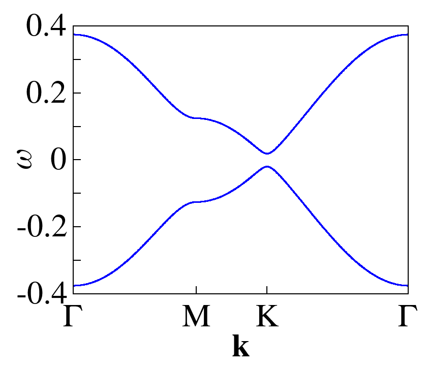
(a)

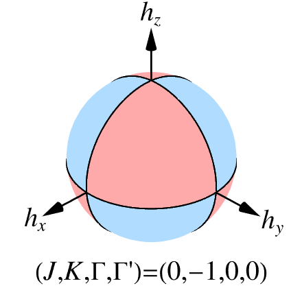
(b)

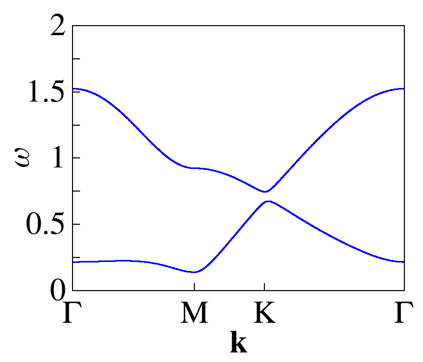
(c)

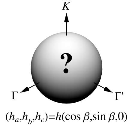
(d)

Figure 1: (a) Majorana spectrum of the ferromagnetic Kitaev model subjected to a perturbative magnetic field, with $K=-1$ and $\lvert h_{x}h_{y}h_{z}/K^{3}\rvert\sim 0.01$. (b) For the non-Abelian Kitaev spin liquid, the Chern number of the lower Majorana band depends on the field direction through $\nu=\mathrm{sgn}(h_{x}h_{y}h_{z})$. Red (blue) areas indicate $\nu=+1$ ($-1$), while black curves indicate the vanishing of the band gap. (c) Magnon spectrum of the polarized state in a realistic nearest neighbor spin model (1) of the Kitaev magnet $\alpha$-RuCl₃ under an in-plane magnetic field along the $a$ axis, with $(J,K,\Gamma,\Gamma^{\prime})=(-1/8,-1,+1/2,-1/8)$ and $h=0.2$. The lower (upper) magnon band carries Chern number $+1$ ($-1$). (d) For the polarized state under an in-plane magnetic field, we find nontrivial patterns traced out by the variation of the magnon Chern number over the space of couplings and the field angle, see Figs. 3a-3f.

In recent years, there have been tremendous efforts in the search for KSL in candidate materials, ranging from iridates [3, 4, 5] to ruthenium halides [6, 7, 8] to cobaltates [9, 10]. These so called Kitaev magnets [11, 12, 13, 14], which have partially filled $d$ orbitals and a significant spin orbit coupling, may realize a dominant Kitaev interaction $K$ via Jackeli-Khaliullin [15] or related [16, 17, 18] mechanism. Here, we focus on arguably the most popular amongst them, $\alpha$-RuCl₃ [19]. Like most Kitaev magnets, the zero field ground state of $\alpha$-RuCl₃ is a zigzag (ZZ) magnetic order [20, 21], due to the presence of other symmetry allowed interactions than $K$ [22]. However, an external magnetic field is found to suppress the ZZ order and promote a disordered phase, which may be the non-Abelian KSL, as evidenced by the half integer thermal Hall effect reported in Refs. [23, 24, 25, 26, 27]. Since the field-temperature window of the half quantization is rather small, it is suggested that the field angle dependence of thermal Hall conductivity [25] or heat capacity [28, 29] can lend further support for the case of non-Abelian KSL. Meanwhile, other experiments [30, 31] report that the thermal Hall conductivity in the field induced phase behaves rather like a smooth function without any plateau, and it decreases rapidly as the temperature approaches zero, which suggest emergent heat carriers of a bosonic nature.

While the existence of KSL at intermediate fields remains under debate [32, 33, 34, 35, 36, 37, 38, 39], Kitaev magnets eventually polarize at sufficiently high fields. In this case, the collective excitations are magnons, which can give rise to experimentally measurable transport signals at finite temperatures. Furthermore, if the magnon bands are topological, the resulting thermal Hall conductivity can reach the same order of magnitude as the half quantized value [40, 41, 42, 43]. Although for magnons $\kappa_{xy}$ at low temperatures is not directly proportional to $\nu$ (the Chern number of the lower band), the latter is very often a good indicator of the opposite sign of the former. Therefore, phase diagrams that reveal the magnon Chern number across generic model parameters of Kitaev magnets [44] will be valuable for identifying topological magnons and interpreting thermal transport measurements at high fields, see Figs. 1c and 1d. The main objective of this Letter is precisely to present such topological phase diagrams for in-plane magnetic fields, which are relevant to experiments of planar thermal Hall effect [25, 26, 30, 31, 45].

We note that Kitaev magnets such as $\alpha$-RuCl₃ reaches the polarized state more easily under in-plane fields than an out-of-plane field, likely due to an anisotropic $g$ tensor [46, 47, 48, 49] and a positive $\Gamma$ interaction [50], which discounts the out-of-plane field strength and disfavors an out-of-plane magnetization, respectively [41, 51]. Also, the case of subjecting Kitaev magnets with nearest neighbor interactions to strong out-of-plane fields, which preserve the $C_{3}$ symmetry, has been studied in the pioneering work Ref. [52] (see also Ref. [53]). It is found that, for the linear spin wave theory of the polarized state, $\Gamma$ and $\Gamma^{\prime}$ can be absorbed into $J$, $K$, and $h$, which effectively reduces the $JK\Gamma\Gamma^{\prime}$ model to a $JK$ model and greatly simplifies the problem. The $C_{3}$ symmetry also plays an important role in the diagnosis of magnon band topology based on topological quantum chemistry [54, 55], where one examines if the elementary band representation splits into disconnected bands. As demonstrated in Ref. [56], the magnon bands must be topological whenever a gap exists in between, which is consistent with the results from explicit calculations [52]. These make the out-of-plane field rather special.

In this Letter, we consider the nearest neighbor $JK\Gamma\Gamma^{\prime}$ model under sufficiently high in-plane magnetic fields, such that the corresponding polarized states are stable. Unlike the case of an out-of-plane field, the model has to be taken in full as none of the parameters can be made redundant. To map out the phase diagrams of topological magnons, we first solve analytically for the parameter regions where the gap between the two bands closes, which are potential phase boundaries for topological transitions, at generic in-plane field directions. For ease of visualizations, we then set $J=0$, compute the Chern number $\nu$ where it is well defined, and plot the results at several field angles. As long as the field is not along the armchair direction, we always find parameter regions that are topological ($\nu=\pm 1$) as well as those that are trivial ($\nu=0$). If instead the field is along the armchair direction, then all gapped parameter regions are topologically trivial due to a $C_{2}$ symmetry [40]. Rotating the field in the honeycomb plane, we find that the total area of parameter regions with topological magnons is the largest when the field is along the zigzag direction. We also provide an understanding as to why certain parameter regions are topologically trivial, via an effective Hamiltonian at high fields [52]. Finally, we discuss the implications of our results to thermal Hall conductivities and model parameters of Kitaev magnets, which will provide helpful guidances to related experiments. Detailed calculations are presented in Supplemental Material [57].

Linear spin wave theory.—The most generic nearest neighbor spin model of Kitaev magnets is the $JK\Gamma\Gamma^{\prime}$ model [22]. In an external magnetic field $\mathbf{h}$, it reads

$$H= \sum_{\lambda=x,y,z}\sum_{\langle ij\rangle\in\lambda}\big{[}J\mathbf{S}_{i}\cdot\mathbf{S}_{j}+KS_{i}^{\lambda}S_{j}^{\lambda}+\Gamma(S_{i}^{\mu}S_{j}^{\nu}+S_{i}^{\nu}S_{j}^{\mu})$$ (1)

$$+\Gamma^{\prime}(S_{i}^{\mu}S_{j}^{\lambda}+S_{i}^{\lambda}S_{j}^{\mu}+S_{i}^{\nu}S_{j}^{\lambda}+S_{i}^{\lambda}S_{j}^{\nu})\big{]}-\sum_{i}\mathbf{h}\cdot\mathbf{S}_{i},$$

where $(\lambda,\mu,\nu)$ is a cyclic permutation of $(x,y,z)$. For convenience of analysis, we measure the field strength $\lvert\mathbf{h}\rvert\equiv hS$ in portions of the spin magnitude $S\equiv\lvert\mathbf{S}_{i}\rvert$. We also take $S$ to be dimensionless so that $J,K,\Gamma,\Gamma^{\prime}$ and $h$ have units of energy. An in-plane field can be parametrized as $(h_{a},h_{b},h_{c})=h(\cos\beta,\sin\beta,0)$, where $\beta\in[0,2\pi)$ is the azimuthal angle in the honeycomb plane, with $\beta=0$ ($\pi/2$) corresponding to the $a$ ($b$) direction , see Fig. 2a. We apply the linear spin wave theory [59, 60] to the in-plane field polarized state of (1), and obtain an analytical expression of the magnon spectrum $\omega_{\pm}(\mathbf{k})=S\sqrt{E(\mathbf{k})\pm\Delta(\mathbf{k})}/2$, where

$$E(\mathbf{k})=4(h-c_{1})^{2}+\big{\lvert}c_{2}f_{\mathbf{k}}+c_{4}g_{\mathbf{k}}\big{\rvert}^{2}-\big{\lvert}c_{5}f_{\mathbf{k}}-c_{4}g_{\mathbf{k}}\big{\rvert}^{2}-4\big{\lvert}c_{6}(f_{\mathbf{k}}-3)+c_{7}g_{\mathbf{k}}\big{\rvert}^{2}+c_{3}(c_{2}+c_{5})(f_{\mathbf{k}}+f_{\mathbf{k}}^{*}),$$ (2a)

$$\begin{split}&\Delta^{2}(\mathbf{k})=16(h-c_{1})^{2}\big{\lvert}c_{2}f_{\mathbf{k}}+c_{3}+c_{4}g_{\mathbf{k}}\big{\rvert}^{2}+(c_{2}+c_{5})\Big{\{}(c_{2}+c_{5})\big{[}f_{\mathbf{k}}(c_{3}+c_{4}g_{\mathbf{k}}^{*})-f_{\mathbf{k}}^{*}(c_{3}+c_{4}g_{\mathbf{k}})\big{]}^{2}\\ &\qquad\quad\;\>+8\big{[}f_{\mathbf{k}}(3c_{6}-c_{7}g_{\mathbf{k}}^{*})-f_{\mathbf{k}}^{*}(3c_{6}-c_{7}g_{\mathbf{k}})\big{]}\big{[}c_{6}f_{\mathbf{k}}(c_{3}+c_{4}g_{\mathbf{k}}^{*})-c_{6}f_{\mathbf{k}}^{*}(c_{3}+c_{4}g_{\mathbf{k}})+(g_{\mathbf{k}}-g_{\mathbf{k}}^{*})(c_{3}c_{7}+3c_{4}c_{6})\big{]}\\ &\qquad\quad\;\>+4(c_{2}-c_{5})\big{[}f_{\mathbf{k}}(3c_{6}-c_{7}g_{\mathbf{k}}^{*})-f_{\mathbf{k}}^{*}(3c_{6}-c_{7}g_{\mathbf{k}})\big{]}^{2}\Big{\}},\end{split}$$ (2b)

$$\begin{split}&c_{1}=3J+K-\Gamma-2\Gamma^{\prime},c_{2}=\frac{1}{6}\left[12J+4K+2\Gamma+4\Gamma^{\prime}+(K+2\Gamma-2\Gamma^{\prime})\cos(2\beta)\right],c_{3}=-\frac{\cos(2\beta)}{2}\left(K+2\Gamma-2\Gamma^{\prime}\right),\\ &c_{4}=\frac{\sin(2\beta)}{2\sqrt{3}}\left(K+2\Gamma-2\Gamma^{\prime}\right),c_{5}=\Gamma+2\Gamma^{\prime}-\frac{\cos(2\beta)}{6}\left(K+2\Gamma-2\Gamma^{\prime}\right),c_{6}=\frac{\sin\beta}{3\sqrt{2}}\left(K-\Gamma+\Gamma^{\prime}\right),c_{7}=\frac{\cos\beta}{\sqrt{6}}\left(K-\Gamma+\Gamma^{\prime}\right),\end{split}$$ (2c)

$f_{\mathbf{k}}=1+\exp(ik_{1})+\exp(ik_{2})$, $g_{\mathbf{k}}=\exp(ik_{1})-\exp(ik_{2})$, and $k_{1},k_{2}\in[0,2\pi)$ are components of the crystal momentum defined according to $\mathbf{a}_{1}$ and $\mathbf{a}_{2}$ in Fig. 2a . Let $\Delta(\mathbf{k})=\sqrt{\Delta^{2}(\mathbf{k})}\geq 0$, so that $\omega_{-}(\mathbf{k})$ [$\omega_{+}(\mathbf{k})$] corresponds to the lower (upper) band. As a clarification, we refer to the gap between the upper and lower bands, $\min_{\mathbf{k}}[\omega_{+}(\mathbf{k})-\omega_{-}(\mathbf{k})]\geq 0$, as the band gap, which is not to be confused with the excitation gap, $\min_{\mathbf{k}}\omega_{-}(\mathbf{k})>0$. Chern number is a topological invariant that can never change as long as a finite band gap is maintained [62], i.e., a topological phase transition can only occur when the band gap vanishes, which happens if and only if $\Delta(\mathbf{k})=0$ for some $\mathbf{k}=\mathbf{k}_{*}$.

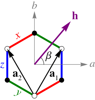
(a)

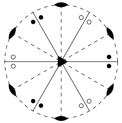
(b)

Figure 2: (a) The three types of nearest neighbor bonds, $x$, $y$, and $z$, of Kitaev magnets are indicated by red, green, and blue colors, respectively. The in-plane crystallographic axes $a$ and $b$ are along the zigzag and armchair directions, respectively. The out-of-plane $c$ axis is not shown here. An external magnetic field $\mathbf{h}$ is applied in-plane at the azimuthal angle $\beta$. The choices of primitive lattice vectors $\mathbf{a}_{1}$ and $\mathbf{a}_{2}$ are also indicated. (b) The point group of the $JK\Gamma\Gamma^{\prime}$ model is $\bar{3}m$ or $D_{3d}$. This diagram also represents how the magnon Chern number $\nu$ changes as $\mathbf{h}$ transforms under elements of $\bar{3}m$ and time reversal $\mathcal{T}$. If a filled circle is mapped to an empty circle or vice versa, then $\nu$ flips sign. If a circle is mapped to another circle of the same type, then $\nu$ remains invariant. Due to symmetry, it is sufficient to study field angles in the range $0\leq\beta\leq\pi/6$.

Table 1: For field angles $\beta\neq\pi/6\,(\mathrm{mod}\,\pi/3)$, the band gap closes if the parameters of the $JK\Gamma\Gamma^{\prime}$ model satisfy any of the following equations. They define the phase boundaries of topological transitions. For field angles $\beta=\pi/6\,(\mathrm{mod}\,\pi/3)$, the band gap is zero whenever (I) or (4) is satisfied.

I	$K+2\Gamma-2\Gamma^{\prime}=0$
II	$6J+2K+\Gamma+2\Gamma^{\prime}=0$
III	$6J+2K+\Gamma+2\Gamma^{\prime}+2(K+2\Gamma-2\Gamma^{\prime})\cos(2\beta)=0$
IV	$6J+2K+\Gamma+2\Gamma^{\prime}-2(K+2\Gamma-2\Gamma^{\prime})\cos(2\beta+\pi/3)=0$
V	$6J+2K+\Gamma+2\Gamma^{\prime}-2(K+2\Gamma-2\Gamma^{\prime})\cos(2\beta-\pi/3)=0$
VI	$3J+K+2\Gamma+4\Gamma^{\prime}=0$   if (4) holds
VII	$K-\Gamma+\Gamma^{\prime}=0$   if (4) holds

We assume a stable polarized state, where the excitation gap increases with $h$, so that the system becomes more stable as $h$ grows, rather than undergoing a magnon instability where the excitation gap goes to zero. As demonstrated in Supplemental Material [57], this requires $h>c_{1}$, from which we deduce the following. For a given set of parameters $\{J,K,\Gamma,\Gamma^{\prime}\}$, (i) if the band gap is zero, then it remains zero as $h$ varies, and (ii) if the band gap is finite, then it remains finite as $h$ varies, unless $h\longrightarrow\infty$ while the couplings stay finite. These imply that the topological phase diagrams are independent of the field strength, and, for a given field angle, we can map them out by first solving for the zeros of (LABEL:Dksquaredefine), which define the boundaries, then choose a sufficiently high field to compute the Chern numbers [63, 64, 65, 66] for the parameters away from these zeros.

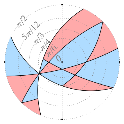
(a)

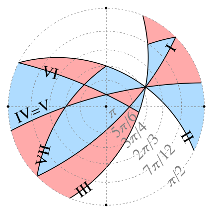
(b)

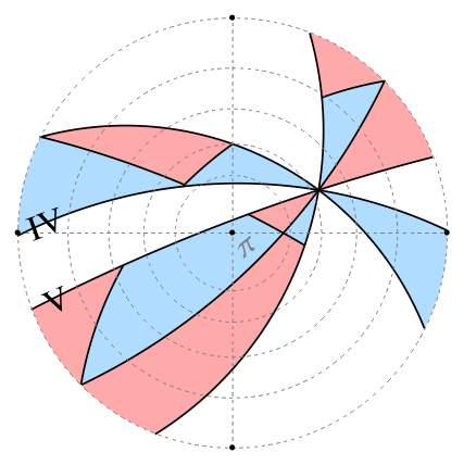
(c)

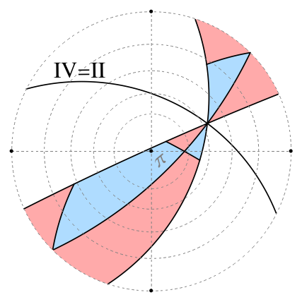
(d)

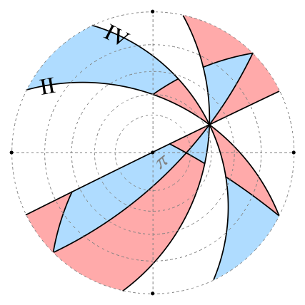
(e)

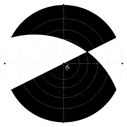
(f)

Figure 3: Topological phase diagrams, which indicate the Chern number $\nu$ of the lower magnon band, of the in-plane field polarized states, over the space of couplings parametrized by $(J,K,\Gamma,\Gamma^{\prime})=(0,\cos\theta,\sin\theta\cos\phi,\sin\theta\sin\phi)$, at field angles $\beta$ equal to (a,b) $0$, (c) $\pi/24$, (d) $\pi/12$, (e) $\pi/8$, and (f) $\pi/6$. Red, white, and blue areas indicate $\nu=+1$, $0$, and $-1$, respectively, while black curves or areas indicate the vanishing of the band gap. The latter defines the phase boundaries, which are labeled by roman numerals as in Table 1. Grey dashed lines indicate latitudes at selected zenith angles $\theta$. In each diagram, the center is either the $K>0$ ($\theta=0$) limit, as in (a), or the $K<0$ ($\theta=\pi$) limit, as in (b-f), while the left, right, top, and bottom ends on the equator $\theta=\pi/2$ are the $\Gamma>0$ ($\phi=0$), $\Gamma<0$ ($\phi=\pi$), $\Gamma^{\prime}>0$ ($\phi=\pi/2$), and $\Gamma^{\prime}<0$ ($\phi=3\pi/2$) limits, respectively.

Topological phase diagrams.—At finite in-plane fields, the band gap closes if and only if the set of parameters $\{J,K,\Gamma,\Gamma^{\prime}\}$ meets any of the criteria listed in Table 1. For parameters with a finite band gap, let the Chern number of the lower (upper) band be $\nu$ ($-\nu$). From the symmetries of the $JK\Gamma\Gamma^{\prime}$ model, one can relate the phase diagrams at different field angles by the following rules [57]. Fixing the couplings, (i) $\nu\longrightarrow\nu$ if $\mathbf{h}$ is rotated by $2\pi/3$ about the $c$ axis, (ii) $\nu\longrightarrow-\nu$ if $\mathbf{h}$ is rotated by $\pi$ about the $b$ axis, and (iii) $\nu\longrightarrow-\nu$ if $\mathbf{h}\longrightarrow-\mathbf{h}$ is reversed [41], while the phase boundaries are invariant under each of these actions. In other words, the Chern number transforms according to the $A_{2g}$ representation of the point group $\bar{3}m$ [67, 68], and flips sign under time reversal $\mathcal{T}$, as in the case of non-Abelian KSL [28]. Hence, $\beta\in[0,\pi/6]$ serves as an independent unit, to which all other angles can be related by symmetries, see Fig. 2b. On the other hand, flipping the signs of all couplings leaves the Chern number invariant [57].

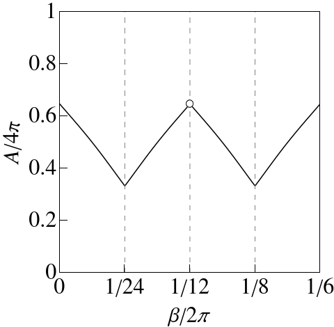
Figure 4: The total area $A$ of parameter regions with topological magnons on the $K\Gamma\Gamma^{\prime}$ sphere, as a function of the field angle $\beta$, over the range $0\leq\beta\leq\pi/3$. There is a discontinuity at $\beta=\pi/6$ (indicated by the empty circle) as $A=0$ is enforced by a $C_{2}$ symmetry, while large swathes of the parameter space become critical, see Fig. 3f.

For visualizations, we set $J=0$, and calculate $\nu$ over the spherical parameter space defined by $K^{2}+\Gamma^{2}+{\Gamma^{\prime}}^{2}=1$, at the field angles $\beta=0,\pi/24,\pi/12,\pi/8,\pi/6$. The results are plotted in Figs. 3a-3f, mainly on the hemisphere with $K<0$ relevant to Kitaev magnets, while that with $K>0$ can be related by $(\theta,\phi)\longrightarrow(\pi-\theta,\pi+\phi)$ as discussed in the previous paragraph. We make two observations, with the understanding that all angles mentioned below are defined modulo $\pi/3$. First, there exist both parameter regions with topological magnons and those without for $\beta\neq\pi/6$, unlike the case of an out-of-plane field where topological magnons exist throughout the parameter space whenever the band gap is finite, due to the $C_{3}$ symmetry about the $c$ axis [52, 56]. On the other hand, topological magnons are forbidden at $\beta=\pi/6$ due to the $C_{2}$ symmetry about the $b$ axis [40, 70]. Second, the total area $A$ of parameter regions with topological magnons is maximal at $\beta=0$. As $\beta$ increases, $A$ first decreases and reaches a local minimum at $\beta=\pi/12$, then increases again and approaches $A_{\mathrm{max}}$ as $\beta\longrightarrow\pi/6$. There is a discontinuity at $\beta=\pi/6$ as $A$ is forced to $0$ by symmetry. We plot $A$ as a function of $\beta$ for the range $\beta\in[0,\pi/3]$ in Fig. 4. The second observation implies that one is most likely to find topological magnons in a Kitaev magnet dominated by nearest neighbor anisotropic interactions when the in-plane field is along the $a$ axis.

Now, we attempt to understand why magnons are topologically trivial in certain parameter regions for $\beta\neq\pi/6$. When the field strength far exceeds the interaction energy scale, we have $E(\mathbf{k})\sim h^{2}$ and $\Delta(\mathbf{k})\sim h$ for the magnon dispersion $\omega_{\pm}(\mathbf{k})$, see (2a) and (LABEL:Dksquaredefine). Following Ref. [52], we analyze the linear spin wave theory at high fields by systematically integrating out the magnon pairing terms with $1/h$ as a small parameter. This is achieved via a Schrieffer-Wolff transformation [71], from which we obtain an effective hopping model of the form $\mathcal{H}^{\mathrm{eff}}(\mathbf{k})=d_{0}(\mathbf{k})\mathbf{1}_{2\times 2}+\mathbf{d}(\mathbf{k})\cdot\bm{\sigma}$. The energy eigenvalues are $\omega_{\pm}^{\mathrm{eff}}(\mathbf{k})=d_{0}(\mathbf{k})\pm\lvert\mathbf{d}(\mathbf{k})\rvert$, so the gap vanishes if and only if $\mathbf{d}(\mathbf{k})=\mathbf{0}$. When $\mathbf{d}(\mathbf{k})\neq\mathbf{0}$, the Chern number of the lower band is given by the winding number of the map $\hat{\mathbf{d}}(\mathbf{k})\equiv\mathbf{d}(\mathbf{k})/\lvert\mathbf{d}(\mathbf{k})\rvert$ from the Brillouin zone (a torus) to a sphere [63],

$$\nu=\frac{1}{4\pi}\int_{\mathrm{FBZ}}\mathrm{d}^{2}\mathbf{k}\left[\hat{\mathbf{d}}(\mathbf{k})\cdot\frac{\partial\hat{\mathbf{d}}(\mathbf{k})}{\partial k_{x}}\times\frac{\partial\hat{\mathbf{d}}(\mathbf{k})}{\partial k_{y}}\right].$$ (3)

One finds that the third component of $\mathbf{d}(\mathbf{k})$ vanishes throughout the Brillouin zone when $K-\Gamma+\Gamma^{\prime}=0$ [57], which defines the phase boundary (VII) within the parameter region

$$\big{\lvert}\lvert c_{2}+c_{4}\rvert-\lvert c_{2}-c_{4}\rvert\big{\rvert}\leq\lvert c_{2}+c_{3}\rvert\leq\lvert c_{2}+c_{4}\rvert+\lvert c_{2}-c_{4}\lvert.$$ (4)

On the other hand, there exist parameters outside (4) that satisfy $K-\Gamma+\Gamma^{\prime}=0$ and at the same time possess a finite band gap . At these parameters, the triple product on the right hand side of (3) is thus identically zero, and consequently $\nu=0$. Any other parameter that can be continuously connected to these parameters without a gap closing must be topologically trivial as well.

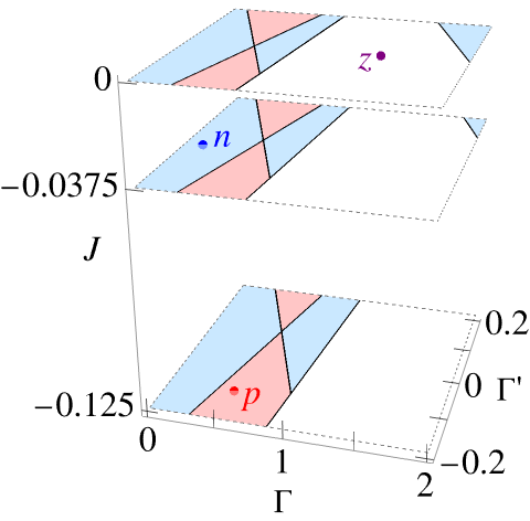
(a)

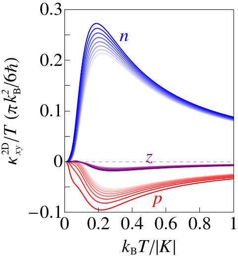
(b)

Figure 5: (a) Candidate parametrizations $p$ [73], $n$ [74], and $z$ [75] of $\alpha$-RuCl₃, with $K$ set to $-1$ and other interactions scaled accordingly, and topological phase diagrams in their neighborhoods under a magnetic field $\mathbf{h}$ along the $a$ axis ($\beta=0$). (b) Thermal Hall conductivities of $p$, $n$, and $z$ due to magnons in the polarized state under $\mathbf{h}\parallel a$, at field strengths $h$ starting from $0.18$, $0.10$, and $0.56$, respectively, and increasing to $0.32$, $0.24$, and $0.70$ in steps of $0.02$. Lighter colors indicate higher fields. $S=1/2$ is used.

Thermal Hall effect.—We discuss how the topological phase diagrams relate to experimentally measurable quantities by connecting the Chern number to the thermal Hall conductivity , which is given by [77, 78, 79]

$$\kappa_{xy}=-\frac{k_{\mathrm{B}}^{2}T}{\hbar V}\sum_{n=1}^{\mathcal{N}}\sum_{\mathbf{k}\in\mathrm{FBZ}}c_{2}\left[g\left(\frac{\hbar\omega_{n\mathbf{k}}}{k_{\mathrm{B}}T}\right)\right]\Omega_{n\mathbf{k}}$$ (5)

for magnons, where $n$ is the band index ranging from $1$ to $\mathcal{N}$ ($=2$ in our case), $c_{2}(x)=\int_{0}^{x}\mathrm{d}t\,\ln^{2}[(1+t)/t]$, $g(x)=1/(e^{x}-1)$ is the Bose-Einstein distribution, and $\Omega_{n\mathbf{k}}$ is the momentum space Berry curvature [57]. While the Chern number $\nu_{n}$ is given by the summation of $\Omega_{n\mathbf{k}}$ over $\mathbf{k}$, $\kappa_{xy}$ is given by a weighted summation of $\Omega_{n\mathbf{k}}$ with non-positive weights, as $c_{2}(x)\geq 0$ and there is a minus sign in front. One also notes that $c_{2}(x)\longrightarrow 0$ as $x\longrightarrow 0$, which implies $\kappa_{xy}\longrightarrow 0$ as $T\longrightarrow 0$, and the contribution of high energy magnons to $\kappa_{xy}$ is less important than low energy ones for $T>0$. Therefore, though $\kappa_{xy}$ is not directly proportional to $\nu$, one can very often use the latter to infer the sign of the former at low temperatures where only the lower band is thermally populated. More precisely, $\nu>0$ ($\nu<0$) means that there is an excess of positive (negative) Berry curvatures in the lower band, and by (5) the sign of $\kappa_{xy}$ is expected to be opposite to $\nu$ . On the other hand, $\nu=0$ means that the net Berry curvature is zero, so $\kappa_{xy}$ is generically small though not necessarily zero, and its sign is arbitrary.

We illustrate these ideas with three proposed parametrizations of $\alpha$-RuCl₃ in the literature, $(J,K,\Gamma,\Gamma^{\prime})=(-1,-8,4,-1)$ [73], $(-1.5,-40,5.3,-0.9)$ [74], and $(0,-6.8,9.5,0)$ [75], where energies are given in units of meV. For $\mathbf{h}\parallel a$, these parametrizations are located in the $\nu=+1$, $-1$, and $0$ regimes, respectively, so we label them by $p$, $n$, and $z$, see Fig. 5a. For each of them, we calculate $\kappa_{xy}$ as a function of $T$ at several values of $h$, see Fig. 5b. We find that $\kappa_{xy}$ is negative (positive) for $p$ ($n$) as expected, while $\kappa_{xy}$ for $z$ is one order of magnitude smaller. If we assume that the measured $\kappa_{xy}>0$ in the field induced phase under $\mathbf{h}\parallel-a$ in $\alpha$-RuCl₃ [25] is indeed determined by a dominant magnon contribution, then $p$ appears to be a more promising candidate parametrization. We also list three criteria that are conducive for a large magnon thermal Hall effect, which help us to understand the difference in $\kappa_{xy}$ for the three parametrizations, as follows. (i) The bands are topological, i.e., they carry finite Chern numbers. (ii) The excitation gap should not be too large, so that the lower band is thermally populated at low temperatures. (iii) The band gap should not be too small, so that the population of the upper band remains negligible over an extended temperature range. For instance, at the respective lowest fields, the excitation gaps of $p$, $n$, and $z$ are $0.16$, $0.19$, and $0.10$, while the band gaps are $0.07$, $0.25$, and $0.33$, in units of $\lvert K\rvert S$. $n$ and $p$ fulfill (i) and are comparable in (ii), but $n$ does better than $p$ in (iii), so $n$ yields a larger $\kappa_{xy}$. On the other hand, $z$ does better than $p$ and $n$ in (ii) and (iii), but it fails in (i), so its $\kappa_{xy}$ is small. As $h$ increases, the excitation gap becomes larger and $\kappa_{xy}$ decreases.

Discussion.—In summary, we have mapped out topological phase diagrams of Kitaev magnets polarized by in-plane magnetic fields, which reveal the Chern numbers of the magnon bands over a large parameter space. We have also discussed that topological magnons are generally expected to yield a sizable thermal Hall conductivity with sign opposite to the Chern number, when the band (excitation) gap is large (small), at low temperatures. Our results will be helpful in the search for topological magnons, as well as understanding their thermal transport signatures, in Kitaev magnets including $\alpha$-RuCl₃. While the window of a field induced KSL might be shut in many of the candidate materials, the door to topological magnons is more likely open and accessible via high fields. Although we have focused solely on magnons in this Letter, we appreciate that alternative sources of heat carriers in Kitaev magnets, such as spinons [81, 82, 83], triplons [84], phonons [85], visons [86], and some combinations [87, 88, 89, 90, 91], have been proposed in the literature. One particularly interesting future direction is to investigate the interplay between different types of topological excitations, whether they cooperate (cancel) with each other and lead to a large (small) thermal Hall effect [92].

Supplemental Material: Topological phase diagrams of in-plane field polarized Kitaev magnets

Li Ern Chern¹ and Claudio Castelnovo¹

¹T.C.M. Group, Cavendish Laboratory, University of Cambridge, Cambridge CB3 0HE, United Kingdom

S1 Linear Spin Wave Theory

In the linear spin wave analysis, one first rotates the local coordinate frame defined at each magnetic site such that the $z$-axis align with the spin [60], while the $x$ and $y$ axes can be chosen freely as long as they are orthogonal and $\hat{\mathbf{z}}=\hat{\mathbf{x}}\times\hat{\mathbf{y}}$ [70]. For the polarized state with field angle $\beta$, the axes of the rotated coordinates are defined by $\hat{\mathbf{z}}=\hat{\mathbf{a}}\cos\beta+\hat{\mathbf{b}}\sin\beta$, $\hat{\mathbf{x}}=-\hat{\mathbf{c}}$, $\hat{\mathbf{y}}=-\hat{\mathbf{a}}\sin\beta+\hat{\mathbf{b}}\cos\beta$, where $\hat{\mathbf{a}}$, $\hat{\mathbf{b}}$, and $\hat{\mathbf{c}}$ are unit vectors along the crystallographic axes $a$, $b$, and $c$, respectively, see Fig. 2a. One then performs Holstein-Primakoff transformation [59] to represent the spins in terms of bosons (i.e., magnons), perform a $1/S$ expansion of the Hamiltonian ($\sim S^{2}$ in the classical limit), and discard terms are of orders lower than $S$. These procedures are well established and described in details elsewhere (see Refs. [78, 62, 40] for example), so we do not repeat them here.

For the $JK\Gamma\Gamma^{\prime}$ model (1) under an in-plane magnetic field $(h_{a},h_{b},h_{c})=h(\cos\beta,\sin\beta,0)$, the linear spin wave Hamiltonian of the polarized state is given by $H=(S/2)\sum_{\mathbf{k}}\Psi_{\mathbf{k}}^{\dagger}\mathcal{H}_{\mathbf{k}}\Psi_{\mathbf{k}}$, where $\Psi_{\mathbf{k}}=(b_{1\mathbf{k}},b_{2\mathbf{k}},b_{1-\mathbf{k}}^{\dagger},b_{2-\mathbf{k}}^{\dagger})$ and $\mathcal{H}_{\mathbf{k}}$ is a four dimensional Hermitian matrix,

$$\mathcal{H}_{\mathbf{k}}=\begin{pmatrix}\mathcal{A}_{\mathbf{k}}&\mathcal{B}_{\mathbf{k}}\\ \mathcal{B}_{-\mathbf{k}}^{*}&\mathcal{A}_{-\mathbf{k}}^{\mathrm{T}}\end{pmatrix},$$ (S1a)

$$\mathcal{A}_{\mathbf{k}}=\frac{1}{2}\begin{pmatrix}2(h-c_{1})&c_{2}f_{\mathbf{k}}^{*}+c_{3}+c_{4}g_{\mathbf{k}}^{*}\\ c_{2}f_{\mathbf{k}}+c_{3}+c_{4}g_{\mathbf{k}}&2(h-c_{1})\end{pmatrix},$$ (S1b)

$$\mathcal{B}_{\mathbf{k}}=\frac{1}{2}\begin{pmatrix}0&c_{5}f_{\mathbf{k}}^{*}-c_{3}-c_{4}g_{\mathbf{k}}^{*}+2i\big{[}c_{6}(f_{\mathbf{k}}^{*}-3)+c_{7}g_{\mathbf{k}}^{*}\big{]}\\ c_{5}f_{\mathbf{k}}-c_{3}-c_{4}g_{\mathbf{k}}+2i\big{[}c_{6}(f_{\mathbf{k}}-3)+c_{7}g_{\mathbf{k}}\big{]}&0\end{pmatrix},$$ (S1c)

where $c_{i}$ are (real) linear combinations of the couplings, while $f_{\mathbf{k}}$ and $g_{\mathbf{k}}$ are functions of the (crystal) momentum, see (LABEL:cidefine) and related discussions in the main text. To obtain the linear spin wave dispersion, $\mathcal{H}_{\mathbf{k}}$ has to be diagonalized by a Bogoliubov transformation $T_{\mathbf{k}}$ satisfying $T_{\mathbf{k}}\eta T_{\mathbf{k}}^{\dagger}=\eta$, where $\eta=\mathrm{diag}(1,1,-1,-1)$, in order to preserve the commutation relation of bosons. The magnon bands are given by

$$\omega_{\pm}(\mathbf{k})=\frac{S}{2}\sqrt{E(\mathbf{k})\pm\Delta(\mathbf{k})},$$ (S2)

where $E(\mathbf{k})$ and $\Delta(\mathbf{k})$ are defined in (2a) and (LABEL:Dksquaredefine) in the main text.

We consider a stable polarized state, where the excitation gap $\min_{\mathbf{k}}\omega_{-}(\mathbf{k})$ is greater than zero. As the field strength $h$ increases, the excitation gap should increase as well, so that the polarized state becomes more stable, rather than undergoing a magnon instability in which the excitation gap vanishes. Based on this physical expectation, we can assume

$$h-c_{1}>0$$ (S3)

always, which is argued as follows. Eq. (S3) obviously holds for $c_{1}\leq 0$ for all $h$. For $c_{1}>0$, assuming that a finite excitation gap is possible for some $h<c_{1}$, we can then dial up $h$ such that $h=c_{1}$. At the $\mathrm{K}$ or $\mathrm{K}^{\prime}$ point, where $f_{\mathbf{k}}=0$, we will have $\omega_{\pm}(\mathbf{k})=\sqrt{-4\lvert-3c_{6}+c_{7}g_{\mathbf{k}}\rvert^{2}}$, which is either zero or imaginary, neither being physically sensible. Therefore, magnon stability is only consistent with $h-c_{1}>0$.

A quick inspection of (LABEL:Dksquaredefine) reveals that $\Delta^{2}(\mathbf{k})$ consists of a field dependent part and a field independent part. With the assumption (S3), we now claim that if $\Delta(\mathbf{k})=0$, then it is only physically sensible that $c_{2}f_{\mathbf{k}}+c_{3}+c_{4}g_{\mathbf{k}}=0$, unless the system sits at a critical point where a transition to the polarized state occurs. Suppose that the contrary is true, i.e., $\Delta(\mathbf{k})=0$ and $c_{2}f_{\mathbf{k}}+c_{3}+c_{4}g_{\mathbf{k}}\neq 0$ at some $h=h_{*}$, with $h_{*}-c_{1}>0$. The field dependent part, which is positive, must cancel the field independent part exactly in $\Delta^{2}(\mathbf{k})$. Let $h^{\prime}=h_{*}-\epsilon$ with $0<\epsilon<h_{*}-c_{1}$. We have $h^{\prime}-c_{1}>0$, but $\Delta^{2}(\mathbf{k})<0$ at $h=h^{\prime}$, i.e., $\omega_{\pm}(\mathbf{k})$ develops an imaginary component, which is unphysical. Therefore, $h$ cannot be less than $h_{*}$. In case $h_{*}$ marks the phase boundary, we can further increase the field to some $h>h_{*}$ to obtain a stable polarized state. We have thus established

Proposition 1. Under the stability requirement $h-c_{1}>0$, $c_{2}f_{\mathbf{k}}+c_{3}+c_{4}g_{\mathbf{k}}=0$ is a necessary condition for $\Delta(\mathbf{k})=0$.

We refer to the gap between the upper and lower magnon bands, $\min_{\mathbf{k}}[\omega_{+}(\mathbf{k})-\omega_{-}(\mathbf{k})]\geq 0$, as the band gap, which is not to be confused with the excitation gap. From (S2), we see that the band gap vanishes if and only if $\Delta(\mathbf{k})=0$ for some $\mathbf{k}=\mathbf{k}_{*}$. For a fixed set of couplings $\{J,K,\Gamma,\Gamma^{\prime}\}$, the analysis in the previous two paragraphs implies, within a stable polarized state,

Corollary 1. If the band gap is zero, then it remains zero as $h$ varies;

Corollary 2. If the band gap is finite, then it remains finite as $h$ varies, unless $h\longrightarrow\infty$ while the couplings stay finite.

To see why these observations are useful, we first note that the Chern number is a topological invariant that can never change as long as a finite band gap is maintained. A topological phase transition can only occur when the band gap vanishes. Therefore, within a stable in-plane field polarized state and for a finite $h$, Corollaries 1 and 2 respectively imply

Lemma 1. If a topological transition exists, the phase boundary, which must be a parameter region where the band gap goes to zero, is independent of the field strength;

Lemma 2. The Chern number of each magnon band, which is well defined when the band gap is finite, is independent of the field strength.

We are now ready to solve analytically for regions in the $JK\Gamma\Gamma^{\prime}$ parameter space where the band gap vanishes, which are potential phase boundaries for topological transitions.

$\beta=0$. With $c_{4}=0$ and $c_{6}=0$, (LABEL:Dksquaredefine) reads

$$\Delta^{2}(\mathbf{k})=16(h-c_{1})^{2}\big{\lvert}c_{2}f_{\mathbf{k}}+c_{3}\big{\rvert}^{2}+(c_{2}+c_{5})\big{[}(c_{2}+c_{5})c_{3}^{2}(f_{\mathbf{k}}^{*}-f_{\mathbf{k}})^{2}+8c_{3}c_{7}^{2}(g_{\mathbf{k}}f_{\mathbf{k}}^{*}-g_{\mathbf{k}}^{*}f_{\mathbf{k}})(g_{\mathbf{k}}-g_{\mathbf{k}}^{*})+4(c_{2}-c_{5})c_{7}^{2}(g_{\mathbf{k}}f_{\mathbf{k}}^{*}-g_{\mathbf{k}}^{*}f_{\mathbf{k}})^{2}\big{]}.$$ (S4)

The band gap is zero if and only if there is at least one $\mathbf{k}$ such that $\Delta(\mathbf{k})=0$. According to Proposition 1, we require

$$c_{2}f_{\mathbf{k}}+c_{3}=0,$$ (S5)

which makes the field dependent part of $\Delta^{2}(\mathbf{k})$ zero. The field independent part should be zero as well. We solve these conditions on a case by case basis.

Case 1. $c_{2}=0$. We must have $c_{3}=0$. When $\mathbf{k}=\mathrm{K},\mathrm{K}^{\prime}$, $f_{\mathbf{k}}=0$, and $\Delta^{2}(\mathbf{k})=0$ is satisfied.

Case 2. $c_{2}\neq 0$.

Case 2.1. $c_{3}=0$. When $\mathbf{k}=\mathrm{K},\mathrm{K}^{\prime}$, $f_{\mathbf{k}}=0$, and $\Delta^{2}(\mathbf{k})=0$ is satisfied.

Case 2.2. $c_{3}\neq 0$. The real and imaginary parts of (S5) respectively read

$$c_{2}(1+\cos k_{1}+\cos k_{2})+c_{3} =0,$$ (S6a)

$$c_{2}(\sin k_{1}+\sin k_{2}) =0.$$ (S6b)

(S6b) implies $k_{2}=-k_{1}+2\pi$ or $k_{2}=k_{1}+\pi$.

Case 2.2.1. $k_{2}=-k_{1}+2\pi$. Eq. (S6a) becomes $c_{2}(1+2\cos k_{1})+c_{3}=0$, which only admits a solution when $-1\leq-c_{3}/c_{2}\leq 3$. In this case, $f_{\mathbf{k}}=-c_{3}/c_{2}$, and (S4) becomes

$$\Delta^{2}(\mathbf{k})=\left(\frac{8c_{3}}{c_{2}}\right)^{2}c_{7}^{2}(c_{2}+c_{5})^{2}\sin^{2}k_{1}.$$ (S7)

The first bracket on the right hand side is assumed to be nonzero, so $\Delta^{2}(\mathbf{k})=0$ if and only if (i) $c_{7}=0$, (ii) $c_{2}+c_{5}=0$, or (iii) $\sin k_{1}=0$, which implies $k_{1}=0,\pi$, which in turn implies $3c_{2}+c_{3}=0$ or $-c_{2}+c_{3}=0$, respectively.

Case 2.2.2. $k_{2}=k_{1}+\pi$. Eq. (S6a) reads $c_{2}+c_{3}=0$. In this case, $f_{\mathbf{k}}=1$ and $g_{\mathbf{k}}$ is real at $k_{1}=0,\pi$, which yield $\Delta^{2}(\mathbf{k})=0$ by (S4).

Collecting all the results, the parameter regions where the band gap vanishes satisfy one of the following equations: (I) $c_{3}=0$, (II) $3c_{2}+c_{3}=0$, (III) $-c_{2}+c_{3}=0$, (IV,V) $c_{2}+c_{3}=0$, (VI) $c_{2}+c_{5}=0$ if $-1\leq-c_{3}/c_{2}\leq 3$, and (VII) $c_{7}=0$ if $-1\leq-c_{3}/c_{2}\leq 3$. The reason that we use two labels IV and V for the equation $c_{2}+c_{3}=0$ will be clear when we discuss the case $0<\beta\leq\pi/6$.

$0<\beta\leq\pi/6$. The band gap is zero if and only if there is at least one $\mathbf{k}$ such that $\Delta(\mathbf{k})=0$ [see (LABEL:Dksquaredefine) in the main text]. According to Proposition 1, we require

$$c_{2}f_{\mathbf{k}}+c_{3}+c_{4}g_{\mathbf{k}}=0,$$ (S8)

which makes the field dependent part of $\Delta^{2}(\mathbf{k})$ zero. The field independent part should be zero as well. We solve these conditions on a case by case basis.

Case 1. $K+2\Gamma-2\Gamma^{\prime}=0$. Then, $c_{3}=0$ and $c_{4}=0$. At $\mathbf{k}=\mathrm{K},\mathrm{K}^{\prime}$, $f_{\mathbf{k}}=0$, and $\Delta^{2}(\mathbf{k})=0$ from (LABEL:Dksquaredefine).

Case 2. $K+2\Gamma-2\Gamma^{\prime}\neq 0$. Then, $c_{3}\neq 0$ and $c_{4}\neq 0$. The real and imaginary parts of (S8) respectively read

$$(c_{2}+c_{3})+(c_{2}+c_{4})\cos k_{1}+(c_{2}-c_{4})\cos k_{2} =0,$$ (S9a)

$$(c_{2}+c_{4})\sin k_{1}+(c_{2}-c_{4})\sin k_{2} =0.$$ (S9b)

Case 2.1. $c_{2}=c_{4}$. Eq. (S9b) implies $k_{1}=0,\pi$. Substituting $k_{1}=\pi$ in (S9a) leads to $c_{3}-c_{4}=0$, or $K+2\Gamma-2\Gamma^{\prime}=0$, a contradiction. We thus discard $k_{1}=\pi$. Substituting $k_{1}=0$ in (S9a) leads to $c_{3}+3c_{4}=0$, which holds only at $\beta=\pi/12$. We can then choose $k_{2}=0,\pi$ so that $f_{\mathbf{k}}$ and $g_{\mathbf{k}}$ are real, and $\Delta^{2}(\mathbf{k})=0$ is satisfied.

Case 2.2. $c_{2}=-c_{4}$. Eq. (S9b) implies $k_{2}=0,\pi$. Substituting $k_{2}=0$ in (S9a) leads to $c_{3}-3c_{4}=0$, or $K+2\Gamma-2\Gamma^{\prime}=0$, a contradiction. We thus discard $k_{2}=0$. Substituting $k_{2}=\pi$ in (S9a) leads to $c_{3}+c_{4}=0$, which holds only at $\beta=\pi/6$. We can then choose $k_{1}=0,\pi$ so that $f_{\mathbf{k}}$ and $g_{\mathbf{k}}$ are real, and $\Delta^{2}(\mathbf{k})=0$ is satisfied.

Case 2.3. $\lvert c_{2}\rvert\neq\lvert c_{4}\rvert$.

Case 2.3.1. $(k_{1},k_{2})\in\{(0,0),(0,\pi),(\pi,0),(\pi,\pi)\}$. Eq. (S9b) is satisfied. Eq. (S9a) implies $3c_{2}+c_{3}=0$, $c_{2}+c_{3}+2c_{4}=0$, $c_{2}+c_{3}-2c_{4}=0$, or $-c_{2}+c_{3}=0$, respectively. Since $f_{\mathbf{k}}$ and $g_{\mathbf{k}}$ are real, $\Delta^{2}(\mathbf{k})=0$ is satisfied.

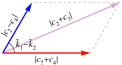
Figure S1: Eq. (S11) can be interpreted as the sum of two vectors.

Case 2.3.2. $(k_{1},k_{2})\notin\{(0,0),(0,\pi),(\pi,0),(\pi,\pi)\}$. We write (S9a) and (S9b) as

$$\lvert c_{2}+c_{4}\rvert\cos\tilde{k}_{1}+\lvert c_{2}-c_{4}\rvert\cos\tilde{k}_{2} =-(c_{2}+c_{3}),$$ (S10a)

$$\lvert c_{2}+c_{4}\rvert\sin\tilde{k}_{1}+\lvert c_{2}-c_{4}\rvert\sin\tilde{k}_{2} =0,$$ (S10b)

where $\tilde{k}_{1}=k_{1}$ if $c_{2}+c_{4}>0$ and $\tilde{k}_{1}=k_{1}+\pi$ if $c_{2}+c_{4}<0$; $\tilde{k}_{2}$ is defined in a similar way. Squaring both sides of (S10a) and (S10b), and adding up the results lead to

$$\lvert c_{2}+c_{4}\rvert^{2}+\lvert c_{2}-c_{4}\rvert^{2}+2\lvert c_{2}+c_{4}\rvert\lvert c_{2}-c_{4}\rvert\cos(\tilde{k}_{1}-\tilde{k}_{2})=\lvert c_{2}+c_{3}\rvert^{2}.$$ (S11)

(S11) can be interpreted as a summation of two vectors, one of length $\lvert c_{2}+c_{4}\rvert$ and the other $\lvert c_{2}-c_{4}\rvert$, with an angle $\tilde{k}_{1}-\tilde{k}_{2}$ in between, which results in a vector of length $\lvert c_{2}+c_{3}\rvert$, see Fig. S1. With this interpretation, we deduce that (S11) admits a solution when

$$\big{\lvert}\lvert c_{2}+c_{4}\rvert-\lvert c_{2}-c_{4}\rvert\big{\rvert}\leq\lvert c_{2}+c_{3}\rvert\leq\lvert c_{2}+c_{4}\rvert+\lvert c_{2}-c_{4}\lvert.$$ (S12)

The right (left) equality holds when the two vectors (anti-)align, i.e., $\tilde{k}_{1}-\tilde{k}_{2}=0$ ($\pi$), where the resulting vector reaches its longest (shortest) possible length. The equalities in (S12), however, require $(k_{1},k_{2})\in\{(0,0),(0,\pi),(\pi,0),(\pi,\pi)\}$, which can be seen from (S10a). This is a contradiction, but we note that these momenta have been covered in Case 2.3.1. We can thus focus on the inequalities in (S12), and assume that they are satisfied. From (S11),

$$\cos(\tilde{k}_{1}-\tilde{k}_{2}) =\frac{\lvert c_{2}+c_{3}\rvert^{2}-\lvert c_{2}+c_{4}\rvert^{2}-\lvert c_{2}-c_{4}\rvert^{2}}{2\lvert c_{2}+c_{4}\rvert\lvert c_{2}-c_{4}\rvert},$$ (S13a)

$$\sin(\tilde{k}_{1}-\tilde{k}_{2}) =\pm\sqrt{1-\cos^{2}(\tilde{k}_{1}-\tilde{k}_{2})}.$$ (S13b)

Substituting (S10b) in (S10a) yields

$$\sin\tilde{k}_{1} =-\frac{\lvert c_{2}-c_{4}\rvert}{c_{2}+c_{3}}\sin(\tilde{k}_{1}-\tilde{k}_{2}),$$ (S14a)

$$\sin\tilde{k}_{2} =\frac{\lvert c_{2}+c_{4}\rvert}{c_{2}+c_{3}}\sin(\tilde{k}_{1}-\tilde{k}_{2}).$$ (S14b)

Notice that $c_{2}+c_{3}\neq 0$ due to (4). From (S14a) and (S14b),

$$-\sin(\tilde{k}_{1}-\tilde{k}_{2})\cos\tilde{k}_{1}+\cos(\tilde{k}_{1}-\tilde{k}_{2})\sin\tilde{k}_{1}=\frac{\lvert c_{2}+c_{4}\rvert}{c_{2}+c_{3}}\sin(\tilde{k}_{1}-\tilde{k}_{2})\iff\cos\tilde{k}_{1}=-\frac{\lvert c_{2}+c_{4}\rvert}{c_{2}+c_{3}}-\frac{\lvert c_{2}-c_{4}\rvert}{c_{2}+c_{3}}\cos(\tilde{k}_{1}-\tilde{k}_{2}),$$ (S15a)

$$\sin(\tilde{k}_{1}-\tilde{k}_{2})\cos\tilde{k}_{2}+\cos(\tilde{k}_{1}-\tilde{k}_{2})\sin\tilde{k}_{2}=-\frac{\lvert c_{2}-c_{4}\rvert}{c_{2}+c_{3}}\sin(\tilde{k}_{1}-\tilde{k}_{2})\iff\cos\tilde{k}_{2}=-\frac{\lvert c_{2}-c_{4}\rvert}{c_{2}+c_{3}}-\frac{\lvert c_{2}+c_{4}\rvert}{c_{2}+c_{3}}\cos(\tilde{k}_{1}-\tilde{k}_{2}).$$ (S15b)

In order for (S14a), (S14b), (S15a), and (S15b) to admit a solution $(\tilde{k}_{1},\tilde{k}_{2})$, we need to verify that the absolute values of the right hand sides are less than or equal to unity. We calculate

$$\sin^{2}\tilde{k}_{1}+\cos^{2}\tilde{k}_{1}=\frac{\lvert c_{2}-c_{4}\rvert^{2}+\lvert c_{2}+c_{4}\rvert^{2}+2\lvert c_{2}+c_{4}\rvert\lvert c_{2}-c_{4}\rvert\cos(\tilde{k}_{1}-\tilde{k}_{2})}{\lvert c_{2}+c_{3}\rvert^{2}}=1,$$ (S16a)

$$\sin^{2}\tilde{k}_{2}+\cos^{2}\tilde{k}_{2}=\frac{\lvert c_{2}+c_{4}\rvert^{2}+\lvert c_{2}-c_{4}\rvert^{2}+2\lvert c_{2}-c_{4}\rvert\lvert c_{2}+c_{4}\rvert\cos(\tilde{k}_{1}-\tilde{k}_{2})}{\lvert c_{2}+c_{3}\rvert^{2}}=1,$$ (S16b)

where the last equalities follow from (S11). If the squares of two real numbers add up to unity, then each must be less than or equal to unity. We have demonstrated that there indeed exists $(\tilde{k}_{1},\tilde{k}_{2})$, defined implicitly via (S14a), (S14b), (S15a), and (S15b) in conjunction with (S13a) and (S13b), which solves (S10a) and (S10b).

Substituting (S8) in (LABEL:Dksquaredefine),

$$\Delta^{2}(\mathbf{k})=-\frac{4(c_{2}+c_{5})^{2}(c_{3}c_{7}+3c_{4}c_{6})^{2}(f_{\mathbf{k}}-f_{\mathbf{k}}^{*})^{2}}{c_{4}^{2}}=-\frac{\cos^{2}(3\beta)(c_{2}+c_{5})^{2}(K-\Gamma+\Gamma^{\prime})^{2}(K+2\Gamma-2\Gamma^{\prime})^{2}(f_{\mathbf{k}}-f_{\mathbf{k}}^{*})^{2}}{6c_{4}^{2}}.$$ (S17)

If $\beta=\pi/6$, then $\cos(3\beta)=0$, and $\Delta^{2}(\mathbf{k})=0$ is satisfied. For $0<\beta<\pi/6$, $\cos(3\beta)\neq 0$. $f_{\mathbf{k}}-f_{\mathbf{k}}^{*}$ vanishes if and only if $f_{\mathbf{k}}$ is real, but this implies, via (S9b), $c_{4}=0$ or $(k_{1},k_{2})\in\{(0,0),(0,\pi),(\pi,0),(\pi,\pi)\}$, both of which violate the initial assumptions. Thus $f_{\mathbf{k}}-f_{\mathbf{k}}^{*}\neq 0$. Furthermore, $K+2\Gamma-2\Gamma^{\prime}\neq 0$ by assumption. Therefore, $\Delta^{2}(\mathbf{k})=0$ if and only if (i) $c_{2}+c_{5}=0$ or (ii) $K-\Gamma+\Gamma^{\prime}=0$.

Collecting all the results, for $0<\beta<\pi/6$, the parameter regions where the band gap vanishes satisfy one of the following equations: (I) $K+2\Gamma-2\Gamma^{\prime}=0$, (II) $3c_{2}+c_{3}=0$, (III) $-c_{2}+c_{3}=0$, (IV) $c_{2}+c_{3}+2c_{4}=0$, (V) $c_{2}+c_{3}-2c_{4}=0$, (VI) $c_{2}+c_{5}=0$ if (S12) holds, and (VII) $K-\Gamma+\Gamma^{\prime}=0$ if (S12) holds. Setting $\beta=0$, these criteria are equivalent to those solved earlier for $\beta=0$, which was the reason that we used two labels IV and V for $c_{2}+c_{3}=0$, as $c_{4}=0$ there. On the other hand, for $\beta=\pi/6$, the gap is zero whenever (I) or (S12) holds. (I-VII) are expressed in terms of the couplings and the field angle in Table 1.

S2 Computation of Chern number

The Berry curvature of the $n^{\mathrm{th}}$ magnon band at the momentum $\mathbf{k}$ is defined in terms of the Bogoliubov transformation $T_{\mathbf{k}}$ as [78]

$$\Omega_{n\mathbf{k}}=i\epsilon_{\mu\nu}\left(\eta\frac{\partial T_{\mathbf{k}}^{\dagger}}{\partial k_{\mu}}\eta\frac{\partial T_{\mathbf{k}}}{\partial k_{\nu}}\right)_{nn},$$ (S18)

where $\epsilon$ is the totally antisymmetric tensor and $\mu,\nu\in\{x,y\}$. (Caution: The expression within the brackets on the right hand side is a matrix, and the subscript $nn$ means the entry at the $n^{\mathrm{th}}$ row and the $n^{\mathrm{th}}$ column; $n$ is not a dummy index that is being summed over.) Integrating (S18) over the magnetic Brillouin zone gives the Chern number of the $n^{\mathrm{th}}$ band,

$$\nu_{n}=\frac{1}{2\pi}\int_{\mathrm{MBZ}}\mathrm{d}k_{x}\mathrm{d}k_{y}\,\Omega_{n\mathbf{k}}.$$ (S19)

This section explains the method that we use to compute the Chern number in a discretized Brillouin zone, which was introduced in Ref. [65] and based on a $U(1)$ lattice gauge theory (see also Refs. [53, 66]). The Berry curvature (S18) multiplied by the integral measure, $\Omega_{n\mathbf{k}}\,\mathrm{d}k_{x}\mathrm{d}k_{y}$, is invariant under a coordinate transformation [64], e.g.

$$\Omega_{n}(k_{x},k_{y})\,\mathrm{d}k_{x}\mathrm{d}k_{y}=F_{n}(k_{1},k_{2})\,\mathrm{d}k_{1}\mathrm{d}k_{2},$$ (S20a)

$$F_{n}(k_{1},k_{2})\equiv i\left(\eta\frac{\partial T_{\mathbf{k}}^{\dagger}}{\partial k_{1}}\eta\frac{\partial T_{\mathbf{k}}}{\partial k_{2}}-\eta\frac{\partial T_{\mathbf{k}}^{\dagger}}{\partial k_{2}}\eta\frac{\partial T_{\mathbf{k}}}{\partial k_{1}}\right)_{nn}.$$ (S20b)

(More formally, the differential 2-form $\Omega_{n\mathbf{k}}\,\mathrm{d}k_{x}\wedge\mathrm{d}k_{y}$ is coordinate independent.) Let $\mathcal{N}$ be the number of sites per magnetic unit cell, in particular $\mathcal{N}=2$ for the polarized state. If there is a finite magnon pairing term, then the $2\mathcal{N}$ dimensional Hamiltonian matrix $\mathcal{H}_{\mathbf{k}}$ has a particle-hole redundancy by construction. The columns of the $2\mathcal{N}$ dimensional Bogoliubov transformation matrix $T_{\mathbf{k}}$ are arranged such that the first (last) $\mathcal{N}$ columns belong to the particle (hole) sector.

Let $\lvert n(\mathbf{k})\rangle\equiv(\mathbf{u}_{n}(\mathbf{k}),\mathbf{v}_{n}(\mathbf{k}))$ be the $n^{\mathrm{th}}$ vector of $T_{\mathbf{k}}$. We have introduced the $\mathcal{N}$ dimensional vector $\mathbf{u}_{n}(\mathbf{k})$ [$\mathbf{v}_{n}(\mathbf{k})$] as the first [second] half of $\lvert n(\mathbf{k})\rangle$. In the rest of this section, we focus on the particle sector, i.e., $1\leq n\leq\mathcal{N}$. Next, we define the Berry connection of the $n^{\mathrm{th}}$ band at the momentum $\mathbf{k}$ as

$$A_{n,\lambda}(\mathbf{k})=i\langle n(\mathbf{k})\rvert\eta\partial_{k_{\lambda}}\lvert n(\mathbf{k})\rangle=i\left[\mathbf{u}_{n}^{\dagger}(\mathbf{k})\partial_{k_{\lambda}}\mathbf{u}_{n}(\mathbf{k})-\mathbf{v}_{n}^{\dagger}(\mathbf{k})\partial_{k_{\lambda}}\mathbf{v}_{n}(\mathbf{k})\right],$$ (S21)

where $\lambda=1,2$. Since $\langle n(\mathbf{k})\rvert\eta\lvert n(\mathbf{k})\rangle=1$, $\langle n(\mathbf{k})\rvert\eta\partial_{k_{\lambda}}\lvert n(\mathbf{k})\rangle$ is purely imaginary and hence $A_{n,\lambda}$ is purely real. Using the definition (S20b), it can be straightforwardly verified that

$$F_{n}(\mathbf{k})=\left[\partial_{k_{1}}A_{n,2}(\mathbf{k})-\partial_{k_{2}}A_{n,1}(\mathbf{k})\right].$$ (S22)

On the discretized Brillouin zone, suppose that the spacings of momenta along the $k_{1}$ and $k_{2}$ directions are $\delta k_{1}$ and $\delta k_{2}$, respectively. If we make $\delta k_{\lambda}$ small enough, we can approximate (S21) and (S22) as

$$A_{n,\lambda}\,\delta k_{\lambda} \approx i\left[\langle n(\mathbf{k})\lvert\eta\rvert n(\mathbf{k}+\delta k_{\lambda}\hat{\mathbf{\lambda}})\rangle-1\right],$$ (S23a)

$$F_{n}(\mathbf{k})\,\delta k_{1}\delta k_{2} \approx\left[A_{n,2}(\mathbf{k}+\delta k_{1}\hat{1})-A_{n,2}(\mathbf{k})\right]\delta k_{2}-\left[A_{n,1}(\mathbf{k}+\delta k_{2}\hat{2})-A_{n,1}(\mathbf{k})\right]\delta k_{1}.$$ (S23b)

We define the $U(1)$ link variable

$$U_{\lambda}(\mathbf{k})=\frac{\langle n(\mathbf{k})\rvert\eta\lvert n(\mathbf{k}+\delta k_{\lambda}\hat{\lambda})\rangle}{\left\lvert\langle n(\mathbf{k})\rvert\eta\lvert n(\mathbf{k}+\delta k_{\lambda}\hat{\lambda})\rangle\right\rvert}=\frac{\langle n(\mathbf{k})\rvert\eta\lvert n(\mathbf{k}+\delta k_{\lambda}\hat{\lambda})\rangle}{1+O(\delta k_{\lambda}^{2})}\approx\exp\left[-iA_{n,\lambda}(\mathbf{k})\delta k_{\lambda}\right],$$ (S24)

where, to obtain the second equality, we have expanded $\langle n(\mathbf{k})\rvert\eta\lvert n(\mathbf{k}+\delta k_{\lambda}\hat{\lambda})\rangle\approx 1+\langle n(\mathbf{k})\rvert\eta\partial_{k_{\lambda}}\lvert n(\mathbf{k})\rangle\delta k_{\lambda}$ and used the fact that $\langle n(\mathbf{k})\rvert\eta\partial_{k_{\lambda}}\lvert n(\mathbf{k})\rangle$ is imaginary. Eq. (S23b) can be expressed in terms of (S24) as

$$F_{n}(\mathbf{k})\delta k_{1}\delta k_{2}\approx i\ln\left[U_{1}(\mathbf{k})U_{2}(\mathbf{k}+\delta k_{1}\hat{1})U_{1}^{-1}(\mathbf{k}+\delta k_{2}\hat{2})U_{2}^{-1}(\mathbf{k})\right].$$ (S25)

Finally, the Chern number of the $n^{\mathrm{th}}$ magnon band (S19) is calculated as

$$\nu_{n}\approx\frac{1}{2\pi}\sum_{\mathbf{k}\in\mathrm{MBZ}}F_{n}(\mathbf{k})\,\delta k_{1}\delta k_{2}.$$ (S26)

The main advantage of using (S25) over (S20b) for computing Chern numbers is that the former is manifestly gauge invariant, i.e., it is unaffected by $\lvert n(\mathbf{k})\rangle\longrightarrow\exp[-i\chi(\mathbf{k})]\lvert n(\mathbf{k})\rangle$ as desired, while the latter requires explicit gauge fixings when taking the differences of $T_{\mathbf{k}}$ to approximate the derivatives.

We mention in passing that the thermal Hall conductivity (5) can also be calculated within this framework,

$$\kappa_{xy}^{\mathrm{2D}}\approx-\frac{k_{\mathrm{B}}^{2}T}{(2\pi)^{2}\hbar}\sum_{n=1}^{\mathcal{N}}\sum_{\mathbf{k}\in\mathrm{MBZ}}c_{2}\left[g\left(\frac{\hbar\omega_{n\mathbf{k}}}{k_{\mathrm{B}}T}\right)\right]F_{n}(\mathbf{k})\,\delta k_{1}\delta k_{2},$$ (S27)

with $F_{n}(\mathbf{k})$ given in (S25).

S3 Symmetries

In this section, we discuss how topological phase diagrams for different in-plane field directions are related by symmetries of the $JK\Gamma\Gamma^{\prime}$ model, which, in the absence of an external magnetic field, includes a time reversal $\mathcal{T}$ symmetry, a $C_{3}$ symmetry about the $c$ axis, and a $C_{2}$ symmetry about the $b$ axis. Let $\mathbf{J}=(J,K,\Gamma,\Gamma^{\prime})$. The Hamiltonian matrix (S1a) is a function of the parameter $\mathbf{J}$, the field $\mathbf{h}$, and the momentum $\mathbf{k}$, so we write it as $\mathcal{H}_{\mathbf{k}}(\mathbf{J},h,\beta)$.

Consider a $C_{2}$ rotation of the field, i.e., $\beta=\pi/2-\tilde{\beta}\longrightarrow\pi/2+\tilde{\beta}$, at a fixed parameter $\mathbf{J}$. Under $C_{2}$, we also have the mapping $k_{1}\longleftrightarrow k_{2}$, or equivalently $k_{x}\longrightarrow-k_{x}$ and $k_{y}\longrightarrow k_{y}$. By this observation or by explicit calculation [40], one can show that $\mathcal{H}_{(k_{x},k_{y})}(\mathbf{J},h,\pi/2+\tilde{\beta})=\mathcal{H}_{(-k_{x},k_{y})}(\mathbf{J},h,\pi/2-\tilde{\beta})$. As a consequence, if the band gap is zero (finite) at $(\mathbf{J},h,\pi/2+\tilde{\beta})$, then it is also zero (finite) at $(\mathbf{J},h,\pi/2-\tilde{\beta})$. Assume that the band gap is finite. The Bogoliubov transformations are related by $T_{(k_{x},k_{y})}(\mathbf{J},h,\pi/2+\tilde{\beta})=T_{(-k_{x},k_{y})}(\mathbf{J},h,\pi/2-\tilde{\beta})$. By (S18) and (S19), we have $\Omega_{n(k_{x},k_{y})}(\mathbf{J},h,\pi/2+\tilde{\beta})=-\Omega_{n(-k_{x},k_{y})}(\mathbf{J},h,\pi/2-\tilde{\beta})$ and $\nu_{n}(\mathbf{J},\pi/2+\tilde{\beta})=-\nu_{n}(\mathbf{J},\pi/2-\tilde{\beta})$ for the Berry curvatures and the Chern numbers. In other words, the Chern number of the $n^{\mathrm{th}}$ magnon band in the polarized state switches sign when the field direction is changed to its $C_{2}$ counterpart. Theorems 1 and 2 in Ref. [40] follow from this.

Consider a $C_{3}$ rotation of the field, i.e., $\beta\longrightarrow\beta+2\pi/3$, at a fixed parameter $\mathbf{J}$. This amounts to holding the field fixed in space while cyclically permuting the $x$, $y$, and $z$ spin components. Therefore, $C_{3}$ preserves the band gap (which can be either zero or finite) and the Chern number.

Consider the action of time reversal $\mathcal{T}$, i.e., $\mathbf{h}\longrightarrow-\mathbf{h}$ or, specifically for in-plane fields, $\beta\longrightarrow\beta+\pi$, at a fixed parameter $\mathbf{J}$. We have $\mathcal{H}_{\mathbf{k}}(\mathbf{J},h,\beta+\pi)=\mathcal{H}_{-\mathbf{k}}^{*}(\mathbf{J},h,\beta)$ by a theorem proved in Ref. [41]. Therefore, $\mathcal{T}$ preserves the band gap (which can be either zero or finite) but flips the sign of the Chern number.

Finally, consider flipping the signs of all couplings, i.e., $\mathbf{J}\longrightarrow-\mathbf{J}$, at a fixed field direction $\beta$. Following Ref. [52], we introduce

$$U=\begin{pmatrix}0&1&0&0\\ -1&0&0&0\\ 0&0&0&1\\ 0&0&-1&0\end{pmatrix}=\mathbf{1}\otimes(i\sigma_{2}),$$ (S28)

where $\mathbf{1}$ is the two dimensional identity matrix and $\sigma_{1,2,3}$ are the Pauli matrices. We then carry out the transformation $\mathcal{H}_{\mathbf{k}}(\mathbf{J},h,\beta)\longrightarrow U\mathcal{H}_{\mathbf{k}}(\mathbf{J},h,\beta)U^{\dagger}\equiv\tilde{\mathcal{H}}_{\mathbf{k}}(\mathbf{J},h,\beta)$, $\Psi_{\mathbf{k}}\longrightarrow U\Psi_{\mathbf{k}}\equiv\tilde{\Psi}_{\mathbf{k}}$, which leaves the Hamiltonian $H=(S/2)\sum_{\mathbf{k}}\Psi_{\mathbf{k}}^{\dagger}\mathcal{H}_{\mathbf{k}}(\mathbf{J},h,\beta)\Psi_{\mathbf{k}}$ invariant. The matrix $U$ is unitary, so it preserves the hermicity of $\mathcal{H}_{\mathbf{k}}(\mathbf{J},h,\beta)$. In addition, $U$ preserves the bosonic commutation relation, i.e., $\tilde{\Psi}_{\mathbf{k}}$ obeys the same commutation rule as $\Psi_{\mathbf{k}}$, which can be seen from

$$U\eta U^{\dagger}=(\mathbf{1}\otimes\sigma_{2})(\sigma_{3}\otimes\mathbf{1})(\mathbf{1}\otimes\sigma_{2})=\eta.$$ (S29)

Importantly, it can be shown that $\mathcal{H}_{\mathbf{k}}(-\mathbf{J},h,\beta)=\tilde{\mathcal{H}}_{-\mathbf{k}}(\mathbf{J},h+2c_{1},\beta)$, where $c_{1}=3J+K-\Gamma-2\Gamma^{\prime}$ as defined in (LABEL:cidefine). We can always choose a sufficiently large $h$ such that both $(-\mathbf{J},h,\beta)$ and $(\mathbf{J},h+2c_{1},\beta)$ yield a stable polarized state. Let $T_{\mathbf{k}}(\mathbf{J},h,\beta)$ and $\tilde{T}_{\mathbf{k}}(\mathbf{J},h,\beta)$ be the Bogoliubov transformations that diagonalize $\mathcal{H}_{\mathbf{k}}(\mathbf{J},h,\beta)$ and $\tilde{\mathcal{H}}_{\mathbf{k}}(\mathbf{J},h,\beta)$, respectively, which are related by $T_{\mathbf{k}}(-\mathbf{J},h,\beta)=\tilde{T}_{-\mathbf{k}}(\mathbf{J},h+2c_{1},\beta)$. If the band gap is finite at the parameter $\mathbf{J}$, by (S18) and (S19), we have $\Omega_{n\mathbf{k}}(-\mathbf{J},h,\beta)=\tilde{\Omega}_{n-\mathbf{k}}(\mathbf{J},h+2c_{1},\beta)$ and $\nu_{n}(-\mathbf{J},h,\beta)=\nu_{n}(\mathbf{J},h+2c_{1},\beta)$ for the Berry curvatures and the Chern numbers. By Corollary 2, the Chern number of the $n^{\mathrm{th}}$ magnon band in the polarized state at $-\mathbf{J}$ is same as that at $\mathbf{J}$. On the other hand, if the band gap vanishes at $\mathbf{J}$, then it also vanishes at $-\mathbf{J}$ by Corollary 1.

S4 Schrieffer-Wolff Transformation

The Schrieffer-Wolff transformation discussed in the main text is given by [52]

$$H\longrightarrow e^{W}He^{-W}=H+[W,H]+\ldots,$$ (S30a)

$$W=\sum_{\mathbf{k}}\Psi_{\mathbf{k}}^{\dagger}\mathcal{W}_{\mathbf{k}}\Psi_{\mathbf{k}},\quad\mathcal{W}_{\mathbf{k}}=\frac{1}{2h}\begin{pmatrix}0&\mathcal{B}_{\mathbf{k}}\\ -\mathcal{B}_{\mathbf{k}}^{\dagger}&0\end{pmatrix},$$ (S30b)

which eliminates magnon pairings up to $O(1/h)$, and absorbs their effects in a pure hopping model. From

$$[W,H]=\frac{S}{2}\sum_{\mathbf{k}}\Psi_{\mathbf{k}}^{\dagger}\left(\mathcal{W}_{\mathbf{k}}\,\eta\,\mathcal{H}_{\mathbf{k}}-\mathcal{H}_{\mathbf{k}}\,\eta\,\mathcal{W}_{\mathbf{k}}\right)\Psi_{\mathbf{k}},$$ (S31)

we obtain

$$\mathcal{A}_{\mathbf{k}}\longrightarrow\mathcal{A}_{\mathbf{k}}-\frac{1}{h}\mathcal{B}_{\mathbf{k}}\mathcal{B}_{\mathbf{k}}^{\dagger}=\begin{pmatrix}h-c_{1}-\lvert b_{-\mathbf{k}}\rvert^{2}/4h&a_{-\mathbf{k}}/2\\ a_{\mathbf{k}}/2&h-c_{1}-\lvert b_{\mathbf{k}}\rvert^{2}/4h\end{pmatrix}\equiv\mathcal{A}_{\mathbf{k}}^{\mathrm{eff}},$$ (S32a)

$$\mathcal{B}_{\mathbf{k}}\longrightarrow\mathcal{B}_{\mathbf{k}}-\frac{1}{2h}\left(\mathcal{B}_{\mathbf{k}}\mathcal{A}_{\mathbf{k}}+\mathcal{A}_{\mathbf{k}}\mathcal{B}_{\mathbf{k}}\right)=-\frac{1}{8h}\begin{pmatrix}a_{\mathbf{k}}b_{-\mathbf{k}}+a_{-\mathbf{k}}b_{\mathbf{k}}&-4c_{1}b_{-\mathbf{k}}\\ -4c_{1}b_{\mathbf{k}}&a_{\mathbf{k}}b_{-\mathbf{k}}+a_{-\mathbf{k}}b_{\mathbf{k}}\end{pmatrix}\equiv\mathcal{B}^{\mathrm{eff}}_{\mathbf{k}},$$ (S32b)

$$a_{\mathbf{k}}\equiv c_{2}f_{\mathbf{k}}+c_{3}+c_{4}g_{\mathbf{k}},b_{\mathbf{k}}\equiv c_{5}f_{\mathbf{k}}-c_{3}-c_{4}g_{\mathbf{k}}+2i\left[c_{6}(f_{\mathbf{k}}-3)+c_{7}g_{\mathbf{k}}\right],$$ (S32c)

and the effective Hamiltonian $\mathcal{H}_{\mathbf{k}}^{\mathrm{eff}}$ is given by (S1a) with $\mathcal{A}_{\mathbf{k}}$ and $\mathcal{B}_{\mathbf{k}}$ replaced by $\mathcal{A}_{\mathbf{k}}^{\mathrm{eff}}$ and $\mathcal{B}_{\mathbf{k}}^{\mathrm{eff}}$, respectively. We can further neglect $\mathcal{B}_{\mathbf{k}}$, as argued in the following. The linear spin wave dispersion $\omega_{\pm}^{\mathrm{eff}}(\mathbf{k})$ satisfies the characteristic polynomial of $\eta\,\mathcal{H}_{\mathbf{k}}^{\mathrm{eff}}$, which has the form

$$\lambda^{4}+(c_{A}+c_{B})\lambda^{2}+c_{\mathrm{mix}}=0.$$ (S33)

The explicit expressions of $c_{A}$, $c_{B}$, and $c_{\mathrm{mix}}$ are omitted here for simplicity; we merely note that $c_{A}\sim h^{2}$ depends only on the matrix components of $\mathcal{A}_{\mathbf{k}}^{\mathrm{eff}}$, $c_{B}\sim 1/h^{2}$ only on $\mathcal{B}_{\mathbf{k}}^{\mathrm{eff}}$, and $c_{\mathrm{mix}}$ on both. Eq. (S33) is solved by

$$\lambda^{2}=\frac{-(c_{A}+c_{B})\pm\sqrt{(c_{A}+c_{B})^{2}-4c_{\mathrm{mix}}}}{2}.$$ (S34)

One finds by explicit calculation that the contribution of $\mathcal{B}_{\mathbf{k}}^{\mathrm{eff}}$ to the square root in (S34) is at best $O(1/\sqrt{h})$: it can be of higher order, but not lower. From $\omega_{\pm}^{\mathrm{eff}}\sim\sqrt{\lambda^{2}}$, one can perform a large $h$ expansion and deduce that $\mathcal{B}_{\mathbf{k}}^{\mathrm{eff}}$ only contributes at $O(1/h^{3/2})$ and beyond to $\omega_{\mathbf{k}}^{\mathrm{eff}}$. Discarding $\mathcal{B}_{\mathbf{k}}^{\mathrm{eff}}$ is thus justified, and we are left with a pure hopping Hamiltonian $\mathcal{A}_{\mathbf{k}}^{\mathrm{eff}}$. The magnon excitation energies calculated from $\mathcal{A}_{\mathbf{k}}^{\mathrm{eff}}$ are equal to those calculated from $\mathcal{H}_{\mathbf{k}}^{\mathrm{eff}}$ up to $O(1/h)$.

Since the effective Hamiltonian $\mathcal{A}_{\mathbf{k}}^{\mathrm{eff}}$ is a $2\times 2$ hermitian matrix, it can be expressed as

$$\mathcal{A}_{\mathbf{k}}^{\mathrm{eff}} =d_{0}(\mathbf{k})\mathbf{1}+\mathbf{d}(\mathbf{k})\cdot\bm{\sigma},$$ (S35a)

$$d_{1}(\mathbf{k}) =\frac{1}{2}\big{[}(c_{2}+c_{3})+(c_{2}+c_{4})\cos k_{1}+(c_{2}-c_{4})\cos k_{2}\big{]},$$ (S35b)

$$d_{2}(\mathbf{k}) =\frac{1}{2}\big{[}(c_{2}+c_{4})\sin k_{1}+(c_{2}-c_{4})\sin k_{2}\big{]},$$ (S35c)

$$\begin{split}d_{3}(\mathbf{k})&=\frac{1}{h}\bigg{\{}\big{[}(c_{5}-c_{3})+(c_{5}-c_{4})\cos k_{1}+(c_{5}+c_{4})\cos k_{2}\big{]}\big{[}(c_{6}+c_{7})\sin k_{1}+(c_{6}-c_{7})\sin k_{2}\big{]}\\ &\quad+\big{[}(c_{5}+c_{4})\sin k_{1}+(c_{5}-c_{4})\sin k_{2}\big{]}\big{[}2c_{6}-(c_{6}+c_{7})\cos k_{1}-(c_{6}-c_{7})\cos k_{2}\big{]}\bigg{\}},\end{split}$$ (S35d)

where the explicit expression of $d_{0}(\mathbf{k})$ is omitted as it does not play a role in the band topology. When $\mathbf{d}(\mathbf{k})\neq\mathbf{0}$, the Chern number of the lower magnon band is given by (3) in the main text. If one of the components of $\mathbf{d}(\mathbf{k})$ vanishes throughout the Brillouin zone, then the triple product on the right hand side of (3) is identically zero, and consequently the Chern number is zero as well. This provides a sufficient condition for topologically trivial magnons.

The parameter regions with $\nu=0$ in our phase diagrams Figs. 3a-3e can now be understood as being related to the vanishing of $d_{3}(\mathbf{k})$. We first note from (LABEL:cidefine) that both $c_{6}$ and $c_{7}$ contain the factor $K-\Gamma+\Gamma^{\prime}$. Therefore, if $K-\Gamma+\Gamma^{\prime}=0$, then $c_{6}=0$ and $c_{7}=0$, which in turn imply $d_{3}(\mathbf{k})=0$ for all $\mathbf{k}$ by (S35d). The rest of the argument is contained in the main text.