Forecasting localized weather impacts on vegetation as seen from space with meteo-guided video prediction

Abstract

We present a novel approach for modeling vegetation response to weather in Europe as measured by the Sentinel 2 satellite. Existing satellite imagery forecasting approaches focus on photorealistic quality of the multispectral images, while derived vegetation dynamics have not yet received as much attention. We leverage both spatial and temporal context by extending state-of-the-art video prediction methods with weather guidance. We extend the EarthNet2021 dataset to be suitable for vegetation modeling by introducing a learned cloud mask and an appropriate evaluation scheme. Qualitative and quantitative experiments demonstrate superior performance of our approach over a wide variety of baseline methods, including leading approaches to satellite imagery forecasting. Additionally, we show how our modeled vegetation dynamics can be leveraged in a downstream task: inferring gross primary productivity for carbon monitoring. To the best of our knowledge, this work presents the first models for continental-scale vegetation modeling at fine resolution able to capture anomalies beyond the seasonal cycle, thereby paving the way for predictive assessments of vegetation status.

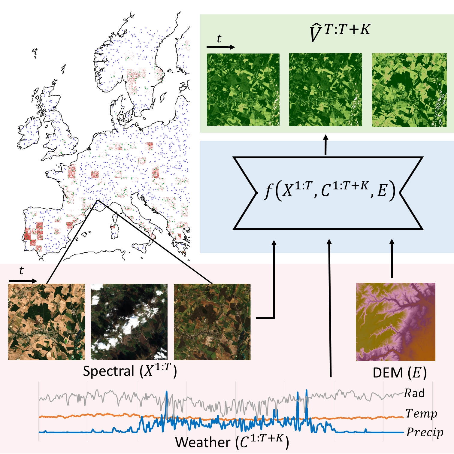
Figure 1: In this work, future vegetation status $\hat{V}$ is predicted with deep learning models $f$ from past satellite imagery $X$, past and future weather $C$ and elevation $E$. The underlying dataset spans across Europe with minicubes split into train (red dots), temporal OOD test (ood-t, orange dots) and spatio-temporal OOD test (ood-st, blue dots) subsets.

1 Introduction

Optical satellite images have been proven to be useful for monitoring vegetation status. This is necessary for a variety of applications in agriculture, forestry, humanitarian aid or carbon accounting. In all these cases, prognostic information is relevant: Farmers want to know how their farmland may react to a given weather scenario [58]. Humanitarian organisations need to understand the localized impact of droughts on pastoral communities for mitigation of famine with anticipatory action [32]. Afforestation efforts need to consider how their forests react to future climate [52].

However, such prognostic information is often not available at fine resolution. Even near-realtime data, is often still lacking. For instance in cloudy regions multiple weeks may pass before a clear-sky observation is available.

Forecasting optical satellite imagery as a way to tackle both issues has recently been investigated with video prediction methods [10, 23, 43, 45] on the EarthNet2021 dataset [43]. These models are able to forecast satellite imagery of high perceptual quality. However, their skill at modeling vegetation dynamics is harder to assess: despite EarthNet2021 being the largest such dataset for high resolution landscape forecasting [61], a faulty cloud mask, insufficient baselines and a poorly interpretable evaluation protocol still limit suitability of the EarthNet2021 dataset for vegetation prediction.

In this paper, we approach continental-scale modeling of vegetation dynamics. To achieve this, we predict remotely sensed vegetation greenness at 20m conditioned on coarse-scale weather. We extend the EarthNet2021 dataset [43] to be suitable for the task by improving cloud mask and spatio-temporal test sets. We then extend state-of-the-art approaches for video prediction with weather conditioning. Fig. 1 presents a sketch of our approach: Future vegetation state ($\hat{V}$) is predicted from satellite image spectra ($X$), past and future weather data ($C$), and elevation information ($E$) via deep learning ($f$).

Our major contributions can be summarized as follows. (1) We expand the EarthNet2021 dataset with a learned cloud mask and a new evaluation scheme to be suitable for vegetation prediction. (2) We present State-of-the-Art models for vegetation prediction, outperforming the top-3 approaches on the EarthNet2021 challenge and multiple other strong baselines both qualitatively and quantitatively. (3) We show how our results can be applied for prognostic carbon monitoring in a real-world use case.

Find our source code at https://github.com/earthnet2021/earthnet-models-pytorch.

2 Related Work

Vegetation Modeling Vegetation modeling from remote sensing has a long tradition at coarse resolution, e.g. from the AVHRR or MODIS satellites [21, 25, 28, 66]. Since 2015, the Sentinel 2 satellites deliver imagery at high resolution (up to $10$m). Several studies have used this data for regional crop yield modeling [49, 12] and regional vegetation forecasting [14, 64]. With EarthNet2021 [43], the first dataset for continental-scale satellite imagery forecasting was introduced. Subsequent works leveraged the ConvLSTM model [50] for satellite imagery prediction [10, 23] and for vegetation prediction in Africa [45]. Another line of work focuses on imputing cloudy time steps [31, 63], yet often with a focus on historical gapfilling instead of near-realtime information.

Spatio-temporal learning The ConvLSTM [50] was first introduced for precipitation nowcasting. Subsequently, spatio-temporal forecasting of the Earth system has gained traction, with strong results not only on precipitation nowcasting [42, 51], but also on weather forecasting [7, 26, 38], climate projection [35] and wildfire modeling [24]. Beyond the Earth system, video prediction is spatio-temporal learning. State-of-the-art video prediction models use ConvNets [4, 17], ConvLSTM successors [57, 59] or Transformers [18, 33]. A sub-area of video prediction uses action conditioning: predicting future frames by giving a future action in video games [36] or robot experiments [3, 15].

3 Methods

3.1 Task

We predict the future NDVI, a remote sensing proxy of vegetation state ($V^{t}\in\mathbb{R}^{H\times W},t\in[T+1,T+K]$) conditioned on past satellite imagery ($X^{t}\in\mathbb{R}^{H\times W},t\in[1,T]$), past and future weather ($C^{t}\in\mathbb{R},t\in[1,T+K]$) and static elevation maps ($E\in\mathbb{R}^{H\times W}$). Hence, denoting a model $f(.;\theta)$ with parameters $\theta$, we obtain vegetation predictions as:

$$\hat{V}^{T+1:T+K}=f(X^{1:T},C^{1:T+K},E;\theta)$$ (1)

In this paper most models are deep neural networks, trained with stochastic gradient descent to maximize a Gaussian Likelihood. More specifically, the optimal parameters $\theta^{*}$ are obtained by minimizing the mean squared error over valid pixels $V_{*}^{t}=V^{t}\odot M_{Q}^{t}\odot M_{L}$, where $M_{Q}\in\{0,1\}^{H\times W}$ masks pixels that are cloudy, cloud shadow or snow, $M_{L}\in\{0,1\}^{H\times W}$ masks pixels that are not cropland, forest, grassland or shrubland and $\odot$ denotes elementwise multiplication. Hence the training objective (leaving out dimensions for simplicity) is

$$\theta^{*}=\underset{\theta}{argmin}\frac{\sum(V-\hat{V})^{2}\odot M_{Q}\odot M_{L}}{\sum M_{Q}\odot M_{L}}$$ (2)

In this work $H=W=128\text{px},T=10$ and $K=20$.

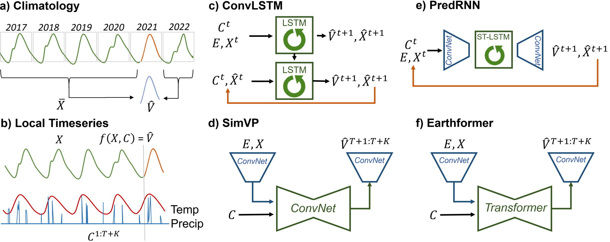
Figure 2: Simplified view of evaluated models. Baselines (a,b), weather-guided deep learning (c,d,e,f).

3.2 Models

This study focusses modeling around meteo-guided deep learning. We study in-depth four models which are representative for their respective model class. Two models perform next-frame prediction and leverage internal memory (ConvLSTM and PredRNN) to perform iterative roll-out. Two models perform next-cuboid prediction (SimVP and Earthformer), thereby modeling the full target period temporal dynamics at once. PredRNN, SimVP and Earthformer follow an encode-process-decode [6] configuration. Encoders and decoders operate in the spatial domain without any temporal fusion, while the processor translates latent features spatio-temporally. For encoding and decoding we leverage ConvNets, which are the standard in the domain of satellite remote sensing. The models are sketched in fig. 2 and described below.

ConvLSTM-meteo We follow the original ConvLSTM work [50] and use an encoding-forecasting setup (fig. 2c). It consists of two networks, each containing two ConvLSTM cells, without parameter sharing: One for the context period which works with past satellite imagery and past weather, and one for the target period, only using future weather as input. This is in contrast to the ConvLSTM flavors previously studied on EarthNet2021 [10, 23], but has been shown to work better on a similar problem in Africa [45].

PredRNN-meteo The PredRNN video prediction model [56, 57] is a ConvLSTM with two memory states: one for longer-term dynamics that passes information at the same depth level over time, and one for more complex short-term dynamics, with an information flow that zigzags through levels over time (called ST-LSTM). We propose a similar network to the action-conditioned PredRNN [57]: using ConvNet encoder and decoder and conditioning in each memory cell. We generalize their action-conditioning by using feature-wise linear modulation [39] for weather conditioning on the inputs (fig. 2e).

SimVP-meteo The SimVP video prediction model [54] is an encode-process-decode model with a ConvNet processor called Gated Spatiotemporal Attention Translator. It achieves temporal modeling by stacking the features of all time steps along the channel dimension. Each block then processes first with depth-wise convolution in the spatial domain, then with channel-wise convolutions in the temporal domain and finally gates with an attention layer. We achieve weather conditioning by feature-wise linear modulation [39] on the latent embeddings at each stage of the processor (fig. 2d).

Earthformer-meteo The Earthformer Earth system forecasting model [16] uses cuboid attention to process spatio-temporal chunks of information. It uses different cuboids of each input tensor as tokens for self- and cross-attention. Multiple cuboid attention modules are composed in a UNet like architecture. To tame the memory usage of the attention mechanisms, ConvNet encoder and decoder are used. Weather conditioning is achieved with early fusion during context steps and latent fusion during target steps (fig. 2f).

3.3 Baselines

We compare against several baselines:

Non-ML baselines We build three non-ML baselines. The persistence baseline, as in EarthNet2021 [43], constantly predicts the last valid NDVI observation from the context period. The previous year baseline [45] predicts the NDVI that was observed one year ago, obtained by interpolating last years observations linearly. The climatology baseline is produced by interpolating the NDVI timeseries leaving out the desired target year, then taking the mean over years, and then smoothing with a one month box-filter (fig. 2a).

Local timeseries models We compare against three commonly used time series models: Kalman filter, LightGBM [22] and Prophet [55] from the Python library darts [19]. These are trained on timeseries from a single pixel and applied to forecast this pixel, given future weather as covariates. Since they are fit for every pixel separately, running such timeseries models is expensive. Predicting a single minicube takes $\sim 3$h on an 8-CPU machine, which is $\mathcal{O}(10^{4})$ slower than the deep learning approaches.

LSTM A much faster timeseries model is the LSTM when trained globally. We implement a pixelwise LSTM as a ConvLSTM with 1x1 kernel size. It can not make use of spatial context, but does use temporal memory.

Next-frame UNet The next-frame UNet predicts autoregressively without memory the vegetation of the next time step. This is a common baseline for weather prediction, a task with insignificant memory effects [41].

Next-cuboid UNet The next-cuboid UNet works in chunks: It stacks all context time steps along the channel dimension and outputs all target time steps at once. It is similar to SimVP, but does early spatio-temporal fusion.

3.4 Implementation details

We build all of our ConvNets with a PatchMerge-style architecture similar to the one in Earthformer [16]. For SimVP and PredRNN, such encoders and decoders are more powerful, but also slightly more parameter-intensive, than the variants used in the original papers. We use GroupNorm [60] and LeakyReLU activation [62]. Skip connections preserve high-fidelity content between encoders and decoders. Our framework is implemented in PyTorch, and models are trained on Nvidia A40 and A100 GPUs. We use the AdamW [29] optimizer and tune the learning rate per model. More implementation details can be found in the supplementary materials.

Algorithm	Works on EN21	Prec	Rec	F1
Sen2Cor	Yes	0.83	0.60	0.70
FMask	No	0.85	0.85	0.85
KappaMask	No	0.74	0.88	0.81
UNet RGBNir	Yes	0.91	0.90	0.90
/w SCL	Yes	0.83	0.93	0.88
UNet 13Bands	No	0.94	0.92	0.93

Table 1: Precision, recall and F1-score of different Sentinel 2 cloud masking algorithms.

	Model	$R^{2}$ $\uparrow$	RMSE $\downarrow$	NSE $\uparrow$	$|\text{bias}|$ $\downarrow$	$\underset{\text{Climatology}}{\text{Outperform}}$ $\uparrow$	$\underset{25\text{ days}}{\text{RMSE}}$ $\downarrow$	#Params
non-ML	Persistence	0.00	0.23	-1.28	0.17	21.8%	0.09	0
	Previous year	0.56	0.20	-0.40	0.14	19.3%	0.18	0
	Climatology	0.58	0.18	-0.34	0.13	0.0%	0.16	0
black!30      local TS		Kalman filter	0.41	0.19	-0.57	0.13	27.0%	0.16	$\mathcal{O}$(10)
	LightGBM	0.51	0.17	-0.22	0.12	42.2%	0.11	n.a.
	Prophet	0.57	0.16	-0.05	0.11	60.6%	0.13	$\mathcal{O}$(10)
black!30      EN21		ConvLSTM [10]	0.51	0.18	-0.37	0.12	43.9%	0.12	0.2M
	SG-ConvLSTM [23]	0.53	0.19	-0.33	0.14	45.8%	0.11	0.7M
	Earthformer [16]	0.49	0.17	-0.27	0.12	47.2%	0.11	60.6M
black!30      This Study		ConvLSTM-meteo	0.62 $\pm$0.01	0.14 $\pm$0.00	0.11 $\pm$0.03	0.10 $\pm$0.00	68.2% $\pm$1.8%	0.10 $\pm$0.00	1.0M
	PredRNN-meteo	0.62 $\pm$0.00	0.15 $\pm$0.00	0.03 $\pm$0.00	0.10 $\pm$0.00	64.7% $\pm$1.2%	0.10 $\pm$0.00	1.4M
	SimVP-meteo	0.60 $\pm$0.00	0.15 $\pm$0.00	0.03 $\pm$0.01	0.09 $\pm$0.00	64.1% $\pm$1.0%	0.10 $\pm$0.00	6.6M
	Earthformer-meteo	0.52	0.16	-0.13	0.10	56.5%	0.09	60.6M
black

Table 2: Quantitative Results. For ConvLSTM-meteo, PredRNN-meteo and SimVP-meteo, we report the mean ($\pm$std. dev.) from three different random seeds.

3.5 Data

EarthNet2021 [43] is a dataset for Earth surface forecasting, that is weather-conditioned satellite image prediction. It contains spatio-temporal minicubes, that are a collection of $30$ 5-daily satellite images ($10$ context, $20$ target), $150$ daily meteorological observations and an elevation map. Spatial dimensions are $128\times 128$px ($2.56\times 2.56$km). We make the dataset suitable for vegetation modeling:

Cloud mask Vegetation proxies derived from optical satellite imagery are only meaningful if observations with clouds, shadows and snow are excluded. The cloudmask in EarthNet2021 is faulty. We train a UNet with Mobilenetv2 encoder [48] on the CloudSEN12 dataset [2] to detect clouds and cloud shadows from RGB and Nir bands. Tab. 1 compares precision, recall and F1 scores of detecting faulty pixels. Our approach outperforms Sen2Cor [30] (used in EarthNet2021), FMask [40] and KappaMask [11] baselines by a large margin. If using the Sentinel 2 SCL band in addition, to allow for snow masking, precision drops, but recall increases: i.e. the cloud mask gets more conservative. Using all 13 Sentinel 2 L2A bands is better than just using 4 bands, however such a model would not be directly applicable on EarthNet2021 data.

Test sets EarthNet2021 comes with four test sets. Yet, all of them contain data during the same period as training data, only at different locations (with varying degree of separation). Since weather has high spatial correlation lengths, model performance might be overestimated by evaluating at similar times but different locations. To tackle this, we introduce four new test sets and a new validation set:

• OOD-t contains 245 minicubes from the EarthNet2021 IID testset, stratified by Sentinel 2 tile, years 2021-2022

• val contains 245 minicubes from the EarthNet2021 IID testset, stratified by Sentinel 2 tile, year 2020

• OOD-s contains 800 minicubes stratified over $1\degree\times 1\degree$ lat-lon grid cells outside EarthNet2021 train regions, years 2017-2019

• OOD-st contains 800 minicubes stratified over $1\degree\times 1\degree$ lat-lon grid cells outside EarthNet2021 train regions, for the years 2021-2022

OOD-t is the main test set used throughout this study. It tests the models’ ability to extrapolate in time: i.e. we allow it to learn from past information about a location and want to know how it would perform in the future. val follows the same reasoning and hence allows for early stopping of models according to their temporal extrapolation skill. OOD-s and OOD-st test spatial extrapolation, as well as spatio-temporal extrapolation. For all test sets, we create minicubes over four periods during the European growing season [47] each year: Predicting March-May (MAM), May-July (MJJ), July-September (JAS) and September-November (SON).

Additional Layers We add the ESA Worldcover Landcover map [65] for selecting only vegetated pixels during evaluation, the Geomorpho90m Geomorphons map [1] for further evaluation and the ALOS [53], Copernicus [13] and NASA [9] DEMs, to provide uncertainty in the elevation maps. Furthermore, we update meteorology to a newer version of E-OBS [8], now containing the additional meteorological drivers wind speed, relative Humidity and shortwave downwelling radiation alongside the previously existing rainfall, sea-level pressure and temperature (daily mean, min & max). In contrast to EarthNet2021, we only provide one vector instead of a 3D tensor of meteorology, dropping the meso-scale surrounding of each minicube. This reduced the memory footprint of each minicube by $>5x$ and makes the task easier. Finally, we provide proper georeferencing, which was missing in EarthNet2021.

3.6 Evaluation

We resort to traditional metrics in environmental modeling:

• $R^{2}$ squared pearson correlation coefficient

• RMSE root mean squared error

• $\text{NSE}=1-\dfrac{MSE(V,\hat{V})}{Var[V]}$, the nash-sutcliffe efficiency [34], a measure of relative variability

• $|\text{bias}|=|\overline{V}-\overline{\hat{V}}|$, the absolute bias

In addition, we propose to measure if a model is better than the NDVI climatology, by computing the Outperformance score: The percentage of minicubes, for which the model is better in at least 3 out of the 4 metrics. Here, better means their score difference (ordering s.t. higher=better) exceeds $0.01$ for RMSE and $|\text{bias}|$ and $0.05$ for NSE and $R^{2}$. We also report the RMSE over only the first 25 days (5 time steps) of the target period.

We compute all metrics per pixel over clear-sky timesteps. We then consider only pixels with vegetated landcover (cropland, grassland, forest, shrubland), no seasonal flooding (minimum NDVI $>0$), enough observations ($\geq 10$ during target period, $\geq 3$ during context period) and considerable variation (NDVI std. dev $>0.1$). All these pixelwise scores are grouped by minicube and landcover, and then aggregated to account for class imbalance. Finally, the macro-average of the scores per landcover class is computed. In this way, the scores represent a conservative estimate of the expected performance of dynamic vegetation modeling during a new year or at a new location.

4 Experiments

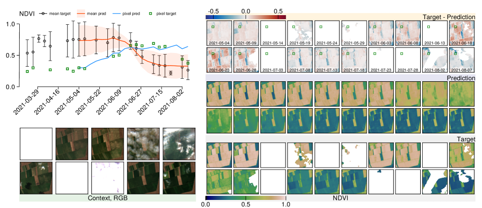
Figure 3: Qualitative Results. We plot results of PredRNN-meteo for one OOD-t minicube located near Oradea, Romania. The top-left shows timeseries for all pixels (mean and std. dev.) and for a single pixel (green square on top right). The right side shows image timeseries of cloud-masked target and predicted NDVI alongside their difference.

4.1 Baseline comparison

This work is the first to systematically evaluate vegetation prediction models at $20m$ resolution in Europe. However, previous work on satellite imagery forecasting is applicable, since the NDVI, our vegetation proxy, can be derived from the red and near-infrared channels. Hence, we evaluate the Top-3 models from the EarthNet2021 challenge leaderboard using their trained weights: a regular ConvLSTM [10], an encode-process-decode ConvLSTM called SGED-ConvLSTM [23] and the Earthformer [16].

We compare these against three Non-ML baselines: persistence, previous year and climatology. Note, the climatology uses a lot more information than our models (6 years vs. 50 days). Additionally, we compare with Kalman filter, LightGBM [22] and Prophet [55], local timeseries forecasting models, which also work with the full timeseries instead of just 50 context days.

We introduce four new model variants: ConvLSTM-meteo, PredRNN-meteo, SimVP-meteo and Earthformer-meteo (see sec. 3.2). These are weather-guided extensions of four state-of-the-art approaches to video prediction, each belonging to a different model class. For ConvLSTM-meteo, PredRNN-meteo and SimVP-meteo, we report the mean ($\pm$std. dev.) from three different random seeds. Earthformer-meteo has an order of magnitude more parameters, making training more expensive, which is why we only report one random seed.

The quantitative results are shown in table 3.4. Both the climatology and Prophet are strong baselines, which outperform all of the top-3 models from the EarthNet2021 challenge. SimVP, PredRNN and ConvLSTM outperform all baselines on all metrics except for the 25-day RMSE, where a persistence baseline is slightly stronger. For all three models and metrics, differences to the climatology are highly significant when tested for all pixels (with Wilcoxon signed-rank test, $\alpha=0.001$), but also for each land cover or for smaller subsets of $100$ minicubes. Earthformer-meteo, has overall lower skill. It mostly excels at RMSE and $|\text{bias}|$, where it can perform similar to other methods, yet has way lower performance for NSE and $R^{2}$. Here, NSE may be weak and RMSE good because we aggregate over the full dataset, hence indicating spatial patterns of model skill.

Qualitative results of the PredRNN model for one of the minicubes from the OOD-t test set with the highest scores are reported in fig. 3. The model clearly learns the complex dynamics of vegetation, with a strong seasonal evolution of the crop fields. It interpolates faithfully those pixels, which are masked in the target, and contains a strong temporal consistency. However, as the prediction horizon increases, predictions become more blurry, even obscuring field boundaries, which should stay consistent over time.

4.2 Weather guidance

Our meteo-guided models benefit from the weather conditioning. Fig. 4 compares each one of the four models (blue) against a variant without weather conditioning (orange). For all metrics (except Earthformer-meteo $R^{2}$), using weather outperforms not using it. The SimVP has the largest performance gain due to meteo-guidance. This could possibly be since it does not explicitly model memory effects, but rather learns to disentangle the temporal evolution in one piece. The ConvLSTM without weather has only slightly lower skill than the SimVP-meteo.

For PredRNN and SimVP, we perform an extended ablation study regarding weather guidance, which we present in the supplementary material. The different weather conditioning approaches concatenation, feature-wise linear modulation (FiLM, [39]) and cross-attention [46] have only a small influence on performance scores, if applied at the right location: cross-attention favors latent fusion, FiLM generally outperforms concatenation and is suitable for early fusion.

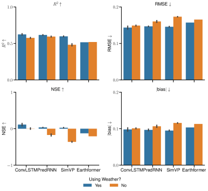
Figure 4: Model performance comparing meteo-guided models (blue) with the same those not using weather (black bar is std. dev. from three random seeds).

Acknowledgments. We are thankful for invaluable help, comments and discussions to Nuno Carvalhais, Reda ElGhawi, Christian Reimers, Annu Panwar and Xingjian Shi. MW thanks the European Space Agency for funding the project DeepExtremes (AI4Science ITT). CRM and LA are thankful to the European Union’s DeepCube Horizon 2020 (research and innovation programme grant agreement No 101004188). NL and JC acknowledge funding from the European Union’s Horizon 2020 research and innovation programme under grant agreement No 101003469.

Appendix A Model details

A.1 Cloud masking

Baselines (Table 1)

The baselines reported in table 1 are taken from CloudSEN12 [2]. Sen2Cor [30] is the processing software from ESA used to produce the Scene Classification Layer (SCL) mask, which was also introduced in EarthNet2021 [43]. FMask [40] is a processing software originally designed for NASA Landsat imagery, but now repurposed to also work with Sentinel 2 imagery. It requires L1C top-of-atmosphere reflectance from all bands to be produced (EarthNet2021 only containes L2A bottom-of-atmosphere reflectance from four bands). KappaMask [11] is a cloud mask based on deep learning, in table 1 we reported scores from the L2A version, which uses all 13 L2A bands as input.

UNet Mobilenetv2 (Table 1)

Our UNet with Mobilenetv2 encoder [48] was trained in two variants, one with RGB and near-infrared bands of L2A imagery (i.e. works with EarthNet2021) and one with all 13 bands of L2A imagery. We adopted the exact same implementation that was benchmarked in the CloudSEN12 paper [2], with the only difference being that in the paper, L1C imagery was used (which is often not useful in practical use-cases). In detail, this means we trained the UNet with Mobilenetv2 encoder using the Segmentation Models PyTorch Python library. We used a batch size of 32, random horizontal and vertical flipping, random 90 degree rotations, random mirroring, unweighted cross entropy loss, early stopping with a patience of 10 epochs, AdamW optimizer, learning rate of $1e^{-3}$, and a learning rate schedule reducing the learning rate by a factor of 10 if validation loss did not decrease for 4 epochs.

A.2 Vegetation modeling

Local timeseries models (Table 2)

We train the local timeseries models (table 2) at each pixel. For a given pixel we extract the full timeseries of NDVI and weather variables at 5-daily resolution. All variables are linearly gapfilled and weather is aggregated with min, mean, max, and std to 5-daily. The whole timeseries before each target period is used to train a timeseries model, for the target period the model only receives weather. The Kalman Filter runs with default parameters from darts [19]. The LightGBM model gets lagged variables from the last 10 time steps and predicts a full 20 time step chunk at once. For Prophet we again use default parameters.

EarthNet models (Table 2)

For running the leading models from EarthNet2021 we utilize the code from the respective github repositories: ConvLSTM [10], SGED-ConvLSTM [23] and Earthformer [16] . We derive the NDVI from the predicted satellite bands red and near-infrared:

$$NDVI=\frac{NIR-Red}{NIR+Red+1e^{-8}}$$ (3)

ConvLSTM-meteo (Table 2,3,4, Figure 4,5,6)

Our ConvLSTM-meteo contains four ConvLSTM-cells [50] in total, two for processing context frames and two for processing target frames. Each has convolution kernels with bias, hidden dimension of 64 and kernel size of 3. We train for 100 epochs with a batch size of 32, a learning rate of $4e^{-5}$ and with AdamW optimizer. We train three models from the random seeds 42, 97 and 27.

PredRNN-meteo (Table 2,3,4, Figure 3,4,7)

Our PredRNN-meteo contains two ST-ConvLSTM-cells [56] Each has convolution kernels with bias, hidden dimension of 64 and kernel size of 3 and residual connections. We use a PatchMerge encoder decoder with GroupNorm (16 groups), convolutions with kernel size of 3 and hidden dimension of 64, LeakyReLU activation and downsampling rate of 4x. We train for 100 epochs with a batch size of 32, a learning rate of $3e^{-4}$ and with AdamW optimizer. We use a spatio-temporal memory decoupling loss term with weight 0.1 and reverse exponential scheduling of true vs. predicted images (as in the PredRNN journal version [57]). We train three models from the random seeds 42, 97 and 27.

SimVP-meteo (Table 2,3,4, Figure 4)

Our SimVP-meteo has a PatchMerge encoder decoder with GroupNorm (16 groups), convolutions with kernel size of 3 and hidden dimension of 64, LeakyReLU activation and downsampling rate of 4x. The encoder processes all 10 context time steps at once (stacked along the channel dimension). The decoder processes 1 target time step at a time. The gated spatio-temporal attention processor [54] translates between both in the latent space, we use two layers and 64 hidden channels. We train for 100 epochs with a batch size of 64, a learning rate of $6e^{-4}$ and with AdamW optimizer. We train three models from the random seeds 42, 97 and 27.

Earthformer-meteo (Table 2,4, Figure 4)

Our Earthformer-meteo is a transformer combined with an initial PatchMerge encoder (and a final decoder) to reduce the dimensionality. The encoder and decoder use LeakyReLU activation, hidden size of 64 and 256 and downsample 2x. In between, the transformer processor has a UNet-type architecture, with cross-attention to merge context frame information with target frame embeddings. GeLU activation and LayerNorm, axial self-attention, 0.1 dropout and 4 attention heads are used. Weather information is regridded to match the spatial resolution of satellite imagery and used as input during context and target period. We train for 100 epochs with a batch size of 32, a maximum learning rate of $1e^{-4}$, linear learning rate warm up, cosine learning rate shedule and with AdamW optimizer.

1x1 LSTM (Table 4)

Our 1x1 LSTM is implemented as a ConvLSTM-meteo with kernel size of 1. We train for 100 epochs with a batch size of 32, a learning rate of $4e^{-5}$ and with AdamW optimizer.

Next-frame UNet (Table 4)

Our next-frame UNet has a depth of 5, latent weather conditioning with FiLM, a hidden size 128, kernel size 3, LeakyReLU activation, GroupNorm (16 groups), PatchMerge downsampling and nearest upsampling. We train for 100 epochs with a batch size of 64, a learning rate of $6e^{-4}$ and with AdamW optimizer.

Next-cuboid UNet (Table 4)

Our next-cuboid UNet has a depth of 5, latent weather conditioning with FiLM, a hidden size 256, kernel size 3, LeakyReLU activation, GroupNorm (16 groups), PatchMerge downsampling and nearest upsampling. We train for 100 epochs with a batch size of 64, a learning rate of $6e^{-4}$ and with AdamW optimizer.

Appendix B Weather ablations

B.1 Methods

Most of our baseline approaches have been originally proposed to handle only past covariates. Here, we condition forecasts on future weather. A-priori it is not known how to best achieve this weather conditioning. For PredRNN-meteo and SimVP-meteo, we compare three approaches, each fused at three different locations. The approaches operate pixelwise, taking features $x_{in}\in\mathbb{R}^{d}$ and conditioning input $c_{i}\in\mathbb{R}^{n}$ for weather variable $i$. The conditioning layers $g(\cdot,\cdot;\phi)$ with parameters $\phi$ then operate as

$$x_{out}=g(x_{in},c;\phi)\in\mathbb{R}^{d}$$ (4)

We parameterize $g$ with neural networks.

CAT

First concatenates $x_{in}$ and a flattened $c$ along the channel dimension, and then performs a linear projection to obtain $x_{out}$ of same dimensionality as $x_{in}$. In practice we implement this with a 1x1 Conv layer.

FiLM

Feature-wise linear modulation [39] generalizes the concatenation layer before. It produces $x_{out}$ with linear modulation:

$$x_{out}=x_{in}+\sigma(\gamma(c;\phi_{\gamma})\odot N(f(x_{in};\phi_{f}))+\beta(c;\phi_{\beta}))$$ (5)

Here, $f$ is a linear layer, $\gamma$ and $\beta$ are MLPs, $N$ is a normalization layer and $\sigma$ is a pointwise non-linear activation function.

xAttn

Cross-attention is an operation commonly found in the Transformers architecture. In recent works on image generation with diffusion models it is used to condition the generative process on a text embedding [46]. Inspired from this, we propose a pixelwise conditioning layer based on multi-head cross-attention. The input $x_{in}$ is treated as a single token query $Q$. Each weather variable $c_{i}$ is treated as individual tokens, from which we derive keys $K$ and values $V$. The result is then just regular multi-head attention $MHA$ in a residual block:

$$x_{out} =x_{in}$$ (6)

$$+f(N(MHA(Q(x_{in};\phi_{Q}),K(c;\phi_{K}),V(c;\phi_{V})));\phi_{f})$$ (7)

Here, $f$ is either a linear projection or a MLP and $N$ is a normalization layer.

Each of the three approaches we apply at three locations throughout the network:

Early fusion

Just fusing all data modalities before passing it to a model. This Early CAT has been previously used for weather conditioning in satellite imagery forecasting

Latent fusion

In the encode-process-decode framework, encoders are meant to capture spatial, and not temporal, relationships. Hence, latent fusion conditions the encoded spatial inputs twice: right after leaving the encoder and before entering the decoder.

All (fusion everywhere)

In addition, we compare against conditioning at every stage of the encoders, processors and decoders. All CAT has been applied to condition stochastic video predictions on random latent codes [27].

B.2 Results

Fig. 8 summarizes the findings by looking at the RMSE over the prediction horizon. For the first 50 days, most models are better than the climatology, afterwards, most are worse. If using early fusion, FiLM is the best conditioning method. For latent fusion and fusion everywhere (all), xAttn is a consistent choice, but FiLM may sometimes be better (and sometimes a lot worse). CAT in general should be avoided, which is consistent with the theoretical observation, that CAT is a special case of FiLM.

For SimVP, the best weather guiding method is latent fusion with FiLM. For PredRNN, the best method is early fusion with FiLM. This is likely due to the difference in treatment of the temporal axis. For SimVP, early fusion would merge all time steps, hence, latent fusion is a better choice. For PredRNN on the other hand, early fusion handles only a single timestep.

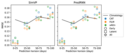
Figure 8: Model performance (RMSE) when using different ways of weather conditioning over varying prediction horizons.

Appendix C Performance per landcover type

Fig. 9 shows the model performance per landcover type.

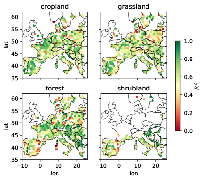
Figure 9: Model performance per landcover. Maps represent $R^{2}$ on OOD-t and OOD-st test sets of PredRNN-meteo.

References

- [1] Giuseppe Amatulli, Daniel McInerney, Tushar Sethi, Peter Strobl, and Sami Domisch. Geomorpho90m, empirical evaluation and accuracy assessment of global high-resolution geomorphometric layers. Scientific Data, 7(1):162, May 2020.
- [2] Cesar Aybar, Luis Ysuhuaylas, Jhomira Loja, Karen Gonzales, Fernando Herrera, Lesly Bautista, Roy Yali, Angie Flores, Lissette Diaz, Nicole Cuenca, Wendy Espinoza, Fernando Prudencio, Valeria Llactayo, David Montero, Martin Sudmanns, Dirk Tiede, Gonzalo Mateo-García, and Luis Gómez-Chova. CloudSEN12, a global dataset for semantic understanding of cloud and cloud shadow in Sentinel-2. Scientific Data, 9(1):782, Dec. 2022.
- [3] Mohammad Babaeizadeh, Chelsea Finn, Dumitru Erhan, Roy H. Campbell, and Sergey Levine. Stochastic Variational Video Prediction. In International Conference on Learning Representations, 2018.
- [4] Mohammad Babaeizadeh, Mohammad Taghi Saffar, Suraj Nair, Sergey Levine, Chelsea Finn, and Dumitru Erhan. FitVid: Overfitting in Pixel-Level Video Prediction, June 2021.
- [5] Shanning Bao, Andreas Ibrom, Georg Wohlfahrt, Sujan Koirala, Mirco Migliavacca, Qian Zhang, and Nuno Carvalhais. Narrow but robust advantages in two-big-leaf light use efficiency models over big-leaf light use efficiency models at ecosystem level. Agricultural and Forest Meteorology, 326:109185, Nov. 2022.
- [6] Peter W. Battaglia, Jessica B. Hamrick, Victor Bapst, Alvaro Sanchez-Gonzalez, Vinicius Zambaldi, Mateusz Malinowski, Andrea Tacchetti, David Raposo, Adam Santoro, Ryan Faulkner, Caglar Gulcehre, Francis Song, Andrew Ballard, Justin Gilmer, George Dahl, Ashish Vaswani, Kelsey Allen, Charles Nash, Victoria Langston, Chris Dyer, Nicolas Heess, Daan Wierstra, Pushmeet Kohli, Matt Botvinick, Oriol Vinyals, Yujia Li, and Razvan Pascanu. Relational inductive biases, deep learning, and graph networks, Oct. 2018.
- [7] Kaifeng Bi, Lingxi Xie, Hengheng Zhang, Xin Chen, Xiaotao Gu, and Qi Tian. Pangu-Weather: A 3D High-Resolution Model for Fast and Accurate Global Weather Forecast, Nov. 2022.
- [8] Richard C. Cornes, Gerard van der Schrier, Else J. M. van den Besselaar, and Philip D. Jones. An Ensemble Version of the E-OBS Temperature and Precipitation Data Sets. Journal of Geophysical Research: Atmospheres, 123(17):9391–9409, 2018.
- [9] R. Crippen, S. Buckley, P. Agram, E. Belz, E. Gurrola, S. Hensley, M. Kobrick, M. Lavalle, J. Martin, M. Neumann, Q. Nguyen, P. Rosen, J. Shimada, M. Simard, and W. Tung. NASADEM global elevation model: Methods and progress. In The International Archives of the Photogrammetry, Remote Sensing and Spatial Information Sciences, volume XLI-B4, pages 125–128. Copernicus GmbH, June 2016.
- [10] Codruț-Andrei Diaconu, Sudipan Saha, Stephan Günnemann, and Xiao Xiang Zhu. Understanding the Role of Weather Data for Earth Surface Forecasting Using a ConvLSTM-Based Model. In Proceedings of the IEEE/CVF Conference on Computer Vision and Pattern Recognition, pages 1362–1371, 2022.
- [11] Marharyta Domnich, Indrek Sünter, Heido Trofimov, Olga Wold, Fariha Harun, Anton Kostiukhin, Mihkel Järveoja, Mihkel Veske, Tanel Tamm, Kaupo Voormansik, Aire Olesk, Valentina Boccia, Nicolas Longepe, and Enrico Giuseppe Cadau. KappaMask: AI-Based Cloudmask Processor for Sentinel-2. Remote Sensing, 13(20):4100, Jan. 2021.
- [12] Martin Engen, Erik Sandø, Benjamin Lucas Oscar Sjølander, Simon Arenberg, Rashmi Gupta, and Morten Goodwin. Farm-Scale Crop Yield Prediction from Multi-Temporal Data Using Deep Hybrid Neural Networks. Agronomy, 11(12):2576, Dec. 2021.
- [13] ESA. Copernicus DEM - Global and European Digital Elevation Model (COP-DEM), 2021.
- [14] Aya Ferchichi, Ali Ben Abbes, Vincent Barra, and Imed Riadh Farah. Forecasting vegetation indices from spatio-temporal remotely sensed data using deep learning-based approaches: A systematic literature review. Ecological Informatics, page 101552, Jan. 2022.
- [15] Chelsea Finn, Ian Goodfellow, and Sergey Levine. Unsupervised Learning for Physical Interaction through Video Prediction. In Advances in Neural Information Processing Systems, volume 29. Curran Associates, Inc., 2016.
- [16] Zhihan Gao, Xingjian Shi, Hao Wang, Yi Zhu, Bernie Wang, Mu Li, and Dit-Yan Yeung. Earthformer: Exploring Space-Time Transformers for Earth System Forecasting. In Advances in Neural Information Processing Systems, Oct. 2022.
- [17] Zhangyang Gao, Cheng Tan, Lirong Wu, and Stan Z. Li. SimVP: Simpler Yet Better Video Prediction. In Proceedings of the IEEE/CVF Conference on Computer Vision and Pattern Recognition, pages 3170–3180, 2022.
- [18] Agrim Gupta, Stephen Tian, Yunzhi Zhang, Jiajun Wu, Roberto Martín-Martín, and Li Fei-Fei. MaskViT: Masked Visual Pre-Training for Video Prediction, Aug. 2022.
- [19] Julien Herzen, Francesco Lässig, Samuele Giuliano Piazzetta, Thomas Neuer, Léo Tafti, Guillaume Raille, Tomas Van Pottelbergh, Marek Pasieka, Andrzej Skrodzki, Nicolas Huguenin, Maxime Dumonal, Jan Kościsz, Dennis Bader, Frédérick Gusset, Mounir Benheddi, Camila Williamson, Michal Kosinski, Matej Petrik, and Gaël Grosch. Darts: User-Friendly Modern Machine Learning for Time Series. Journal of Machine Learning Research, 23(124):1–6, 2022.
- [20] ICOS RI. Ecosystem final quality (l2) product in etc-archive format - release 2022-1. station de-gri, 2022.
- [21] Lei Ji and A.J. Peters. Forecasting vegetation greenness with satellite and climate data. IEEE Geoscience and Remote Sensing Letters, 1(1):3–6, Jan. 2004.
- [22] Guolin Ke, Qi Meng, Thomas Finley, Taifeng Wang, Wei Chen, Weidong Ma, Qiwei Ye, and Tie-Yan Liu. LightGBM: A Highly Efficient Gradient Boosting Decision Tree. In Advances in Neural Information Processing Systems, volume 30. Curran Associates, Inc., 2017.
- [23] Klaus-Rudolf Kladny, Marco Milanta, Oto Mraz, Koen Hufkens, and Benjamin D. Stocker. Deep learning for satellite image forecasting of vegetation greenness. Preprint, Plant Biology, Aug. 2022.
- [24] Spyros Kondylatos, Ioannis Prapas, Michele Ronco, Ioannis Papoutsis, Gustau Camps-Valls, María Piles, Miguel-Ángel Fernández-Torres, and Nuno Carvalhais. Wildfire Danger Prediction and Understanding With Deep Learning. Geophysical Research Letters, 49(17):e2022GL099368, 2022.
- [25] Basil Kraft, Martin Jung, Marco Körner, Christian Requena Mesa, José Cortés, and Markus Reichstein. Identifying Dynamic Memory Effects on Vegetation State Using Recurrent Neural Networks. Frontiers in Big Data, 2, 2019.
- [26] Remi Lam, Alvaro Sanchez-Gonzalez, Matthew Willson, Peter Wirnsberger, Meire Fortunato, Alexander Pritzel, Suman Ravuri, Timo Ewalds, Ferran Alet, Zach Eaton-Rosen, Weihua Hu, Alexander Merose, Stephan Hoyer, George Holland, Jacklynn Stott, Oriol Vinyals, Shakir Mohamed, and Peter Battaglia. GraphCast: Learning skillful medium-range global weather forecasting, Dec. 2022.
- [27] Alex X. Lee, Richard Zhang, Frederik Ebert, Pieter Abbeel, Chelsea Finn, and Sergey Levine. Stochastic Adversarial Video Prediction, Apr. 2018.
- [28] Thomas Lees, Gabriel Tseng, Clement Atzberger, Steven Reece, and Simon Dadson. Deep Learning for Vegetation Health Forecasting: A Case Study in Kenya. Remote Sensing, 14(3):698, Jan. 2022.
- [29] Ilya Loshchilov and Frank Hutter. Decoupled Weight Decay Regularization. In International Conference on Learning Representations, Feb. 2022.
- [30] Jérôme Louis, Vincent Debaecker, Bringfried Pflug, Magdalena Main-Knorn, Jakub Bieniarz, Uwe Mueller-Wilm, Enrico Cadau, and Ferran Gascon. SENTINEL-2 SEN2COR: L2A Processor for Users. In L. Ouwehand, editor, Proceedings Living Planet Symposium 2016, volume SP-740, pages 1–8, Prague, Czech Republic, Aug. 2016. Spacebooks Online.
- [31] Andrea Meraner, Patrick Ebel, Xiao Xiang Zhu, and Michael Schmitt. Cloud removal in Sentinel-2 imagery using a deep residual neural network and SAR-optical data fusion. ISPRS Journal of Photogrammetry and Remote Sensing, 166:333–346, Aug. 2020.
- [32] Derege Tsegaye Meshesha, Muhyadin Mohammed Ahmed, Dahir Yosuf Abdi, and Nigussie Haregeweyn. Prediction of grass biomass from satellite imagery in Somali regional state, eastern Ethiopia. Heliyon, 6(10), Oct. 2020.
- [33] Charlie Nash, João Carreira, Jacob Walker, Iain Barr, Andrew Jaegle, Mateusz Malinowski, and Peter Battaglia. Transframer: Arbitrary Frame Prediction with Generative Models, May 2022.
- [34] J. E. Nash and J. V. Sutcliffe. River flow forecasting through conceptual models part I — A discussion of principles. Journal of Hydrology, 10(3):282–290, Apr. 1970.
- [35] Tung Nguyen, Johannes Brandstetter, Ashish Kapoor, Jayesh K. Gupta, and Aditya Grover. ClimaX: A foundation model for weather and climate, Jan. 2023.
- [36] Junhyuk Oh, Xiaoxiao Guo, Honglak Lee, Richard L Lewis, and Satinder Singh. Action-Conditional Video Prediction using Deep Networks in Atari Games. In Advances in Neural Information Processing Systems, volume 28. Curran Associates, Inc., 2015.
- [37] Daniel E. Pabon-Moreno, Mirco Migliavacca, Markus Reichstein, and Miguel D. Mahecha. On the potential of Sentinel-2 for estimating Gross Primary Production. IEEE Transactions on Geoscience and Remote Sensing, pages 1–1, 2022.
- [38] Jaideep Pathak, Shashank Subramanian, Peter Harrington, Sanjeev Raja, Ashesh Chattopadhyay, Morteza Mardani, Thorsten Kurth, David Hall, Zongyi Li, Kamyar Azizzadenesheli, Pedram Hassanzadeh, Karthik Kashinath, and Animashree Anandkumar. FourCastNet: A Global Data-driven High-resolution Weather Model using Adaptive Fourier Neural Operators, Feb. 2022.
- [39] Ethan Perez, Florian Strub, Harm de Vries, Vincent Dumoulin, and Aaron Courville. FiLM: Visual Reasoning with a General Conditioning Layer. Proceedings of the AAAI Conference on Artificial Intelligence, 32(1), Apr. 2018.
- [40] Shi Qiu, Zhe Zhu, and Binbin He. Fmask 4.0: Improved cloud and cloud shadow detection in Landsats 4–8 and Sentinel-2 imagery. Remote Sensing of Environment, 231:111205, Sept. 2019.
- [41] Stephan Rasp, Peter D. Dueben, Sebastian Scher, Jonathan A. Weyn, Soukayna Mouatadid, and Nils Thuerey. WeatherBench: A Benchmark Data Set for Data-Driven Weather Forecasting. Journal of Advances in Modeling Earth Systems, 12(11):e2020MS002203, 2020.
- [42] Suman Ravuri, Karel Lenc, Matthew Willson, Dmitry Kangin, Remi Lam, Piotr Mirowski, Megan Fitzsimons, Maria Athanassiadou, Sheleem Kashem, Sam Madge, Rachel Prudden, Amol Mandhane, Aidan Clark, Andrew Brock, Karen Simonyan, Raia Hadsell, Niall Robinson, Ellen Clancy, Alberto Arribas, and Shakir Mohamed. Skilful precipitation nowcasting using deep generative models of radar. Nature, 597(7878):672–677, Sept. 2021.
- [43] Christian Requena-Mesa, Vitus Benson, Markus Reichstein, Jakob Runge, and Joachim Denzler. EarthNet2021: A large-scale dataset and challenge for Earth surface forecasting as a guided video prediction task. In 2021 IEEE/CVF Conference on Computer Vision and Pattern Recognition Workshops (CVPRW), pages 1132–1142, June 2021.
- [44] Christian Requena-Mesa, Markus Reichstein, Miguel Mahecha, Basil Kraft, and Joachim Denzler. Predicting Landscapes from Environmental Conditions Using Generative Networks. In Gernot A. Fink, Simone Frintrop, and Xiaoyi Jiang, editors, Pattern Recognition, Lecture Notes in Computer Science, pages 203–217, Cham, 2019. Springer International Publishing.
- [45] Claire Robin, Christian Requena-Mesa, Vitus Benson, Lazaro Alonso, Jeran Poehls, Nuno Carvalhais, and Markus Reichstein. Learning to forecast vegetation greenness at fine resolution over Africa with ConvLSTMs, Nov. 2022.
- [46] Robin Rombach, Andreas Blattmann, Dominik Lorenz, Patrick Esser, and Björn Ommer. High-Resolution Image Synthesis With Latent Diffusion Models. In Proceedings of the IEEE/CVF Conference on Computer Vision and Pattern Recognition, pages 10684–10695, 2022.
- [47] Thomas Rötzer and Frank-M. Chmielewski. Phenological maps of Europe. Climate Research, 18(3):249–257, Nov. 2001.
- [48] Mark Sandler, Andrew Howard, Menglong Zhu, Andrey Zhmoginov, and Liang-Chieh Chen. MobileNetV2: Inverted Residuals and Linear Bottlenecks. In Proceedings of the IEEE Conference on Computer Vision and Pattern Recognition, pages 4510–4520, 2018.
- [49] Rai A. Schwalbert, Telmo J. C. Amado, Luciana Nieto, Sebastian Varela, Geomar M. Corassa, Tiago A. N. Horbe, Charles W. Rice, Nahuel R. Peralta, and Ignacio A. Ciampitti. Forecasting maize yield at field scale based on high-resolution satellite imagery. Biosystems Engineering, 171:179–192, July 2018.
- [50] Xingjian Shi, Zhourong Chen, Hao Wang, Dit-Yan Yeung, Wai-kin Wong, and Wang-chun WOO. Convolutional LSTM Network: A Machine Learning Approach for Precipitation Nowcasting. In Advances in Neural Information Processing Systems, volume 28. Curran Associates, Inc., 2015.
- [51] Xingjian Shi, Zhihan Gao, Leonard Lausen, Hao Wang, Dit-Yan Yeung, Wai-kin Wong, and Wang-chun WOO. Deep Learning for Precipitation Nowcasting: A Benchmark and A New Model. In Advances in Neural Information Processing Systems, volume 30. Curran Associates, Inc., 2017.
- [52] Joan Sturm, Maria J. Santos, Bernhard Schmid, and Alexander Damm. Satellite data reveal differential responses of Swiss forests to unprecedented 2018 drought. Global Change Biology, 28(9):2956–2978, 2022.
- [53] T. Tadono, H. Nagai, H. Ishida, F. Oda, S. Naito, K. Minakawa, and H. Iwamoto. Generation of the 30 m mesh global digital surface model by ALOS Prism. ISPRS - International Archives of the Photogrammetry, Remote Sensing and Spatial Information Sciences, XLI-B4:157–162, June 2016.
- [54] Cheng Tan, Zhangyang Gao, and Stan Z. Li. SimVP: Towards Simple yet Powerful Spatiotemporal Predictive Learning, Jan. 2023.
- [55] Sean J. Taylor and Benjamin Letham. Forecasting at Scale. The American Statistician, 72(1):37–45, Jan. 2018.
- [56] Yunbo Wang, Mingsheng Long, Jianmin Wang, Zhifeng Gao, and Philip S Yu. PredRNN: Recurrent Neural Networks for Predictive Learning using Spatiotemporal LSTMs. In Advances in Neural Information Processing Systems, volume 30. Curran Associates, Inc., 2017.
- [57] Yunbo Wang, Haixu Wu, Jianjin Zhang, Zhifeng Gao, Jianmin Wang, Philip S. Yu, and Mingsheng Long. PredRNN: A Recurrent Neural Network for Spatiotemporal Predictive Learning. IEEE Transactions on Pattern Analysis and Machine Intelligence, 45(2):2208–2225, Feb. 2023.
- [58] Aleksandra Wolanin, Gustau Camps-Valls, Luis Gómez-Chova, Gonzalo Mateo-García, Christiaan van der Tol, Yongguang Zhang, and Luis Guanter. Estimating crop primary productivity with Sentinel-2 and Landsat 8 using machine learning methods trained with radiative transfer simulations. Remote Sensing of Environment, 225:441–457, May 2019.
- [59] Haixu Wu, Zhiyu Yao, Jianmin Wang, and Mingsheng Long. MotionRNN: A Flexible Model for Video Prediction With Spacetime-Varying Motions. In Proceedings of the IEEE/CVF Conference on Computer Vision and Pattern Recognition, pages 15435–15444, 2021.
- [60] Yuxin Wu and Kaiming He. Group Normalization. In Proceedings of the European Conference on Computer Vision (ECCV), pages 3–19, 2018.
- [61] Zhitong Xiong, Fahong Zhang, Yi Wang, Yilei Shi, and Xiao Xiang Zhu. EarthNets: Empowering AI in Earth Observation, Dec. 2022.
- [62] Bing Xu, Naiyan Wang, Tianqi Chen, and Mu Li. Empirical Evaluation of Rectified Activations in Convolutional Network, Nov. 2015.
- [63] Xian Yang, Yifan Zhao, and Ranga Raju Vatsavai. Deep Residual Network with Multi-Image Attention for Imputing Under Clouds in Satellite Imagery. In 2022 26th International Conference on Pattern Recognition (ICPR), pages 643–649, Aug. 2022.
- [64] Wentao Yu, Jing Li, Qinhuo Liu, Jing Zhao, Yadong Dong, Cong Wang, Shangrong Lin, Xinran Zhu, and Hu Zhang. Spatial–Temporal Prediction of Vegetation Index With Deep Recurrent Neural Networks. IEEE Geoscience and Remote Sensing Letters, 19:1–5, 2022.
- [65] Daniele Zanaga, Ruben Van De Kerchove, Wanda De Keersmaecker, Niels Souverijns, Carsten Brockmann, Ralf Quast, Jan Wevers, Alex Grosu, Audrey Paccini, Sylvain Vergnaud, Oliver Cartus, Maurizio Santoro, Steffen Fritz, Ivelina Georgieva, Myroslava Lesiv, Sarah Carter, Martin Herold, Linlin Li, Tsendbazar, Nandin-Erdene, Fabrizio Ramoino, and Olivier Arino. ESA WorldCover 10 m 2020 v100, Oct. 2021.
- [66] Yelu Zeng, Dalei Hao, Alfredo Huete, Benjamin Dechant, Joe Berry, Jing M. Chen, Joanna Joiner, Christian Frankenberg, Ben Bond-Lamberty, Youngryel Ryu, Jingfeng Xiao, Ghassem R. Asrar, and Min Chen. Optical vegetation indices for monitoring terrestrial ecosystems globally. Nature Reviews Earth & Environment, pages 1–17, May 2022.