Symmetric Rank-$k$ Methods

Abstract

This paper proposes a novel class of block quasi-Newton methods for convex optimization which we call symmetric rank-$k$ (SR-$k$) methods. Each iteration of SR-$k$ incorporates the curvature information with $k$ Hessian-vector products achieved from the greedy or random strategy. We prove SR-$k$ methods have the local superlinear convergence rate of ${\mathcal{O}}\big{(}(1-k/d)^{t(t-1)/2}\big{)}$ for minimizing smooth and strongly convex function, where $d$ is the problem dimension and $t$ is the iteration counter. This is the first explicit superlinear convergence rate for block quasi-Newton methods, and it successfully explains why block quasi-Newton methods converge faster than ordinary quasi-Newton methods in practice.

1 Introduction

We study quasi-Newton methods for solving the minimization problem

$$\min_{{\bf x}\in{\mathbb{R}}^{d}}f({\bf x}),$$ (1)

where $f:{\mathbb{R}}^{d}\to{\mathbb{R}}$ is smooth and strongly convex. Quasi-Newton methods [5, 4, 37, 3, 9, 7, 40] are widely recognized for their fast convergence rates and efficient updates, which attracts growing attention in many fields such as statistics [17, 41, 2], economics [28, 23] and machine learning [13, 16, 25, 26, 22]. Unlike standard Newton methods which need to compute the Hessian and its inverse, quasi-Newton methods go along the descent direction by the following scheme

$${\bf x}_{t+1}={\bf x}_{t}-{\bf G}_{t}^{-1}\nabla f({\bf x}_{t}),$$

where ${\bf G}_{t}\in{\mathbb{R}}^{d\times d}$ is an estimator of the Hessian $\nabla^{2}f({\bf x}_{t})$. The most popular ways to construct the Hessian estimator are the Broyden family updates, including the Davidon–Fletcher–Powell (DFP) method [9, 11], the Broyden–Fletcher–Goldfarb–Shanno (BFGS) method [5, 4, 37], and the symmetric rank-one (SR1) method [3, 9].

The classical quasi-Newton methods with Broyden family updates [5, 4] find the Hessian estimator ${\bf G}_{t+1}$ for the next round by the secant equation

$${\bf G}_{t+1}({\bf x}_{t+1}-{\bf x}_{t})=\nabla f({\bf x}_{t+1})-\nabla f({\bf x}_{t}).$$ (2)

These methods have been proven to exhibit local superlinear convergence in 1970s [32, 10, 6], and their non-asymptotic superlinear rates were established in recent years [35, 34, 39, 19]. For example, Rodomanov and Nesterov [35] showed classical BFGS method enjoys the local superlinear rates of ${\mathcal{O}}\big{(}(d\varkappa/t)^{t/2}\big{)}$, where $\varkappa$ is the condition number of the objective. They also improved this result to ${\mathcal{O}}\big{(}(\exp{(d\ln(\varkappa)/t)}-1)^{t/2}\big{)}$ [34]. Later, Ye et al. [39] showed classical SR1 method converges with local superlinear rate of ${\mathcal{O}}\big{(}(d\ln(\varkappa)/t)^{t/2}\big{)}$.

Some recent works [14, 33] proposed another type of quasi-Newton methods, which construct the Hessian estimator by the following equation

$${\bf G}_{t+1}{\bf u}_{t}=\nabla^{2}f({\bf x}_{t+1}){\bf u}_{t},$$ (3)

where ${\bf u}_{t}\in{\mathbb{R}}^{d}$ is chosen by greedy or randomized strategies. Rodomanov and Nesterov [33] established the local superlinear rate of ${\mathcal{O}}\big{(}(1-{1}/{(\varkappa d)})^{t(t-1)/2}\big{)}$ for greedy quasi-Newton methods with Broyden family updates. Later, Lin et al. [24] provided the condition-number free superlinear rate of ${\mathcal{O}}\big{(}(1-{1}/{d})^{t(t-1)/2}\big{)}$ for greedy and randomized quasi-Newton methods with specific BFGS and SR1 updates.

Block quasi-Newton methods construct the Hessian estimator along multiple directions at per iteration. The study of these methods dates back to 1980s. Schnabel [36] proposed the first block BFGS method by extending equation (2) to multiple secant equations

$${\bf G}_{t+1}({\bf x}_{t+1}-{\bf x}_{t+1-j})=\nabla f({\bf x}_{t+1})-\nabla f({\bf x}_{t+1-j})$$

for $j=1,\dots,k$. Although block quasi-Newton methods usually have better empirical performance than ordinary quasi-Newton methods without block fashion updates [36, 31, 12, 15, 14, 21], their theoretical guarantees are mystery until Gao and Goldfarb [12] proved block BFGS method has asymptotic local superlinear convergence. On the other hand, Gower et al. [15], Gower and Richtárik [14], Kovalev et al. [21] introduced the randomized block BFGS by generalizing condition (3) to

$${\bf G}_{t+1}{\bf U}_{t}=\nabla^{2}f({\bf x}_{t+1}){\bf U}_{t},$$

where ${\bf U}_{t}\in{\mathbb{R}}^{d\times k}$ is some randomized matrix. Their empirical studies showed randomized block BFGS performs well on real-world applications. In addition, Kovalev et al. [21] proved randomized block BFGS method also has asymptotic local superlinear convergence, but its advantage over ordinary BFGS methods is still unclear in theory.

The theoretical results of existing block quasi-Newton methods cannot explain why they enjoy faster convergence behavior than ordinary quasi-Newton methods in practice. This naturally leads to the following question:

Can we provide a block quasi-Newton method with explicit superior convergence rate?

In this paper, we give an affirmative answer by proposing symmetric rank-$k$ (SR-$k$) methods. The constructions of Hessian estimators in SR-$k$ methods are based on generalizing the idea of symmetric rank-1 (SR1) [3, 9, 39] methods and the equation of the form (3). We provide the randomized and greedy strategies to determine ${\bf U}_{t}\in{\mathbb{R}}^{d\times k}$ for SR-$k$. Both of them lead to the explicit local superlinear convergence rate of ${\mathcal{O}}\big{(}(1-{k}/{d})^{t(t-1)/2}\big{)}$, where $k$ is the number of directions used to approximate Hessian at per iteration. For $k=1$, our methods reduce to randomized and greedy SR1 methods [24]. For $k\geq 2$, it is clear that SR-$k$ methods have faster superlinear rates than existing greedy and randomized quasi-Newton methods [24, 33]. We also follow the design of SR-$k$ to propose a variant of randomized block BFGS method [15, 14, 21] and a randomized block DFP method, resulting an explicit superlinear convergence rate of ${\mathcal{O}}\big{(}(1-k/(\varkappa d))^{t(t-1)/2}\big{)}$. We compare the results of proposed methods with existing quasi-Newton methods in Table 1.

The remainder of this paper is organized as follows. In Section 2, we introduce the notation and the preliminaries throughout this paper. In Section 3, we propose the SR-$k$ update in the view of matrix approximation. In Section 4, we propose the quasi-Newton methods with SR-$k$ updates for minimizing smooth and strongly convex function and provide their the superior local superlinear convergence rates. In Section 5, we propose a new randomized block BFGS method and randomized block DFP method with explicit local superlinear convergence rates. In Section 6, we conduct numerical experiments to show the outperformance of proposed methods. Finally, we conclude our work in Section 7.

Table 1: We summarize the local convergence rates of existing and proposed quasi-Newton methods for strongly convex optimization. The second column displays the rank of modification (i.e., ${\bf G}_{+}-{\bf G}$ in SR-$k$ update (7)-(8)) in per iteration of quasi-Newton methods.

Methods	Rank	Convergence	Reference
Newton Method	$d$	quadratic	[29, 30]
Classical BFGS/DFP	$2$	$\displaystyle{{\mathcal{O}}\big{(}\big{(}{d\varkappa}/{t}\big{)}^{t/2}\big{)}}$ $\displaystyle{{\mathcal{O}}\big{(}\big{(}\exp{({d\ln(\varkappa)}/{t})}-1\big{)}^{t/2}\big{)}}$ $\displaystyle{{\mathcal{O}}\big{(}\big{(}{1}/{t}\big{)}^{t/2}\big{)}}$ (*)	[35] [34] [19]
Classical SR1	$1$	$\displaystyle{{\mathcal{O}}\big{(}\big{(}{d\ln(\varkappa)}/{t}\big{)}^{t/2}\big{)}}$	[39]
Greedy/Randomized Broyden Family	$1$ or $2$	$\displaystyle{{\mathcal{O}}\big{(}(1-1/(\varkappa d))^{{t(t-1)}/{2}}\big{)}}$	[33, 24]
Greedy/Randomized BFGS	$2$	$\displaystyle{{\mathcal{O}}\big{(}(1-1/d)^{{t(t-1)}/{2}}\big{)}}$	[24]
Greedy/Randomized SR1	$1$	$\displaystyle{{\mathcal{O}}\big{(}(1-1/d)^{{t(t-1)}/{2}}\big{)}}$	[24]
Multi-Secant Block-BFGS	$k\in[d]$	asymptotic superlinear	[36, 12]
Randomized Block-BFGS (v1)	$k\in[d]$	asymptotic superlinear	[21, 14]
​​Randomized Block-BFGS (v2)	​$k\in[d]$	$\displaystyle{{\mathcal{O}}\big{(}(1-{k}/{(\varkappa d)})^{{t(t-1)}/{2}}\big{)}}$	Algorithm 3
Randomized Block-DFP	​$k\in[d]$	$\displaystyle{{\mathcal{O}}\big{(}(1-{k}/{(\varkappa d)})^{{t(t-1)}/{2}}\big{)}}$	Algorithm 3
Greedy/Randomized SR-$k$	$k\in[d-1]$  $k=d$	${\mathcal{O}}\left((1-{k}/{d})^{{t(t-1)}/{2}}\right)$ quadratic	Algorithm 1

• The convergence rate(s) require an additional assumption that the initial Hessian estimator be sufficiently closed to the true Hessian.

2 Preliminaries

We first introduce the notations used in this paper. We use $\{{\bf e}_{1},\cdots,{\bf e}_{d}\}$ to present the the standard basis in space ${\mathbb{R}}^{d}$ and let ${\bf I}_{d}\in{\mathbb{R}}^{d\times d}$ be the identity matrix. We use ${\bf S}^{{\dagger}}$ to denote the Moore-Penrose inverse of matrix ${\bf S}$. We denote the trace of a square matrix by ${\rm tr}\left(\cdot\right)$. We use $\|\cdot\|$ to present the spectral norm and Euclidean norm of matrix and vector respectively. Given a positive definite matrix ${\bf A}\in{\mathbb{R}}^{d\times d}$, we denote the corresponding weighted norm as $\|{{\bf x}}\|_{\bf A}\triangleq({{\bf x}}^{\top}{\bf A}{{\bf x}})^{1/2}$ for some ${{\bf x}}\in{\mathbb{R}}^{d}$. We use the notation $\left\|{{\bf x}}\right\|_{\bf{z}}$ to present $\|{{\bf x}}\|_{\nabla^{2}f({\bf{z}})}$ for positive definite Hessian $\nabla^{2}f({\bf{z}})$, if there is no ambiguity for the reference function $f(\cdot)$. We also define

$${\bf E}_{k}({\bf A})\triangleq[{\bf{e}}_{i_{1}};\cdots;{\bf{e}}_{i_{k}}]\in{\mathbb{R}}^{d\times k},$$ (4)

where $i_{1},\dots,i_{k}$ are the indices for the largest $k$ entries in the diagonal of ${\bf A}$.

Throughout this paper, we suppose the objective in problem (1) satisfies the following assumptions.

Assumption 2.1.

We assume the objective function $f:{\mathbb{R}}^{d}\to{\mathbb{R}}$ is $L$-smooth, i.e., there exists some constant $L\geq 0$ such that $\|\nabla f({{\bf x}})-\nabla f({{\bf y}})\|\leq L\|{{\bf x}}-{{\bf y}}\|$ for any ${{\bf x}},{{\bf y}}\in{\mathbb{R}}^{d}.$

Assumption 2.2.

We assume the objective function $f:{\mathbb{R}}^{d}\to{\mathbb{R}}$ is $\mu$-strongly-convex, i.e., there exists some constant $\mu>0$ such that

$$f(\lambda{{\bf x}}+(1-\lambda){{\bf y}})\leq\lambda f({{\bf x}})+(1-\lambda)f({{\bf y}})-\frac{\lambda(1-\lambda)\mu}{2}\left\|{{\bf x}}-{{\bf y}}\right\|_{2}^{2}$$

for any ${{\bf x}},{{\bf y}}\in{\mathbb{R}}^{d}$ and $\lambda\in[0,1]$.

We define the condition number as $\varkappa\triangleq L/\mu$. The following proposition shows the objective function has bounded Hessian under Assumption 2.1 and 2.2.

Proposition 2.3.

Suppose the objective function $f:{\mathbb{R}}^{d}\to{\mathbb{R}}$ satisfies Assumptions 2.1 and 2.2, then it holds

$$\mu{\bf I}_{d}\preceq\nabla^{2}f({\bf x})\preceq L{\bf I}_{d}$$ (5)

for any ${\bf x}\in{\mathbb{R}}^{d}$.

We also impose the assumption of strongly self-concordance [33, 24] as follows.

Assumption 2.4.

We assume the objective function $f:{\mathbb{R}}^{d}\to{\mathbb{R}}$ is $M$-strongly self-concordant, i.e., there exists some constant $M\geq 0$ such that

$$\nabla^{2}f({\bf y})-\nabla^{2}f({\bf x})\preceq M\|{\bf y}-{\bf x}\|_{\bf z}\nabla^{2}f({\bf w}),$$ (6)

for any ${\bf x},{\bf y},{\bf w},{\bf z}\in{\mathbb{R}}^{d}$.

The strongly-convex function with Lipschitz-continuous Hessian is strongly self-concordant.

Proposition 2.5.

Suppose the objective function $f:{\mathbb{R}}^{d}\to{\mathbb{R}}$ satisfies Assumptions 2.2 and its Hessian is $L_{2}$-Lipschitz continuous, i.e., we have

$$\|\nabla^{2}f({\bf x})-\nabla^{2}f({\bf y})\|\leq L_{2}\|{\bf x}-{\bf y}\|,$$

for all ${\bf x}$, ${\bf y}\in{\mathbb{R}}^{d}$, then the function $f(\cdot)$ is $M$-strongly self-concordant with $M={L_{2}}/{\mu^{3/2}}$.

3 Symmetric Rank-$k$ Updates

We propose the block version of classical SR1 update, called the symmetric rank-$k$ (SR-$k$) update, as follows.

Definition 3.1 (SR-$k$ Update).

Let ${\bf A}\in{\mathbb{R}}^{d\times d}$ and ${\bf G}\in{\mathbb{R}}^{d\times d}$ be two positive-definite matrices with ${\bf A}\preceq{\bf G}$. For any matrix ${\bf U}\in{\mathbb{R}}^{d\times k}$, we define

$${\text{SR-$k$}}({\bf G},{\bf A},{\bf U})\triangleq{\bf G}-({\bf G}-{\bf A}){\bf U}({\bf U}^{\top}({\bf G}-{\bf A}){\bf U})^{{\dagger}}{\bf U}^{\top}({\bf G}-{\bf A}).$$ (7)

In this section, we always use ${\bf G}_{+}$ to denote the output of SR-$k$ update such that

$${\bf G}_{+}\triangleq{\text{SR-$k$}}({\bf G},{\bf A},{\bf U}).$$ (8)

We provide the following lemma to show that SR-$k$ update does not increase the deviation from the target matrix ${\bf A}$, which is similar to ordinary Broyden family updates [33].

Lemma 3.2.

Given any positive-definite matrices ${\bf A}\in{\mathbb{R}}^{d\times d}$ and ${\bf G}\in{\mathbb{R}}^{d\times d}$ with ${\bf A}\preceq{\bf G}\preceq\eta{\bf A}$ for some $\eta\geq 1$, it holds that

$${\bf A}\preceq{\bf G}_{+}\preceq\eta{\bf A}.$$ (9)

Proof.

According to the update rule (7), we have

$${\bf G}_{+}-{\bf A}$$

$$=({\bf G}-{\bf A})-({\bf G}-{\bf A}){\bf U}({\bf U}^{\top}({\bf G}-{\bf A}){\bf U})^{{\dagger}}{\bf U}^{\top}({\bf G}-{\bf A})$$

$$=\left({\bf I}_{d}-({\bf G}-{\bf A}){\bf U}({\bf U}^{\top}({\bf G}-{\bf A}){\bf U})^{{\dagger}}{\bf U}^{\top}\right)({\bf G}-{\bf A})\left({\bf I}_{d}-{\bf U}({\bf U}^{\top}({\bf G}-{\bf A}){\bf U})^{{\dagger}}{\bf U}^{\top}({\bf G}-{\bf A})\right)\succeq{\bf 0},$$

which indicates ${\bf G}_{+}\succeq{\bf A}$. The condition ${\bf G}\preceq\eta{\bf A}$ means

$${\bf G}_{+} \preceq\eta{\bf A}-\underbrace{({\bf G}-{\bf A}){\bf U}({\bf U}^{\top}({\bf G}-{\bf A}){\bf U})^{{\dagger}}{\bf U}^{\top}({\bf G}-{\bf A})}_{\succeq{\bf 0}}\preceq\eta{\bf A},$$

which finish the proof. ∎

To evaluate the convergence of SR-$k$ update, we introduce the following quantity [24, 39]

$$\tau_{\bf A}({\bf G})\triangleq{\rm tr}\left({\bf G}-{\bf A}\right)$$ (10)

which characterizes the difference between target matrix ${\bf A}$ and the current estimator ${\bf G}$.

In the remainder of this section, we aim to establish the convergence guarantee

$${\mathbb{E}}\left[\tau_{{\bf A}}({\bf G}_{+})\right]\leq\left(1-\frac{k}{d}\right)\tau_{{\bf A}}({\bf G}),$$ (11)

for approximating the target matrix ${\bf A}$ by SR-$k$ iteration (8) with appropriate choice of ${\bf U}\in{\mathbb{R}}^{d\times k}$. Note that if we take $k=1$, the equation (11) will reduce to ${\mathbb{E}}\left[\tau_{{\bf A}}({\bf G}_{+})\right]\leq\left(1-{1}/{d}\right)\tau_{{\bf A}}({\bf G})$, which corresponds the convergence result of randomized and greedy SR1 updates [24].

Observe that we can split $\tau_{{\bf A}}({\bf G}_{+})$ as follows

$$\begin{split}\tau_{{\bf A}}({\bf G}_{+})&\!\overset{\eqref{eq:srk},\eqref{iter:srk}}{=}{\rm tr}\left({\bf G}-{\bf A}-({\bf G}-{\bf A}){\bf U}({\bf U}^{\top}({\bf G}-{\bf A}){\bf U})^{{\dagger}}{\bf U}^{\top}({\bf G}-{\bf A})\right)\\ &~{}~{}=\underbrace{{\rm tr}\left({\bf G}-{\bf A}\right)}_{\text{Part}~{}{\rm I}}-\underbrace{{\rm tr}\left(({\bf G}-{\bf A}){\bf U}({\bf U}^{\top}({\bf G}-{\bf A}){\bf U})^{{\dagger}}{\bf U}^{\top}({\bf G}-{\bf A})\right)}_{\text{Part}~{}{\rm II}},\end{split}$$ (12)

where Part I is equal to $\tau_{{\bf A}}({\bf G})$ and Part II encourage the SR-$k$ update to decrease $\tau_{\bf A}(\cdot)$. To obtain the desired result of (11), we only need to prove Part II satisfies

$${\mathbb{E}}\left[{\rm tr}\left(({\bf G}-{\bf A}){\bf U}({\bf U}^{\top}({\bf G}-{\bf A}){\bf U})^{{\dagger}}{\bf U}^{\top}({\bf G}-{\bf A})\right)\right]\geq\frac{k}{d}{\rm tr}\left({\bf G}-{\bf A}\right).$$

We first provide the following lemma to bound Part II (in the view of ${\bf R}={\bf G}-{\bf A}$).

Lemma 3.3.

For positive semi-definite matrix ${\bf R}\in{\mathbb{R}}^{d\times d}$ and full rank matrix ${\bf U}\in{\mathbb{R}}^{d\times k}$ with $k\leq d$, it holds that

$${\rm tr}\left({\bf R}{\bf U}\left({\bf U}^{\top}{\bf R}{\bf U}\right)^{{\dagger}}{\bf U}^{\top}{\bf R}\right)\geq{\rm tr}\left({\bf U}\left({\bf U}^{\top}{\bf U}\right)^{-1}{\bf U}^{\top}{\bf R}\right).$$ (13)

Proof.

Let ${\bf U}={\bf Q}{\bf\Sigma}{\bf V}^{\top}$ be SVD of ${\bf U}$, where ${\bf Q}\in{\mathbb{R}}^{d\times k}$, ${\bf V}\in{\mathbb{R}}^{k\times k}$ are (column) orthogonal and ${\bf\Sigma}\in{\mathbb{R}}^{k\times k}$ is diagonal, then the right-hand side of inequality (13) can be written as

$${\rm tr}\left({\bf U}\left({\bf U}^{\top}{\bf U}\right)^{-1}{\bf U}^{\top}{\bf R}\right) ={\rm tr}\left({\bf Q}{\bf\Sigma}{\bf V}^{\top}\left({\bf V}{\bf\Sigma}^{2}{\bf V}^{\top}\right)^{-1}{\bf V}{\bf\Sigma}{\bf Q}^{\top}{\bf R}\right)={\rm tr}\left({\bf Q}{\bf Q}^{\top}{\bf R}\right).$$

Consequently, we upper bound the left-hand side of inequality (13) as follows

$${\rm tr}\left({\bf R}{\bf U}\left({\bf U}^{\top}{\bf R}{\bf U}\right)^{{\dagger}}{\bf U}^{\top}{\bf R}\right)$$

$$={\rm tr}\left({\bf R}{\bf Q}{\bf\Sigma}{\bf V}^{\top}\left({\bf V}{\bf\Sigma}{\bf Q}^{\top}{\bf R}{\bf Q}{\bf\Sigma}{\bf V}^{\top}\right)^{{\dagger}}{\bf V}{\bf\Sigma}{\bf Q}^{\top}{\bf R}\right)$$

$$={\rm tr}\left({\bf R}{\bf Q}{\bf\Sigma}\left({\bf\Sigma}{\bf Q}^{\top}{\bf R}{\bf Q}{\bf\Sigma}\right)^{{\dagger}}{\bf\Sigma}{\bf Q}^{\top}{\bf R}\right)$$

$$={\rm tr}\left({\bf Q}^{\top}{\bf R}{\bf Q}{\bf\Sigma}\left({\bf\Sigma}{\bf Q}^{\top}{\bf R}{\bf Q}{\bf\Sigma}\right)^{{\dagger}}{\bf\Sigma}{\bf Q}^{\top}{\bf R}{\bf Q}\right)+{\rm tr}\left(({\bf I}_{d}-{\bf Q}{\bf Q}^{\top})^{1/2}{\bf R}{\bf Q}{\bf\Sigma}\left({\bf\Sigma}{\bf Q}^{\top}{\bf R}{\bf Q}{\bf\Sigma}\right)^{{\dagger}}{\bf\Sigma}{\bf Q}^{\top}{\bf R}({\bf I}_{d}-{\bf Q}{\bf Q}^{\top})^{1/2}\right)$$

$$\geq{\rm tr}\left({\bf Q}^{\top}{\bf R}{\bf Q}{\bf\Sigma}\left({\bf\Sigma}{\bf Q}^{\top}{\bf R}{\bf Q}{\bf\Sigma}\right)^{{\dagger}}{\bf\Sigma}{\bf Q}^{\top}{\bf R}{\bf Q}\right)$$

$$={\rm tr}\left({\bf\Sigma}^{-1}{\bf\Sigma}{\bf Q}^{\top}{\bf R}{\bf Q}{\bf\Sigma}\left({\bf\Sigma}{\bf Q}^{\top}{\bf R}{\bf Q}{\bf\Sigma}\right)^{{\dagger}}{\bf\Sigma}{\bf Q}^{\top}{\bf R}{\bf Q}{\bf\Sigma}{\bf\Sigma}^{-1}\right)$$

$$={\rm tr}\left({\bf\Sigma}^{-1}{\bf\Sigma}{\bf Q}^{\top}{\bf R}{\bf Q}{\bf\Sigma}{\bf\Sigma}^{-1}\right)$$

$$={\rm tr}\left({\bf Q}^{\top}{\bf R}{\bf Q}\right),$$

where the inequality is due to the fact that

$${\bf I}_{d}-{\bf Q}{\bf Q}^{\top}={\bf I}_{d}-{\bf Q}({\bf Q}^{\top}{\bf Q})^{-1}{\bf Q}^{\top}\succeq{\bf 0}.$$

Combining all above results leads to inequality (13). ∎

We then provide two strategies to select matrix ${\bf U}\in{\mathbb{R}}^{d\times k}$ for SR-$k$ update:

1. For randomized strategy, we sample each entry of ${\bf U}$ according to standard normal distribution independently, i.e.,

   $$[{\bf U}]_{ij}\overset{{\rm i.i.d}}{\sim}{\mathcal{N}}(0,1).$$

2. For greedy strategy, we construct ${\bf U}$ as

   $${\bf U}={\bf E}_{k}({\bf G}-{\bf A}),$$

   where ${\bf E}_{k}(\cdot)$ follows the notation of (4).

The following lemma indicates that the term of ${\rm tr}\left({\bf U}({\bf U}^{\top}{\bf U})^{-1}{\bf U}{\bf R}\right)$ in (13) can be further lower bounded when we choose ${\bf U}$ by the above randomized or greedy strategy, which guarantees a sufficient decrease of $\tau_{{\bf A}}(\cdot)$ for SR-$k$ updates.

Lemma 3.4.

SR-$k$ updates with randomized and greedy strategies have the following properties:

1. If ${\bf U}\in{\mathbb{R}}^{d\times k}$ is chosen as $[{\bf U}]_{ij}\overset{{\rm i.i.d}}{\sim}{\mathcal{N}}(0,1)$, then we have

   $${\mathbb{E}}\left[{\rm tr}\left({\bf U}\left({\bf U}^{\top}{\bf U}\right)^{-1}{\bf U}^{\top}{\bf R}\right)\right]=\frac{k}{d}{\rm tr}\left({\bf R}\right),$$ (14)

   for any matrix ${\bf R}\in{\mathbb{R}}^{d\times d}$.

2. If ${\bf U}\in{\mathbb{R}}^{d\times k}$ is chosen by ${\bf U}={\bf E}_{k}({\bf R})$, then we have

   $${{\rm tr}\left({\bf U}\left({\bf U}^{\top}{\bf U}\right)^{-1}{\bf U}^{\top}{\bf R}\right)}\geq\frac{k}{d}{\rm tr}\left({\bf R}\right),$$ (15)

   for any matrix ${\bf R}\in{\mathbb{R}}^{d\times d}$.

Proof.

We first consider the randomized strategy such that each entry of ${\bf U}\in{\mathbb{R}}^{d\times k}$ is independently sampled from ${\mathcal{N}}(0,1)$. We use ${\mathcal{V}}_{d,k}$ to present the Stiefel manifold which is the set of all $d\times k$ column orthogonal matrices and denote ${\mathcal{P}}_{k,d-k}$ as the set of all $m\times m$ orthogonal projection matrices of rank $k$.

According to Theorem 2.2.1 (iii) and Theorem 2.2.2 (iii) of Chikuse [8], the random matrix

$${\bf Z}={\bf U}({\bf U}^{\top}{\bf U})^{-1/2}$$

is uniformly distributed on ${\mathcal{V}}_{d,k}$ and the random matrix

$${\bf Z}{\bf Z}^{\top}={\bf U}({\bf U}^{\top}{\bf U})^{-1}{\bf U}^{\top}$$

is uniformly distributed on ${\mathcal{P}}_{k,d-k}$. Applying Theorem 2.2.2 (i) of Chikuse [8] on ${\bf Z}{\bf Z}^{\top}$ achieves

$${\mathbb{E}}\left[{\bf U}({\bf U}^{\top}{\bf U})^{-1}{\bf U}^{\top}\right]=\frac{k}{d}{\bf I}_{d}.$$ (16)

Consequently, we have

$${\mathbb{E}}\left[{\rm tr}\left({\bf U}\left({\bf U}^{\top}{\bf U}\right)^{-1}{\bf U}^{\top}{\bf R}\right)\right] ={\rm tr}\left({\mathbb{E}}\left[{\bf U}\left({\bf U}^{\top}{\bf U}\right)^{-1}{\bf U}^{\top}\right]{\bf R}\right)\overset{\eqref{eq:EP}}{=}\frac{k}{d}{\rm tr}\left({\bf R}\right).$$

Then we consider the greedy strategy such that ${\bf U}={\bf E}_{k}({\bf R})$. We use $\{r_{i}\}_{i=1}^{d}$ to denote the diagonal entries of ${\bf R}$ such that

$$r_{1}\geq r_{2}\geq\cdots\geq r_{d},$$

which implies

$$\sum_{i=1}^{d}r_{i}={\rm tr}\left({\bf R}\right)\qquad{\text{and}}\qquad\sum_{i=1}^{k}r_{i}\geq\frac{k}{d}{\rm tr}\left({\bf R}\right).$$ (17)

We let ${\bf{u}}_{i}\in{\mathbb{R}}^{d}$ be the $i$-th column of ${\bf U}$, then we have

$$\begin{split}&{\rm tr}\left({\bf U}({\bf U}^{\top}{\bf U})^{-1}{\bf U}^{\top}{\bf R}\right)\\ &={\rm tr}\left(({\bf U}^{\top}{\bf U})^{-1}{\bf U}^{\top}{\bf R}{\bf U}\right)\\ &={\rm tr}\left({\bf I}_{k}{\bf U}^{\top}{\bf R}{\bf U}\right)={\rm tr}\left({\bf U}^{\top}{\bf R}{\bf U}\right)\\ &=\sum_{i=1}^{k}{\bf u}_{i}^{\top}{\bf R}{\bf u}_{i}=\sum_{i=1}^{k}r_{i}\\ &\!\!\overset{\eqref{eq:bigeq}}{\geq}\frac{k}{d}{\rm tr}\left({\bf R}\right).\end{split}$$ (18)

∎

Remark 3.5.

The proof of result (14) in Lemma 3.4) for the randomized strategy requires the knowledge for statistics on manifold. For the readers who are not familiar with this, we also provide an elementary proof by induction in Appendix A.

Now, we formally present the convergence result (11) for approximating positive definite matrices by SR-$k$ update.

Theorem 3.6.

Let ${\bf G}_{+}={\text{\rm SR-$k$}}({\bf G},{\bf A},{\bf U})$ with ${\bf G},{\bf A}\in{\mathbb{R}}^{d\times d}$ such that ${\bf G}\succeq{\bf A}$ and select ${\bf U}\in{\mathbb{R}}^{d\times k}$ by randomized strategy $[{\bf U}]_{ij}\overset{{\rm i.i.d}}{\sim}{\mathcal{N}}(0,1)$ or greedy strategy ${\bf U}={\bf E}_{k}({\bf G}-{\bf A})$, where $k\leq d$. Then we have

$${\mathbb{E}}\left[\tau_{{\bf A}}({\bf G}_{+})\right]\leq\left(1-\frac{k}{d}\right)\tau_{\bf A}({\bf G}).$$

Proof.

Applying Lemma 3.3 and Lemma 3.4 by taking ${\bf R}={\bf G}-{\bf A}$, we have

$${\mathbb{E}}\left[\tau_{{\bf A}}({\bf G}_{+})\right] ~{}~{}\overset{\eqref{eq:tauAG+}}{=}\tau_{{\bf A}}({\bf G})-{\mathbb{E}}\left[{\rm tr}\left(({\bf G}-{\bf A}){\bf U}({\bf U}^{\top}({\bf G}-{\bf A}){\bf U})^{{\dagger}}{\bf U}^{\top}({\bf G}-{\bf A})\right)\right]$$

$$~{}~{}\overset{\eqref{eq:keyeq}}{\leq}\tau_{{\bf A}}({\bf G})-{\mathbb{E}}\left[{\rm tr}\left({\bf U}\left({\bf U}^{\top}{\bf U}\right)^{-1}{\bf U}^{\top}({\bf G}-{\bf A})\right)\right]$$

$$\overset{\eqref{eq:random-up},\eqref{eq:greedy-up}}{\!\leq}\!\!\!\!\tau_{{\bf A}}({\bf G})-\frac{k}{d}{\rm tr}\left(({\bf G}-{\bf A})\right)$$

$$~{}~{}~{}\,=\left(1-\frac{k}{d}\right)\tau_{{\bf A}}({\bf G}).$$

∎

The term $(1-k/d)$ before $\tau_{\bf A}({\bf G})$ reveals the advantage of block-type update in SR-$k$ methods, since the larger $k$ leads to the faster decay of $\tau_{{\bf A}}(\cdot)$. As a comparison, the results of randomized or greedy SR1 updates [24] only match the special case of Theorem 3.6 when $k=1$.

4 Minimizing Strongly Convex Function

Algorithm 1 Symmetric Rank-$k$ Method

1:  Input: ${{\bf x}}_{0},{\bf G}_{0}$, $M$, and $k$.

2:  for $t=0,1\dots$

3:   ${\bf x}_{t+1}={\bf x}_{t}-{\bf G}_{t}^{-1}\nabla f({\bf x}_{t})$

4:   $r_{t}=\|{\bf x}_{t+1}-{\bf x}_{t}\|_{{\bf x}_{t}}$

5:   $\tilde{{\bf G}}_{t}=(1+Mr_{t}){\bf G}_{t}$

6:   Construct ${\bf U}_{t}\in{\mathbb{R}}^{d\times k}$ by   (a) randomized strategy: $\left[{\bf U}_{t}\right]_{ij}\overset{\rm{i.i.d}}{\sim}{{\mathcal{N}}(0,1)}$   (b) greedy strategy: ${\bf U}_{t}={\bf E}_{k}(\tilde{{\bf G}}_{t}-\nabla^{2}f({\bf x}_{t+1}))$

7:   ${\bf G}_{t+1}={\text{SR-$k$}}(\tilde{{\bf G}}_{t},\nabla^{2}f({\bf x}_{t+1}),{\bf U}_{t})$

8:  end for

By leveraging the proposed SR-$k$ updates, we introduce a novel block quasi-Newton method, which we call SR-$k$ method. We present the details of SR-$k$ method in Algorithm 1, where $M>0$ is the self-concordant parameter that follows the notation in Assumption 2.4.

We shall consider the convergence rate of SR-$k$ method (Algorithm 1) and show its superiority to existing quasi-Newton methods. Our convergence analysis is based on the measure of local gradient norm [29]

$$\lambda({\bf x})\triangleq\sqrt{\nabla f({\bf x})^{\top}(\nabla^{2}f({\bf x}))^{-1}\nabla f({\bf x})}.$$ (19)

The analysis starts from the following result for quasi-Newton iterations.

Lemma 4.1 ([33, Lemma 4.3]).

Suppose that the twice differentiable function $f:{\mathbb{R}}^{d}\to{\mathbb{R}}$ is strongly self-concordant with constant $M\geq 0$ and the positive definite matrix ${\bf G}_{t}\in{\mathbb{R}}^{d\times d}$ satisfies

$$\nabla^{2}f({\bf x}_{t})\preceq{\bf G}_{t}\preceq\eta_{t}\nabla^{2}f({\bf x}_{t})$$ (20)

for some $\eta_{t}\geq 1$ and $M\lambda({\bf x}_{t})\leq 2$. Then the update formula

$${\bf x}_{t+1}={\bf x}_{t}-{\bf G}_{t}^{-1}\nabla f({\bf x}_{t})$$ (21)

holds that

$$\|{\bf x}_{t+1}-{\bf x}_{t}\|_{{\bf x}_{t}}\leq\lambda({\bf x}_{t})~{}~{}~{}\text{and}~{}~{}~{}\lambda({\bf x}_{t+1})\leq\left(1-\frac{1}{\eta_{t}}\right)\lambda({\bf x}_{t})+\frac{M(\lambda({\bf x}_{t}))^{2}}{2}+\frac{M^{2}(\lambda({\bf x}_{t}))^{3}}{4\eta_{t}}.$$ (22)

Note that the choice of $\eta_{t}$ in (22) is crucial to achieve the convergence rate of the quasi-Newton methods. Applying Lemma 4.1 with $\eta_{t}=3\eta_{0}/2$ and combining with Lemma 3.2, we can establish the linear convergence rate of SR-$k$ methods as follows.

Theorem 4.2.

Under Assumption 2.1, 2.2 and 2.4, we run Algorithm 1 with initial ${{\bf x}}_{0}\in{\mathbb{R}}^{d}$ and ${\bf G}_{0}\in{\mathbb{R}}^{d\times d}$ such that

$$M\lambda({{\bf x}}_{0})\leq\frac{\ln(3/2)}{4\eta_{0}}\qquad\text{and}\qquad\nabla^{2}f({\bf x}_{0})\preceq{\bf G}_{0}\preceq\eta_{0}\nabla^{2}f({\bf x}_{0})$$

for some $\eta_{0}\geq 1$. Then it holds that

$$\nabla^{2}f({\bf x}_{t})\preceq{\bf G}_{t}\preceq\frac{3\eta_{0}}{2}\nabla^{2}f({\bf x}_{t})\qquad\text{and}\qquad\lambda({\bf x}_{t})\leq\left(1-\frac{1}{2\eta_{0}}\right)^{t}\lambda({\bf x}_{0}).$$ (23)

Proof.

We present the detailed proof in Appendix C. ∎

Specifically, we can obtain the superlinear rate for iteration (21) if there exists some sequence $\{\eta_{t}\}$ such that $\eta_{t}\geq 1$ for all $t$ and $\lim_{t\to\infty}\eta_{t}=1$. For example, the randomized and greedy SR1 methods [24] correspond to some $\{\eta_{t}\}$ such that

$${\mathbb{E}}[\eta_{t}-1]\leq{\mathcal{O}}\bigg{(}\bigg{(}1-\frac{1}{d}\bigg{)}^{t}\,\bigg{)}.$$

As the results shown in Theorem 3.6, the proposed SR-$k$ updates have the superiority in matrix approximation. So it is natural to construct some $\{\eta_{t}\}$ for SR-$k$ methods (Algorithm 1) such that

$${\mathbb{E}}[\eta_{t}-1]\leq{\mathcal{O}}\bigg{(}\bigg{(}1-\frac{k}{d}\bigg{)}^{t}\,\bigg{)}.$$

Based on above intuition, we derive the local superlinear convergence rate for SR-$k$ methods, which is explicitly sharper than existing randomized and greedy quasi-Newton methods [24, 33].

Theorem 4.3.

Under Assumption 2.1, 2.2 and 2.4, we run Algorithm 1 with $k<d$ and set the initial point ${{\bf x}}_{0}$ and the corresponding Hessian estimator ${\bf G}_{0}$ such that

$$M\lambda({\bf x}_{0})\leq\frac{\ln 2}{2}\cdot\frac{(d-k)}{\eta_{0}d^{2}\varkappa}\qquad\text{and}\qquad\nabla^{2}f({\bf x}_{0})\preceq{\bf G}_{0}\preceq\eta_{0}\nabla^{2}f({\bf x}_{0})$$ (24)

for some $\eta_{0}\geq 1$. Then we have

$${\mathbb{E}}\left[\frac{\lambda({\bf x}_{t+1})}{\lambda({\bf x}_{t})}\right]\leq 2d\varkappa\eta_{0}\left(1-\frac{k}{d}\right)^{t},$$ (25)

which naturally indicates the following two stage convergence:

1. For SR-$k$ method with randomized strategy, we have

   $$\lambda({\bf x}_{t_{0}+t})\leq\left(1-\frac{k}{d+k}\right)^{t(t-1)/2}\cdot\left(\frac{1}{2}\right)^{t}\cdot\left(1-\frac{1}{2\eta_{0}}\right)^{t_{0}}\lambda({\bf x}_{0}),$$

   with probability at least $1-\delta$ for some $\delta\in(0,1)$, where $t_{0}={\mathcal{O}}(d\ln(\eta_{0}\varkappa d/\delta)/k)$.

2. For SR-$k$ method with greedy strategy, we have

   $$\lambda({\bf x}_{t_{0}+t})\leq\left(1-\frac{k}{d}\right)^{t(t-1)/2}\cdot\left(\frac{1}{2}\right)^{t}\cdot\left(1-\frac{1}{2\eta_{0}}\right)^{t_{0}}\lambda({\bf x}_{0}),$$

   where $t_{0}={\mathcal{O}}(d\ln(\eta_{0}\varkappa d)/k)$.

Proof.

We present the detailed proof in Appendix D. ∎

Remark 4.4.

The condition $\nabla^{2}f({\bf x}_{0})\preceq{\bf G}_{0}\preceq\eta_{0}\nabla^{2}f({\bf x}_{0})$ in (24) can be satisfied by simply setting ${\bf G}_{0}=L{\bf I}_{d}$, then we can efficiently implement the update on ${\bf G}_{t}$ by Woodbury formula [38]. In a follow-up work, Liu et al. [27] analyzed block quasi-Newton methods for solving nonlinear equations. However, their convergence guarantees require the Jacobian estimator at the initial point be sufficiently accurate, which leads to potentially expensive cost for the step of initialization.

Additionally, we can also set $k=d$ for SR-$k$ methods, which holds that $\eta_{t}=1$ almost surely for all $t\geq 1$. This results the quadratic convergence rate like standard Newton methods.

Corollary 4.5.

Under Assumption 2.1, 2.2 and 2.4, we run Algorithm 1 with $k=d$ and set the initial point ${{\bf x}}_{0}$ such that $M\lambda({\bf x}_{t})\leq 2$, then we have $\lambda({\bf x}_{t+1})\leq M(\lambda({\bf x}_{t}))^{2}$ holds almost surely for all $t\geq 1$.

Proof.

The update rule of ${\bf G}_{t}={\text{SR-$k$}}(\tilde{{\bf G}}_{t-1},\nabla^{2}f({\bf x}_{t}),{\bf U}_{t-1})$ implies that

$${\bf U}_{t-1}^{\top}{\bf G}_{t}{\bf U}_{t-1}$$

$$={\bf U}_{t-1}^{\top}\tilde{{\bf G}}_{t-1}{\bf U}_{t-1}-{\bf U}_{t-1}^{\top}(\tilde{{\bf G}}_{t-1}-\nabla^{2}f({\bf x}_{t})){\bf U}_{t-1}\big{(}{\bf U}^{\top}(\tilde{{\bf G}}_{t-1}-\nabla^{2}f({\bf x}_{t})){\bf U}_{t-1}\big{)}^{{\dagger}}{\bf U}_{t-1}^{\top}(\tilde{{\bf G}}_{t-1}-\nabla^{2}f({\bf x}_{t})){\bf U}_{t-1}$$

$$={\bf U}_{t-1}^{\top}\nabla^{2}f({\bf x}_{t}){\bf U}_{t-1}.$$

The way we choose ${\bf U}_{t}\in{\mathbb{R}}^{d\times d}$ means ${\bf U}_{t}$ is non-singular almost surely, so that ${\bf G}_{t}=\nabla^{2}f({\bf x}_{t})$ for all $t\geq 1$. Taking $\eta_{t}=1$ in Lemma 4.1, we can directly obtain the quadratic convergence rate of SR-$k$ method when choose $k=d$, that is

$$\lambda({\bf x}_{t+1})\leq\frac{M(\lambda({\bf x}_{t}))^{2}}{2}+\frac{M^{2}(\lambda({\bf x}_{t}))^{3}}{2}\leq M(\lambda({\bf x}_{t}))^{2},$$

holds for all $t\geq 1$ almost surely. ∎

5 Improved Results for Block BFGS and DFP Methods

Algorithm 2 Randomized Block BFGS

1:  Input: ${\bf x}_{0}$, ${\bf G}_{0}$, and $k$.

2:  for $t=0,1\dots$

3:   ${\bf x}_{+}={\bf x}_{t}-{\bf G}_{t}^{-1}\nabla f({\bf x}_{t})$

4:   ${\bf x}_{t+1}=\operatorname*{arg\,min}_{{{\bf x}}\in\{{{\bf x}}_{t},{{\bf x}}_{+}\}}f({\bf x})$

5:   Construct ${\bf U}_{t}$ by $\left[{\bf U}_{t}\right]_{ij}\overset{\rm{i.i.d}}{\sim}{{\mathcal{N}}(0,1)}$

6:   ${\bf G}_{t+1}={\rm\text{BlockBFGS}}({\bf G}_{t},\nabla^{2}f({\bf x}_{t}),{\bf U}_{t})$

7:  end for

Algorithm 3 Randomized Block BFGS (v2)/DFP

1:  Input: ${\bf x}_{0}$, ${\bf G}_{0}$, $M$, and $k$.

2:  for $t=0,1\dots$

3:   ${\bf x}_{t+1}={\bf x}_{t}-{\bf G}_{t}^{-1}\nabla f({\bf x}_{t})$

4:   $r_{t}=\|{\bf x}_{t+1}-{\bf x}_{t}\|_{{\bf x}_{t}}$

5:   $\tilde{{\bf G}}_{t}=(1+Mr_{t}){\bf G}_{t}$

6:   Construct ${\bf U}_{t}$ by $\left[{\bf U}_{t}\right]_{ij}\overset{\rm{i.i.d}}{\sim}{{\mathcal{N}}(0,1)}$

7:   Update ${\bf G}_{t}$ by   (a) ${\bf G}_{t+1}={\rm\text{BlockBFGS}}(\tilde{{\bf G}}_{t},\nabla^{2}f({\bf x}_{t+1}),{\bf U}_{t})$   (b) ${\bf G}_{t+1}={\rm\text{BlockDFP}}(\tilde{{\bf G}}_{t},\nabla^{2}f({\bf x}_{t+1}),{\bf U}_{t})$

8:  end for

Following our our investigation on SR-$k$ methods, we can also achieve the non-asymptotic superlinear convergence rates of randomized block BFGS method [15, 14] and randomized block DFP method.

The block BFGS update [36, 14, 15] and block DFP update [14] are defined as follows.

Definition 5.1 (Block BFGS Update $\&$ Block DFP Update).

Let ${\bf A}\in{\mathbb{R}}^{d\times d}$ and ${\bf G}\in{\mathbb{R}}^{d\times d}$ be two positive-definite symmetric matrices with ${\bf A}\preceq{\bf G}$. For any full rank matrix ${\bf U}\in{\mathbb{R}}^{d\times k}$ with $k\leq d$, we define

$${\rm\text{BlockBFGS}}({\bf G},{\bf A},{\bf U})\triangleq{\bf G}-{\bf G}{\bf U}\left({\bf U}^{\top}{\bf G}{\bf U}\right)^{-1}{\bf U}^{\top}{\bf G}+{\bf A}{\bf U}\left({\bf U}^{\top}{\bf A}{\bf U}\right)^{-1}{\bf U}^{\top}{\bf A},$$ (26)

and

$$\begin{split}{\rm\text{BlockDFP}}({\bf G},{\bf A},{\bf U})&\triangleq{\bf A}{\bf U}({\bf U}^{\top}{\bf A}{\bf U})^{-1}{\bf U}^{\top}{\bf A}\\ &~{}~{}~{}~{}~{}+\left({\bf I}_{d}-{\bf A}{\bf U}({\bf U}^{\top}{\bf A}{\bf U})^{-1}{\bf U}^{\top}\right){\bf G}\left({\bf I}_{d}-{\bf U}({\bf U}^{\top}{\bf A}{\bf U})^{-1}{\bf U}^{\top}{\bf A}\right).\end{split}$$ (27)

Gower et al. [15], Kovalev et al. [21] proposed randomized block BFGS method (Algorithm 2) by constructing the Hessian estimator with formula (26) and showed it has asymptotic local superlinear convergence rate. On the other hand, Gower and Richtárik [14] considered the randomized block DFP update (27) for matrix approximation but did not study how to apply it to solve optimization problem.

To achieve the explicit superlinear convergence rate, we are required to provide some properties of block BFGS and DFP updates which are similar to the counterpart of SR-$k$ update. First, we observe that block BFGS and DFP updates also have non-increasing deviation from the target matrix.

Lemma 5.2.

For any positive-definite matrices ${\bf A}\in{\mathbb{R}}^{d\times d}$ and ${\bf G}\in{\mathbb{R}}^{d\times d}$ with ${\bf A}\preceq{\bf G}\preceq\eta{\bf A}$ for some $\eta\geq 1$, both of updates ${\bf G}_{+}={\text{\rm BlockBFGS}}({\bf G},{\bf A},{\bf U})$ and ${\bf G}_{+}={\text{\rm BlockDFP}}({\bf G},{\bf A},{\bf U})$ for full rank matrix ${\bf U}\in{\mathbb{R}}^{d\times k}$ hold that

$${\bf A}\preceq{\bf G}_{+}\preceq\eta{\bf A}.$$ (28)

Proof.

We first consider ${\bf G}_{+}={\text{\rm BlockBFGS}}({\bf G},{\bf A},{\bf U})$. According to Woodbury formula [38], we have

$${\bf G}_{+}^{-1} ={\bf U}({\bf U}^{\top}{\bf A}{\bf U})^{-1}{\bf U}^{\top}+\left({\bf I}_{d}-{\bf U}({\bf U}^{\top}{\bf A}{\bf U})^{-1}{\bf U}^{\top}{\bf A}\right){\bf G}^{-1}\left({\bf I}_{d}-{\bf A}{\bf U}({\bf U}^{\top}{\bf A}{\bf U})^{-1}{\bf U}^{\top}\right).$$

The condition ${\bf A}\preceq{\bf G}\preceq\eta{\bf A}$ means $\eta^{-1}{\bf A}^{-1}\preceq{\bf G}^{-1}\preceq{\bf A}^{-1}$, which implies

$${\bf G}_{+}^{-1} \overset{\eqref{eq:bfgsupdate}}{\preceq}{\bf U}({\bf U}^{\top}{\bf A}{\bf U})^{-1}{\bf U}^{\top}+\left({\bf I}_{d}-{\bf U}({\bf U}^{\top}{\bf A}{\bf U})^{-1}{\bf U}^{\top}{\bf A}\right){\bf A}^{-1}\left({\bf I}_{d}-{\bf A}{\bf U}({\bf U}^{\top}{\bf A}{\bf U})^{-1}{\bf U}^{\top}\right)\preceq{\bf A}^{-1},$$

and

$${\bf G}_{+}^{-1} \overset{\eqref{eq:bfgsupdate}}{\succeq}{\bf U}({\bf U}^{\top}{\bf A}{\bf U})^{-1}{\bf U}^{\top}+\frac{1}{\eta}\cdot\left({\bf I}_{d}-{\bf U}({\bf U}^{\top}{\bf A}{\bf U})^{-1}{\bf U}^{\top}{\bf A}\right){\bf A}^{-1}\left({\bf I}_{d}-{\bf A}{\bf U}({\bf U}^{\top}{\bf A}{\bf U})^{-1}{\bf U}^{\top}\right)$$

$$~{}=~{}~{}\frac{1}{\eta}{\bf A}^{-1}+\left(1-\frac{1}{\eta}\right){\bf U}({\bf U}^{\top}{\bf A}{\bf U})^{-1}{\bf U}^{\top}\succeq\frac{1}{\eta}{\bf A}^{-1}.$$

Thus, we have ${\eta}^{-1}{\bf A}^{-1}\preceq{\bf G}^{-1}_{+}\preceq{\bf A}^{-1}$ which is equivalent to the desired result (28).

We then consider ${\bf G}_{+}={\text{\rm BlockDFP}}({\bf G},{\bf A},{\bf U})$. The condition ${\bf A}\preceq{\bf G}\preceq\eta{\bf A}$ means

$${\bf G}_{+}\overset{\eqref{eq:dfp-update}}{\succeq}{\bf A}{\bf U}({\bf U}^{\top}{\bf A}{\bf U})^{-1}{\bf U}^{\top}{\bf A}+\left({\bf I}_{d}-{\bf A}{\bf U}({\bf U}^{\top}{\bf A}{\bf U})^{-1}{\bf U}^{\top}\right){\bf A}\left({\bf I}_{d}-{\bf U}({\bf U}^{\top}{\bf A}{\bf U})^{-1}{\bf U}^{\top}{\bf A}\right)={\bf A},$$

and

$${\bf G}_{+} \overset{\eqref{eq:dfp-update}}{\preceq}{\bf A}{\bf U}({\bf U}^{\top}{\bf A}{\bf U})^{-1}{\bf U}^{\top}{\bf A}+\eta\left({\bf I}_{d}-{\bf A}{\bf U}({\bf U}^{\top}{\bf A}{\bf U})^{-1}{\bf U}^{\top}\right){\bf A}\left({\bf I}_{d}-{\bf U}({\bf U}^{\top}{\bf A}{\bf U})^{-1}{\bf U}^{\top}{\bf A}\right)$$

$$~{}~{}~{}~{}=~{}~{}~{}\eta{\bf A}+(1-\eta){\bf A}{\bf U}({\bf U}^{\top}{\bf A}{\bf U})^{-1}{\bf U}^{\top}{\bf A}\preceq\eta{\bf A},$$

where the last inequality is due to the fact that $\eta\geq 1$ and ${\bf A}{\bf U}({\bf U}^{\top}{\bf A}{\bf U})^{-1}{\bf U}^{\top}{\bf A}\succeq{\bf 0}$.

∎

Then we introduce the quantity [33]

$$\sigma_{{\bf A}}({\bf G})\triangleq{\rm tr}\left({\bf A}^{-1}({\bf G}-{\bf A})\right),$$ (29)

to measure the difference between target matrix ${\bf A}$ and the current estimator ${\bf G}$. In the following theorem, we show that randomized block BFGS and DFP updates converge to the target matrix with a faster rate than the ordinary randomized BFGS and DFP updates [33, 24].

Theorem 5.3.

Consider the randomized block update

$${\bf G}_{+}={\text{\rm BlockBFGS}}({\bf G},{\bf A},{\bf U})~{}~{}\text{or}~{}~{}~{}{\bf G}_{+}={\text{\rm BlockDFP}}({\bf G},{\bf A},{\bf U})$$ (30)

where ${\bf G}\succeq{\bf A}\in{\mathbb{R}}^{d\times d}$. If $\mu{\bf I}_{d}\preceq{\bf A}\preceq L{\bf I}_{d}$ and ${\bf U}\in{\mathbb{R}}^{d\times k}$ is selected by sample each entry of ${\bf U}$ according to ${\mathcal{N}}(0,1)$ independently. Then, we have

$${\mathbb{E}}\left[\sigma_{{\bf A}}({\bf G}_{+})\right]\leq\left(1-\frac{k}{d\varkappa}\right)\sigma_{\bf A}({\bf G}).$$ (31)

Proof.

We first prove the fact that

$${\rm tr}\left(\left({\bf U}^{\top}{\bf A}{\bf U}\right)^{-1}\left({\bf U}^{\top}{\bf G}{\bf U}\right)\right)-{\rm tr}\left({\bf A}{\bf U}\left({\bf U}^{\top}{\bf A}{\bf U}\right)^{-1}{\bf U}^{\top}\right)\geq\frac{1}{\varkappa}{\rm tr}\left({\bf A}^{-1}({\bf G}-{\bf A}){\bf U}\left({\bf U}^{\top}{\bf U}\right)^{-1}{\bf U}^{\top}\right),$$ (32)

holds for both block BFGS and block DFP updates.

The condition on ${\bf A}$ means we have

$${\bf U}^{\top}{\bf A}{\bf U}\succeq\frac{1}{L}\cdot\left({\bf U}^{\top}{\bf U}\right)^{-1}~{}~{}~{}\text{and}~{}~{}~{}\frac{1}{\mu}\cdot{\bf I}_{d}-{\bf A}\succeq{\bf 0},$$ (33)

which leads to

$$\begin{split}&{\rm tr}\left(\left({\bf U}^{\top}{\bf A}{\bf U}\right)^{-1}\left({\bf U}^{\top}{\bf G}{\bf U}\right)\right)-{\rm tr}\left({\bf A}{\bf U}\left({\bf U}^{\top}{\bf A}{\bf U}\right)^{-1}{\bf U}^{\top}\right)\\ &~{}=~{}{\rm tr}\left(\left({\bf U}^{\top}{\bf A}{\bf U}\right)^{-1}\left({\bf U}^{\top}({\bf G}-{\bf A}){\bf U}\right)\right)\\ &~{}=~{}{\rm tr}\left(\left({\bf U}^{\top}({\bf G}-{\bf A}){\bf U}\right)^{1/2}\left(\left({\bf U}^{\top}{\bf A}{\bf U}\right)^{-1}-\frac{1}{L}\cdot({\bf U}^{\top}{\bf U})^{-1}\right)\left({\bf U}^{\top}({\bf G}-{\bf A}){\bf U}\right)^{1/2}\right)\\ &~{}~{}~{}~{}~{}~{}+{\rm tr}\left(\left({\bf U}^{\top}({\bf G}-{\bf A}){\bf U}\right)^{1/2}\frac{1}{L}\cdot\left({\bf U}^{\top}{\bf U}\right)^{-1}\left({\bf U}^{\top}({\bf G}-{\bf A}){\bf U}\right)^{1/2}\right)\\ &\overset{\eqref{eq:Aneq}}{\geq}\frac{1}{L}{\rm tr}\left(\left({\bf U}^{\top}{\bf U}\right)^{-1}\left({\bf U}^{\top}({\bf G}-{\bf A}){\bf U}\right)\right)\\ &~{}=~{}\frac{1}{L}{\rm tr}\left(({\bf G}-{\bf A})^{1/2}{\bf U}\left({\bf U}^{\top}{\bf U}\right)^{-1}{\bf U}^{\top}({\bf G}-{\bf A})^{1/2}\right)\\ &~{}=~{}\frac{\mu}{L}{\rm tr}\left(\left(\frac{1}{\mu}\cdot{\bf I}_{d}-{\bf A}^{-1}\right)^{1/2}({\bf G}-{\bf A})^{1/2}{\bf U}\left({\bf U}^{\top}{\bf U}\right)^{-1}{\bf U}^{\top}({\bf G}-{\bf A})^{1/2}\left(\frac{1}{\mu}\cdot{\bf I}_{d}-{\bf A}^{-1}\right)^{1/2}\right)\\ &~{}~{}~{}~{}~{}+\frac{\mu}{L}{\rm tr}\left({\bf A}^{-1}({\bf G}-{\bf A}){\bf U}\left({\bf U}^{\top}{\bf U}\right)^{-1}{\bf U}^{\top}\right)\\ &\overset{\eqref{eq:Aneq}}{\geq}\frac{1}{\varkappa}{\rm tr}\left({\bf A}^{-1}({\bf G}-{\bf A}){\bf U}\left({\bf U}^{\top}{\bf U}\right)^{-1}{\bf U}^{\top}\right).\end{split}$$

We then prove the desired bound for the block BFGS and block DFP respectively by incorporating their update rules respectively.

1. For the block BFGS update, we let ${\bf{P}}={\bf A}^{1/2}{\bf U}$ and achieve

   $$\begin{split}&{\bf U}^{\top}{\bf G}{\left({\bf A}^{-1}-{\bf U}\left({\bf U}^{\top}{\bf A}{\bf U}\right)^{-1}{\bf U}^{\top}\right)}{\bf G}{\bf U}\\ &={\bf U}^{\top}{\bf G}{\bf A}^{-1/2}\left({\bf I}_{d}-{\bf A}^{1/2}{\bf U}\left({\bf U}^{\top}{\bf A}{\bf U}\right)^{-1}{\bf U}^{\top}{\bf A}^{1/2}\right){\bf A}^{-1/2}{\bf G}{\bf U}\\ &={\bf U}^{\top}{\bf G}{\bf A}^{-1/2}\underbrace{\left({\bf I}_{d}-{\bf{P}}\left({\bf{P}}^{\top}{\bf{P}}\right)^{-1}{\bf{P}}^{\top}\right)}_{\succeq{\bf 0}}{\bf A}^{-1/2}{\bf G}{\bf U}\succeq{\bf 0},\end{split}$$

   which implies

   $$\begin{split}&{\rm tr}\left(\left({\bf U}^{\top}{\bf G}{\bf U}\right)^{-1}\left({\bf U}^{\top}{\bf G}{\bf A}^{-1}{\bf G}{\bf U}\right)\right)-{\rm tr}\left(\left({\bf U}^{\top}{\bf A}{\bf U}\right)^{-1}\left({\bf U}^{\top}{\bf G}{\bf U}\right)\right)\\ &={\rm tr}\left(\left({\bf U}^{\top}{\bf G}{\bf U}\right)^{-1}\left(\left({\bf U}^{\top}{\bf G}{\bf A}^{-1}{\bf G}{\bf U}\right)-({\bf U}^{\top}{\bf G}{\bf U})\left({\bf U}^{\top}{\bf A}{\bf U}\right)^{-1}\left({\bf U}^{\top}{\bf G}{\bf U}\right)\right)\right)\\ &=\text{tr}\Big{(}\left({\bf U}^{\top}{\bf G}{\bf U}\right)^{-1/2}\underbrace{{\bf U}^{\top}{\bf G}{\left({\bf A}^{-1}-{\bf U}\left({\bf U}^{\top}{\bf A}{\bf U}\right)^{-1}{\bf U}^{\top}\right)}{\bf G}{\bf U}}_{\succeq{\bf 0}}\left({\bf U}^{\top}{\bf G}{\bf U}\right)^{-1/2}\Big{)}\geq 0.\end{split}$$ (34)

   Using the update rule of ${\bf G}_{+}={\rm\text{BlockBFGS}}({\bf G},{\bf A},{\bf U})$ and the results of (34), we have

   $${\rm tr}\left(({\bf G}_{+}-{\bf A}){\bf A}^{-1}\right) \overset{\eqref{eq:bfgsupdate}}{=}{\rm tr}\left(({\bf G}-{\bf A}){\bf A}^{-1}\right)+{\rm tr}\left({\bf G}{\bf U}\left({\bf U}^{\top}{\bf G}{\bf U}\right)^{-1}{\bf U}^{\top}{\bf G}{\bf A}^{-1}\right)-{\rm tr}\left({\bf A}{\bf U}\left({\bf U}^{\top}{\bf A}{\bf U}\right)^{-1}{\bf U}^{\top}\right)$$

   $$\overset{\eqref{eq:trineq}}{\leq}{\rm tr}\left(({\bf G}-{\bf A}){\bf A}^{-1}\right)-\left({\rm tr}\left(\left({\bf U}^{\top}{\bf A}{\bf U}\right)^{-1}\left({\bf U}^{\top}{\bf G}{\bf U}\right)\right)-{\rm tr}\left({\bf A}{\bf U}\left({\bf U}^{\top}{\bf A}{\bf U}\right)^{-1}{\bf U}^{\top}\right)\right),$$

   Taking expectation in both sides, we obtain

   $$\begin{split}{\mathbb{E}}\left[\sigma_{{\bf A}}({\bf G}_{+})\right]&~{}\leq\sigma_{{\bf A}}({\bf G})-{\mathbb{E}}\left[{\rm tr}\left(\left({\bf U}^{\top}{\bf A}{\bf U}\right)^{-1}\left({\bf U}^{\top}{\bf G}{\bf U}\right)\right)-{\rm tr}\left({\bf A}{\bf U}\left({\bf U}^{\top}{\bf A}{\bf U}\right)^{-1}{\bf U}^{\top}\right)\right]\\ &\overset{\eqref{eq:trineq2}}{\leq}\sigma_{{\bf A}}({\bf G})-{\mathbb{E}}\left[\frac{1}{\varkappa}{\rm tr}\left({\bf A}^{-1}({\bf G}-{\bf A}){\bf U}\left({\bf U}^{\top}{\bf U}\right)^{-1}{\bf U}^{\top}\right)\right]\\ &~{}=\sigma_{{\bf A}}({\bf G})-\frac{k}{d\varkappa}\sigma_{\bf A}({\bf G}),\end{split}$$ (35)

   where the last equality is by taking ${\bf R}={\bf A}^{-1}({\bf G}-{\bf A})$ in Lemma 3.4(a).

2. For the block DFP update, the scheme (27) means we have

   $${\rm tr}\left(({\bf G}_{+}-{\bf A}){\bf A}^{-1}\right)$$

   $$\overset{\eqref{eq:dfp-update}}{=}{\rm tr}\left({\bf A}{\bf U}({\bf U}^{\top}{\bf A}{\bf U})^{-1}{\bf U}^{\top}\right)+{\rm tr}\left(({\bf G}-{\bf A}){\bf A}^{-1}\right)$$

   $$~{}~{}~{}~{}~{}~{}~{}~{}+{\rm tr}\left({\bf A}{\bf U}({\bf U}^{\top}{\bf A}{\bf U})^{-1}{\bf U}^{\top}{\bf G}{\bf U}({\bf U}^{\top}{\bf A}{\bf U})^{-1}{\bf U}^{\top}-{\bf A}{\bf U}({\bf U}^{\top}{\bf A}{\bf U})^{-1}{\bf U}^{\top}{\bf G}-{\bf G}{\bf U}({\bf U}^{\top}{\bf A}{\bf U})^{-1}{\bf U}^{\top}\right)$$

   $$~{}=~{}{\rm tr}\left(({\bf G}-{\bf A}){\bf A}^{-1}\right)-\left({\rm tr}\left(({\bf U}^{\top}{\bf A}{\bf U})^{-1}({\bf U}^{\top}{\bf G}{\bf U})\right)-{\rm tr}\left({\bf A}{\bf U}\left({\bf U}^{\top}{\bf A}{\bf U}\right)^{-1}{\bf U}^{\top}\right)\right).$$

   We take the expectation on both sides of above equation, then we can prove the desired result by following the analysis of the block BFGS update from the step of (35).

∎

Remark 5.4.

For $k=1$, the convergence rate of Theorem 5.3 matches the results of Lin et al. [24] for ordinary randomized BFGS and DFP updates. On the other hand, Gower and Richtárik [14] established the convergence of randomized block BFGS and DFP updates with respect to the measure of Frobenius norm, while rates cannot be sharper even if the value of $k$ is increased.

We proposed randomized block BFGS and DFP methods for minimizing strongly convex function in Algorithm 3. Based on the observation in Theorem 5.3, we establish the explicit superlinear convergence rate for these methods as follows.

Theorem 5.5.

Under Assumption 2.1, 2.2 and 2.4, we run Algorithm 3 with $k<d$ andd set the initial point ${{\bf x}}_{0}\in{\mathbb{R}}^{d}$ and the corresponding Hessian estimator ${\bf G}_{0}\in{\mathbb{R}}^{d\times d}$ such that

$$\lambda({\bf x}_{0})\leq\frac{\ln 2}{4}\cdot\frac{1}{M\eta_{0}d}\qquad\text{and}\qquad\nabla^{2}f({\bf x}_{0})\preceq{\bf G}_{0}\preceq\eta_{0}\nabla^{2}f({\bf x}_{0}),$$ (36)

for some $\eta_{0}\geq 1$. Then we have

$${\mathbb{E}}\left[\frac{\lambda({\bf x}_{t+1})}{\lambda({\bf x}_{t})}\right]\leq 2d\eta_{0}\left(1-\frac{k}{d\varkappa}\right)^{t}.$$

Proof.

We present the proof details in Appendix E. ∎

Remark 5.6.

For $k=1$, Theorem 5.5 matches the results of ordinary randomized BFGS and DFP methods [24]. For $k=d$, we have ${\bf G}_{+}{\bf U}={\bf A}{\bf U}$ for both ${\bf G}_{+}={\text{\rm BlockBFGS}}({\bf G},{\bf A},{\bf U})$ and ${\bf G}_{+}={\text{\rm BlockDFP}}({\bf G},{\bf A},{\bf U})$, which means the output of block BFGS and block DFP update is identical to the target matrix almost surely and Algorithm 3 can achieve the local quadratic convergence rate like standard Newton method.

6 Numerical Experiments

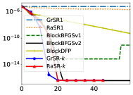
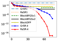
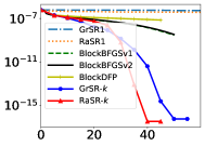
(a) MNIST (iteration)	(b) sido0 (iteration)	(c) gisette (iteration)
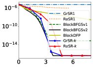
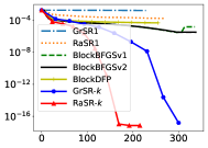
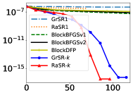
(d) MNIST (time)	(e) sido0 (time)	(f) gisette (time)

Figure 1: We demonstrate “#iteration vs. $\|\nabla f({\bf x})\|$” and “running time (s) vs. $\|\nabla f({\bf x})\|$” on datasets “MNIST”, “sido0” and “gisette”, where we take $k=200$ for all of the block quasi-Newton methods.

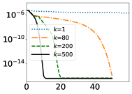
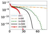
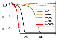
(a) MNIST (iteration)	(b) sido0 (iteration)	(c) gisette (iteration)
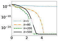
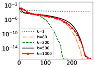
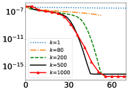
(d) MNIST (time)	(e) sido0 (time)	(f) gisette (time)

Figure 2: We demonstrate “#iteration vs. $\|\nabla f({\bf x})\|$” and “running time (s) vs. $\|\nabla f({\bf x})\|$” on datasets “MNIST”, “sido0” and “Gisette” with different $k=\{1,80,200,500,1000\}$ for RaSR-$k$.

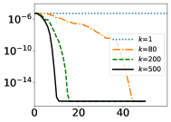
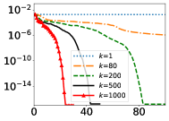
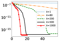
(a) MNIST (iteration)	(b) sido0 (iteration)	(c) gisette (iteration)
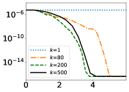
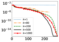
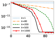
(d) MNIST (time)	(e) sido0 (time)	(f) gisette (time)

Figure 3: We demonstrate “#iteration vs. $\|\nabla f({\bf x})\|$” and “running time (s) vs. $\|\nabla f({\bf x})\|$” on datasets “MNIST”, “Sido0” and “Gisette” with different $k=\{1,80,200,500,1000\}$ for GrSR-$k$.

We conduct the experiments on the model of regularized logistic regression, which can be formulated as

$$\min_{{{\bf x}}\in{\mathbb{R}}^{d}}f({\bf x})\triangleq\frac{1}{n}\sum_{i=1}^{n}\ln\left(1+\exp{-b_{i}{{\bf a}}_{i}^{\top}{\bf x}}\right)+\frac{\gamma}{2}\|{\bf x}\|^{2},$$ (37)

where ${{\bf a}}_{i}\in{\mathbb{R}}^{d}$ and $b_{i}\in\{-1,+1\}$ are the feature and the corresponding label of the $i$-th sample respectively, and $\gamma>0$ is the regularization hyperparameter.

We refer to SR-$k$ methods (Algorithm 1) with randomized and greedy strategies as RaSR-$k$ and GrSR-$k$ respectively. The corresponding SR1 methods with randomized and greedy strategies are referred as RaSR1 and GrSR1 (Algorithm 1 with $k=1$ or Algorithm 4 of Lin et al. [24]) respectively. We also refer to the randomized block BFGS proposed by Gower et al. [15], Gower and Richtárik [14] (Algorithm 2 [15, 14]) as BlockBFGSv1 and refer the new proposed Algorithm 3 with block BFGS and block DFP updates as BlockBFGSv2 and BlockDFP respectively. We compare the proposed RaSR-$k$, GrSR-$k$, BlockBFGSv2 and BlockDFP with baseline methods on problem (37). For all methods, We tune the parameters ${\bf G}_{0}$ and $M$ from $\{{\bf I}_{d},10\cdot{\bf I}_{d},10^{2}\cdot{\bf I}_{d},10^{3}\cdot{\bf I}_{d},10^{4}\cdot{\bf I}_{d}\}$ and $\{1,10,100,1000,10000\}$ respectively. We evaluate the performance for all of methods on three real-world datasets “MNIST”, “sido0” and “gisette”. We conduct our experiments on a PC with Apple M1 and implement all algorithms by Python 3.8.12.

We present the results of “iteration numbers vs. gradient norm” and “running time (second) vs. gradient norm” in Figure 1, which corresponds to the settings of $k=200$ for block quasi-Newton methods RaSR-$k$, GrSR-$k$, BlockBFGSv1, BlockBFGSv2 and BlockDFP. We observe that the proposed SR-$k$ methods (RaSR-$k$ and GrSR-$k$) significantly outperform baselines. Besides, we also observe that BlockBFGS is faster than BlockDFP, which is similar to the advantage of the greedy BFGS method over the greedy DFP method [33].

We also test the performance of SR-$k$ methods under the setting of $k\in\{1,80,200,500,1000\}$. We present the results of RaSR-$k$ and GrSR-$k$ in Figure 2 and 3 respectively. We observe that the larger $k$ leads to faster convergence in terms of the iterations ((a), (b) and (c) of Figure 2 and 3). In addition, we find that SR-$k$ methods with $k>1$ significantly outperform SR-$1$ methods in terms of the running time. This is because the block update can reduce cache miss rate and take the advantage of parallel computing. However, increasing $k$ does not always result less running time because the acceleration caused by the block update is limited by the cache size. Therefore, there is a trade-off between the convergence rate and the running time per iteration in practice. In our experimental environment and candidates of $k$, the RaSR-$k$ method with $k=200$ has the best performance for “MNIST” and “sido0” ((d), (e) of Figure 2) and with $k=500$ has the best performance for “gisette” ((f) of Figure 2); the GrSR-$k$ method with $k=200$ has the best performance for “MNIST” ((d) of Figure 3) and with $k=500$ has the best performance for “sido0” and “gisette” ((e), (f) of Figure 3).

7 Conclusion

In this paper, we have proposed symmetric rank-$k$ (SR-$k$) methods for convex optimization. We have proved SR-$k$ methods enjoy the explicit local superlinear convergence rate of ${\mathcal{O}}\left((1-k/d)^{t(t-1)/2}\right)$. Our result successfully reveals the advantage of block-type updates in quasi-Newton methods, building a bridge between the theories of ordinary quasi-Newton methods and standard Newton method. As a byproduct, we also provide the convergence rate of ${\mathcal{O}}\left((1-k/(\varkappa d))^{t(t-1)/2}\right)$ for randomized block BFGS and randomized block DFP methods.

The application of SR-$k$ methods is not limited to the convex optimization, one can also leverage the idea of SR-$k$ update to solve minimax problems [25, 26]. It is also possible to further accelerate the sharpened quasi-Newton methods [20]. In future work, it would be interesting to establish the global convergence results of SR-$k$ methods by taking the recent advances of Jiang et al. [18] and study the limited memory variant of block quasi-Newton methods by using the displacement aggregation [1].

Appendix A An Elementary Proof of Lemma 3.4(a)

Before prove Lemma 3.4(a), we first provide the following lemma.

Lemma A.1.

Assume ${\bf P}\in{\mathbb{R}}^{d\times k}$ is column orthonormal $(k\leq d)$ and ${\bf{v}}\sim\mathcal{N}_{d}({\bf{0}},{\bf P}{\bf P}^{\top})$ is a $d$-dimensional multivariate normal distributed vector, then we have

$${\mathbb{E}}\left[\frac{{\bf{v}}{\bf{v}}^{\top}}{{\bf{v}}^{\top}{\bf{v}}}\right]=\frac{1}{k}{\bf P}{\bf P}^{\top}.$$

Proof.

The distribution ${\bf{v}}\sim\mathcal{N}_{d}({\bf{0}},{\bf P}{\bf P}^{\top})$ implies there exists a $k$-dimensional normal distributed vector ${{\bf w}}\sim\mathcal{N}_{k}({\bf{0}},{\bf I}_{k})$ such that ${\bf{v}}={\bf P}{{\bf w}}$. Thus, we have

$${\mathbb{E}}\left[\frac{{\bf{v}}{\bf{v}}^{\top}}{{\bf{v}}^{\top}{\bf{v}}}\right]= {\mathbb{E}}\left[\frac{({\bf P}{{\bf w}})({\bf P}{{\bf w}})^{\top}}{({\bf P}{{\bf w}})^{\top}({\bf P}{{\bf w}})}\right]={\mathbb{E}}\left[\frac{{\bf P}{{\bf w}}{{\bf w}}^{\top}{\bf P}^{\top}}{{{\bf w}}^{\top}{\bf P}^{\top}{\bf P}{{\bf w}}}\right]$$

$$= {\bf P}{\mathbb{E}}\left[\frac{{{\bf w}}{{\bf w}}^{\top}}{{{\bf w}}^{\top}{{\bf w}}}\right]{\bf P}^{\top}=\frac{1}{k}{\bf P}{\bf P}^{\top},$$

where the last step is because of ${{\bf w}}/\left\|{{\bf w}}\right\|_{2}$ is uniform distributed on $k$-dimensional unit sphere and its covariance matrix is $k^{-1}{\bf I}_{k}$.

∎

Now we prove statement (a) of Lemma 3.4.

Proof.

We prove this result by induction on $k$. We only need to prove equation (16).

The induction base $k=1$ have been verified by Lemma A.1. Now we assume

$${\mathbb{E}}\left[{\bf U}({\bf U}^{\top}{\bf U})^{-1}{\bf U}^{\top}\right]=\frac{k}{d}{\bf I}_{d}$$

holds for any ${\bf U}\in{\mathbb{R}}^{d\times k}$ that each of its entries are independently distributed according to ${\mathcal{N}}(0,1)$. We define the random matrix

$$\hat{{\bf U}}=\begin{bmatrix}{\bf U}&{\bf{v}}\end{bmatrix}\in{\mathbb{R}}^{d\times(k+1)},$$

where ${\bf{v}}\sim{\mathcal{N}}_{d}({\bf{0}},{\bf I}_{d})$ is independent distributed to ${\bf U}$. We define ${\bf B}={\bf U}({\bf U}^{\top}{\bf U})^{-1}{\bf U}^{\top}$, then we use block matrix inversion formula to compute $(\hat{{\bf U}}^{\top}\hat{{\bf U}})^{-1}$:

$$(\hat{{\bf U}}^{\top}\hat{{\bf U}})^{-1}$$

$$=\left(\begin{bmatrix}{\bf U}^{\top}\\ {\bf{v}}^{\top}\end{bmatrix}\begin{bmatrix}{\bf U}&{\bf{v}}\end{bmatrix}\right)^{-1}=\left(\begin{bmatrix}{\bf U}^{\top}{\bf U}&{\bf U}^{\top}{\bf v}\\ {\bf v}^{\top}{\bf U}&{\bf v}^{\top}{\bf v}\end{bmatrix}\right)^{-1}$$

$$=\begin{bmatrix}({\bf U}^{\top}{\bf U})^{-1}+({\bf U}^{\top}{\bf U})^{-1}{\bf U}^{\top}{\bf v}({\bf v}^{\top}({\bf I}-{\bf B}){\bf v})^{-1}{\bf v}^{\top}{\bf U}({\bf U}^{\top}{\bf U})^{-1}&~{}-({\bf U}^{\top}{\bf U})^{-1}{\bf U}^{\top}{\bf v}({\bf v}^{\top}({\bf I}-{\bf B}){\bf v})^{-1}\\ -({\bf v}^{\top}({\bf I}-{\bf B}){\bf v})^{-1}{\bf v}^{\top}{\bf U}({\bf U}^{\top}{\bf U})^{-1}&~{}({\bf v}^{\top}({\bf I}-{\bf B}){\bf v})^{-1}\end{bmatrix}.$$

Thus, we have

$$\hat{{\bf U}}(\hat{{\bf U}}^{\top}\hat{{\bf U}})^{-1}\hat{{\bf U}}^{\top}$$

$$=\begin{bmatrix}{\bf U}&{\bf{v}}\end{bmatrix}\left(\begin{bmatrix}{\bf U}^{\top}\\ {\bf{v}}^{\top}\end{bmatrix}\begin{bmatrix}{\bf U}&{\bf{v}}\end{bmatrix}\right)^{-1}\begin{bmatrix}{\bf U}^{\top}\\ {\bf{v}}^{\top}\end{bmatrix}$$

$$={\bf B}+\frac{{\bf B}{\bf v}{\bf v}^{\top}{\bf B}}{{\bf v}^{\top}({\bf I}-{\bf B}){\bf v}}-\frac{{\bf B}{\bf v}{\bf v}^{\top}}{{\bf v}^{\top}({\bf I}-{\bf B}){\bf v}}-\frac{{\bf v}{\bf v}^{\top}{\bf B}}{{\bf v}^{\top}({\bf I}-{\bf B}){\bf v}}+\frac{{\bf v}{\bf v}^{\top}}{{\bf v}^{\top}({\bf I}-{\bf B}){\bf v}}$$

$$={\bf B}+\frac{({\bf I}_{d}-{\bf B}){\bf{v}}{\bf{v}}^{\top}({\bf I}_{d}-{\bf B})}{{\bf{v}}^{\top}({\bf I}_{d}-{\bf B}){\bf{v}}}.$$

Since the rank of projection matrix ${\bf I}_{d}-{\bf B}$ is $d-k$, we can write ${\bf I}_{d}-{\bf B}={\bf Q}{\bf Q}^{\top}$ for some column orthonormal matrix ${\bf Q}\in{\mathbb{R}}^{d\times(d-k)}$. Thus, we achieve

$${\mathbb{E}}[\hat{{\bf U}}(\hat{{\bf U}}^{\top}\hat{{\bf U}})\hat{{\bf U}}^{\top}]$$

$$= \frac{k}{d}{\bf I}_{d}+{\mathbb{E}}_{{\bf U}}\left[{\mathbb{E}}_{{\bf{v}}}\left[\frac{({\bf I}_{d}-{\bf B}){\bf{v}}{\bf{v}}^{\top}({\bf I}_{d}-{\bf B})}{{\bf{v}}^{\top}({\bf I}_{d}-{\bf B}){\bf{v}}}\,\Bigg{|}\,{\bf U}\right]\right]$$

$$= \frac{k}{d}{\bf I}_{d}+{\mathbb{E}}_{{\bf U}}\left[{\mathbb{E}}_{{\bf{v}}}\left[\frac{({\bf Q}{\bf Q}^{\top}{\bf{v}})({\bf{v}}^{\top}{\bf Q}{\bf Q}^{\top})}{({\bf{v}}^{\top}{\bf Q}{\bf Q}^{\top})({\bf Q}{\bf Q}^{\top}{\bf{v}})}\,\Bigg{|}\,{\bf U}\right]\right]$$

$$= \frac{k}{d}{\bf I}_{d}+\frac{1}{d-k}{\mathbb{E}}_{{\bf U}}[{\bf Q}{\bf Q}^{\top}]$$

$$= \frac{k}{d}{\bf I}_{d}+\frac{1}{d-k}{\mathbb{E}}_{{\bf U}}[{\bf I}_{d}-{\bf B}]$$

$$= \frac{k}{d}{\bf I}_{d}+\frac{1}{d-k}\left({\bf I}_{d}-\frac{k}{d}{\bf I}_{d}\right)$$

$$= \frac{k+1}{d}{\bf I}_{d},$$

which completes the induction. In above derivation, the second equality is due to Lemma A.1 and the fact ${\bf Q}{\bf Q}^{\top}{\bf{v}}\sim\mathcal{N}_{d}({\bf{0}},{\bf Q}{\bf Q}^{\top})$; the third equality comes from the inductive hypothesis.

∎

Appendix B Auxiliary Lemmas for Non-negative Sequences

We provide the following lemmas on non-negative sequences, which will be useful to obtain the explicit convergence rates of the proposed block quasi-Newton methods.

Lemma B.1.

Let $\{\lambda_{t}\}$ and $\{\delta_{t}\}$ be two non-negative random sequences that satisfy

$$\begin{split}&\lambda_{t+1}\leq(1+c_{1}\lambda_{t})^{2}(\delta_{t}+c_{2}\lambda_{t})\lambda_{t},~{}~{}~{}{\mathbb{E}}_{t}\left[\delta_{t+1}\right]\leq\left(1-\frac{1}{\alpha}\right)(1+m\lambda_{t})^{2}(\delta_{t}+c_{3}\lambda_{t}),\\ &\delta_{0}+c\lambda_{0}\leq s,~{}~{}~{}\text{and}~{}~{}~{}\lambda_{t}\leq\left(1-\frac{1}{\beta}\right)^{t}\lambda_{0},\end{split}$$ (38)

for some $c_{1},c_{2},c_{3}\geq 0$ with $c=\max\{c_{2},c_{3}\}$, $s\geq 0$, $\alpha>1$, and $\beta\in(0,1)$, where ${\mathbb{E}}_{t}[\,\cdot\,]\triangleq{\mathbb{E}}[\,\cdot\,|\delta_{0},\cdots,\delta_{t},\lambda_{0},\cdots,\lambda_{t}]$. If $\lambda_{0}$ is sufficient small such that

$$\lambda_{0}\leq\frac{\ln 2}{\beta(2c_{1}+c(\alpha/(\alpha-1)))}$$ (39)

then it holds that

$${\mathbb{E}}\left[\frac{\lambda_{t+1}}{\lambda_{t}}\right]\leq 2\left(1-\frac{1}{\alpha}\right)^{t}s.$$

Proof.

We denote

$$\theta_{t}\triangleq\delta_{t}+c\lambda_{t}.$$ (40)

Since the index $t+1\geq 1$, we have

$${\mathbb{E}}_{t}[\delta_{t+1}]\overset{\eqref{eq:supercondi}}{\leq}\left(1-\frac{1}{\alpha}\right)(1+c_{1}\lambda_{t})^{2}(\delta_{t}+c\lambda_{t})\leq\left(1-\frac{1}{\alpha}\right)\theta_{t}\exp{2c_{1}\lambda_{t}}\quad\text{and}\quad\lambda_{t+1}\overset{\eqref{eq:supercondi}}{\leq}\theta_{t}\lambda_{t}\exp{2c_{1}\lambda_{t}}.$$ (41)

We denote $\tilde{c}\triangleq 2c_{1}+c\alpha/(\alpha-1)$, then it holds that

$$\begin{split}{\mathbb{E}}_{t}[\theta_{t+1}]&\overset{\eqref{eq:thetadef}}{\leq}\left(1-\frac{1}{\alpha}\right)\cdot\left(1+\frac{\alpha c\lambda_{t}}{\alpha-1}\right)\theta_{t}\exp{2c_{1}\lambda_{t}}\leq\left(1-\frac{1}{\alpha}\right)\theta_{t}\exp{(2c_{1}+c\alpha/(\alpha-1))\lambda_{t}}\\ &=\left(1-\frac{1}{\alpha}\right)\theta_{t}\exp{\tilde{c}\lambda_{t}}\overset{\eqref{eq:supercondi}}{\leq}\left(1-\frac{1}{\alpha}\right)\theta_{t}\exp{\tilde{c}(1-{1}/{\beta})^{t}\lambda_{0}}.\end{split}$$ (42)

Taking expectation on both sides of (42), we have

$${\mathbb{E}}[\theta_{t+1}]\leq\left(1-\frac{1}{\alpha}\right)\exp{{\tilde{c}}(1-{1}/{\beta})^{t}\lambda_{0}}{\mathbb{E}}[\theta_{t}],$$ (43)

where we use the fact ${\mathbb{E}}[{\mathbb{E}}_{t}[\delta_{t+1}]]={\mathbb{E}}[\delta_{t+1}]$. Therefore, we have

$${\mathbb{E}}\left[\frac{\lambda_{t+1}}{\lambda_{t}}\right] \overset{\eqref{eq:lambdat_leq_thetat}}{\leq}{\mathbb{E}}[\theta_{t}\exp{2c_{1}\lambda_{t}}]{\leq}\left(1-\frac{1}{\alpha}\right){\mathbb{E}}\left[\theta_{t}\right]\exp{\tilde{c}(1-{1}/{\beta})^{t}\lambda_{0}}$$

$$\overset{\eqref{eq:expthetat}}{\leq}\left(1-\frac{1}{\alpha}\right)^{2}{\mathbb{E}}\left[\theta_{t-1}\right]\exp{(\tilde{c}(1-{1}/{\beta})^{t}+\tilde{c}(1-{1}/{\beta})^{t-1})\lambda_{0}}$$

$$\overset{\eqref{eq:expthetat}}{\leq}\left(1-\frac{1}{\alpha}\right)^{t}{\mathbb{E}}\left[\theta_{0}\right]\exp{\tilde{c}\sum_{p=0}^{t}(1-{1}/{\beta})^{p}\lambda_{0}}$$

$$~{}~{}{\leq}~{}~{}\left(1-\frac{1}{\alpha}\right)^{t}{\mathbb{E}}\left[\theta_{0}\right]\exp{\tilde{c}\beta\lambda_{0}}\overset{\eqref{eq:supercondiini},\eqref{eq:supercondi}}{\leq}\left(1-\frac{1}{\alpha}\right)^{t}2s.$$

∎

Lemma B.2.

Let $\{\lambda_{t}\}$ and $\{\tilde{\eta}_{t}\}$ be two positive sequences where $\tilde{\eta}_{t}\geq 1$ that satisfy

$$\begin{split}&\lambda_{t+1}\leq\left(1-\frac{1}{\tilde{\eta}_{t}}\right)\lambda_{t}+\frac{m_{1}\lambda_{t}^{2}}{2}+\frac{m_{1}^{2}\lambda_{t}^{3}}{4\tilde{\eta}_{t}}~{}~{}~{}\text{for}~{}~{}~{}{m_{1}\lambda_{t}\leq 2},\\ &\tilde{\eta}_{t+1}\leq(1+m_{2}\lambda_{t})^{2}\tilde{\eta}_{t},\end{split}$$ (44)

for some $m_{1}$ and $m_{2}>0$. If

$$m\lambda_{0}\leq\frac{\ln({3}/{2})}{4\tilde{\eta}_{0}},$$ (45)

where $m\triangleq\max\{m_{1},m_{2}\}$, then it holds that

$$\tilde{\eta}_{t}\leq\tilde{\eta}_{0}\exp{2m\sum_{i=0}^{t-1}\lambda_{t}}\leq\frac{3\tilde{\eta}_{0}}{2}$$ (46)

and

$$\lambda_{t} \leq\left(1-\frac{1}{2\tilde{\eta}_{0}}\right)^{t}\lambda_{0}.$$ (47)

Proof.

Our analysis follows the proof Theorem 4.7 of Rodomanov and Nesterov [33] and Theorem 23 of Lin et al. [24]. We prove results of (46) and (47) by induction. In the case of $t=0$, inequalities (46) and (47) are satisfied naturally. Now we suppose inequalities (46) and (47) holds for $t=0,\dots,\hat{t}$, then we have

$$m\sum_{i=0}^{\hat{t}}\lambda_{i}\overset{\eqref{eq:lambda_t_linear}}{\leq}m\lambda_{0}\sum_{i=0}^{\hat{t}}\left(1-\frac{1}{2\tilde{\eta}_{0}}\right)^{i}\leq 2\tilde{\eta}_{0}m\lambda_{0}\overset{\eqref{eq:linear_initial}}{\leq}1.$$ (48)

In the case of $t=\hat{t}+1$ we have

$$\frac{1-{m_{1}\lambda_{\hat{t}}}/{2}}{\tilde{\eta}_{\hat{t}}}{\geq}\frac{\exp{-m_{1}\lambda_{\hat{t}}}}{\tilde{\eta}_{\hat{t}}}\overset{\eqref{eq:tilde_eta}}{\geq}\frac{\exp{-2m\sum_{i=0}^{t}\lambda_{i}}}{\tilde{\eta}_{0}}\geq\frac{2}{3\tilde{\eta}_{0}}\qquad\text{and}\qquad m\lambda_{\hat{t}}\leq m\lambda_{0}\overset{\eqref{eq:linear_initial}}{\leq}\frac{1}{8\tilde{\eta}_{0}}.$$ (49)

According to condition (44), we have

$$\lambda_{\hat{t}+1} \overset{\eqref{eq:lambda_t_1}}{\leq}\left(1+\frac{m_{1}\lambda_{\hat{t}}}{2}\right)\cdot\left(1-\frac{1-{m_{1}\lambda_{\hat{t}}}/{2}}{\tilde{\eta}_{\hat{t}}}\right)\lambda_{\hat{t}}\overset{\eqref{eq:simple_induct}}{\leq}\left(1-\frac{1}{2\tilde{\eta}_{0}}\right)\lambda_{\hat{t}}\leq\left(1-\frac{1}{2\tilde{\eta}_{0}}\right)^{{\hat{t}}+1}\lambda_{0},$$

where the last step is based on induction. We also have

$$\tilde{\eta}_{\hat{t}+1}\overset{\eqref{eq:thetat+1leqs}}{\leq}(1+m_{2}\lambda_{\hat{t}})^{2}\tilde{\eta}_{t}\leq\tilde{\eta}_{\hat{t}}\exp{2m\lambda_{\hat{t}}}\overset{\eqref{eq:tilde_eta}}{\leq}\tilde{\eta}_{0}\exp{2m\sum_{i=0}^{\hat{t}}\lambda_{\hat{t}}}\overset{\eqref{eq:linear_initial}}{\leq}\frac{3\tilde{\eta}_{0}}{2}.$$

∎

Appendix C The Proof Details of Theorem 4.2

We first provide a lemma from Lin et al. [24].

Lemma C.1 ([24, Lemma 25]).

If the twice differentiable function $f:{\mathbb{R}}^{d}\to{\mathbb{R}}$ is $M$-strongly self-concordant and $\mu$-strongly convex and the positive definite matrix ${\bf G}\in{\mathbb{R}}^{d\times d}$ and ${{\bf x}}\in{\mathbb{R}}^{d}$ satisfy $\nabla^{2}f({\bf x})\preceq{\bf G}\preceq\eta\nabla^{2}f({\bf x})$ for some $\eta>1$, then we have

$$\nabla^{2}f({\bf x}_{+})\preceq\tilde{{\bf G}}\preceq\eta(1+Mr)^{2}\nabla^{2}f({\bf x}_{+}),$$ (50)

and

$$\tau_{\nabla^{2}f({\bf x}_{+})}(\tilde{{\bf G}})\leq(1+Mr)^{2}\left(\frac{\tau_{\nabla^{2}f({\bf x})}({\bf G})}{{\rm tr}\left(\nabla^{2}f({\bf x})\right)}+2Mr\right){\rm tr}\left(\nabla^{2}f({\bf x}_{+})\right)$$ (51)

for any ${{\bf x}}_{+}\in{\mathbb{R}}^{d}$, where $\tilde{{\bf G}}=(1+Mr){\bf G}$, $r=\|{\bf x}-{\bf x}_{+}\|_{{\bf x}}$ and the notations of $\tau_{\bf H}({\bf G})$ follow the expressions of (10).

Now, we provide the detailed proof of Theorem 4.2 by incorporating Lemma 4.1, C.1, B.2 and the property for the SR-$k$ update of Lemma 3.2.

Proof.

We denote $\lambda_{t}\triangleq\lambda({\bf x}_{t})$ and $\tilde{\eta}_{t}\triangleq\min_{\nabla^{2}f({\bf x}_{t})\preceq\eta{\bf G}_{t}}\eta$, which means

$$\nabla^{2}f({\bf x}_{t})\preceq{\bf G}_{t}\preceq\tilde{\eta}_{t}\nabla^{2}f({\bf x}_{t}).$$

According to Lemma 4.1, we have

$$\lambda_{t+1}\leq\left(1-\frac{1}{\tilde{\eta}_{t}}\right)\lambda_{t}+\frac{M\lambda_{t}^{2}}{2}+\frac{M^{2}\lambda_{t}^{3}}{4\tilde{\eta}_{t}}.$$

Using Lemma C.1, it holds that

$$\nabla^{2}f({\bf x}_{t+1})\preceq\tilde{{\bf G}}_{t}\preceq(1+Mr_{t})^{2}\tilde{\eta}_{t}\nabla^{2}f({\bf x}_{t}).$$

By Lemma 3.2, it is satisfied that

$$\nabla^{2}f({\bf x}_{t+1})\overset{\eqref{eq:srk_good}}{\preceq}{\bf G}_{t+1}\overset{\eqref{eq:srk_good}}{\preceq}(1+Mr_{t})^{2}\tilde{\eta}_{t}\nabla^{2}f({\bf x}_{t+1})\overset{\eqref{eq:linear-quadra}}{\preceq}(1+M\lambda_{t})^{2}\tilde{\eta}_{t}\nabla^{2}f({\bf x}_{t+1}),$$

which means

$$\tilde{\eta}_{t+1}\leq(1+M\lambda_{t})^{2}\tilde{\eta}_{t}.$$

Hence, the sequences $\{\tilde{\eta}_{t}\}$ and $\{\lambda_{t}\}$ satisfy the conditions of Lemma B.2 with $m_{1}=m_{2}=M$, then we obtain

$$\nabla^{2}f({\bf x}_{t})\preceq\tilde{{\bf G}}_{t}\preceq\frac{3\tilde{\eta}_{0}}{2}\nabla^{2}f({\bf x}_{t})\preceq\frac{3{\eta}_{0}}{2}\nabla^{2}f({\bf x}_{t}),$$

and

$$\lambda({\bf x}_{t})\leq\left(1-\frac{1}{2\tilde{\eta}_{0}}\right)^{t}\lambda({\bf x}_{0})\leq\left(1-\frac{1}{2{\eta}_{0}}\right)^{t}\lambda({\bf x}_{0}).$$

∎

∎

Appendix D The Proof Details of Theorem 4.3

We first provide some auxiliary lemmas which will be used in our later proof.

Lemma D.1.

For any positive definite symmetric matrices ${\bf G},{\bf H}\in{\mathbb{R}}^{d\times d}$ such that ${\bf H}\preceq{\bf G}$, it holds that

$${\bf G}\preceq\left(1+\frac{\hat{\varkappa}d\tau_{{\bf H}}({\bf G})}{{\rm tr}\left({\bf H}\right)}\right){\bf H}.$$ (52)

If it further holds that ${\bf G}\preceq\eta{\bf H}$, then we have

$$\qquad\frac{\tau_{{\bf H}}({\bf G})}{{\rm tr}\left({\bf H}\right)}\leq\eta-1,$$ (53)

where $\hat{\varkappa}$ is the condition number of ${\bf H}$ and the notation of $\tau_{\bf H}({\bf G})$ follow the expression of (10).

Proof.

The inequality (52) is directly obtained by following statement 3) of Equation (42) by Lin et al. [24, Lemma 25]. The inequality (53) is obtained by the definition of $\tau_{{\bf H}}({\bf G})$, that is

$$\frac{\tau_{{\bf H}}({\bf G})}{{\rm tr}\left({\bf H}\right)}=\frac{{\rm tr}\left(({\bf G}-{\bf H})\right)}{{\rm tr}\left({\bf H}\right)}{\leq}\frac{{\rm tr}\left((\eta-1){\bf H}\right)}{{\rm tr}\left({\bf H}\right)}=\eta-1.$$

∎∎

Lemma D.2 ([24, Lemma 26]).

Suppose the non-negative random sequences $\{X_{t}\}$ satisfies ${\mathbb{E}}[X_{t}]\leq a\left(1-{1}/{\alpha}\right)^{t}$ for all $t\geq 0$ and some constants $a\geq 0$ and $\alpha>1$. Then for any $\delta\in(0,1)$, we have

$$X_{t}\leq\frac{a\alpha^{2}}{\delta}\cdot\left(1-\frac{1}{1+\alpha}\right)^{t}$$

for all $t$ with probability at least $1-\delta$.

Now, we provide the proof of Theorem 4.3

Proof.

Denote $g_{t}={{\rm tr}\left({\bf G}_{t}-\nabla^{2}f({\bf x}_{t})\right)}/{{\rm tr}\left(\nabla^{2}f({\bf x}_{t})\right)}$, $\delta_{t}=d\varkappa g_{t}$, $\lambda_{t}=\lambda({\bf x}_{t})$ and ${\mathbb{E}}_{t}[\,\cdot\,]\triangleq{\mathbb{E}}[\,\cdot\,|\,{\bf U}_{0},\cdots,{\bf U}_{t-1}]$. From Theorem 3.6, we have

$${\mathbb{E}}_{t}\left[{\rm tr}\left({\bf G}_{t+1}-\nabla^{2}f({\bf x}_{t+1})\right)\right]\leq\left(1-\frac{k}{d}\right){\rm tr}\left(\tilde{{\bf G}}_{t}-\nabla^{2}f({\bf x}_{t+1})\right),$$ (54)

From Lemma C.1, we have

$${\mathbb{E}}_{t}[\tau_{\nabla^{2}f({\bf x}_{t+1})}(\tilde{{\bf G}}_{t})]\overset{\eqref{eq:delta_SRK_lin}}{\leq}(1+Mr_{t})^{2}(g_{t}+2Mr_{t}){\rm tr}\left(\nabla^{2}f({\bf x}_{t+1})\right),$$

which means

$${\mathbb{E}}_{t}[\delta_{t+1}]\overset{\eqref{eq:linear-quadra},\,\eqref{eq:srk_G-H}}{\leq}\left(1-\frac{k}{d}\right)(1+M\lambda_{t})^{2}(\delta_{t}+2\varkappa dM\lambda_{t}).$$ (55)

The initial condition (24) means the results of Theorem 4.2 hold, that is

$$\lambda_{t}\leq\left(1-\frac{1}{2\eta_{0}}\right)^{t}\lambda_{0}\qquad\text{and}\qquad\nabla^{2}f({\bf x}_{t})\preceq{\bf G}_{t}.$$ (56)

According to Lemma D.1 and the definition of $\delta_{t}$, we have

$$\nabla^{2}f({\bf x}_{t})\overset{\eqref{eq:linearrate}}{\preceq}{\bf G}_{t}\overset{\eqref{eq:GHneq}}{\preceq}(1+\delta_{t})\nabla^{2}f({\bf x}_{t}).$$

According to Lemma 4.1, we have

$$\lambda_{t+1} \overset{\eqref{eq:linear-quadra}}{\leq}\left(1-\frac{1}{1+\delta_{t}}\right)\lambda_{t}+\frac{M\lambda_{t}^{2}}{\eta_{t}}+\frac{M^{2}\lambda_{t}^{3}}{4\eta_{t}}$$

$$\,\,\leq\left(1+\frac{M\lambda_{t}}{2}\right)\cdot\left(\frac{\delta_{t}+{M\lambda_{t}}/{2}}{1+\delta_{t}}\right)\lambda_{t}$$

$$\,\,\leq\left(1+M\lambda_{t}\right)^{2}\left(\delta_{t}+\frac{M}{2}\lambda_{t}\right)\lambda_{t}.$$

According to Lemma D.1 and the initial condition (24), we have

$$\delta_{0}=d\varkappa g_{0}\overset{\eqref{eq:GHneq_2}}{\leq}(\eta_{0}-1)d\varkappa~{}~{}~{}\text{and}~{}~{}~{}\theta_{0}=\delta_{0}+2d\varkappa M\lambda_{0}\overset{\eqref{eq:initial}}{\leq}\eta_{0}d\varkappa.$$ (57)

Hence, the random sequences of $\{\lambda_{t}\}$ and $\{\delta_{t}\}$ satisfies the conditions of Lemma B.1 with

$$c_{1}=M,\quad c_{2}=\frac{M}{2},\quad c_{3}=2\varkappa dM,\quad\alpha=\frac{d}{k},\quad\beta=\frac{1}{2\eta_{0}},\quad\text{and}\quad s=\eta_{0}d\varkappa,$$

which means we can obtain inequality (25).

Now, we prove the two-stage convergence of SR-$k$ methods.

1. For SR-$k$ method with randomized strategy $\left[{\bf U}_{t}\right]_{ij}\overset{\rm{i.i.d}}{\sim}{{\mathcal{N}}(0,1)}$, we apply Lemma D.2 with $\alpha=d/k$ and $a=2d\varkappa\eta_{0}$ to obtain

   $$\frac{\lambda_{t+1}}{\lambda_{t}}\leq\frac{2d^{2}\varkappa\eta_{0}}{k\delta}\cdot\left(1-\frac{k}{d+k}\right)^{t}$$ (58)

   holds for all $t$ with probability at least $1-\delta$. Take $t_{0}={\mathcal{O}}(d\ln(\eta_{0}\varkappa d)/k)$, which satisfies that

   $$\frac{2d^{2}\varkappa\eta_{0}}{k\delta}\cdot\left(1-\frac{k}{d+k}\right)^{t_{0}}\leq\frac{1}{2},$$ (59)

   together with the linear rate (23), we have

   $$\begin{split}\lambda_{t+t_{0}}&\overset{\eqref{eq:rasrk_super}}{\leq}\left(1-\frac{k}{d+k}\right)^{t+t_{0}}2d\varkappa\eta_{0}d\lambda_{t+t_{0}-1}\\ &\overset{\eqref{eq:rasrk_t0}}{\leq}\left(1-\frac{k}{d+k}\right)^{t}\cdot\frac{\lambda_{t+t_{0}-1}}{2}\leq\cdots\overset{\eqref{eq:rasrk_super},\eqref{eq:rasrk_t0}}{\leq}\left(1-\frac{k}{d+k}\right)^{t(t-1)/2}\cdot\left(\frac{1}{2}\right)^{t}\lambda_{t_{0}}\\ &\overset{\eqref{eq:srklinear}}{\leq}\left(1-\frac{k}{d+k}\right)^{t(t-1)/2}\cdot\left(\frac{1}{2}\right)^{t}\cdot\left(1-\frac{1}{2\eta_{0}}\right)^{t_{0}}\lambda_{0}.\end{split}$$

   with probability at least $1-\delta$.

2. For SR-$k$ method with greedy strategy ${\bf U}_{t}={\bf E}_{k}(\tilde{{\bf G}}_{t}-\nabla^{2}f({\bf x}_{t+1}))$, we choose $t_{0}={\mathcal{O}}\left(d\ln(\eta_{0}\varkappa d)/k\right)$ such that

   $$\left(1-\frac{k}{d}\right)^{t_{0}}2d\varkappa\eta_{0}\leq\frac{1}{2},$$ (60)

   together with the linear rate (23), we have

   $$\begin{split}\lambda_{t+t_{0}}&\overset{\eqref{eq:E_lambda_srk}}{\leq}\left(1-\frac{k}{d}\right)^{t+t_{0}}2d\varkappa\eta_{0}d\lambda_{t+t_{0}-1}\\ &\overset{\eqref{eq:grsrk_t0}}{\leq}\left(1-\frac{k}{d}\right)^{t}\cdot\frac{\lambda_{t+t_{0}-1}}{2}\leq\cdots\overset{\eqref{eq:E_lambda_srk},\eqref{eq:grsrk_t0}}{\leq}\left(1-\frac{k}{d}\right)^{t(t-1)/2}\cdot\left(\frac{1}{2}\right)^{t}\lambda_{t_{0}}\\ &\overset{\eqref{eq:srklinear}}{\leq}\left(1-\frac{k}{d}\right)^{t(t-1)/2}\cdot\left(\frac{1}{2}\right)^{t}\cdot\left(1-\frac{1}{2\eta_{0}}\right)^{t_{0}}\lambda_{0}.\end{split}$$

∎∎

Appendix E The Proof Details of Theorem 5.5

We first provide a lemma which shows the linear convergence for the proposed block BFGS and DFP method (Algorithm 3).

Lemma E.1.

Under the setting of Theorem 5.5, Algorithm 3 holds that

$$\lambda({{\bf x}}_{t})\leq\left(1-\frac{1}{2\eta_{0}}\right)^{t}\lambda({{\bf x}}_{0})~{}~{}~{}\text{and}~{}~{}~{}\nabla^{2}f({\bf x}_{t})\preceq{\bf G}_{t}\preceq\frac{3\eta_{0}}{2}\nabla^{2}f({\bf x}_{t})$$ (61)

for all $t\geq 0$.

Proof.

We can obtain this result by following the proof of Theorem 4.2 by replacing the steps of using Lemma 3.2 with using Lemma 5.2. ∎

We then provide some auxiliary lemmas from Rodomanov and Nesterov [33], Lin et al. [24].

Lemma E.2 ([33, Lemma 4.8.]).

If the twice differentiable function $f:{\mathbb{R}}^{d}\to{\mathbb{R}}$ is $M$-strongly self-concordant and $\mu$-strongly convex and the positive definite matrix ${\bf G}\in{\mathbb{R}}^{d\times d}$ and ${{\bf x}}\in{\mathbb{R}}^{d}$ satisfy $\nabla^{2}f({\bf x})\preceq{\bf G}\preceq\eta\nabla^{2}f({\bf x})$ for some $\eta>1$, then we have

$$\sigma_{\nabla^{2}f({\bf x}_{+})}(\tilde{{\bf G}})\leq(1+Mr)^{2}(\sigma_{\nabla^{2}f({\bf x})}({{\bf G}})+2dMr),$$ (62)

for any ${{\bf x}},{{\bf x}}_{+}\in{\mathbb{R}}^{d}$ where $\tilde{{\bf G}}=(1+Mr){\bf G}$, $r=\|{\bf x}-{\bf x}_{+}\|_{{\bf x}}$ and $\sigma_{\bf H}({\bf G})$ follow the expression of (29).

Lemma E.3.

For any positive definite symmetric matrices ${\bf G},{\bf H}\in{\mathbb{R}}^{d\times d}$ such that ${\bf H}\preceq{\bf G}$, it holds that

$${\bf G}\preceq(1+\sigma_{{\bf H}}({\bf G})){\bf H}.$$ (63)

If it further holds that ${\bf G}\preceq\eta{\bf H}$, then we have

$$\sigma_{{\bf H}}({\bf G})\leq d(\eta-1)$$ (64)

where $\hat{\varkappa}$ is the condition number of ${\bf H}$ and the notation of $\sigma_{\bf H}({\bf G})$ follow the expression of (29).

Proof.

The inequality (63) is directly obtained by following the statement 1) of Equation (42) by Lin et al. [24, Lemma 25]. The inequality (64) is obtained by the definition of $\sigma_{{\bf H}}({\bf G})$, that is

$$\sigma_{{\bf H}}({\bf G})={\rm tr}\left({\bf H}^{-1}({\bf G}-{\bf H})\right)={\rm tr}\left({\bf H}^{-1/2}({\bf G}-{\bf H}){\bf H}^{-1/2}\right)\leq{\rm tr}\left((\eta-1){\bf H}^{-1/2}{\bf H}{\bf H}^{-1/2}\right)=(\eta-1)d.$$

∎

Now we are ready to present the proof for Theorem 5.5.

Proof.

We denote $\delta_{t}\triangleq{\rm tr}\left(({\bf G}_{t}-\nabla^{2}f({\bf x}_{t}))(\nabla^{2}f({\bf x}_{t}))^{-1}\right)$ and $\lambda_{t}\triangleq\lambda({\bf x}_{t})$. The initial condition means we have the results of Lemma E.1. According to Lemma D.1, we have

$$\nabla^{2}f({\bf x}_{t})\overset{\eqref{eq:BFGSlinear}}{\preceq}{\bf G}_{t}\preceq(1+\delta_{t})\nabla^{2}f({\bf x}_{t}).$$

Using Theorem 5.3, we have

$${\mathbb{E}}_{t}[\delta_{t+1}]={\mathbb{E}}_{t}[\sigma_{\nabla^{2}f({\bf x}_{t+1})}({\bf G}_{t+1})]\overset{\eqref{eq:bfgssigma}}{\leq}\left(1-\frac{k}{d\varkappa}\right)\sigma_{\nabla^{2}f({\bf x}_{k+1})}(\tilde{{\bf G}}_{t}).$$ (65)

Using Lemma E.2, we have

$$\sigma_{\nabla^{2}f({\bf x}_{k+1})}(\tilde{{\bf G}}_{t})\overset{\eqref{eq:delta_BFGS_lin}}{\leq}(1+Mr_{t})^{2}(\delta_{t}+2dMr_{t}).$$ (66)

Thus, we can obtain following result

$${\mathbb{E}}_{t}[\delta_{t+1}]\overset{\eqref{eq:linear-quadra}\,\eqref{eq:BFGSconverge1}\,\eqref{eq:BFGSconverge2}}{\leq}\left(1-\frac{k}{d\varkappa}\right)(1+M\lambda_{t})^{2}(\delta_{t}+2dM\lambda_{t}).$$

According to Lemma 4.1, we have

$$\lambda_{t+1}\overset{\eqref{eq:linear-quadra}}{\leq}\left(1+\frac{M\lambda_{t}}{2}\right)\cdot\frac{\delta_{t}+{M\lambda_{t}}/{2}}{1+\delta_{t}}\lambda_{t}\leq(1+M\lambda_{t})^{2}(\delta_{t}+2dM\lambda_{t})\lambda_{t}.$$

According to Lemma E.1, we have

$$\lambda_{t}\leq\left(1-\frac{1}{2\eta_{0}}\right)^{t}\lambda_{0}.$$

According to Lemma E.3 and the initial condition (36), we have

$$\delta_{0}={\rm tr}\left(({\bf G}_{0}-\nabla^{2}f({\bf x}_{0}))(\nabla^{2}f({\bf x}_{0}))^{-1}\right)\overset{\eqref{eq:GHneq_2_bfgs}}{\leq}d(\eta_{0}-1)~{}~{}~{}\text{and}~{}~{}~{}\theta_{0}=\delta_{0}+2dM\lambda_{0}\overset{\eqref{eq:bfgsini}}{\leq}d\eta_{0}.$$

Hence, the random sequences of $\{\lambda_{t}\}$ and $\{\delta_{t}\}$ satisfy the conditions of Lemma B.1 with

$$c_{1}=M,\quad c_{2}=2dM,\quad c_{3}=2dM,\quad\alpha=\frac{d\varkappa}{k},\quad\beta={2\eta_{0}}\quad\text{and}\quad s=\eta_{0}d,$$

which means we have proved Theorem 5.5.

∎

References

• Berahas et al. [2022] Albert S. Berahas, Frank E. Curtis, and Baoyu Zhou. Limited-memory BFGS with displacement aggregation. Mathematical Programming, 194(1-2):121–157, 2022.
• Bishwal [2007] Jaya P.N. Bishwal. Parameter estimation in stochastic differential equations. Springer, 2007.
• Broyden [1967] Charles G. Broyden. Quasi-Newton methods and their application to function minimisation. Mathematics of Computation, 21(99):368–381, 1967.
• Broyden [1970a] Charles G. Broyden. The convergence of a class of double-rank minimization algorithms 1. general considerations. IMA Journal of Applied Mathematics, 6(1):76–90, 1970a.
• Broyden [1970b] Charles G. Broyden. The convergence of a class of double-rank minimization algorithms: 2. the new algorithm. IMA journal of applied mathematics, 6(3):222–231, 1970b.
• Broyden et al. [1973] Charles G. Broyden, J. E. Dennis, and Jorge J. Moré. On the local and superlinear convergence of quasi-Newton methods. IMA Journal of Applied Mathematics, 12(3):223–245, 1973.
• Byrd et al. [1987] Richard H. Byrd, Jorge Nocedal, and Ya-Xiang Yuan. Global convergence of a cass of quasi-Newton methods on convex problems. SIAM Journal on Numerical Analysis, 24(5):1171–1190, 1987.
• Chikuse [2003] Yasuko Chikuse. Statistics on special manifolds, volume 1. Springer, 2003.
• Davidon [1991] William C. Davidon. Variable metric method for minimization. SIAM Journal on Optimization, 1(1):1–17, 1991.
• Dennis et al. [1974] J. E. Dennis, Jr., and Jorge J. Moré. A characterization of superlinear convergence and its application to quasi-Newton methods. Mathematics of Computation, 28(126):549–560, 1974.
• Fletcher and Powell [1963] Roger Fletcher and Micheal J.D. Powell. A rapidly convergent descent method for minimization. The Computer Journal, 6:163–168, 1963.
• Gao and Goldfarb [2018] Wenbo Gao and Donald Goldfarb. Block BFGS methods. SIAM Journal on Optimization, 28(2):1205–1231, 2018.
• Goldfarb et al. [2020] Donald Goldfarb, Yi Ren, and Achraf Bahamou. Practical quasi-Newton methods for training deep neural networks. NeurIPS, 2020.
• Gower and Richtárik [2017] Robert M. Gower and Peter Richtárik. Randomized quasi-Newton updates are linearly convergent matrix inversion algorithms. SIAM Journal on Matrix Analysis and Applications, 38(4):1380–1409, 2017.
• Gower et al. [2016] Robert M. Gower, Donald Goldfarb, and Peter Richtárik. Stochastic block BFGS: Squeezing more curvature out of data. In International Conference on Machine Learning, pages 1869–1878. PMLR, 2016.
• Hennig and Kiefel [2013] Philipp Hennig and Martin Kiefel. Quasi-Newton methods: A new direction. Journal of Machine Learning Research, 14(1):843–865, 2013.
• Jamshidian and Jennrich [1997] Mortaza Jamshidian and Robert I. Jennrich. Acceleration of the EM algorithm by using quasi-Newton methods. Journal of the Royal Statistical Society: Series B (Statistical Methodology), 59(3):569–587, 1997.
• Jiang et al. [2023] Ruichen Jiang, Qiujiang Jin, and Aryan Mokhtari. Online learning guided curvature approximation: A quasi-Newton method with global non-asymptotic superlinear convergence. arXiv preprint arXiv:2302.08580, 2023.
• Jin and Mokhtari [2022] Qiujiang Jin and Aryan Mokhtari. Non-asymptotic superlinear convergence of standard quasi-Newton methods. Mathematical Programming, pages 1–49, 2022.
• Jin et al. [2022] Qiujiang Jin, Alec Koppel, Ketan Rajawat, and Aryan Mokhtari. Sharpened quasi-Newton methods: Faster superlinear rate and larger local convergence neighborhood. In International Conference on Machine Learning, pages 10228–10250. PMLR, 2022.
• Kovalev et al. [2020] Dmitry Kovalev, Robert M. Gower, Peter Richtárik, and Alexander Rogozin. Fast linear convergence of randomized BFGS. arXiv preprint arXiv:2002.11337, 2020.
• Lee et al. [2018] Ching-pei Lee, Cong Han Lim, and Stephen J. Wright. A distributed quasi-Newton algorithm for empirical risk minimization with nonsmooth regularization. In Proceedings of the 24th ACM SIGKDD Conference on Knowledge Discovery and Data Mining, pages 1646–1655, 2018.
• Li et al. [2013] Zhigang Li, Wenchuan Wu, Boming Zhang, Hongbin Sun, and Qinglai Guo. Dynamic economic dispatch using Lagrangian relaxation with multiplier updates based on a quasi-Newton method. IEEE Transactions on Power Systems, 28(4):4516–4527, 2013.
• Lin et al. [2022] Dachao Lin, Haishan Ye, and Zhihua Zhang. Explicit convergence rates of greedy and random quasi-Newton methods. Journal of Machine Learning Research, 23(162):1–40, 2022.
• Liu and Luo [2022] Chengchang Liu and Luo Luo. Quasi-Newton methods for saddle point problems. Advances in Neural Information Processing Systems, 35:3975–3987, 2022.
• Liu et al. [2022] Chengchang Liu, Shuxian Bi, Luo Luo, and John CS Lui. Partial-quasi-Newton methods: Efficient algorithms for minimax optimization problems with unbalanced dimensionality. In Proceedings of the 28th ACM SIGKDD Conference on Knowledge Discovery and Data Mining, pages 1031–1041, 2022.
• Liu et al. [2023] Chengchang Liu, Cheng Chen, Luo Luo, and John CS Lui. Block Broyden’s methods for solving nonlinear equations. In Advances in Neural Information Processing Systems, 2023.
• Ludwig [2007] Alexander Ludwig. The Gauss–Seidel–quasi-Newton method: A hybrid algorithm for solving dynamic economic models. Journal of Economic Dynamics and Control, 31(5):1610–1632, 2007.
• Nesterov [2018] Yurii Nesterov. Lectures on convex optimization. Springer, 2018.
• Nocedal and Wright [1999] Jorge Nocedal and Stephen J. Wright. Numerical optimization. Springer, 1999.
• O’Leary and Yeremin [1994] Dianne P. O’Leary and A. Yeremin. The linear algebra of block quasi-Newton algorithms. Linear Algebra and its Applications, 212:153–168, 1994.
• Powell [1971] M. J. D. Powell. On the convergence of the variable metric algorithm. IMA Journal of Applied Mathematics, 7(1):21–36, 1971.
• Rodomanov and Nesterov [2021a] Anton Rodomanov and Yurii Nesterov. Greedy quasi-Newton methods with explicit superlinear convergence. SIAM Journal on Optimization, 31(1):785–811, 2021a.
• Rodomanov and Nesterov [2021b] Anton Rodomanov and Yurii Nesterov. New results on superlinear convergence of classical quasi-Newton methods. Journal of Optimization Theory and Applications, 188(3):744–769, 2021b.
• Rodomanov and Nesterov [2021c] Anton Rodomanov and Yurii Nesterov. Rates of superlinear convergence for classical quasi-Newton methods. Mathematical Programming, 194:159–190, 2021c.
• Schnabel [1983] Robert B. Schnabel. Quasi-Newton methods using multiple secant equations. Technical report, Colorado University at Boulder, 1983.
• Shanno [1970] David F. Shanno. Conditioning of quasi-Newton methods for function minimization. Mathematics of computation, 24(111):647–656, 1970.
• Woodbury [1950] Max A. Woodbury. Inverting modified matrices. Department of Statistics, Princeton University, 1950.
• Ye et al. [2022] Haishan Ye, Dachao Lin, Xiangyu Chang, and Zhihua Zhang. Towards explicit superlinear convergence rate for SR1. Mathematical Programming, pages 1–31, 2022.
• Yuan [1991] Ya-Xiang Yuan. A modified BFGS algorithm for unconstrained optimization. IMA Journal of Numerical Analysis, 11(3):325–332, 1991.
• Zhang and Sutton [2011] Yichuan Zhang and Charles Sutton. Quasi-Newton methods for Markov chain Monte Carlo. Advances in Neural Information Processing Systems, 24, 2011.