A modified projection approach to line mixing

Abstract

This paper presents a simple approach to combine the high-resolution narrowband features of some desired isolated line models together with the far wing behavior of the projection based strong collision (SC) method to line mixing which was introduced by Bulanin, Dokuchaev, Tonkov and Filippov. The method can be viewed in terms of a small diagonal perturbation of the SC relaxation matrix providing the required narrowband accuracy close to the line centers at the same time as the SC line coupling transfer rates are retained and can be optimally scaled to thermalize the radiator after impact. The method can conveniently be placed in the framework of the Boltzmann-Liouville transport equation where a rigorous diagonalization of the line mixing problem requires that molecular phase and velocity changes are assumed to be uncorrelated. A detailed analysis for the general Doppler case is given based on the first order Rosenkranz approximation, and which also provides the possibility to incorporate quadratically speed dependent parameters. Exact solutions for pure pressure broadening and explicit Rosenkranz approximations are given in the case with velocity independent parameters (line frequency, strength, width and shift) which can readily be retrieved from databases such as HITRAN for a large number of species. Numerical examples including comparisons to published measured data are provided in two specific cases concerning the absorption of carbon dioxide in its infrared band of asymmetric stretching, as well as of atmospheric water vapor and oxygen in relevant millimeter bands.

I Introduction

The presence of line mixing has been recognized as the main reason for the deviation of actual far wing line shapes from those that are calculated as a simple sum of Lorentzian lines, see e.g., [1, Fig. 1], [2, Fig. 2] and [3, Fig. IV.7 on p. 188]. The effects of incomplete (soft) collisions does only play a minor role and which therefore motivates the use of the hard collision models within the impact approximation, see e.g., [2, 3]. However, it is also commonly understood that a unified treatment of all parts of the spectrum through a relaxation matrix remains an open issue which requires the inclusion of an interaction potential taking all collisional coupled lines into account via frequency dependent relaxation coefficients, cf., [3, p. 460].

In this paper, we will take a more simplified and pragmatic viewpoint. We will investigate the possibility of complementing the high-resolution narrowband features of some existing isolated line models with the line coupling transfer rates that are obtained from the strong collision (SC) method introduced by Bulanin, Dokuchaev, Tonkov and Filippov in e.g., [4, 5, 6, 7, 1, 2], cf., also [3, p. 211]. The aim is to derive a simple and flexible approach to line mixing with high accuracy close to the line centers as well as in the far wings. For ease of implementation it is furthermore required that the spectral function can be implemented as a simple sum of individual lines based on a rigorous (within first order approximation) diagonalization of the line mixing problem. The method should finally be able to take as sole input parameters the molecular transition frequencies, the line strengths and the line widths and shifts that are readily available for a large variety of species in spectroscopic databases such as e.g., HITRAN [8, 9, 10, 11, 12]. This will then provide a practical compromise towards a unified treatment for all species in all parts of the spectrum.

The proposed approach can be motivated by the computationally exhaustive line-by-line calculations of broadband radiative transfer in the atmosphere, see e.g., [13, p. 126] and [14, 15]. It is for this reason that simple isolated line shapes are usually employed for this purpose, but it is quite unclear how much the lack of far wing accuracy and consequently the overestimated atmospheric absorption may affect the results. This is not an issue in many remote sensing applications where it is only the small scale details of the spectrum that is in focus. But the far wing behavior of a spectral band may be of major importance for providing the correct “base-line” level of atmospheric absorption in radiative transfer analysis. This may be crucial e.g., in climate modeling to make the correct predictions concerning the greenhouse effect. Incorrectly modelled Lorentzian line shapes in the far end of a ro-vibrational band may furthermore mask the true spectral signatures of the atmosphere and thereby obscuring the possibility of exploring new potential applications in remote sensing and climate surveillance.

In this paper, we will adopt as a general framework the kinetic equation method by Rautian and Sobelman [16, 3, 17, 18, 19, 20, 21, 22] which can readily be adapted to include the line mixing effects as described in e.g., [23, 24, 25]. There is a vast literature in this field, see e.g., [3] with references, and among the pioneering work is in particular worth mentioning Kolb and Griem [26], Baranger [27], Gordon [28, 29] and Rosenkranz [30]. Later developments include the so called “beyond Voigt” profiles such as the Hartmann-Tran (HT) profile [19, 22] encompassing partially correlated collisions and speed dependent pressure broadening and shifts, and which is now becoming standardized in spectroscopic databases such as HITRAN [20, 12]. In particular, the papers [18, 19] provide efficient numerical procedures for evaluation of the physical models provided in [21, 22] in case of quadratic speed dependence of collisional width and shift, cf., also [31, 32]. However, following [25], it turns out that a rigorous diagonalization of the line mixing problem based on the kinetic equation method can not generally be achieved with correlated collisions, line dependent Dicke narrowing and speed dependent pressure broadening and shifts, see in particular [25, Appendix A]. The more general line mixing methods may therefore be computationally huge, cf., e.g., [25, p. 379 and Eq. (2.13)] and [33, p. 73]. Nevertheless, it has been reported that the isolated HT line shapes can take line mixing effects into account by simple empirical modifications, cf., e.g., [19, Eq. (9)], [33, Eq. (15)] and [34, Eq. (6)], see also [31, 32, 35, 36, 37, 38, 39] for further theory and applications in this regard.

It has been reported that the strong collision (SC) method by Filippov et al [4, 5, 6, 7, 1, 2] suffers from the major disadvantages that it does not take into account the distinguishing features of various perturbing gases nor of the different ro-vibrational branches of the radiator, see e.g., [2, p. 131]. In particular, the model actually produces the same line width for all lines and which may naturally induce very large errors close to the line centers. However, as will be demonstrated in this paper, it will only require a small adjustment of this model based on a diagonal perturbation to obtain a line-mixing model that is able to take existing line specific data of various host gases and radiators into account and thus providing a high accuracy close to the line centers as well as in the far wing. The latter is achieved by proper scaling of the remaining line coupling transfer rates of the SC relaxation matrix. The so perturbed relaxation matrix will maintain the condition of detailed balancing, but its property as a rigorous projector will be slightly relaxed in favor of the new desired features. Notably, this projection property is equivalent to a particular sum rule which has been derived under the assumption that the absorbing molecule is a rigid rotor and that the line coupling depend only on its rotational states, cf., [5, Eq. (A9)] and [3, Eq. (IV.14) on p. 193]. However, since the proposed modified projection method is taking all the available transitions into account and not only some specific ro-vibrational branches, this sum rule is no longer strictly required here. It should therefore be physically sound to relax this sum rule in favor of more accurate line centers at the same time as the remaining line coupling transfer rates are optimally scaled in a way as to approximately thermalize (project) all the available states after impact. The precise meaning of this general description will be detailed in the sections that follow. Numerical examples with comparisons to published measured data will finally be included to demonstrate the usefulness of this approach.

The rest of the paper is organized as follows. In section II is formulated the general framework for line mixing setting the notation for the modified projection approach which is detailed in section III. The results are then summarized more conveniently in wavenumber domain in section IV including a calculation of the absorption coefficient taking the fluctuation-dissipation theorem into account. The numerical examples are given in section V, the summary in section VI and an appendix is finally included to review some important integrals associated with the Faddeeva function.

II A general framework for line mixing

As a standard hard collision line mixing model we consider here the following Boltzmann-Liouville transport equation formulated in velocity space as

$$\frac{\partial}{\partial t}F_{n}(\bm{v},t)=-\mathrm{i}\left(\omega_{0n}+\bm{k}\cdot\bm{v}\right)F_{n}(\bm{v},t)-\beta_{n}F_{n}(\bm{v},t)\\ +\beta_{n}f(\bm{v})\int_{\bm{v}^{\prime}}F_{n}(\bm{v}^{\prime},t)\mathrm{d}\bm{v}^{\prime}-\sum_{n^{\prime}=1}^{N}W_{nn^{\prime}}F_{n^{\prime}}(\bm{v},t)\\ -f(\bm{v})\sum_{n^{\prime}=1}^{N}C_{nn^{\prime}}\int_{\bm{v}^{\prime}}F_{n^{\prime}}(\bm{v}^{\prime},t)\mathrm{d}\bm{v}^{\prime},$$ (1)

cf., [23, 24, 25], and where the notation has been largely adapted to [25]. Here, $\bm{v}$ is the velocity, $\omega_{0n}$ is the transition frequency of a particular line $n$ and the factor $\bm{k}\cdot\bm{v}$ models the Doppler dephasing where $\bm{k}=k\hat{\bm{k}}$ is the wave vector, $k=\omega/\mathrm{c}_{0}$ the wavenumber of the incident radiation and $\mathrm{c}_{0}$ the speed of light in vacuum. Further, $W_{nn^{\prime}}$ are the relaxation coefficients for the phase-changing collisions which are uncorrelated with velocity changes and $C_{nn^{\prime}}$ are the relaxation coefficients for the correlated phase-changing collisions which are simultaneously changing the velocity of the molecule. The parameters $\beta_{n}$ are the line specific velocity-changing collision rates. The Maxwell-Boltzmann distribution is given by $f(\bm{v})=(\sqrt{\pi}\widetilde{v})^{-3}\mathrm{e}^{-(v/\widetilde{v})^{2}}$ where $v=|\bm{v}|$, $\widetilde{v}=\sqrt{2k_{\mathrm{B}}T/\mu_{\mathrm{r}}}$ is the most probable speed, $k_{\mathrm{B}}$ the Boltzmanns constant, $T$ the temperature and $\mu_{\mathrm{r}}$ the mass of the radiator. It is furthermore assumed here that the parameters $C_{nn^{\prime}}$ and $\beta_{n}$ are independent of velocity $\bm{v}$. The off-diagonal elements $W_{nn^{\prime}}$ are the negative of the line coupling transfer rates and the diagonal elements $W_{nn}=\gamma_{0n}(v)+\mathrm{i}\delta_{0n}(v)$ consist of the broadening and frequency shift parameters that generally may depend on speed. The parameters $W_{nn^{\prime}}$, $C_{nn^{\prime}}$ and $\beta_{n}$ are typically taken to be linear with pressure $p$. It is noted here that even though our numerical examples below will deal solely with uncorrelated collisions, high-pressure (no Doppler shift), no Dicke narrowing and velocity independent width and shift parameters, we will keep the formulation as general as possible in order to facilitate future developments employing e.g., the HT-profile as a model for the required line centers.

The total dipole autocorrelation function is represented here in velocity space as $C(t)=\int_{\bm{v}}C(\bm{v},t)\mathrm{d}\bm{v}$ where

$$C(\bm{v},t)=\sum_{n}\mu_{n}F_{n}(\bm{v},t),$$ (2)

and where $\mu_{n}$ are the transition dipole moments associated with a particular line. Based on the dipole approximation ($\mathrm{e}^{\mathrm{i}\bm{k}\cdot\bm{r}}\approx 1$ where $\bm{r}$ is the position of charges) the transition dipole moments can be assumed here to be real valued. We have also

$$F_{n}(t)=\int_{\bm{v}}F_{n}(\bm{v},t)\mathrm{d}\bm{v},$$ (3)

so that the total dipole autocorrelation function is given by

$$C(t)=\sum_{n}\mu_{n}F_{n}(t).$$ (4)

The initial condition in the hard collision model (1) is based on an assumption of thermal equilibrium at time zero, and is hence given by $F_{n}(\bm{v},0)=f(\bm{v})\rho_{n}\mu_{n}$ where $\rho_{n}$ is the canonical (thermal equilibrium) density associated with the lower transition level of the unperturbed absorbing molecule. We have thus $F_{n}(0)=\rho_{n}\mu_{n}$ and we can now define the band strength as $C(0)=\sum_{n}S_{n}$ where $S_{n}=\rho_{n}\mu_{n}^{2}$ is the line strength. Finally, the condition of detailed balancing is assumed for the relaxation matrix so that $W_{kn}\rho_{n}=\rho_{k}W_{nk}$, cf., [25].

We denote by $\widetilde{C}(\omega)=\int_{0}^{\infty}C(t)\mathrm{e}^{\mathrm{i}\omega t}\mathrm{d}t$ the Fourier-Laplace transform of the dipole autocorrelation function $C(t)$ having symmetry $C(-t)=C^{*}(t)$. The spectral density is then given by $I(\omega)=\frac{1}{2\pi}\int_{-\infty}^{\infty}C(t)\mathrm{e}^{\mathrm{i}\omega t}\mathrm{d}t=\frac{1}{\pi}\mathrm{Re}\{\widetilde{C}(\omega)\}$ for $\omega\in\mathbb{R}$ where we are assuming that the real line belongs to the region of convergence of the corresponding Fourier-Laplace transform. Now, by using quantum mechanical principles, it can be shown that the absorption coefficient of a gaseous media, $\sigma_{\mathrm{a}}$ (in $\mathrm{\,m^{2}/molecule}$), can be expressed quite generally in SI-units as

$$\sigma_{\mathrm{a}}(\omega)=\frac{\pi\eta_{0}\omega}{3\hbar}(1-\mathrm{e}^{-\beta\hbar\omega})I(\omega),$$ (5)

where $I(\omega)$ is the spectral density defined as above, $\omega$ the angular frequency, $\eta_{0}$ the wave impedance of vacuum, $\beta=1/k_{\mathrm{B}}T$ and $\hbar=h/2\pi$ where $h$ is Plancks constant cf., e.g., [3, p. 14]. Here, the factor $1-\mathrm{e}^{-\beta\hbar\omega}$ above is due to the fluctuation-dissipation theorem stating that

$$I(-\omega)=\mathrm{e}^{-\beta\hbar\omega}I(\omega),$$ (6)

cf., [3, p. 19]. It is finally noticed here that the frequency dependent parameter $k=\omega/\mathrm{c}_{0}$ relating to the wavenumber of the incident radiation is present already in the time-domain in the expression (1) above.

II-A Solving the line mixing problem

We will now formulate the solution to (1) based on various simplifying assumptions. In essence, this will follow the developments made in [25]. To simplify the derivations we introduce a vector-matrix notation where ${\bf F}(\bm{v},t)$ and $\bm{\mu}$ are column vectors with elements $F_{n}(\bm{v},t)$ and $\mu_{n}$, ${\bf W}$ and ${\bf C}$ are matrices with elements $W_{nn^{\prime}}$ and $C_{nn^{\prime}}$, and $\bm{\beta}$, $\bm{\omega}_{0}$ and $\bm{\rho}$ are the diagonal matrices $\bm{\beta}=\mathrm{diag}\{\beta_{n}\}$, $\bm{\omega}_{0}=\mathrm{diag}\{\omega_{0n}\}$ and $\bm{\rho}=\mathrm{diag}\{\rho_{n}\}$, respectively. The identity matrix is denoted ${\bf I}$. The line mixing problem (1) can now be formulated as the following initial value problem for $t\geq 0$

$$\left\{\begin{array}[]{l}\displaystyle\frac{\partial}{\partial t}{\bf F}(\bm{v},t)=-\left({\bf W}+\bm{\beta}+\mathrm{i}\left(\bm{\omega}_{0}+\bm{k}\cdot\bm{v}\cdot{\bf I}\right)\right){\bf F}(\bm{v},t)\vspace{0.2cm}\\ \hskip 85.35826pt+f(\bm{v})\left(\bm{\beta}-{\bf C}\right)\int_{\bm{v}^{\prime}}{\bf F}(\bm{v}^{\prime},t)\mathrm{d}\bm{v}^{\prime}\vspace{0.2cm}\\ {\bf F}(\bm{v},0)=f(\bm{v})\bm{\rho}\bm{\mu}.\end{array}\right.$$ (7)

We define also the vector ${\bf F}(t)$ with elements $F_{n}(t)$, so that the correlation function can be expressed as $C(t)=\bm{\mu}^{\mathrm{T}}{\bf F}(t)$ and its Fourier-Laplace transform as $\widetilde{C}(\omega)=\bm{\mu}^{\mathrm{T}}\widetilde{\bf F}(\omega)$ where $\widetilde{\bf F}(\omega)$ is the Fourier-Laplace transform of the vector ${\bf F}(t)$. From (3) we have also that $\widetilde{\bf F}(\omega)=\int_{\bm{v}}\widetilde{\bf F}(\bm{v},\omega)\mathrm{d}\bm{v}$ where $\widetilde{\bf F}(\bm{v},\omega)$ is the Fourier-Laplace transform of the vector ${\bf F}(\bm{v},t)$.

We proceed now by taking the Fourier-Laplace transform of (7) yielding

$$-\mathrm{i}\omega\widetilde{\bf F}(\bm{v},\omega)-f(\bm{v})\bm{\rho}\bm{\mu}\\ =-\left({\bf W}+\bm{\beta}+\mathrm{i}\left(\bm{\omega}_{0}+\bm{k}\cdot\bm{v}\cdot{\bf I}\right)\right)\widetilde{\bf F}(\bm{v},\omega)\\ +f(\bm{v})\left(\bm{\beta}-{\bf C}\right)\int_{\bm{v}^{\prime}}\widetilde{\bf F}(\bm{v}^{\prime},\omega)\mathrm{d}\bm{v}^{\prime},$$ (8)

or

$$\left({\bf W}+\bm{\beta}-\mathrm{i}\left(\omega\cdot{\bf I}-\bm{\omega}_{0}-\bm{k}\cdot\bm{v}\cdot{\bf I}\right)\right)\widetilde{\bf F}(\bm{v},\omega)\\ -f(\bm{v})\left(\bm{\beta}-{\bf C}\right)\int_{\bm{v}^{\prime}}\widetilde{\bf F}(\bm{v}^{\prime},\omega)\mathrm{d}\bm{v}^{\prime}=f(\bm{v})\bm{\rho}\bm{\mu}.$$ (9)

Following the same procedure as in [25], we introduce now

$${\bf G}(\bm{v},\omega)=\left({\bf W}+\bm{\beta}-\mathrm{i}\left(\omega\cdot{\bf I}-\bm{\omega}_{0}-\bm{k}\cdot\bm{v}\cdot{\bf I}\right)\right)^{-1},$$ (10)

so that

$$\widetilde{\bf F}(\bm{v},\omega)-f(\bm{v}){\bf G}(\bm{v},\omega)\left(\bm{\beta}-{\bf C}\right)\int_{\bm{v}^{\prime}}\widetilde{\bf F}(\bm{v}^{\prime},\omega)\mathrm{d}\bm{v}^{\prime}\\ =f(\bm{v}){\bf G}(\bm{v},\omega)\bm{\rho}\bm{\mu}.$$ (11)

Next, by introducing

$${\bf G}(\omega)=\int_{\bm{v}}f(\bm{v}){\bf G}(\bm{v},\omega)\mathrm{d}\bm{v},$$ (12)

and integrating (11) over velocity space, we obtain

$$\widetilde{\bf F}(\omega)-{\bf G}(\omega)\left(\bm{\beta}-{\bf C}\right)\widetilde{\bf F}(\omega)={\bf G}(\omega)\bm{\rho}\bm{\mu}.$$ (13)

The solution to (13) can thus be expressed as

$$\widetilde{\bf F}(\omega)=\left({\bf I}-{\bf G}(\omega)\left(\bm{\beta}-{\bf C}\right)\right)^{-1}{\bf G}(\omega)\bm{\rho}\bm{\mu}.$$ (14)

The Fourier-Laplace transform $\widetilde{C}(\omega)$ is now given by

$$\widetilde{C}(\omega)=\bm{\mu}^{\mathrm{T}}\widetilde{\bf F}(\omega)\\ =\bm{\mu}^{\mathrm{T}}\left({\bf I}-{\bf G}(\omega)\left(\bm{\beta}-{\bf C}\right)\right)^{-1}{\bf G}(\omega)\bm{\rho}\bm{\mu}.$$ (15)

This is the result given in [25, Eq. (2.13)].

In order to effectively exploit a diagonalization of the matrix ${\bf W}+\bm{\beta}+\mathrm{i}\bm{\omega}_{0}$ and to write (15) as a sum over individual lines, we will see below that it will prove to be very convenient if the eigenvectors of ${\bf W}+\mathrm{i}\bm{\omega}_{0}$ are independent of velocity (whereas its eigenvalues may depend on speed) and that $\bm{\beta}-{\bf C}$ is proportional to the identity matrix ${\bf I}$, cf., also [25, Appendix A]. In principle, a rigorous diagonalization of the line mixing problem is also possible based on velocity dependent eigenvectors if e.g., ${\bf C}={\bf 0}$ and $\bm{\beta}={\bf 0}$, but it will generally require a rather exhaustive numerical evaluation of the associated velocity integral, cf., [25, Sect. 3.2]. Hence, in the following we will assume that the eigenvectors are independent of velocity and that we have a case of Dicke narrowing with uncorrelated hard collisions where ${\bf C}={\bf 0}$ and $\bm{\beta}=\beta{\bf I}$ where $\beta$ is the line-independent frequency of velocity changing collisions. We recall that the relaxation matrix ${\bf W}$ satisfies the condition of detailed balancing, i.e., ${\bf W}\bm{\rho}=\bm{\rho}{\bf W}^{\mathrm{T}}$. We can then introduce the symmetric matrix $\bm{\Gamma}=\bm{\rho}^{-1/2}{\bf W}\bm{\rho}^{1/2}$ and start by diagonalizing the complex symmetric matrix

$$\bm{\Gamma}+\mathrm{i}\bm{\omega}_{0}={\bf Q}\bm{\Lambda}{\bf Q}^{\mathrm{T}},$$ (16)

where $\bm{\Lambda}$ is a diagonal matrix of complex eigenvalues $\lambda_{n}=\gamma_{n}+\mathrm{i}\omega_{n}$ and ${\bf Q}^{-1}={\bf Q}^{\mathrm{T}}$, cf., [42, Theorem 4.4.13 on p. 211-212]. By pre- and post-multiplying (16) with $\bm{\rho}^{1/2}$ and $\bm{\rho}^{-1/2}$, respectively, we can readily see that

$${\bf W}+\mathrm{i}\bm{\omega}_{0}={\bf A}\bm{\Lambda}{\bf A}^{\mathrm{-1}},$$ (17)

where ${\bf A}=\bm{\rho}^{1/2}{\bf Q}$ and ${\bf A}^{-1}={\bf Q}^{\mathrm{T}}\bm{\rho}^{-1/2}$. We can also see that

$${\bf W}+\beta{\bf I}-\mathrm{i}\left(\omega\cdot{\bf I}-\bm{\omega}_{0}-\bm{k}\cdot\bm{v}\cdot{\bf I}\right)\\ ={\bf A}\left(\bm{\Lambda}+(\beta-\mathrm{i}\omega+\mathrm{i}\bm{k}\cdot\bm{v})\cdot{\bf I}\right){\bf A}^{\mathrm{-1}},$$ (18)

and hence diagonalize the expression (10) as

$${\bf G}(\bm{v},\omega)={\bf A}\left(\bm{\Lambda}+(\beta-\mathrm{i}\omega+\mathrm{i}\bm{k}\cdot\bm{v})\cdot{\bf I}\right)^{-1}{\bf A}^{\mathrm{-1}}\\ ={\bf A}\cdot\mathrm{diag}\left\{\frac{1}{\gamma_{n}+\beta-\mathrm{i}(\omega-\omega_{n})+\mathrm{i}\bm{k}\cdot\bm{v}}\right\}{\bf A}^{\mathrm{-1}}.$$ (19)

As already mentioned above, we will now assume that ${\bf A}$ is independent of velocity. It follows then from (12) and (19) that

$${\bf G}(\omega)=\int_{\bm{v}}f(\bm{v}){\bf G}(\bm{v},\omega)\mathrm{d}\bm{v}={\bf A}{\bf D}(\omega){\bf A}^{\mathrm{-1}},$$ (20)

where

$${\bf D}(\omega)=\mathrm{diag}\left\{\int_{\bm{v}}\frac{f(\bm{v})\mathrm{d}\bm{v}}{\gamma_{n}+\beta-\mathrm{i}(\omega-\omega_{n})+\mathrm{i}\bm{k}\cdot\bm{v}}\right\}\\ =\mathrm{diag}\left\{\frac{\sqrt{\pi}}{k\widetilde{v}}w\left(\frac{\omega-\omega_{n}+\mathrm{i}(\gamma_{n}+\beta)}{k\widetilde{v}}\right)\right\}$$ (21)

and where the last line is valid when the eigenvalues $\lambda_{n}$ are independent of velocity. Here, $w(z)$ denotes the Faddeeva function as defined in Appendix -A and (87) has been used in the last step, cf., also [25, p. 381].

Based on (15) with ${\bf C}={\bf 0}$ and $\bm{\beta}=\beta{\bf I}$ as well as the factorization (20), we can now write the final Fourier-Laplace transform as

$$\widetilde{C}(\omega)=\bm{\mu}^{\mathrm{T}}\left({\bf I}-\beta{\bf G}(\omega)\right)^{-1}{\bf G}(\omega)\bm{\rho}\bm{\mu}\\ =\bm{\mu}^{\mathrm{T}}\left({\bf A}{\bf I}{\bf A}^{\mathrm{-1}}-\beta{\bf A}{\bf D}(\omega){\bf A}^{\mathrm{-1}}\right)^{-1}{\bf A}{\bf D}(\omega){\bf A}^{\mathrm{-1}}\bm{\rho}\bm{\mu}\\ =\bm{\mu}^{\mathrm{T}}{\bf A}\left({\bf I}-\beta{\bf D}(\omega)\right)^{-1}{\bf D}(\omega){\bf A}^{\mathrm{-1}}\bm{\rho}\bm{\mu}\\ =\bm{\mu}^{\mathrm{T}}\bm{\rho}^{1/2}{\bf Q}\left({\bf I}-\beta{\bf D}(\omega)\right)^{-1}{\bf D}(\omega){\bf Q}^{\mathrm{T}}\bm{\rho}^{-1/2}\bm{\rho}\bm{\mu}\\ ={\bf M}^{\mathrm{T}}{\bf Q}\left({\bf I}-\beta{\bf D}(\omega)\right)^{-1}{\bf D}(\omega){\bf Q}^{\mathrm{T}}{\bf M},$$ (22)

where ${\bf A}=\bm{\rho}^{1/2}{\bf Q}$, ${\bf A}^{-1}={\bf Q}^{\mathrm{T}}\bm{\rho}^{-1/2}$ and ${\bf M}=\bm{\rho}^{1/2}\bm{\mu}$. Let us now just briefly return to the general case (15) and realize that the factorization ${\bf G}(\omega)={\bf A}{\bf D}(\omega){\bf A}^{\mathrm{-1}}$ does not help diagonalize the final expression (22) unless the matrices ${\bf A}^{\mathrm{-1}}$ and $\bm{\beta}-{\bf C}$ commute, cf., [25, Appendix A]. We can also see from the analysis above why it is so useful that ${\bf A}$ is independent of velocity, facilitating a swift evaluation of the velocity integrals in terms of the Faddeeva function, as illustrated in (21). Thus, coming back to our special case with uncorrelated Dicke narrowing where $\bm{\beta}-{\bf C}=\beta{\bf I}$ as in (22) above, we can now see that $\widetilde{C}(\omega)$ can be written as the following sum over individual lines

$$\widetilde{C}(\omega)=\sum_{n}\frac{a_{n}^{2}D_{n}(\omega)}{1-\beta D_{n}(\omega)},$$ (23)

where $D_{n}(\omega)$ are the diagonal elements defined by (21), and

$$a_{n}={\bf M}^{\mathrm{T}}{\bf q}_{n}$$ (24)

where ${\bf q}_{n}$ is the $n$th column of ${\bf Q}$, cf., also [25, Eq. (3.21)] and [43, Eq. (15)]. It is emphasized here that $a_{n}^{2}$ is complex and (23) takes full line mixing into account.

The effect of Doppler broadening can be ignored by putting the wave number $k=0$ while keeping $\omega$ fixed, which immediately yields

$$D_{n}(\omega)=\frac{1}{\gamma_{n}+\beta-\mathrm{i}(\omega-\omega_{n})},$$ (25)

provided that the eigenvalues $\lambda_{n}=\gamma_{n}+\mathrm{i}\omega_{n}$ are independent of velocity. However, in this case we can readily see that the solution becomes independent of $\beta$, and hence

$$\widetilde{C}(\omega)=\sum_{n}\frac{a_{n}^{2}}{\gamma_{n}-\mathrm{i}(\omega-\omega_{n})}.$$ (26)

It should be emphasized here that in case of speed-dependent collisional width and shift and $k=0$ the line shape does in fact depend on parameter $\beta$, cf., e.g., [44].

II-B Rosenkranz parameters

We consider now the spectral decomposition (16), or equivalently (17) where $\bm{\Gamma}=\bm{\rho}^{-1/2}{\bf W}\bm{\rho}^{1/2}$. We recall that
$\left(\bm{\Gamma}+\mathrm{i}\bm{\omega}_{0}\right){\bf q}_{n}=\lambda_{n}{\bf q}_{n}$ and $\lambda_{n}=\gamma_{n}+\mathrm{i}\omega_{n}$. Assuming that $\bm{\Gamma}=p\widehat{\bm{\Gamma}}$ where $p$ is pressure, the Rosenkranz parameters are given by the following first order approximations

$$\lambda_{n}=p\widehat{\Gamma}_{nn}+\mathrm{i}\omega_{0n},$$ (27)

and

$$q_{kn}=\left\{\begin{array}[]{ll}1&k=n\vspace{0.2cm}\\ \displaystyle\frac{\mathrm{i}p\widehat{\Gamma}_{kn}}{\omega_{0k}-\omega_{0n}}&k\neq n,\end{array}\right.$$ (28)

where $q_{kn}$ are the elements of ${\bf q}_{n}$, cf., [30, (A.4) and (A.5)]. It is noted that this analysis can be performed already in velocity space if the eigenvalues $\lambda_{n}$ depend on $\bm{v}$. Based on (24) and (28), we can now find that

$$a_{n}=M_{n}+\mathrm{i}p\sum_{k\neq n}M_{k}\frac{\widehat{\Gamma}_{kn}}{\omega_{0k}-\omega_{0n}}$$ (29)

and to first order in $p$ we can also derive the following expression

$$a_{n}^{2}=M_{n}^{2}+2\mathrm{i}pM_{n}\sum_{k\neq n}\frac{M_{k}\widehat{\Gamma}_{kn}}{\omega_{0k}-\omega_{0n}}\\ =\rho_{n}\mu_{n}^{2}+2\mathrm{i}p\rho_{n}\mu_{n}\sum_{k\neq n}\frac{\mu_{k}\widehat{W}_{kn}}{\omega_{0k}-\omega_{0n}},$$ (30)

where we have also employed the definitions $M_{n}=\rho_{n}^{1/2}\mu_{n}$ and $\widehat{\Gamma}_{kn}=\rho_{k}^{-1/2}\widehat{W}_{kn}\rho_{n}^{1/2}$, cf., [30, Eq. (2) and (3)].

III A modified projection approach to line mixing

III-A The basic projection based method

The basic projection based strong collsion (SC) method has been proposed in e.g., [4, 5, 6, 7, 1, 2] and is briefly summarized below. Within this strong collision model it is assumed that the relaxation time $\tau_{s}$ is equal to the mean duration between successive collisions for any rotational state of the absorbing molecule [6]. It is furthermore assumed that $\omega_{0n}\tau_{\mathrm{s}}\ll 1$, and the corresponding collision frequency is defined as $v_{\mathrm{s}}=\tau_{\mathrm{s}}^{-1}$. The symmetrized relaxation matrix $\bm{\Gamma}$ can now be defined in terms of a projector ${\bf I}-\tau_{\mathrm{s}}\bm{\Gamma}$ that restores thermal equilibrium at the characteristic time $\tau_{\mathrm{s}}$, and hence

$$\bm{\Gamma}=v_{\mathrm{s}}\left({\bf I}-\frac{{\bf M}{\bf M}^{\mathrm{T}}}{{\bf M}^{\mathrm{T}}{\bf M}}\right),$$ (31)

where ${\bf M}=\bm{\rho}^{1/2}\bm{\mu}$, cf., e.g., [5, Eq. (A18)], [2, Eq. (13)] and [6, p. 113]. The corresponding unsymmetric relaxation matrix is then given by

$${\bf W}=\bm{\rho}^{1/2}\bm{\Gamma}\bm{\rho}^{-1/2}=v_{\mathrm{s}}\left({\bf I}-\frac{\bm{\rho}\bm{\mu}\bm{\mu}^{\mathrm{T}}}{\bm{\mu}^{\mathrm{T}}\bm{\rho}\bm{\mu}}\right),$$ (32)

and which thus satisfies the condition of detailed balancing ${\bf W}\bm{\rho}=\bm{\rho}{\bf W}^{\mathrm{T}}$. It is furthermore recalled here that $C(0)=\bm{\mu}^{\mathrm{T}}\bm{\rho}\bm{\mu}={\bf M}^{\mathrm{T}}{\bf M}=\sum_{n}S_{n}$ where the line strengths are given by $S_{n}=M_{n}^{2}$ and $M_{n}=\rho_{n}^{1/2}\mu_{n}$.

The line width parameter $v_{\mathrm{s}}$ can now be chosen so that the theoretical or experimental line widths $\gamma_{0n}$ are suitably approximated by the diagonal elements $W_{nn}=\Gamma_{nn}=v_{\mathrm{s}}(1-S_{n}/C(0))$. To this end, the following formula

$$v_{\mathrm{s}}=\frac{\displaystyle\sum_{n}\gamma_{0n}S_{n}}{\displaystyle\sum_{n}S_{n}},$$ (33)

has been suggested in e.g., [6, p. 113] and [2, Eq. (16)].

The strong collision (SC) model above has been validated against experimental data and compared to an improved technique referred to as adjustable branch coupling (ABC) in e.g., [7, 2, 45]. It has been demonstrated that both the SC and ABC methods are able to provide significantly better predictions of the far wing behavior of an absorbing gas in comparison to a simple sum of isolated Lorentzian lines. The ABC method is however more sophisticated as it requires the subdivision of lines into isolated branches, but it is also able to provide better predictions as it employs one additional free parameter (interbranch interaction) to match the model to experimental data. In our approach here we wish to retain the simplicity of the SC projection method to line coupling described above, while at the same time reinstalling the high-resolution aspects of some standard isolated line models. This will be the topic of the sections that follow.

III-B Perturbation

We will now aim to improve the simple strong collision (SC) projection method above by introducing the slightly perturbed model

$${\Gamma}_{kn}=\left\{\begin{array}[]{ll}\displaystyle\gamma_{0n}(v)+\mathrm{i}\delta_{0n}(v)&k=n,\vspace{0.2cm}\\ \displaystyle-v_{\mathrm{s}}\frac{M_{k}M_{n}}{C(0)}&k\neq n,\end{array}\right.$$ (34)

where the diagonal elements in (31) have been replaced by any (theoretical or experimental) presumably more accurate and possibly even speed dependent broadening and shift parameters $\gamma_{0n}(v)+\mathrm{i}\delta_{0n}(v)$. The same off-diagonal elements as in (31) are retained as a model of the line coupling transfer rates. It is noted that the unsymmetric relaxation matrix ${\bf W}=\bm{\rho}^{1/2}\bm{\Gamma}\bm{\rho}^{-1/2}$ is still satisfying the condition of detailed balancing, just as before. The parameter $v_{\mathrm{s}}$ should be chosen to maintain as much as possible of the thermalizing projector property, but could also be treated as an empirical parameter that can readily be adjusted to match experimental data.

The modification introduced in (34) means that we have now added to (31) the diagonal perturbation matrix

$${\bf P}=\mathrm{diag}\{\gamma_{0n}+\mathrm{i}\delta_{0n}-v_{\mathrm{s}}(1-S_{n}/C(0))\},$$ (35)

and consequently the perturbed matrix (34) does no longer correspond to a rigorous projector. However, the perturbed model does provide a useful compromise in the sense that the rigorous projector is only slightly relaxed in favor of providing two new features: An accurate modeling close to the line centers as well as an accurate modeling in the far wings, the latter being achieved by fine tuning the parameter $v_{\mathrm{s}}$.

Let us now briefly discuss the properties of the two approximate projectors ${\bf I}-\tau_{\mathrm{s}}\bm{\Gamma}$ and $\tau_{\mathrm{s}}\bm{\Gamma}$, the former ideally being a projector onto the one-dimensional space parallel to ${\bf M}$ and the latter orthogonal to ${\bf M}$. Let us now consider a vector ${\bf x}={\bf x}_{\parallel}+{\bf x}_{\perp}$ being correspondingly represented in line space, and where

$$\left({\bf I}-\tau_{\mathrm{s}}\bm{\Gamma}\right){\bf x}={\bf x}_{\parallel}+\left({\bf I}-\tau_{\mathrm{s}}\bm{\Gamma}\right){\bf x}_{\perp}-\tau_{\mathrm{s}}\bm{\Gamma}{\bf x}_{\parallel}.$$ (36)

The first term on the right-hand side of (36) is what the projector is aiming for. It is now assumed that the state of the system involving molecular collisions is always relatively close to thermal equilibrium, and hence that the modulus of the vector ${\bf x}_{\parallel}$ is much larger than the modulus of ${\bf x}_{\perp}$. The perturbed matrix ${\bf I}-\tau_{\mathrm{s}}\bm{\Gamma}$ is furthermore an approximate projector almost ortogonal to ${\bf x}_{\perp}$, all of which now makes the second term negligible. Hence, it is the vanishing of the last term in (36) that is the most important for maintaining the required projection property. To this end, it is noted that the required orthogonality property $\bm{\Gamma}{\bf M}={\bf 0}$ can also be interpreted as a sum rule valid for a rigid rotor where the line coupling depend only on its rotational states, cf., [5, Eq. (A9)], [6, p. 113] and [2, Eq. (4)]. In the present context this means that we should now choose the parameter $v_{\mathrm{s}}$ to minimize the least squares norm of the vector ${\bf P}{\bf M}$, yielding

$$v_{\mathrm{s}}^{\mathrm{ls}}=\frac{\displaystyle\sum_{n}\gamma_{0n}S_{n}\left(1-\frac{S_{n}}{C(0)}\right)}{\displaystyle\sum_{n}S_{n}\left(1-\frac{S_{n}}{C(0)}\right)^{2}},$$ (37)

where $C(0)=\sum_{n}S_{n}$. It may be noticed that the expression (37) also corresponds to an $S_{n}$-weighted least squares solution to minimize the error $v_{\mathrm{s}}(1-S_{n}/C(0))-\gamma_{0n}$ related to (31), and that (33) is obtained if the ratio $S_{n}/C(0)$ is neglected. Notably, if $\gamma_{0n}$ is a speed dependent parameter, we would use in (37) either an average $\bar{\gamma}_{0n}=\int_{\bm{v}}f(\bm{v})\gamma_{0n}\mathrm{d}\bm{v}$, or we would evaluate $\gamma_{0n}$ at the most probable speed $\widetilde{v}$ to obtain a speed independent parameter $v_{\mathrm{s}}$.

In practice, we have found that it may be useful to make a very small fine tuning of (37) to slightly increase the line coupling transfer rates for a better match to measurement data. Hence, we may choose $v_{\mathrm{s}}=cv_{\mathrm{s}}^{\mathrm{ls}}$ where $c$ is a constant very close to 1 ($c=1.005$ in our numerical example below for $\mathrm{CO}_{2}$ in the $\nu_{3}$-band). This fine tuning of $v_{\mathrm{s}}$ has insignificant effect on the absorption close to the line centers, but it can provide an appropriate correction of the far wing behavior.

III-C Rosenkranz parameters

Since the matrix ${\bf W}$ is assumed to be linear with pressure $p$ and $\bm{\Gamma}=p\widehat{\bm{\Gamma}}$, we introduce now also the notation $\Gamma_{nn}=\gamma_{0n}+\mathrm{i}\delta_{0n}=p(\widehat{\gamma}_{0n}+\mathrm{i}\widehat{\delta}_{0n})$ and $v_{\mathrm{s}}=p\widehat{v}_{\mathrm{s}}$. By following (27) through (30) and to the first order in $p$, the corresponding Rosenkranz parameters are now obtained as

$$\left\{\begin{array}[]{l}\gamma_{n}=p\widehat{\gamma}_{0n},\vspace{0.2cm}\\ \omega_{n}=\omega_{0n}+p\widehat{\delta}_{0n},\end{array}\right.$$ (38)

as well as

$$a_{n}=M_{n}+\frac{\mathrm{i}p\widehat{v}_{\mathrm{s}}M_{n}}{C(0)}\sum_{k\neq n}\frac{S_{k}}{\omega_{0n}-\omega_{0k}}$$ (39)

and

$$a_{n}^{2}=M_{n}^{2}+\frac{2\mathrm{i}p\widehat{v}_{\mathrm{s}}M_{n}^{2}}{C(0)}\sum_{k\neq n}\frac{S_{k}}{\omega_{0n}-\omega_{0k}}.$$ (40)

The spectral function $\widetilde{C}(\omega)$ can then finally be calculated as in (23) where $D_{n}(\omega)$ has been defined in (21).

In the case with velocity independent parameters the only prior knowledge required for the computation of (38), (39) and (40) are the center frequencies $\omega_{0n}$, the line widths $\gamma_{0n}$ and shifts $\delta_{0n}$ and the line strengths $S_{n}$. These are parameters that are readily available for a large variety of species in spectroscopic databases such as e.g., HITRAN [8, 9, 10, 11, 12].

The case with speed dependent diagonal elements $\Gamma_{nn}(v)$ can also be treated under the Rosenkranz approximation. We may consider the following quadratic model for the speed dependent pressure broadening and shifts

$$\gamma_{0n}(v)+\mathrm{i}\delta_{0n}(v)=C_{0n}+C_{2n}\left(v^{2}/\widetilde{v}^{2}-3/2\right)$$ (41)

where $C_{0n}$ and $C_{2n}$ are complex valued parameters which are proportional to pressure, cf., e.g., the Hartmann-Tran profile [19, 20]. It is furthermore noticed here that $\langle v^{2}/\widetilde{v}^{2}\rangle=\int_{\bm{v}}f(\bm{v})\left(v^{2}/\widetilde{v}^{2}\right)\mathrm{d}\bm{v}=3/2$. The defining integral in (21) then becomes

$$D_{n}(\omega)=\int_{\bm{v}}\frac{f(\bm{v})\mathrm{d}\bm{v}}{\gamma_{n}+\beta-\mathrm{i}(\omega-\omega_{n})+\mathrm{i}\bm{k}\cdot\bm{v}}\\ =\int_{\bm{v}}\frac{f(\bm{v})\mathrm{d}\bm{v}}{C_{0n}+C_{2n}\left(v^{2}/\widetilde{v}^{2}-3/2\right)+\beta-\mathrm{i}(\omega-\omega_{0n})+\mathrm{i}\bm{k}\cdot\bm{v}},$$ (42)

and which can be expressed explicitly in terms of two Faddeeva function evaluations as explained in [19, Appendix A and B], cf., also [25, Eq. (3.30)]. The parameter $a_{n}$ can now be computed in the same way as before in (39) or (40) and then finally $\widetilde{C}(\omega)$ as in (23).

III-D Exact solution

Following the ideas presented in [7, Eq. (10)-(12)] and [2, Eq. (14)-(15)], it is possible to develop a simple closed form solution to (15) for the case with uncorrelated collisions without velocity changes and where $\bm{\Gamma}$ is given by the modified projection model (34). Hence, in this case we have ${\bf C}={\bf 0}$ and $\bm{\beta}=\bm{0}$, and (10) and (11) yield

$$\widetilde{C}(\bm{v},\omega)=\bm{\mu}^{\mathrm{T}}\widetilde{\bf F}(\bm{v},\omega)\\ =\bm{\mu}^{\mathrm{T}}\left({\bf W}-\mathrm{i}\left(\omega\cdot{\bf I}-\bm{\omega}_{0}-\bm{k}\cdot\bm{v}\cdot{\bf I}\right)\right)^{-1}f(\bm{v})\bm{\rho}\bm{\mu}.$$ (43)

By employing ${\bf W}=\bm{\rho}^{1/2}\bm{\Gamma}\bm{\rho}^{-1/2}$ and ${\bf M}=\bm{\rho}^{1/2}\bm{\mu}$ we obtain the symmetrized form

$$\widetilde{C}(\bm{v},\omega)={\bf M}^{\mathrm{T}}\left(\bm{\Gamma}-\mathrm{i}\left(\omega\cdot{\bf I}-\bm{\omega}_{0}-\bm{k}\cdot\bm{v}\cdot{\bf I}\right)\right)^{-1}{\bf M}f(\bm{v}),$$ (44)

and by inserting (34) we obtain

$$\widetilde{C}(\bm{v},\omega)={\bf M}^{\mathrm{T}}\left({\bf P}+v_{\mathrm{s}}\left({\bf I}-\frac{{\bf M}{\bf M}^{\mathrm{T}}}{C(0)}\right)\right.\\ \left.-\mathrm{i}\left(\omega\cdot{\bf I}-\bm{\omega}_{0}-\bm{k}\cdot\bm{v}\cdot{\bf I}\right)\right)^{-1}{\bf M}f(\bm{v}),$$ (45)

where ${\bf P}=\mathrm{diag}\{\gamma_{0n}+\mathrm{i}\delta_{0n}-v_{\mathrm{s}}(1-S_{n}/C(0))\}$. Now, we introduce the matrices

$${\bf D}^{-1}=\mathrm{diag}\left\{\gamma_{0n}+\mathrm{i}\delta_{0n}+v_{\mathrm{s}}\frac{S_{n}}{C(0)}-\mathrm{i}\left(\omega-\omega_{0n}-\bm{k}\cdot\bm{v}\right)\right\},$$ (46)

and

$${\bf E}^{-1}=-\frac{v_{\mathrm{s}}}{C(0)}$$ (47)

and write

$$\widetilde{C}(\bm{v},\omega)={\bf M}^{\mathrm{T}}\left({\bf D}^{-1}+{\bf M}{\bf E}^{-1}{\bf M}^{\mathrm{T}}\right)^{-1}{\bf M}f(\bm{v}).$$ (48)

By making use of the matrix inversion lemma [46, p. 30], it can readily be seen that the exact solution in velocity space is given by

$$\widetilde{C}(\bm{v},\omega)\\ ={\bf M}^{\mathrm{T}}\left({\bf D}-{\bf D}{\bf M}\left({\bf M}^{\mathrm{T}}{\bf D}{\bf M}+{\bf E}\right)^{-1}{\bf M}^{\mathrm{T}}{\bf D}\right){\bf M}f(\bm{v}).$$ (49)

After some algebra, it is found that

$$\widetilde{C}(\bm{v},\omega)=\frac{{\bf M}^{\mathrm{T}}{\bf D}{\bf M}f(\bm{v})}{1+{\bf E}^{-1}{\bf M}^{\mathrm{T}}{\bf D}{\bf M}}=\frac{\widetilde{C}_{1}(\bm{v},\omega)f(\bm{v})}{1-\frac{v_{\mathrm{s}}}{C(0)}\widetilde{C}_{1}(\bm{v},\omega)}$$ (50)

where

$$\widetilde{C}_{1}(\bm{v},\omega)={\bf M}^{\mathrm{T}}{\bf D}{\bf M}\\ =\sum_{n}\frac{S_{n}}{\gamma_{0n}+v_{\mathrm{s}}\frac{S_{n}}{C(0)}-\mathrm{i}\left(\omega-\omega_{0n}-\delta_{0n}-\bm{k}\cdot\bm{v}\right)},$$ (51)

and where $S_{n}=M_{n}^{2}$ and $C(0)=\sum_{n}S_{n}$. The total Fourier-Laplace transform $\widetilde{C}(\omega)$ is finally obtained by integrating over velocity space as

$$\widetilde{C}(\omega)=\int_{\bm{v}}\widetilde{C}(\bm{v},\omega)\mathrm{d}\bm{v}.$$ (52)

In the case when the Doppler effect can be neglected we can set $k=0$ in (51), and if the broadening and shift parameters $\gamma_{0n}+\mathrm{i}\delta_{0n}$ are furthermore independent of velocity then (50) gives after integration

$$\widetilde{C}(\omega)=\frac{\widetilde{C}_{1}(\omega)}{1-\frac{v_{\mathrm{s}}}{C(0)}\widetilde{C}_{1}(\omega)}$$ (53)

where

$$\widetilde{C}_{1}(\omega)=\sum_{n}\frac{S_{n}}{\gamma_{0n}+v_{\mathrm{s}}\frac{S_{n}}{C(0)}-\mathrm{i}\left(\omega-\omega_{0n}-\delta_{0n}\right)}.$$ (54)

Unfortunately, the function (50) can not readily be integrated over velocity space based on (51) when Doppler broadening is present and $k\neq 0$. However, if we can assume that the Boltzmann factor $\mathrm{e}^{-(v/\widetilde{v})^{2}}$ is very narrow in comparison to the variations in $\widetilde{C}_{1}(\bm{v},\omega)$, i.e., if $k\widetilde{v}/\gamma_{0n}\ll 1$, then we may approximate (52) by applying the $f(\bm{v})$-weighted integration (averaging) separately to the numerator and the denominator of (50), respectively. Assuming once again that $\gamma_{0n}+\mathrm{i}\delta_{0n}$ are independent of velocity this will then yield a result of the same form as in (53) where

$$\widetilde{C}_{1}(\omega)=\int_{\bm{v}}\widetilde{C}_{1}(\bm{v},\omega)f(\bm{v})\mathrm{d}\bm{v}\\ =\frac{\sqrt{\pi}}{k\widetilde{v}}\sum_{n}S_{n}w\left(\frac{\omega-\omega_{0n}-\delta_{0n}+\mathrm{i}\left(\gamma_{0n}+v_{\mathrm{s}}\frac{S_{n}}{C(0)}\right)}{k\widetilde{v}}\right)$$ (55)

and where $w(z)$ is the Faddeeva function based on the integral identity (87). Eventhough (55) does not provide a rigorous calculation of (52), it is similar to the results obtained in [1, Eq. (9)], and it has the correct asymptotics as $k\rightarrow 0$ in accordance with (54). However, perhaps a more rigorous alternative for including the Doppler effect is then to employ the diagonalization (21) and (23) together with the Rosenkranz parameters (38) and (39), and which is also providing the option to include Dicke narrowing with parameter $\beta$.

IV Wavenumber domain and the fluctuation-dissipation theorem

Let us now summarize the results of the previous section by writing the expressions in the wavenumber domain while at the same time maintaining the possibility to include the influence of the fluctuation-dissipation theorem as in (5). The latter will finally be achieved by incorporating an appropriate scaling of the line strengths which are retrieved from the HITRAN database. To do this carefully we will consider here the expressions in SI-units for simplicity and then finally execute the computations in reciprocal centimeters as usual.

IV-A Wavenumber domain

The wavenumber domain is introduced via the substitution $\omega=2\pi\mathrm{c}_{0}\nu$ where $\nu=\lambda^{-1}$ is the wavenumber and $\lambda$ the wavelength of the radiation. We have thus $I(\nu)=2\pi\mathrm{c}_{0}I(\omega)$ and

$$\int I(\omega)\mathrm{d}\omega=\int I(\nu)\mathrm{d}\nu=C(0)=\sum_{n}S_{n},$$ (56)

where the SI-units of the correlation function $C(t)$ as well as the line strengths $S_{n}$ are given in $\mathrm{\,A^{2}s^{2}m^{2}}$. The corresponding Fourier-Laplace transform is similarly defined so that $\widetilde{C}(\nu)=2\pi\mathrm{c}_{0}\widetilde{C}(\omega)$ and $I(\nu)=\frac{1}{\pi}\mathrm{Re}\{\widetilde{C}(\nu)\}$.

We introduce now the following parameter scaling

$$\left[\gamma_{0n},\delta_{0n},\gamma_{n},v_{\mathrm{s}},\beta,\gamma_{\mathrm{D}}\right]=2\pi\mathrm{c}_{0}\left[\gamma_{0n}^{\prime},\delta_{0n}^{\prime},\gamma_{n}^{\prime},v_{\mathrm{s}}^{\prime},\beta^{\prime},\gamma_{\mathrm{D}}^{\prime}\right],$$ (57)

where the unprimed parameters refer to the frequency domain and the primed parameters to the wavenumber domain. Here, we are furthermore introducing the Doppler half-width parameter $\gamma_{\mathrm{D}}=k\widetilde{v}\sqrt{\ln 2}$ so that

$$\gamma_{\mathrm{D}}^{\prime}=\frac{\nu\widetilde{v}\sqrt{\ln 2}}{\mathrm{c}_{0}},$$ (58)

where $k=2\pi\nu$. For notational convenience it is also natural to write $\omega_{0n}=2\pi\mathrm{c}_{0}\nu_{0n}$ and $\omega_{n}=2\pi\mathrm{c}_{0}\nu_{n}$. The Fourier-Laplace transform in (23) now becomes

$$\widetilde{C}(\nu)=\sum_{n}\frac{a_{n}^{2}D_{n}(\nu)}{1-\beta^{\prime}D_{n}(\nu)},$$ (59)

where

$$D_{n}(\nu)=2\pi\mathrm{c}_{0}D_{n}(\omega)\\ =\int_{\bm{v}}\frac{f(\bm{v})\mathrm{d}\bm{v}}{\gamma_{n}^{\prime}+\beta^{\prime}-\mathrm{i}(\nu-\nu_{n})+\mathrm{i}\frac{\gamma_{\mathrm{D}}^{\prime}}{\widetilde{v}\sqrt{\ln 2}}\widehat{\bm{k}}\cdot\bm{v}}\\ =\frac{\sqrt{\pi}}{\gamma_{\mathrm{D}}^{\prime}/\sqrt{\ln 2}}w\left(\frac{\nu-\nu_{n}+\mathrm{i}(\gamma_{n}^{\prime}+\beta^{\prime})}{\gamma_{\mathrm{D}}^{\prime}/\sqrt{\ln 2}}\right),$$ (60)

and where the last line is valid when the eigenvalues $\lambda_{n}^{\prime}=\gamma_{n}^{\prime}+\mathrm{i}\nu_{n}$ are independent of velocity, cf., (21). Without Doppler broadening for $k=0$, we employ instead (25) to yield

$$D_{n}(\nu)=\frac{1}{\gamma_{n}^{\prime}+\beta^{\prime}-\mathrm{i}(\nu-\nu_{n})},$$ (61)

where $\beta^{\prime}$ is again redundant as in (26), yielding

$$\widetilde{C}(\nu)=\sum_{n}\frac{a_{n}^{2}}{\gamma_{n}^{\prime}-\mathrm{i}(\nu-\nu_{n})}.$$ (62)

We can see from the definition made in (24) that the parameter $a_{n}={\bf M}^{\mathrm{T}}{\bf q}_{n}$ used in (59) and (62) is invariant under the substitution $\omega=2\pi\mathrm{c}_{0}\nu$. In particular, the spectral decomposition $\bm{\Gamma}+\mathrm{i}\bm{\omega}_{0}={\bf Q}\bm{\Lambda}{\bf Q}^{\mathrm{T}}$ which was defined in (16) now becomes $\bm{\Gamma}^{\prime}+\mathrm{i}\bm{\nu}_{0}={\bf Q}\bm{\Lambda}^{\prime}{\bf Q}^{\mathrm{T}}$ where $\bm{\Gamma}^{\prime}=\bm{\Gamma}/2\pi\mathrm{c}_{0}$, $\bm{\nu}_{0}=\mathrm{diag}\{\nu_{0n}\}$ and $\lambda_{n}^{\prime}=\lambda_{n}/2\pi\mathrm{c}_{0}=\gamma_{n}^{\prime}+\mathrm{i}\nu_{n}$. Thus, the eigenvalues $\lambda_{n}$ are scaled as the frequency parameters, but the eigenvectors $\bm{q}_{n}$ are dimensionfree invariants. If there is no line coupling we have ${\bf Q}={\bf I}$, $a_{n}=M_{n}$ and $a_{n}^{2}=S_{n}$.

The modified projection method based on the perturbed relaxation matrix (34) is now given by

$${\Gamma}_{kn}^{\prime}=\left\{\begin{array}[]{ll}\displaystyle\gamma_{0n}^{\prime}(v)+\mathrm{i}\delta_{0n}^{\prime}(v)&k=n,\vspace{0.2cm}\\ \displaystyle-v_{\mathrm{s}}^{\prime}\frac{M_{k}M_{n}}{C(0)}&k\neq n,\end{array}\right.$$ (63)

and where $\gamma_{0n}^{\prime}+\mathrm{i}\delta_{0n}^{\prime}=p(\widehat{\gamma}_{0n}^{\prime}+\mathrm{i}\widehat{\delta}_{0n}^{\prime})$ and $v_{\mathrm{s}}^{\prime}=p\widehat{v}_{\mathrm{s}}^{\prime}$ where $p$ is pressure. Assuming that the broadening and shift parameters $\gamma_{0n}^{\prime}+\mathrm{i}\delta_{0n}^{\prime}$ are furthermore independent of velocity, the design parameter $\widehat{v}_{\mathrm{s}}^{\prime}$ can initially be chosen as in (37), which now becomes

$$\widehat{v}_{\mathrm{s}}^{\mathrm{ls}\prime}=\frac{\displaystyle\sum_{n}\widehat{\gamma}_{0n}^{\prime}S_{n}\left(1-\frac{S_{n}}{C(0)}\right)}{\displaystyle\sum_{n}S_{n}\left(1-\frac{S_{n}}{C(0)}\right)^{2}},$$ (64)

where $C(0)=\sum_{n}S_{n}$ and $M_{n}=\sqrt{S_{n}}$.

IV-B Rosenkranz parameters

The general first order Rosenkranz parameters are now obtained from (27) through (29) as

$$\lambda_{n}^{\prime}=p\widehat{\Gamma}_{nn}^{\prime}+\mathrm{i}\nu_{0n},$$ (65)

as well as

$$a_{n}=M_{n}+\mathrm{i}p\sum_{k\neq n}M_{k}\frac{\widehat{\Gamma}_{kn}^{\prime}}{\nu_{0k}-\nu_{0n}}$$ (66)

where $\widehat{\Gamma}_{kn}^{\prime}=\widehat{\Gamma}_{kn}/2\pi\mathrm{c}_{0}$. The corresponding Rozenkranz parameters based on the modified projection method (34) are given by (38) and (39) and which transforms to the wavenumber domain as

$$\left\{\begin{array}[]{l}\gamma_{n}^{\prime}=p\widehat{\gamma}_{0n}^{\prime},\vspace{0.2cm}\\ \nu_{n}=\nu_{0n}+p\widehat{\delta}_{0n}^{\prime},\end{array}\right.$$ (67)

and

$$a_{n}=M_{n}+\frac{\mathrm{i}p\widehat{v}_{\mathrm{s}}^{\prime}M_{n}}{C(0)}\sum_{k\neq n}\frac{S_{k}}{\nu_{0n}-\nu_{0k}}.$$ (68)

IV-C Exact solution

In the case when there is no Doppler broadening ($k=0$) and if the broadening and shift parameters $\gamma_{0n}^{\prime}+\mathrm{i}\delta_{0n}^{\prime}$ are furthermore independent of velocity then the exact solution in (53) and (54) becomes

$$\widetilde{C}(\nu)=\frac{\widetilde{C}_{1}(\nu)}{1-\frac{v_{\mathrm{s}}^{\prime}}{C(0)}\widetilde{C}_{1}(\nu)}$$ (69)

where

$$\widetilde{C}_{1}(\nu)=\sum_{n}\frac{S_{n}}{\gamma_{0n}^{\prime}+v_{\mathrm{s}}^{\prime}\frac{S_{n}}{C(0)}-\mathrm{i}\left(\nu-\nu_{0n}-\delta_{0n}^{\prime}\right)}.$$ (70)

Similar expressions can be derived with regard to (55).

IV-D Basic projection method

As for a comparison, based on the original unperturbed strong collision model (31) and (33) , we will use instead

$$\widehat{v}_{\mathrm{s}}^{\prime}=\frac{\displaystyle\sum_{n}\widehat{\gamma}_{0n}^{\prime}S_{n}}{\displaystyle\sum_{n}S_{n}},$$ (71)

and in the case with no Doppler broadening ($k=0$) and an exact solution, we will employ (69) together with

$$\widetilde{C}_{1}(\nu)=\sum_{n}\frac{S_{n}}{v_{\mathrm{s}}^{\prime}-\mathrm{i}\left(\nu-\nu_{0n}\right)},$$ (72)

as suggested in [7, Eq. (10)-(12)] and [2, Eq. (14)-(15)]. Thus, we can now observe here once again the main difference between the basic and the modified projection method being that the line width parameter $v_{\mathrm{s}}^{\prime}$ in (72) is a constant whereas $\gamma_{0n}^{\prime}$ in (70) depends on the line index $n$. As for the Rosenkranz approximation based on the unperturbed model (31), the only difference is with the computation of eigenvalues where

$$\left\{\begin{array}[]{l}\gamma_{n}^{\prime}=p\widehat{v}_{\mathrm{s}}^{\prime}(1-S_{n}/C(0)),\vspace{0.2cm}\\ \nu_{n}=\nu_{0n},\end{array}\right.$$ (73)

instead of (67). The other relations (59) through (62) and (68) are obtained as above.

IV-E The absorption coefficient

The absorption coefficient (5) expressed in wavenumber domain is now given by

$$\sigma_{\mathrm{a}}(\nu)=\frac{\pi\eta_{0}}{3\hbar}\nu(1-\mathrm{e}^{-\beta h\mathrm{c}_{0}\nu})\frac{1}{\pi}\mathrm{Re}\left\{\widetilde{C}(\nu)\right\},$$ (74)

where the SI-units of the factor $\pi\eta_{0}/3\hbar$ is given in $A^{-2}s^{-2}$, $\widetilde{C}(\nu)$ in $A^{2}s^{2}m^{3}$ and $\sigma_{\mathrm{a}}$ in $\mathrm{\,m^{2}}$ as desired. Now, the line strength parameters $S_{n}^{\prime}$ of the HITRAN database are given in length dimension (typically in $\mathrm{\,cm}$) and are defined in such a way that the absorption coefficient due to any specific transition is given by $\sigma_{\mathrm{a},n}(\nu)=S_{n}^{\prime}f_{n}(\nu)$ where $f_{n}(\nu)$ is a normalized line shape function such as the Lorentzian, Gaussian or Voigt, cf., [9, Eq. (8)–(10)]. Hence, by assuming that the slowly varying frequency dependency of the factor $\nu(1-\mathrm{e}^{-\beta h\mathrm{c}_{0}\nu})$ in (74) above is not involved in this definition and by writing $I_{n}(\nu)=S_{n}f_{n}(\nu)$ for a specific transition, it is found that

$$S_{n}^{\prime}=\frac{\pi\eta_{0}}{3\hbar}\nu_{n}(1-\mathrm{e}^{-\beta h\mathrm{c}_{0}\nu_{n}})S_{n}.$$ (75)

The absorption coefficient (74) based on the sum of isolated Lorentzian lines as in (62) with $a_{n}^{2}=S_{n}$ can now be expressed as

$$\sigma_{\mathrm{a}}(\nu)=\nu(1-\mathrm{e}^{-\beta h\mathrm{c}_{0}\nu})\frac{1}{\pi}\mathrm{Re}\left\{\sum_{n}\frac{S_{n}^{\prime\prime}}{\gamma_{n}^{\prime}-\mathrm{i}(\nu-\nu_{n})}\right\},$$ (76)

where

$$S_{n}^{\prime\prime}=\frac{\pi\eta_{0}}{3\hbar}S_{n}=\frac{S_{n}^{\prime}}{\nu_{n}(1-\mathrm{e}^{-\beta h\mathrm{c}_{0}\nu_{n}})}.$$ (77)

It is not difficult to see that the other spectral functions expressed above can be modified in the same way. We have for the exact solution (69) and (70)

$$\sigma_{\mathrm{a}}(\nu)=\nu(1-\mathrm{e}^{-\beta h\mathrm{c}_{0}\nu})\frac{1}{\pi}\mathrm{Re}\left\{\widetilde{C}^{\prime\prime}(\nu)\right\},$$ (78)

where

$$\widetilde{C}^{\prime\prime}(\nu)=\frac{\widetilde{C}_{1}^{\prime\prime}(\nu)}{1-\frac{v_{\mathrm{s}}^{\prime}}{C^{\prime\prime}(0)}\widetilde{C}_{1}^{\prime\prime}(\nu)},$$ (79)

and

$$\widetilde{C}_{1}^{\prime\prime}(\nu)=\sum_{n}\frac{S_{n}^{\prime\prime}}{\gamma_{0n}^{\prime}+v_{\mathrm{s}}^{\prime}\frac{S_{n}^{\prime\prime}}{C^{\prime\prime}(0)}-\mathrm{i}\left(\nu-\nu_{0n}-\delta_{0n}^{\prime}\right)},$$ (80)

and where $C^{\prime\prime}(0)=\sum_{n}S_{n}^{\prime\prime}$.

In the more general setting including Doppler shift we can use the expression (78) with $\widetilde{C}^{\prime\prime}(\nu)=\frac{\pi\eta_{0}}{3\hbar}\widetilde{C}(\nu)$ and where (59) becomes

$$\widetilde{C}^{\prime\prime}(\nu)=\sum_{n}\frac{{a_{n}^{\prime\prime}}^{2}D_{n}(\nu)}{1-\beta^{\prime}D_{n}(\nu)},$$ (81)

where ${a_{n}^{\prime\prime}}^{2}=\frac{\pi\eta_{0}}{3\hbar}a_{n}^{2}$. The first order Rosenkranz parameter $a_{n}^{\prime\prime}$ is then finally given by (68), which becomes

$$a_{n}^{\prime\prime}=M_{n}^{\prime\prime}+\frac{\mathrm{i}p\widehat{v}_{\mathrm{s}}^{\prime}M_{n}^{\prime\prime}}{C^{\prime\prime}(0)}\sum_{k\neq n}\frac{S_{k}^{\prime\prime}}{\nu_{0n}-\nu_{0k}},$$ (82)

and where $M_{n}^{\prime\prime}=\sqrt{S_{n}^{\prime\prime}}$. The line coupling parameter $\widehat{v}_{\mathrm{s}}^{\prime}$ defined by (64) is also computed accordingly.

It should be noticed that the scaling (77) is only required when we take the fluctuation-dissipation theorem into account by considering (74) and the factor $\nu(1-\mathrm{e}^{-\beta h\mathrm{c}_{0}\nu})$ has a significant frequency dependency over the band of interest. This will be the case in the lower frequency ranges such as with the second numerical example below dealing with the millimeter wave absorption of atmospheric water vapor and oxygen. At higher frequencies, we can usually ignore the influence of the fluctuation-dissipation theorem and consider the ratio $\nu(1-\mathrm{e}^{-\beta h\mathrm{c}_{0}\nu})/\nu_{n}(1-\mathrm{e}^{-\beta h\mathrm{c}_{0}\nu_{n}})\approx 1$. This is then implemented above simply by putting $\sigma_{\mathrm{a}}(\nu)=I(\nu)$ and replacing the line strengths $S_{n}$ in $\mathrm{\,A^{2}s^{2}m^{2}}$ for the HITRAN parameters $S_{n}^{\prime}$ which are usually given in length dimension $\mathrm{\,cm}$.

V Numerical examples

The capability of the modified projection method to model the narrowband as well as the broadband aspects of the absorption spectra of a gas is illustrated below by using two different examples. The first example is with carbon dioxide in its ro-vibrational $\nu_{3}$-band at 2349$\mathrm{\,cm^{-1}}$, and the second is with moist air in the millimeter range up to 400$\mathrm{\,GHz}$. Both examples are for typical low altitude tropospheric conditions. All line calculations have been derived solely from the basic spectroscopic parameters: transition frequency, line strength and line width and shift, which have been retrieved from the HITRAN database [12]. The expressions (76) and (78) have been employed in all calculations, even though the fluctuation-dissipation theorem only has a very minor effect for the calculation of the ro-vibrational band of carbon dioxide. For the computation of the millimeter wave absorption of moist air, however, the use of (76) and (78) are vital for achieving convergence with respect to the number of included lines. In all calculations below we have therefore included all the molecular transitions that are listed in the data base within the computational domain of interest, plus all lines within 300$\mathrm{\,cm^{-1}}$ outside to secure the convergence of the absorption coefficient.

V-A The $\mathrm{CO}_{2}$ $\nu_{3}$-band

In Figs. 1 through 3 are shown the relative absorption coefficient for the $\nu_{3}$ $\mathrm{CO}_{2}$-band in dry air at $T=20$$\mathrm{\,{}^{\circ}C}$ and total pressure $p=1$$\mathrm{\,atm}$. The input parameters $\gamma_{0n}$ and $\delta_{0n}$ are calculated for $1$$\mathrm{\,\%}$ $\mathrm{CO}_{2}$ and the absorption coefficient is then scaled for path length in $\mathrm{\,cm}$ and partial pressure in $\mathrm{\,atm}$. In Figs. 1 and 2 are also included a comparison to measurement data which have been visually interpreted from [2, Fig. 2] as indicated here with the blue rings. The blue dashdotted lines indicate the sum of isolated Lorentzian lines, the red solid lines the basic projection (SC) method (69) together with (71) and (72) and the black dashed lines the modified projection method (69) together with (64) and (70) and where $v_{\mathrm{s}}^{\prime}=p\widehat{v}_{\mathrm{s}}^{\mathrm{ls}\prime}$. In Fig. 2 the parameter $\widehat{v}_{\mathrm{s}}^{\prime}$ has furthermore been chosen as $\widehat{v}_{\mathrm{s}}^{\prime}=1.005\cdot\widehat{v}_{\mathrm{s}}^{\mathrm{ls}\prime}$ with the purpose to fine tune the absorption for a better match in the far wing and which is indicated here by the black dashdotted line. The latter is a small modification of the line coupling transfer rates that does not affect the accuracy close to the line centers. In Fig. 3 is finally shown a close up view of two representative R-branch lines of the $\nu_{3}$-fundamental. The small “bump” seen at 2353.55$\mathrm{\,cm^{-1}}$ is due to the transition $01^{1}0\rightarrow 01^{1}1$ R23e.

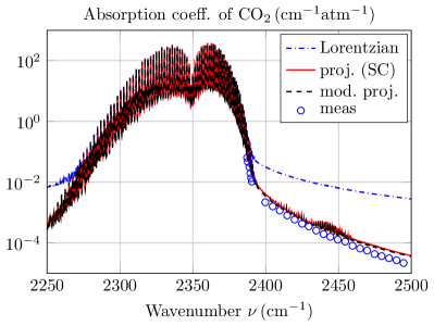
Figure 1: Relative absorption coefficient for the $\nu_{3}$ $\mathrm{CO}_{2}$-band in dry air at $T=20$$\mathrm{\,{}^{\circ}C}$ and total pressure $p=1$$\mathrm{\,atm}$. The blue dashdotted line (Lorentzian) indicates the sum of isolated Lorentzian lines, the red solid line (proj. (SC)) the basic projection method and the black dashed line (mod. proj.) the modified projection method. The blue rings (meas) indicate the corresponding measurement data which have been visually interpreted from [2, Fig. 2].

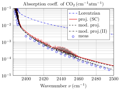
Figure 2: Same plot as in Fig. 1 focusing on the far wing at 2385-2500$\mathrm{\,cm^{-1}}$. Here, the black dashdotted line (mod. proj.(II)) corresponds to a small 0.5$\mathrm{\,\%}$ increase of the line coupling transfer rates where $\widehat{v}_{\mathrm{s}}^{\prime}=1.005\cdot\widehat{v}_{\mathrm{s}}^{\mathrm{ls}\prime}$.

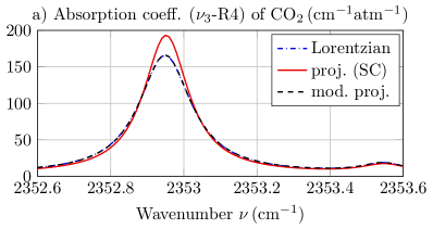
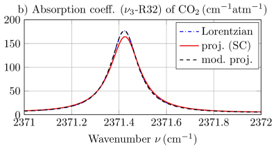
Figure 3: Same plot as in Fig. 1 focusing on the rotational R4 and R32 lines of the $\nu_{3}$ R-branch, respectively. Here, the modified projection (mod. proj.) is virtually coincident with the adequate Lorentzian, and the basic SC method is in error.

It can now be observed in Figs. 1 and 2 how the modified projection method is able to mimic and even improve the prediction of the basic projection (SC) method in the far wing region at the same time as the prediction of the modified method is virtually coincident with the adequate Lorentzian close to the center of isolated lines where the basic SC method is in error, cf., Fig. 3. It should finally be noted that the basic projection (SC) method can not be successfully scaled in the same way as the modified projection method. In this example, it turns out that a similar scaling of the SC method by $\widehat{v}_{\mathrm{s}}^{\prime}=0.6\cdot\widehat{v}_{\mathrm{s}}^{\mathrm{ls}\prime}$ (40 % decrease of $\widehat{v}_{\mathrm{s}}^{\mathrm{ls}\prime}$) will give the adequate far wing correction, but the line center resonances will then be completely destroyed. This is of course due to the fact that the scaling of the SC method (31) affects the diagonal elements as well as the line coupling transfer rates, whereas a similar scaling of the modified projection method (34) does only affect the line coupling transfer rates and which therefore has a very minor effect on the line centers.

V-B The $\mathrm{O}_{2}$-$\mathrm{H}_{2}\mathrm{O}$ millimeter-band

In Fig. 4 is shown the modeled millimeter range absorption of moist air at sea level where both the basic (proj. (SC)) as well as the modified projection method (mod. proj.) indicate results which are seemingly almost identical with the predictions made in [47, Fig. 4-6a on p. 124]. Here, the temperature is $T=15$$\mathrm{\,{}^{\circ}C}$ (288$\mathrm{\,K}$), the total pressure is $1$$\mathrm{\,atm}$ and the radiatively active molecules consist of 21$\mathrm{\,\%}$ oxygen and a water vapor content corresponding to 60$\mathrm{\,\%}$ humidity. In this computation we have also included the water vapor continuum absorption (the black dotted line) calculated as a combination of the MPM87 and MPM93 empirical models as proposed by Rosenkranz [48]. Here, the total absorption coefficient is given by $\alpha=\alpha_{\mathrm{line}}+\alpha_{\mathrm{cont}}$ where $\alpha_{\mathrm{line}}=N\sigma_{\mathrm{a}}$ is the usual line contribution of the radiator based on expressions like (76) and (78), $N$ its number density and where the continuum contribution is given by the following expression

$$\alpha_{\mathrm{cont}}=f^{2}\left(\frac{300}{T}\right)^{3}\left(C_{\mathrm{f}}p_{\mathrm{f}}p_{\mathrm{s}}+C_{\mathrm{s}}p_{\mathrm{s}}^{2}\right)$$ (83)

where $f$ is frequency in $\mathrm{\,GHz}$, $T$ temperature in $\mathrm{\,K}$ and $p_{\mathrm{f}}$ and $p_{\mathrm{s}}$ the partial pressure of air and water vapor, respectively, both in $\mathrm{\,kPa}$. The coefficient for foreign (air) broadening is $C_{\mathrm{f}}=2.38\cdot 10^{-7}$ (MPM87) and for self (water vapor) broadening $C_{\mathrm{s}}=7.8\cdot 10^{-6}\left(\frac{300}{T}\right)^{4.5}$ (MPM93), both in $\mathrm{\,dB/km/GHz^{2}/kPa^{2}}$.

In Fig. 4, we can now observe that the Lorentzian model is giving excess absorption, and in particular in between the two resonances of oxygen at 60$\mathrm{\,GHz}$ and 120$\mathrm{\,GHz}$, respectively, as well as in the upper wing of the latter. This discrepancy is alleviated by both of the present line mixing methods. In Figs 5 a) and b) are shown the corresponding close up views of the oxygen 60$\mathrm{\,GHz}$ resonance and the water vapor resonance at 183.3$\mathrm{\,GHz}$, respectively. It may be noticed here that the corresponding experimental value of the 60$\mathrm{\,GHz}$ peak absorption of dry air at 1$\mathrm{\,atm}$ and 15$\mathrm{\,{}^{\circ}C}$ is very close to 15$\mathrm{\,dB/km}$, cf., [49, Fig. 2]. As can be seen in these plots, the modified projection method follows closely the basic projection method (SC) in the oxygen band at 60$\mathrm{\,GHz}$ where lines overlap and line mixing is adequate. However, in the water vapor band at 183.3$\mathrm{\,GHz}$ the modified projection method follows instead tightly the Lorentzian where the dominating rotational line of water is virtually isolated and the basic SC method is in error.

In Fig. 6 is finally shown the modeling results for the 183.3$\mathrm{\,GHz}$ absorption band of an $\mathrm{N}_{2}$-$\mathrm{H}_{2}\mathrm{O}$ mixture at $T=23$$\mathrm{\,{}^{\circ}C}$ (296$\mathrm{\,K}$), total pressure $1$$\mathrm{\,atm}$ and water vapor pressure $p_{\mathrm{s}}=1/76$$\mathrm{\,atm}$ (10 torr). The modeling results are compared to measured data according to [50, Fig. 10 on p. 420]. As we can see here, the measured values are in fact closest to the Lorentzian model. We should remember, however, that this is in the wings of an isolated line. And it makes sense since the MPM87/93 parameters used above have been calibrated for the sum of Lorentzian lines, cf., [48, Eq. (4)], and line mixing typically reduces the absorption in the wings. However, the discrepancy is not very large and the MPM87/93 water vapor continuum model together with the proposed modified projection method appears to provide a useful model for millimeter waves taking line mixing effects into account, as illustrated in Figs. 4 through 6.

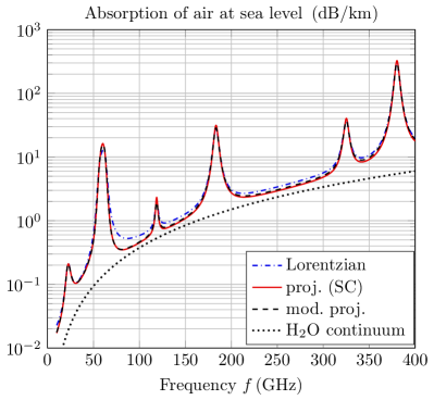
Figure 4: Absorption of moist air in the millimeter range at $T=15$$\mathrm{\,{}^{\circ}C}$, total pressure $p=1$$\mathrm{\,atm}$ and 60$\mathrm{\,\%}$ humidity. As before, the blue dashdotted line (Lorentzian) indicates the sum of isolated Lorentzian lines, the red solid line (proj. (SC)) the basic projection method and the black dashed line (mod. proj.) the modified projection method. The contribution from the water vapor continuum absorption is indicated by the black dotted line.

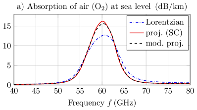
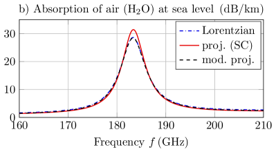
Figure 5: Same plot as in Fig. 4 focusing on a) the oxygen 60$\mathrm{\,GHz}$ band and b) the water vapor 183$\mathrm{\,GHz}$ band, respectively. Notice that the modified projection method follows the basic projection (SC) method in the oxygen band where line mixing is important, but it follows instead the Lorentzian close to the dominating isolated water vapor line at 183.3$\mathrm{\,GHz}$ where the SC method is largely deviating.

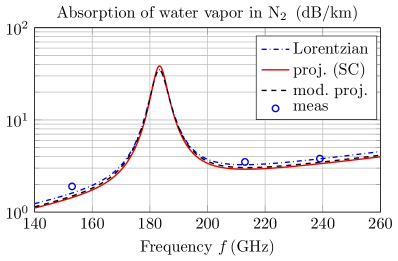
Figure 6: Absorption of an $\mathrm{N}_{2}$-$\mathrm{H}_{2}\mathrm{O}$ mixture at $T=23$$\mathrm{\,{}^{\circ}C}$, total pressure $1$$\mathrm{\,atm}$ and water vapor pressure $p_{\mathrm{s}}=1/76$$\mathrm{\,atm}$ (10 torr). The blue rings (meas) indicate measurements according to [50, Fig. 10 on p. 420].

VI Summary

A modified projection approach to line mixing has been presented which is based on a simple adjustment of the strong collision (SC) method introduced by Bulanin, Dokuchaev, Tonkov and Filippov. It has been demonstrated how basically any desired isolated line model encompassing uncorrelated collisions can be used as diagonal elements of the collisional relaxation matrix, at the same time as the SC line coupling transfer rates can be retained and optimally scaled to provide a proper far wing behavior. The method thus provides a simple and flexible compromise towards a unified treatment for all species in all parts of the spectrum.

In particular, by following the ideas of [7, 2], it is possible to express explicitly an exact solution to the line mixing problem in the case of uncorrelated collisions, pure pressure broadening and velocity independent broadening and shifts parameters. To include Doppler broadening one can readily apply the first order Rosenkranz approximation. Notably, within the present context with uncorrelated collisions and line independent Dicke narrowing, the Rosenkranz approximation will also allow the diagonal elements of the relaxation matrix to depend on speed and where analytical results exist with the quadratically speed dependent parameters associated with the Hartmann-Tran (HT) profile [19].

The method has been illustrated by using numerical examples including comparisons to published measured data in two specific cases concerning the absorption of carbon dioxide in its infrared $\nu_{3}$ ro-vibrational band at 2349$\mathrm{\,cm^{-1}}$, as well as of atmospheric water vapor and oxygen in relevant millimeter bands up to 400$\mathrm{\,GHz}$.

-A Integrals involving the Faddeeva function

Some of the important integral relationships involving the Maxwell-Boltzmann distribution as well as the Faddeeva function used in this paper are summarized below. The Faddeeva function is an entire function defined by

$$w(z)=\mathrm{e}^{-z^{2}}\mathrm{erfc}(-\mathrm{i}z)$$ (84)

where $\mathrm{erfc}(z)$ is the complementary error function defined by $\mathrm{erfc}(z)=\frac{2}{\sqrt{\pi}}\int_{z}^{\infty}\mathrm{e}^{-t^{2}}\mathrm{d}t$, see e.g., [51, Eq. (7.2.1) – (7.2.3)]. The Faddeeva function is of fundamental importance and very convenient to use in spectroscopic modeling due to the vast literature that is available on the theory, algorithms and computer codes for its efficient numerical evaluation, see e.g., [52, 53, 54, 55, 20]. The Maxwell-Boltzmann velocity distribution is given by $f(\bm{v})=(\sqrt{\pi}\widetilde{v})^{-3}\mathrm{e}^{-(v/\widetilde{v})^{2}}$ where $v=|\bm{v}|$, $\widetilde{v}=\sqrt{2k_{\mathrm{B}}T/\mu_{\mathrm{r}}}$ is the most probable speed, $k_{\mathrm{B}}$ the Boltzmanns constant, $T$ the temperature and $\mu_{\mathrm{r}}$ the mass of the radiator, cf., [56, Chapt. 5].

The first integral of interest here is the standard result

$$\int_{\bm{v}}f(\bm{v})\mathrm{e}^{-\mathrm{i}\bm{k}\cdot\bm{v}t}\mathrm{d}\bm{v}=\mathrm{e}^{-(k\widetilde{v}t/2)^{2}},$$ (85)

where $\bm{k}=k\hat{\bm{k}}$ is the wave vector associated with the incident radiation, see e.g., [16]. The integral identity (85) can readily be obtained by a substitution to spherical coordinates and is valid for all $t\in\mathbb{R}$.

By completing the squares in the exponent and employing the definition of the complementary error function, one can also derive the following Fourier-Laplace transform

$$\int_{0}^{\infty}\mathrm{e}^{-(k\widetilde{v}t/2)^{2}}\mathrm{e}^{\mathrm{i}\omega t}\mathrm{d}t=\frac{\sqrt{\pi}}{k\widetilde{v}}w\left(\frac{\omega}{k\widetilde{v}}\right),$$ (86)

which is valid for all $\omega\in\mathbb{C}$. Another useful integral identity can also be derived by inserting the result (85) into (86) and changing the order of integration to yield

$$\int_{\bm{v}}\frac{f(\bm{v})\mathrm{d}\bm{v}}{\mathrm{i}\bm{k}\cdot\bm{v}-\mathrm{i}\omega}=\frac{\sqrt{\pi}}{k\widetilde{v}}w\left(\frac{\omega}{k\widetilde{v}}\right),$$ (87)

but which is now valid only for $\mathrm{Im}\{\omega\}>0$. The latter restriction is usually not a problem since the resulting right-hand side can be analytically extended to the whole complex plane. An important example is the relation

$$\frac{1}{\pi}\mathrm{Re}\left\{\frac{\sqrt{\pi}}{k\widetilde{v}}w\left(\frac{\omega}{k\widetilde{v}}\right)\right\}=\frac{1}{\sqrt{\pi}k\widetilde{v}}\mathrm{e}^{-\omega^{2}/k^{2}\widetilde{v}^{2}}$$ (88)

where $\omega\in\mathbb{R}$, and which is a well known formula for Doppler broadening, cf., e.g., [16, 3, 20]. The integral identities (85), (86) and (87) are standard integrals which are employed in many papers, such as e.g., [19, 25].

References

- [1] N. N. Filippov, V. P. Ogibalov, and M. V. Tonkov, “Line mixing effect on the pure absorption in the 15 region,” J. Quant. Spectrosc. Radiat. Transfer, vol. 72, pp. 315–325, 2002.
- [2] M. V. Tonkov and N. N. Filippov, “Collision Induced Far Wings of and Bands in IR Spectra,” Camy-Peyret C., Vigasin A.A. (eds) Weakly Interacting Molecular Pairs: Unconventional Absorbers of Radiation in the Atmosphere. NATO Science Series (Series IV: Earth and Environmental Sciences), vol. 27, pp. 125–136, 2003.
- [3] J.-M. Hartmann, C. Boulet, and D. Robert, Collisional effects on molecular spectra. Laboratory experiments and models, consequences for applications, 2nd ed. Amsterdam: Elsevier, 2021.
- [4] A. B. Dokuchaev, N. N. Filippov, and M. V. Tonkov, “Line interference in rotational-vibrational band of in the strong interaction approximation,” Physica Scripta, vol. 25, pp. 378–380, 1982.
- [5] M. O. Bulanin, A. B. Dokuchaev, M. V. Tonkov, and N. N. Filippov, “Influence of line interference on the vibration-rotation band shapes,” J. Quant. Spectrosc. Radiat. Transfer, vol. 31, no. 6, pp. 521–543, 1984.
- [6] N. N. Filippov and M. V. Tonkov, “Semiclassical analysis of line mixing in the infrared bands of and ,” J. Quant. Spectrosc. Radiat. Transfer, vol. 50, no. 1, pp. 111–125, 1993.
- [7] M. V. Tonkov, N. N. Filippov, Y. M. Timofeyev, and A. V. Polyakov, “A simple model of the line mixing effect for atmospheric applications: Theoretical background and comparison with experimental profiles,” J. Quant. Spectrosc. Radiat. Transfer, vol. 56, no. 5, pp. 783–795, 1996.
- [8] “HITRANonline. The HITRAN Database. https://hitran.org.”
- [9] “HITRANonline. Definitions and units: Line-by-line parameters. https://hitran.org/docs/definitions-and-units/.”
- [10] L. S. Rothman and et al, “The HITRAN molecular spectroscopic database and HAWKS (HITRAN atmospheric workstation): 1996 edition,” J. Quant. Spectrosc. Radiat. Transfer, vol. 60, no. 5, pp. 665–710, 1998.
- [11] M. Šimečková, D. Jacquemart, L. S. Rothman, R. R. Gamache, and A. Goldman, “Einstein -coefficients and statistical weights for molecular absorption transitions in the HITRAN database,” J. Quant. Spectrosc. Radiat. Transfer, vol. 98, pp. 130–155, 2006.
- [12] I. E. Gordon and et al, “The HITRAN2020 molecular spectroscopic database,” J. Quant. Spectrosc. Radiat. Transfer, vol. 277, pp. 1–82, 2022.
- [13] K. N. Liou, An introduction to atmospheric radiation. London, UK: Academic Press, 2002.
- [14] A. Berk and F. Hawes, “Validation of MODTRAN 6 and its line-by-line algorithm,” J. Quant. Spectrosc. Radiat. Transfer, vol. 203, pp. 542–556, 2017.
- [15] S. Nordebo, “Uniform error bounds for fast calculation of approximate Voigt profiles,” J. Quant. Spectrosc. Radiat. Transfer, vol. 270, p. 107715, 2021.
- [16] S. G. Rautian and I. I. Sobel’man, “The effect of collisions on the Doppler broadening of spectral lines,” Soviet Physics Uspekhi, vol. 9, no. 5, pp. 701–716, 1967.
- [17] H. Tran and J.-M. Hartmann, “An isolated line-shape model based on the Keilson and Storer function for velocity changes. I. Theoretical approaches,” J. Chem. Phys., vol. 130, p. 094301, 2009.
- [18] N. H. Ngo, H. Tran, and R. R. Gamache, “A pure isolated line-shape model based on classical molecular dynamics simulations of velocity changes and semi-classical calculations of speed-dependent collisional parameters,” J. Chem. Phys., vol. 136, p. 154310, 2012.
- [19] N. Ngo, D. Lisak, H. Tran, and J.-M. Hartmann, “An isolated line-shape model to go beyond the Voigt profile in spectroscopic databases and radiative transfer codes,” J. Quant. Spectrosc. Radiat. Transfer, vol. 129, pp. 89–100, 2013.
- [20] J. Tennyson and et al, “Recommended isolated-line profile for representing high-resolution spectroscopic transitions (IUPAC Technical Report),” Pure Appl. Chem., vol. 86, pp. 1931–1943, 2014.
- [21] B. Lance, G. Blanquet, J. Walrand, and J.-P. Bouanich, “On the speed-dependent hard collision lineshape models: Application to perturbed by ,” J. Mol. Spectrosc., vol. 185, pp. 262–271, 1997.
- [22] A. S. Pine, “Asymmetries and correlations in speed-dependent Dicke-narrowed line shapes of argon-broadened ,” J. Quant. Spectrosc. Radiat. Transfer, vol. 62, pp. 397–423, 1999.
- [23] E. W. Smith, J. Cooper, W. R. Chappell, and T. Dillon, “An impact theory for Doppler and pressure broadening. I. General theory,” J. Quant. Spectrosc. Radiat. Transfer, vol. 11, pp. 1547–1565, 1971.
- [24] ——, “An impact theory for Doppler and pressure broadening. II. Atomic and molecular systems,” J. Quant. Spectrosc. Radiat. Transfer, vol. 11, pp. 1567–1576, 1971.
- [25] R. Ciuryło and A. S. Pine, “Speed-dependent line mixing profiles,” J. Quant. Spectrosc. Radiat. Transfer, vol. 67, pp. 375–393, 2000.
- [26] A. C. Kolb and H. Griem, “Theory of line broadening in multiplet spectra,” Physical Review, vol. 111, no. 2, pp. 514–521, 1958.
- [27] M. Baranger, “General impact theory of pressure broadening,” Physical Review, vol. 112, no. 3, pp. 855–865, 1958.
- [28] R. G. Gordon, “Semiclassical theory of spectra and relaxation in molecular gases,” J. Chem. Phys., vol. 45, no. 5, pp. 1649–1655, 1966.
- [29] ——, “On the pressure broadening of molecular multiplet spectra,” J. Chem. Phys., vol. 46, no. 2, pp. 448–455, 1967.
- [30] P. W. Rosenkranz, “Shape of the 5 mm oxygen band in the atmosphere,” IEEE Trans. Antennas Propagat., vol. 23, no. 4, pp. 498–506, 1975.
- [31] F. Rohart, H. Mäder, and H. W. Nicolaisen, “Speed dependence of rotational relaxation induced by foreign gas collisions: Studies on by millimeter wave coherent transients,” J. Chem. Phys., vol. 101, no. 8, pp. 6475–6486, 1994.
- [32] C. D. Boone, K. A. Walker, and P. F. Bernath, “Speed-dependent Voigt profile for water vapor in infrared remote sensing applications,” J. Quant. Spectrosc. Radiat. Transfer, vol. 105, pp. 525–532, 2007.
- [33] A. S. Pine and T. Gabard, “Speed-dependent broadening and line mixing in perturbed by and from multispectrum fits,” J. Quant. Spectrosc. Radiat. Transfer, vol. 66, pp. 69–92, 2000.
- [34] S. Vasilchenko, T. Delahaye, S. Kassi, A. Campargue, R. Armante, H. Tran, and D. Mondelain, “Temperature dependence of the absorption of the R(6) manifold of the 2 band of methane in air in support of the MERLIN mission,” J. Quant. Spectrosc. Radiat. Transfer, vol. 298, p. 108483, 2023.
- [35] A. S. Pine and V. N. Markov, “Self- and foreign-gas-broadened lineshapes in the band of ,” J. Mol. Spectrosc., vol. 228, pp. 121–142, 2004.
- [36] A. S. Pine and T. Gabard, “Multispectrum fits for line mixing in the band Q branch of methane,” J. Mol. Spectrosc., vol. 217, pp. 105–114, 2003.
- [37] A. S. Pine, “Speed-dependent line mixing in the band Q branch of methane,” J. Quant. Spectrosc. Radiat. Transfer, vol. 224, pp. 62–77, 2019.
- [38] J. Domysławska, S. Wójtewicz, K. Bielska, S. Bilicki, R. Ciuryło, and D. Lisak, “Line mixing in the oxygen B band head,” J. Chem. Phys., vol. 156, no. 084301, 2022.
- [39] C. Boulet and J.-M. Hartmann, “Toward measurements of the speed-dependence of line-mixing,” J. Quant. Spectrosc. Radiat. Transfer, vol. 262, p. 107510, 2021.
- [40] R. G. Gordon, “Theory of the width and shift of molecular spectral lines in gases,” J. Chem. Phys., vol. 44, no. 8, pp. 3083–3089, 1966.
- [41] D. Robert and L. Galatry, “Infrared absorption of diatomic polar molecules in liquid solutions,” J. Chem. Phys., vol. 55, no. 5, pp. 2347–2359, 1971.
- [42] R. A. Horn and C. R. Johnson, Matrix Analysis. Cambridge University Press, 1985.
- [43] A. S. Pine, “Line mixing sum rules for the analysis of multiplet spectra,” J. Quant. Spectrosc. Radiat. Transfer, vol. 57, no. 2, pp. 145–155, 1997.
- [44] D. Robert, J. M. Thuet, J. Bonamy, and S. Temkin, “Effect of speed-changing collisions on spectral line shape,” Physical Review A, vol. 47, no. 2, pp. R771–R773, 1993.
- [45] A. V. Domanskaya, N. N. Filippov, N. M. Grigorovich, and V. Tonkov, “Modelling of the rotational relaxation matrix in line-mixing effect calculations,” Molecular Physics, vol. 102, no. 16–17, pp. 1843–1850, 2004.
- [46] J. M. Mendel, Lessons in digital estimation theory. Englewood Cliffs, New Jersey: Prentice-Hall, Inc., 1987.
- [47] M. A. Richards, J. A. Scheer, and W. A. Holm, Principles of Modern Radar. SciTech Publishing, Edison, NJ., 2010, vol. I: Basic Principles.
- [48] P. W. Rosenkranz, “Water vapor microwave continuum absorption: A comparison of measurements and models,” Radio Sci., vol. 33, no. 4, pp. 919–928, 1998.
- [49] D. Makarov, M. Tretyakov, and P. Rosenkranz, “60-GHz oxygen band: Precise experimental profiles and extended absorption modeling in a wide temperature range,” J. Quant. Spectrosc. Radiat. Transfer, vol. 112, no. 9, pp. 1420–1428, 2011.
- [50] A. Bauer, M. Godon, J. Carlier, and Q. Ma, “Water vapor absorption in the atmospheric window at 239 GHz,” J. Quant. Spectrosc. Radiat. Transfer, vol. 53, no. 4, pp. 411–423, 1995.
- [51] F. W. J. Olver, D. W. Lozier, R. F. Boisvert, and C. W. Clark, NIST Handbook of mathematical functions. New York: Cambridge University Press, 2010.
- [52] B. H. Armstrong, “Spectrum line profiles: The Voigt function,” J. Quant. Spectrosc. Radiat. Transfer, vol. 7, pp. 61–88, 1967.
- [53] F. Schreier, “The Voigt and complex error function: A comparison of computational methods,” J. Quant. Spectrosc. Radiat. Transfer, vol. 48, no. 5/6, pp. 743–762, 1992.
- [54] ——, “Optimized implementations of rational approximations for the Voigt and complex error function,” J. Quant. Spectrosc. Radiat. Transfer, vol. 112, pp. 1010–1025, 2011.
- [55] S. M. Abrarov and B. M. Quine, “Efficient algorithmic implementation of the Voigt/complex error function based on exponential series approximation,” Appl. Math. Comput., vol. 218, pp. 1894–1902, 2011.
- [56] S. J. Blundell and K. M. Blundell, Concepts in thermal physics. New York: Oxford University Press Inc., 2010.