Rethinking matching-based
few-shot action recognition

Abstract

Few-shot action recognition, i.e. recognizing new action classes given only a few examples, benefits from incorporating temporal information. Prior work either encodes such information in the representation itself and learns classifiers at test time, or obtains frame-level features and performs pairwise temporal matching. We first evaluate a number of matching-based approaches using features from spatio-temporal backbones, a comparison missing from the literature, and show that the gap in performance between simple baselines and more complicated methods is significantly reduced. Inspired by this, we propose Chamfer++, a non-temporal matching function that achieves state-of-the-art results in few-shot action recognition. We show that, when starting from temporal features, our parameter-free and interpretable approach can outperform all other matching-based and classifier methods for one-shot action recognition on three common datasets without using temporal information in the matching stage.

Project page: https://jbertrand89.github.io/matching-based-fsar

1 Introduction

Recognizing actions within videos is essential for analyzing trends, enhancing broadcasting experience, or filtering out inappropriate content. However, collecting and annotating enough video examples to train supervised models can be prohibitively time-consuming. It is therefore desirable to recognize new action classes with as few labeled examples as possible. This is the premise behind the task of few-shot learning, where models learn to adapt to a set of unseen classes for which only a few examples are available. In video action recognition, additional challenges arise from the temporal dimension. Recognition methods need to capture the scene’s temporal context and temporal dynamics.

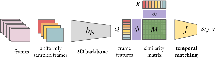
(a)

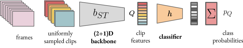
(b)

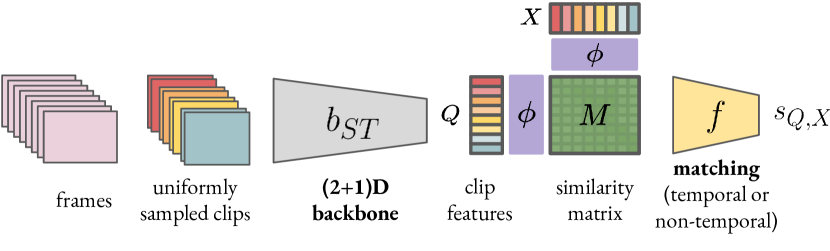
(c)

Figure 1: Different ways of using temporal information in few-shot action recognition. Temporal information is utilized: a) during matching (existing matching-based methods) b) in the backbone with a classifier (existing classifier-based methods, e.g. [33]) c) in the backbone with a matching step (this paper).

One family of approaches is formed by matching-based methods [3, 21, 36, 27] where each test example or “query” is compared against all support examples of a class to infer a class confidence score. Most existing matching-based methods use frame-level representations, i.e. a 2D convolutional backbone that takes a frame as input, and a feature set is formed by encoding multiple frames. Feature extraction is followed by matching the query feature set $Q$ to the support example set $X$, and a similarity $s_{Q,X}$ between the two is computed. This process is depicted in Figure 1(a). Although each feature represents an individual frame and cannot capture temporal information, the feature sets are usually temporal sequences, and the matching process can exploit such information.

Another family of approaches is formed by methods that learn a conventional linear classifier at test time, i.e. using the handful of examples available. In this case, any temporal context has to be incorporated in the representation, as shown in Figure 1(b). As a representative example, Xian et al. [33] adopt the spatio-temporal R(2+1)D architecture [28], where the input is a video clip, i.e. a sequence of consecutive frames, and convolutions across the temporal dimension enable the features to encode temporal information. Following findings in few-shot learning [31, 5], Xian et al. further abandon episodic training and instead fine-tune a pre-trained backbone using all training examples of the base classes. Using strong temporal features and by simply learning a linear classifier at test time, they report state-of-the-art results for few-shot action recognition.

Motivated by the two families of approaches presented above, we introduce a new setup depicted in Figure 1(c) that aims at answering the following questions:

1. Do matching-based methods still have something to offer for few-shot action recognition given strong temporal representations? We level the playing field with respect to representations and evaluate a number of recent matching-based approaches using strong temporal representations. We find that such approaches perform better than training a classifier at test time.

2. Is temporal matching necessary when the features capture temporal information? We show that matching-based methods invariant to the temporal order in the feature sequence (non-temporal matching) are performing as good as the ones that do use it (temporal matching) on many common benchmarks.

Inspired by the findings above, we further introduce Chamfer++, a novel, parameter-free and interpretable matching approach that employs Chamfer matching and is able to achieve a new state-of-the-art for one-shot action recognition on three common benchmarks.

2 Related Work

In the image domain, several methods for few-shot classification are metric-learning-based [29, 23, 26, 6, 2] and use a k-nearest-neighbor classifier at test time. Despite the dominance of meta-learning-based methods in the area [9, 10, 13, 22, 18], several recent studies highlight the importance of starting from strong visual representations. It is shown [31, 5] that if one learns representations without meta-learning but using instead all available data from all base classes, simple nearest-neighbors [31] or parametric classifier [5] baselines work on-par or better than most methods on common benchmarks. Similar observations are made for few-shot learning in the video domain [33, 37, 36].

As with the image domain, most methods leverage meta-learning and are grouped into initialization-based [33, 37], metric-learning [35, 1, 3, 34, 21, 36] and generative-based [8, 33] methods. However, unlike the image domain, most methods for few-shot action recognition try to take into account the temporal dimension in the visual representations and/or during the matching process. In fact, most methods incorporate temporal matching [35, 3, 1, 16, 34, 21, 17]. The features are either extracted from single frames [35, 3, 21] or clips [1, 33, 34] where temporal information is already captured in the features.

Some matching methods explicitly aim for temporal alignment and estimate video-to-video similarity via an ordered temporal alignment score. OTAM [3] finds the optimal path on the temporal similarity matrix via a differentiable approximation of the Dynamic Time Warping (DTW) [20] algorithm, a method also used for alignment in other temporal tasks [4, 7]. Other methods like ARN [34] use spatio-temporal attention, while TA²N [17] proposes two-stage spatial-temporal alignment. TARN [1] uses temporal attention over clip sequences for alignment. During the training process, the attention parameters, together with the parameters from a subsequent recurrent network, are learned such that features are aligned between the query and a support video from the correct class.

Other methods like TRX [21] or PAL [36] do not explicitly seek alignment but rely on cross-attention mechanisms over the query and support features to perform temporal matching. In both cases, class-wise representations are constructed and matching is performed directly in a video-to-class manner. For TRX, class representations are adapted on-the-fly in a query-conditioned manner, while for PAL the query features are instead adapted to match pre-computed class-wise representations. In our study, we show how such direct video-to-class approaches are highly competitive when more than one videos per class are provided, but that video-to-video methods are superior and more efficient for the one-shot case.

Recently, a number of methods suggest that the meta-learning framework is not optimal for the representation learning phase. Following similar observations in the image classification domain [31, 5], some few-shot action recognition methods [33, 37, 36] learn their representation on the full train set and report higher performance on multiple benchmarks. As discussed in Section 3.2.3, we follow such methods, and use a strong representation learned on the entire train set as the starting point for our study on temporal matching.

3 Method

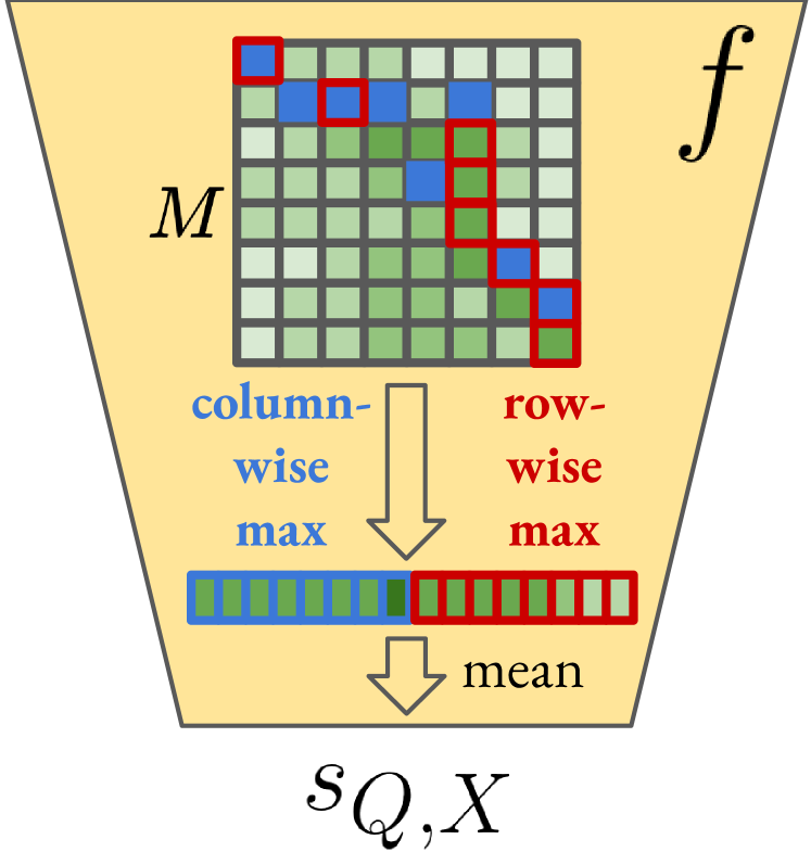
(a) Chamfer matching

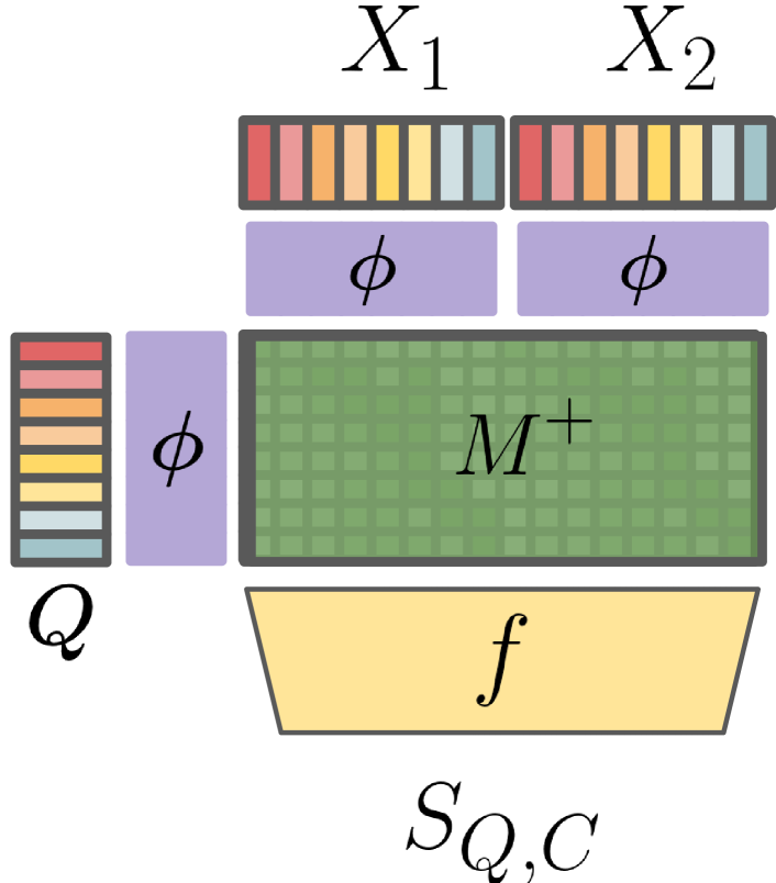
(b) Joint matching

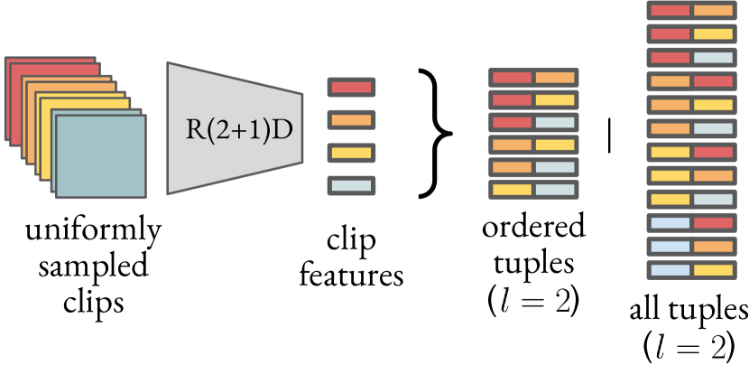
(c) Clip tuples

Figure 2: Details of the proposed matching approach. a) The Chamfer matching function $f_{QS}$ from Eq.(3). b) Jointly matching multiple examples per class (Chamfer+). c) using clip tuples as representation; one can use only ordered tuples or all tuples; in both cases, the matching part remains non-temporal, i.e. invariant to the temporal order of features.

We first present the video representation and the experimental protocol used in this work in Section 3.1. Then, we describe a framework to fairly compare matching-based and classifier-based approaches in Section 3.2.3 and propose a new matching function in Section 3.3.1. In the following, we refer to videos as examples and actions as classes.

3.1 Preliminaries

We describe the video representation that we use and the episodic protocol as formulated in the recent literature of few-shot video action recognition, which we follow in this work.

3.1.1 Video representation

A clip $c_{i}$ is a sequence of $L$ consecutive RGB frames in the form of a $L\times H\times W\times 3$ tensor. A deep video backbone $b$ takes a clip $c_{i}$ as input and maps it to a $d$-dimensional vector $\mathbf{q}_{i}=b(c_{i})\in^{d}$, named feature. We use the R(2+1)D backbone architecture [28] as in the work of Xian et al. [33], which uses efficient and effective separated spatio-temporal convolutions. A video $Q$ is represented by a set of clip features $Q=\{\mathbf{q}_{i}\}$. The clips are uniformly sampled over the temporal dimension, with possible overlap.

3.1.2 Episodic protocol

We adopt the commonly used setup [21, 3]. The classes of the train and test sets are non-overlapping and usually named base and novel classes, respectively. To simulate the limited annotated data, test episodes are randomly sampled from the test set. Each episode corresponds to a different classification task and comprises query and support examples for a fixed set of classes, where labels of support examples are known, while labels of query examples are unknown. Only $k$ labeled examples per class, also named shots, are available in the support set, with $k$ typically ranging from 1 to 5. The performance is evaluated via classification accuracy on the query examples averaged over all test episodes.

3.2 A common setup for classifier and matching-based approaches

We identify two dominant families of approaches proposed in the recent few-shot action recognition literature: the classifier-based and the matching-based methods . Unfortunately, discrepancies in setup and architecture between existing approaches make it difficult to compare them fairly. We propose to follow the same representation learning strategy and start from a common frozen backbone.

3.2.1 Classifier-based approaches

The classifier-based approaches  [33, 37] train the video representation using a classifier in the form of a linear layer. This is similar to the corresponding work on few-shot learning in the image domain [11].

Classifiers are trained using the whole dataset, but episodic training cannot guarantee to see all the examples because it is intractable to sample all the possible episodes. Xian et al. [33] depart from episodic training and propose a Two-stage Learning (TSL) process. During the first stage, a R(2+1)D video backbone and a classifier are learned jointly using all the labeled examples of the train set. During the second stage, the backbone remains fixed to avoid overfitting and a newly initialized classifier needs to be trained per test episode using the support examples.

In both stages, a linear classifier with a soft-max function denoted by $h:^{d}\rightarrow^{C}$, where C is the number of classes, is added to the output of the backbone. During the training stage, $C=C_{t}$ is equal to the number of all classes in the train set. During the second stage, $C=C_{f}$ is equal to the number of classes per test episode, usually $C_{f}=5$. Training is performed by optimizing the class probabilities $h(\mathbf{q}_{i})$ for each $\mathbf{q}_{i}\in Q$ with the cross-entropy loss ($\mathcal{L}_{cls}$), while inference is performed by sum-pooling of the classifier output across clips, i.e. $\sum_{\mathbf{q}_{i}\in X}h(\mathbf{q}_{i})$.

3.2.2 Matching-based approaches

The matching-based approaches estimate the similarity between the query and all the support examples of each class to obtain class probabilities. Training is performed on episodes sampled from the train set, which are meant to imitate the episodes of the test set.

Let $Q=\{\mathbf{q}_{i}\}$ and $X=\{\mathbf{x}_{i}\}$ be two videos with $|Q|=|X|=n$ and assume that $n$ is constant across videos. We form the temporal similarity matrix for the ordered video pair $(Q,X)$ denoted by $M_{Q,X}\in^{n\times n}$, or just $M$ for brevity, with elements $m_{ij}=\phi(\mathbf{q}_{i})^{\top}\phi(\mathbf{x}_{j})$, where $\phi:^{d}\rightarrow^{D}$ is a learnable projection head. The function $\phi$ consists of a linear layer, a layer normalization, and a $\ell_{2}$ normalization to guarantee bounded similarity values $m_{ij}$. When no linear projection is used, $\phi$ is equivalent to the identity mapping with an $\ell_{2}$ normalization. Each element $m_{ij}$ of the matrix $M$ can be seen as a temporal correspondence between clip $i$ of video $Q$ and clip $j$ of video $X$.

We consider the family of matching approaches that infer a video-to-video similarity $S_{Q,X}$, between video $Q$ and $X$, solely based on the matrix $M$, i.e. $S_{Q,X}=f(M)$, with $f:^{n\times n}\rightarrow$, named the matching function. The scalar $S_{Q,X}$ should be high if the two videos depict the same action. By definition, the result of function $f$ only depends on the strength and position of the pairwise similarities $m_{ij}$ and does not directly depend on the features themselves. The function $f$ can either be hand-crafted or include learnable parts. A graphical overview of different matching approaches is given in the appendix as long as a more detailed description of them. Some matching functions use temporal information by leveraging the position, either absolute or relative, of the pairwise similarities $m_{ij}$. The matching functions that use temporal information are called temporal, whereas the others are called non temporal.

The pairwise video-to-video similarities between query and support examples are averaged per class to obtain class probabilities . During training, the class probabilities are optimized with the cross-entropy loss ($\mathcal{L}_{cls}$). Inference is also performed by estimating the similarity between query and all support examples. This is a form of a k-nearest-neighbor classifier.

3.2.3 A common starting point

We follow the training stage of TSL [33] to learn the R(2+1)D backbone parameters using all the annotated examples. We freeze this backbone, and treat the resulting model as a feature extractor. This is our starting point for both classifier-based and matching-based approaches which enable us to fairly compare the two families of approaches. Specifically, matching-based methods only learn the feature projection function $\phi$ and the matching parameters when needed in a test-agnostic way. Unlike classifier-based methods, which need to train a classifier for every testing episode, matching-based approaches require no learning or adaptation at test time. They only need the pairwise matching between the query and each one of the support examples.

3.3 Chamfer++

We propose a new matching function, Chamfer++, which is non-temporal and achieves top performance while being parameter-free and intuitive. It is an extension of Chamfer similarity (Figure 2(a)) with joint-matching over multiple shots (Figure 2(b)) applied in conjunction with clip-feature-tuples instead of clip features (Figure 2(c)). This section details its main components.

3.3.1 Chamfer

The Chamfer matching function $f_{Q}$ is given by

$$f_{Q}(M):=\frac{1}{n}\sum_{i}\max_{j}m_{ij}.$$ (1)

Each clip of the query example is matched with its most similar one within the clips of a support example to produce the score between this specific query clip and this support example. The final video-to-video similarity is the average of all the query clip scores. The Chamfer matching function implies that each clip sampled from the query example contributes to the similarity score by matching its closest clip in the support example. One can transpose the temporal similarity matrix and derive the symmetric process where each clip from the support example needs to match a query clip. Then the matching function becomes

$$f_{S}(M):=\frac{1}{n}\sum_{j}\max_{i}m_{ij}.$$ (2)

Chamfer-S is equivalent to the Chamfer on the transposed matrix $M^{\top}$. Summing the two gives a symmetric Chamfer variant, where all clips from both the query and the support example are required to match:

$$f_{QS}(M):=f_{Q}(M)+f_{S}(M).$$ (3)

We refer to this symmetric variant as simply Chamfer matching in the context of few-shot action recognition. In the following, we also refer to Chamfer-Q as query-based and Chamfer-S as support-based.

3.3.2 Joint-matching

As discussed in Section 3.2.2, the standard option to compute the query-to-class probabilities is by averaging the pairwise similarity score between the query example and all the support examples belonging to the class. Instead, we propose to match all support examples jointly. We concatenate the temporal similarity matrices between the query and all support examples. It creates the joint temporal similarity matrix $M^{+}$, with $M^{+}\in^{n\times kn}$. Then, we compute the matching function on top of $M^{+}$ to obtain video-to-class similarity $S_{Q,c}:=s(M^{+})$. We evaluate the impact of this newly proposed joint-matching versus the standard single-matching in Section 4.3. We refer to this variant as Chamfer+ in the rest of the manuscript.

3.3.3 Clip tuples

Besides the case where each clip feature is matched independently, Perret et al. [21] additionally propose matching feature tuples. Inspired by this, we extend Chamfer to enable matching of clip feature tuples formed by any clip subset of fixed length $l$. A clip feature tuple $\mathbf{t}^{l}$ contains $l$ clip features, non-necessarily consecutive, but with the same relative order as in $Q=\{\mathbf{q}_{i}\}$. For example, $\mathbf{t}^{2}=\{(q_{i},q_{j\neq i)}\}$. Each clip feature tuple is concatenated and fed to the learnable projection head $\phi:^{ld}\rightarrow^{D}$. The resulting temporal similarity matrix is $M^{++}\in^{n^{\prime}\times kn^{\prime}}$, with $n^{\prime}={n\choose l}$. The clip tuples are sub-sequence representations on top of single-clip representations. By definition, clip tuples add additional temporal information to the representation. But the matching function remains non-temporal.

We also define non-temporally ordered clip tuples $\mathbf{t}_{all}^{l}$ as the permutations of $l$ clip features. For example, $\mathbf{t}_{all}^{2}=\{(q_{i},q_{j\neq i)}\}$. The resulting temporal similarity matrix is $M^{++}\in^{n^{\prime}\times kn^{\prime}}$ with $n^{\prime}=n!$. The comparison between ordered and all tuples is presented in Table 3 and the appendix. In the following, the extension of Chamfer matching that jointly matches multiple shots and uses clip tuples is referred to as Chamfer++. Unless otherwise stated, we use ordered clip tuples.

4 Experiments

We report results on the three most commonly used benchmarks for few-shot action recognition, i.e. Kinetics-100 [35], Something-Something V2 (SS-v2) [12], and UCF-101 [24]. Kinetics-100 and UCF-101 contain videos collected from YouTube. Each video is trimmed to include only one coarse-grained human action such as “playing trumpet” or “reading book”. SS-v2 contains egocentric videos where humans were instructed to perform predefined actions such as “pushing something from left to right” or “dropping something into something”.

We use the train/val/test splits from [35] for all three datasets, containing 64/12/24 classes, respectively. We learn the parameters of the R(2+1)D backbone using the train split, similar to [33]. For matching-based approaches, we learn the projection $\phi$ together with any learnable parameters in the matching function $f$ using episodic training also on the train split. We use the val split for hyper-parameter tuning and early stopping.

We evaluate on the common 1-shot and 5-shot setups. Unless otherwise stated, we use 5-way classification tasks. Training episodes are randomly sampled from the train set. We use the same fixed, predefined set of 10k test episodes sampled from the test set for all methods (prior work samples them randomly). We always evaluate three trained models and report mean and standard deviation.

4.1 Implementation details

We use the publicly available code for TSL for training the backbone as well as for reproducing the TSL method. We adapt the public TRX codebase for learning parameters of the matching function and testing, as well as for reproducing the TRX and OTAM methods.

Table 1: Few-shot action recognition results. All methods are trained and evaluated by us and use the same R(2+1)D [28] backbone. TSL [33] learns a classifier at each episode during testing. All the rest are pairwise matching-based methods and are split into two categories: non-temporal, i.e. invariant to the temporal order of features, and temporal. ^† denotes Chamfer++ matching using all tuples. Best (second-best) results are presented in bold (underlined).

Method	SS-v2		Kinetics-100		UCF-101
	1-shot	5-shot	1-shot	5-shot	1-shot	5-shot
Parametric classifier
TSL [33]	60.6 $\pm 0.1$	79.9 $\pm 0.0$	93.6 $\pm 0.0$	98.0 $\pm 0.00$	97.1 $\pm 0.0$	99.4 $\pm 0.0$
Non-temporal matching
Mean	65.8 $\pm 0.0$	79.1 $\pm 0.1$	95.5 $\pm 0.0$	98.1 $\pm 0.1$	97.6 $\pm 0.2$	98.9 $\pm 0.1$
Max	65.0 $\pm 0.2$	79.0 $\pm 0.0$	95.3 $\pm 0.1$	98.3 $\pm 0.0$	97.9 $\pm 0.1$	98.9 $\pm 0.0$
Chamfer++†	67.0 $\pm 0.3$	80.8 $\pm 0.1$	96.2 $\pm 0.1$	98.4 $\pm 0.1$	97.8 $\pm 0.1$	99.2 $\pm 0.1$
Chamfer++	67.8 $\pm 0.2$	81.6 $\pm 0.1$	96.1 $\pm 0.1$	98.3 $\pm 0.0$	97.7 $\pm 0.0$	99.3 $\pm 0.0$
Temporal matching
Diagonal	66.7 $\pm 0.1$	80.1 $\pm 0.0$	95.3 $\pm 0.1$	98.1 $\pm 0.1$	97.6 $\pm 0.2$	99.0 $\pm 0.0$
Linear	66.6 $\pm 0.1$	80.1 $\pm 0.2$	95.5 $\pm 0.1$	98.1 $\pm 0.0$	97.6 $\pm 0.1$	98.9 $\pm 0.0$
OTAM [3]	67.1 $\pm 0.0$	80.2 $\pm 0.2$	95.9 $\pm 0.0$	98.4 $\pm 0.1$	97.8 $\pm 0.1$	99.0 $\pm 0.0$
TRX-{2,3} [21]	65.5 $\pm 0.1$	81.8 $\pm 0.2$	93.4 $\pm 0.2$	97.5 $\pm 0.0$	96.6 $\pm 0.0$	99.5 $\pm 0.0$
ViSiL [16]	67.7 $\pm 0.0$	81.3 $\pm 0.0$	95.9 $\pm 0.0$	98.2 $\pm 0.0$	97.8 $\pm 0.2$	99.0 $\pm 0.1$

Learning the backbone parameters. We start from the publicly available 34-layer R(2+1)D backbone provided by the TSL codebase. This model is pre-trained on the large Sports-1M dataset [15]. We follow [33] and use a SGD optimizer with a constant learning rate of 0.001 for the backbone and 0.1 for the 64-class linear layer. We perform early-stopping using the 64-class validation dataset. Then, we use the backbone as a feature extractor to extract features from $n=8$ uniformly sampled clips. The input video clips are composed of 16 consecutive RGB frames with a spatial resolution of 112x112, and the dimensionality of the resulting feature vector is $d=512$.

Training matching-based methods. We train the matching-based methods on the training episodes with an SGD optimizer and a constant learning rate of 0.001 for every method except for TRX where we use a learning rate of 0.01. Similar to prior work [3, 21], we select the best model using early stopping by measuring performance on the validation set. We learn the projection $\phi$ jointly with any matching parameters. We set the projection dimension to $D=1152$ if not stated otherwise. This is equivalent to the dimensionality that TRX[21] uses for its attention layer. We train all the matching methods with the cross-entropy loss that uses softmax with a learnable temperature $\tau$.

Learning classifiers for TSL. Instead of pairwise matching, TSL [33] learns classifiers at every test episode, using all available support examples. To reproduce TSL we follow [33] and use the Adam optimizer with a constant learning rate of 0.01 for 10 epochs. The original TSL approach uses $n=10$ clips at test-time, but we set this number to $n=8$ to keep it the same with all matching methods for a fair comparison. Preliminary experiments show that this choice doesn’t affect the performance of TSL at all.

Data augmentation. During training, videos are augmented with random cropping. We uniformly sample 8 clips from each video with temporal jittering, i.e. randomly perturb the starting point of each clip. Additionally, for the Kinetics-100 dataset, we also use random horizontal flipping as data augmentation. Since it is important for SS-v2 to distinguish between left-to-right and right-to-left, we do not use horizontal flipping for that dataset. We only apply a center crop for videos during validation and testing.

4.2 Results

(a) SS-v2

(b) Kinetics-100

(c) UCF-101

Figure 3: One-shot performance for different backbones, types of matching, or use of parametric classifiers. The different colors account for the different backbones. The different shapes account for the type of matching. ^† denotes methods reproduced in this study.

In this section, we report and analyse our results. We first discuss the gains from using temporal representations and the comparison between matching-based and classifier approaches. We then discuss the use of temporal information during matching and present results when varying the number of classes per classification task (test episode). Finally, we compare Chamfer++ to other recently published methods and show that our approach achieves state-of-the-art performance.

Frame or clip-based features? We start by evaluating a number of recent matching-based methods over temporal features. This is an important comparison that is missing from the current few-shot action recognition literature. In Figure 3, we report one-shot performance for a number of matching methods under a common evaluation setup and using both frame-based (ResNet, blue points) and clip-based (R(2+1)D, orange points) features.

We clearly see that using a spatio-temporal backbone significantly boosts accuracy by more than 10% on all datasets. Interestingly, this is also true for the Kinetics-100 and the UCF-101 datasets that are known to be more biased towards spatial context [14]. Even for this case where context is important, we see that temporal dynamics remain a valuable cue for few-shot action recognition. It is worth noting that the performance on UCF-101 and Kinetics-100 appears to be saturated when using spatio-temporal representations.

Pairwise matching or classifiers? Matching-based methods and classifiers are compared in Table 1 and Figure 3. All results in the table are computed under a common framework, i.e. all methods share representations from an R(2+1)D backbone and are tested on the same set of episodes. We see that for all setups and datasets, several matching approaches outperform TSL. In the 1-shot regime, most matching-based methods outperform TSL.

Table 2: Comparison with the state-of-the-art. Unless otherwise stated, we report results as presented in the corresponding papers. ^† denotes results reproduced in [37] and ^‡ denotes results generated by us. Best (second-best) results are presented in bold (underlined).

Method	Clip-based	Venue	SS-v2		Kinetics-100		UCF-101
	backbone		1-shot	5-shot	1-shot	5-shot	1-shot	5-shot
Classifier-based
Baseline [37]		BMVC21	40.8	59.2	69.5	84.4	-	-
Baseline + [37]		BMVC21	46.0	61.1	74.6	86.6	-	-
TSL [33]	✓	PAMI21	59.1	80.1	92.5	97.8	94.8	-
TSL ‡	✓	PAMI21	60.6	79.9	93.6	98.0	97.1	99.4
Matching-based
CMN++ † [35, 37]		ECCV18	40.6	51.9	65.9	82.7	-	-
ARN [34]	✓	ECCV20	-	-	63.7	82.4	66.3	83.1
OTAM [3]		CVPR20	48.8	52.3	73.0	85.8	-	-
PAL [36]		BMVC21	46.4	62.6	74.2	87.1	85.3	95.2
TRX-{1} [21]		CVPR21	38.8	60.6	63.6	85.2	-	-
TRX-{2,3} [21]		CVPR21	42.0	64.6	63.6	85.9	-	96.1
STRM-{2} [27]		CVPR22	-	70.2	-	91.2	-	98.1
TA2N [17]		AAAI22	47.6	61.0	72.8	85.8	81.9	95.1
MTFAN  [32]		CVPR22	45.7	60.4	74.6	87.4	84.8	95.1
HyRSM [30]		CVPR22	54.3	69.0	73.7	86.1	-	-
TAP  [25]		CVPR22	45.2	63.0	-	-	83.9	95.4
CPM  [19]		ECCV22	59.6	-	81.0	-	79.0	-
Chamfer++ ‡	✓		67.8	81.6	96.1	98.3	97.7	99.3

How useful is temporal matching? No significant difference in performance is observed between temporal and non-temporal matching approaches, as highlighted in Table 1 and Figure 3. On the Kinetics-100 and UCF-101 datasets, where action classes are generally coarser and highly dependent on context [14], most methods we tested perform similarly well. Simply using $f(M)=\max_{ij}m_{ij}$ is enough to achieve top performance for UCF-101, while the proposed Chamfer++ outperforms all other methods on Kinetics-100. When it comes to the finer-grained SS-v2 dataset, we see that, although most non-temporal matching methods lag behind the temporal ones for the 1-shot case, the proposed Chamfer++ method achieves the highest performance without temporal matching. For 5-shot action recognition, TRX, ViSiL, and Chamfer++ perform similarly well, with the last being parameter-free, more intuitive, and faster.

(a) SS-v2 dataset. 1-shot (left) and 5-shot (right)

(b) Kinetics-100 dataset. 1-shot (left) and 5-shot (right)

(c) UCF-101 dataset. 1-shot (left) and 5-shot (right)

Figure 4: Impact of the number of classes per episode ($C_{f}$) on three datasets.

Varying the number of classes in an episode. Figure 4 shows the performance when extending the case of $C_{f}=5$ classes to the maximum number of classes, $C_{f}=24$, in the 1-shot and 5-shot regime. We see that for 1-shot the proposed non-temporal Chamfer++ method highly outperforms TRX and the classifier-based TSL method in all datasets.

Table 3: Chamfer++ variants.

Method	$l$	Joint	Tupl.	1-shot	5-shot
Chamfer-Q	1			65.7 $\pm 0.1$	79.7 $\pm 0.1$
Chamfer-S	1			65.3 $\pm 0.1$	79.1 $\pm 0.2$
Chamfer	1			66.9 $\pm 0.1$	80.0 $\pm 0.2$
Chamfer+	1	✓		66.9 $\pm 0.1$	80.7 $\pm 0.2$
Chamfer++	2	✓	all	67.1 $\pm 0.1$	80.8 $\pm 0.2$
Chamfer++	2	✓	ord.	67.7 $\pm 0.1$	81.4 $\pm 0.2$
Chamfer++	3	✓	all	67.0 $\pm 0.3$	80.8 $\pm 0.1$
Chamfer++	3	✓	ord.	67.8 $\pm 0.2$	81.6 $\pm 0.1$

Comparison to the state-of-the-art. In Table 2, we compare the performance of the proposed Chamfer++ with the corresponding numbers reported in many recent few-shot action recognition papers. Although there is no direct comparison between all these methods, i.e., no common setup or backbones, we present all results jointly to show the overall progress in the task.

4.3 Chamfer matching ablation and interpretability

In Table 3, we present an ablative study with the 1-shot performance of all the different variants of Chamfer++ we discuss in Section 3.3 on the SS-v2 dataset. Combining support-based and query-based Chamfer matching helps learn a better projection $\phi$, while both joint matching and the use of clip tuples improve performance compared to the vanilla variant. Although using ordered clip tuples improves for 1-shot on SS-v2, overall, we see in Table 1 that using all or ordered tuples results in more or less similar performance.

Which are the most informative clips? As we presented in Section 3.1, we sample and encode a set of clips to represent each video. Not all clips are, however, equally valuable for the matching process. To provide some insight and illustrate the proposed method’s interpretability, we study a qualitative example from SS-v2 in Figure 5. When matching the query video to the two support videos belonging to the same class (top), we see many clip-to-clip correspondences with high magnitudes (shown as thicker lines). This is not the case when matching to the support videos belonging to a negative class (bottom) and we can only see a single strong correspondence. Upon better inspection, we saw that the motion of picking up the object in the fourth clip of the query video does exhibit a left-to-right motion locally that matches the negative class. Nevertheless, the other correspondences are weaker. Leveraging more than one clip helps Chamfer matching to disambiguate while, at the same time, its inherent selectivity makes it more robust against noisy correspondences. This example illustrates that not all the clip correspondences are equally valuable to compute a video-to-video similarity metric. The matching step is a dynamic way to select the most informative clip correspondences that highlight the similarity between two videos.

Figure 5: Matching a query video (middle) from “Picking something up” with two support videos of “Picking something up” (top) and two support videos of “Pulling something from left to right” (bottom). Each video consists of 8 clips with 16 frames each. We only show the first and last frames on top of each other in the figure (see project page for animated versions). In grey, we draw the correspondences between the query and the support videos selected by Chamfer (query-based). In red, we draw the correspondence selected by max (single strongest correspondence). Line thickness corresponds to the pairwise similarity.

5 Conclusion

A number of recent few-shot learning papers are abandoning the meta-learning protocol for representation learning [31, 37, 5, 33] and show that adaptation from the best possible features leads to better performance. In the quest for rapid adaptation at test time, we also adopt this setup and show that, given strong visual representations, simple matching-based methods are really effective and able to beat both classifier-based and more complex matching-based approaches on many common benchmarks for few-shot action recognition. We further show that temporal information in the matching provides no particular benefit compared to the ability to learn or adapt from strong temporal features, and introduce an intuitive matching-based method that is not only parameter-free but also easy to visualize and interpret.

Acknowledgements. This work was supported by Naver Labs Europe, by Junior Star GACR GM 21-28830M, and by student grant SGS23/173/OHK3/3T/13. The authors would like to sincerely thank Toby Perrett and Dima Damen for sharing their early code and supporting us, Diane Larlus for insightful conversations, feedback, and support, and Zakaria Laskar, Monish Keswani, and Assia Benbihi for their feedback.

Appendix 0.A Appendix

In this appendix, we present more formally the matching functions used as baselines for our study in (Section 0.A.1), as well as extra experiments that study the impact of different hyper-parameters and present results of different task setups (Section 0.A.2).

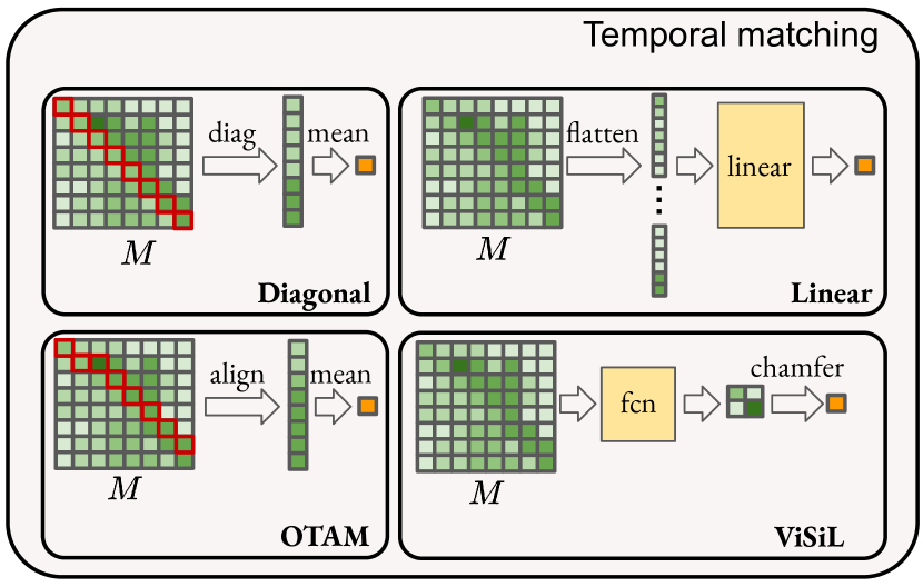
(a)

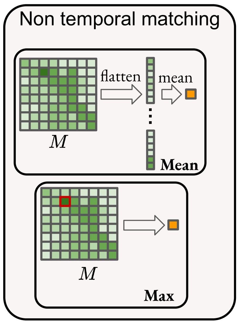
(b)

Figure 6: Matching functions on the temporal similarity matrix $M$. We show how each method estimates a scalar video-to-video similarity given the input pairwise similarity matrix. The functions can be classified as a) temporal or b) non-temporal whether they use the temporal position of the features or not.

0.A.1 Baseline matching functions

In this section, we describe the different matching functions used as our study’s baseline, and depicted in Figure 6. Some matching functions use temporal information by leveraging the absolute or relative position of the pairwise similarities $m_{ij}$. The matching functions that use temporal information are called temporal whereas the others are called non-temporal.

0.A.1.1 Temporal matching functions.

We provide a list of the temporal matching functions implemented in this study as baselines. Some of them were already introduced in prior work.

Diagonal (Diag) is used as a baseline in prior work [3]. It is given by $s(M)=\displaystyle\nicefrac{{\sum_{ij}m_{ii}}}{{n}}$. It assumes temporally aligned video pairs.

OTAM [3] uses and extends Dynamic Time Warping [20] to find an alignment path on $M$ over which similarities are averaged to produce the video-to-video similarity. A differentiable variant is used for training.

Flatten+FC (Linear) is a simple baseline we use to learn temporal matching by flattening $M$ and feeding it to a Fully Connected (FC) layer without bias and with a single scalar output. Video-to-video similarity is therefore given by $s(M)=\sum_{ij}w_{ij}m_{ij}$, where $w_{ij}$ are learnable parameters which are $n^{2}$ in total.

ViSiL [16] is an approach originally introduced for the task of video retrieval. We apply it to few-shot action recognition for the first time. A small Fully Convolutional Network (FCN) is applied on $M$. Its output is a filtered temporal similarity matrix, and the Chamfer similarity is applied on it. The filtering is performed according to the small temporal context captured by the small receptive field of this network.

0.A.1.2 Non-temporal matching functions.

We provide a list of the non-temporal matching functions that were implemented in this study as baselines.

Mean is used as a baseline in prior work [3]. It is given by $s(M)=\displaystyle\nicefrac{{\sum_{ij}m_{ij}}}{{n^{2}}}$. It supposes all the clip pairs should contribute equally to the similarity score.

Max is used as a baseline in prior work [3]. It is given by $s(M)=\max_{ij}m_{ij}$. It supposes that selecting the best matching clip pair is enough to recognize the action.

0.A.2 Additional ablations and impact of hyper-parameters

In this section, we present additional ablations to evaluate the impact of the feature projection head, the ordering of the tuples, and the number of examples per class used in the support set. We also report the impact of using the different variants for the Kinetics-100 and UCF-101 datasets.

Table 4: Impact of learning a feature projection on performance of matching-based methods. ^† denotes hand-crafted matching methods, i.e. no training is performed for the cases where a feature projection is not learned.

Method	Learned	SS-v2		Kinetics-100
	Proj.	1-shot	5-shot	1-shot	5-shot
Max†		63.40	75.80	94.90	97.50
Max	✓	64.97	78.97	95.27	98.30
		($\uparrow$ 1.57)	($\uparrow$ 3.17)	($\uparrow$ 0.37)	($\uparrow$ 0.80)
Chamfer++ (l=3)†		64.50	79.50	94.10	98.10
Chamfer++ (l=3)	✓	67.83	81.60	96.10	98.30
		($\uparrow$ 3.33)	($\uparrow$ 2.10)	($\uparrow$ 2.00)	($\uparrow$ 0.20)
Mean†		61.40	75.40	92.50	97.50
Mean	✓	65.77	79.13	95.53	98.10
		($\uparrow$ 4.37)	($\uparrow$ 3.73)	($\uparrow$ 3.03)	($\uparrow$ 0.60)
OTAM [3]†		63.70	76.40	93.70	97.90
OTAM [3]	✓	67.10	80.23	95.93	98.37
		($\uparrow$ 3.40)	($\uparrow$ 3.83)	($\uparrow$ 2.23)	($\uparrow$ 0.47)

Table 5: Impact of the dimension size of the feature projection head for Chamfer++ using ordered-tuples and $l=3$.

Method	$D$	SS-v2		Kinetics-100
		1-shot	5-shot	1-shot	5-shot
Chamfer++ (l=3)		64.5 $\pm 0.0$	79.5 $\pm 0.0$	94.1 $\pm 0.0$	98.1 $\pm 0.0$
Chamfer++ (l=3)	512	67.3 $\pm 0.2$	81.2 $\pm 0.0$	95.9 $\pm 0.1$	98.2 $\pm 0.1$
Chamfer++ (l=3)	1024	67.8 $\pm 0.3$	81.3 $\pm 0.1$	96.1 $\pm 0.2$	98.3 $\pm 0.0$
Chamfer++ (l=3)	1152	67.8 $\pm 0.2$	81.6 $\pm 0.1$	96.1 $\pm 0.1$	98.3 $\pm 0.0$
Chamfer++ (l=3)	2048	67.9 $\pm 0.0$	81.8 $\pm 0.2$	96.1 $\pm 0.1$	98.3 $\pm 0.0$

0.A.2.1 The impact of the projection layer

for matching methods is validated in Table 4. The performance is consistently improved on all setups and methods by including and learning a projection layer. Although the backbone is trained with TSL on the same meta-train set, the projection layer allows features and values in the temporal similarity matrix to better align with each matching process.

0.A.2.2 Projection head dimension.

To match the work from [21], we set the projection dimension to $D=1152$. This section evaluates the effect of using different values for $D$. The results are reported in Table 5. A minimum value of $D=1024$ seems enough and could be used for future experiments.

0.A.2.3 Impact of using different variants

Table 6: Chamfer++ variants on the three datasets: UCF-101, Kinetics-100 and SS-v2.

Method	$l$	Joint	Tupl.	SS-v2		Kinetics-100		UCF-101
				1-shot	5-shot	1-shot	5-shot	1-shot	5-shot
Chamfer-Q	1			65.7 $\pm 0.1$	79.7 $\pm 0.1$	95.5 $\pm 0.1$	98.1 $\pm 0.1$	97.8 $\pm 0.1$	99.0 $\pm 0.1$
Chamfer-S	1			65.3 $\pm 0.1$	79.1 $\pm 0.2$	95.4 $\pm 0.0$	98.2 $\pm 0.1$	97.7 $\pm 0.2$	98.9 $\pm 0.1$
Chamfer	1			66.9 $\pm 0.1$	80.0 $\pm 0.2$	96.0 $\pm 0.1$	98.3 $\pm 0.1$	97.9 $\pm 0.2$	99.0 $\pm 0.1$
Chamfer+	1	✓		66.9 $\pm 0.1$	80.7 $\pm 0.2$	96.0 $\pm 0.1$	98.2 $\pm 0.1$	97.9 $\pm 0.2$	99.2 $\pm 0.1$
Chamfer++	2	✓	all	67.1 $\pm 0.1$	80.8 $\pm 0.2$	96.1 $\pm 0.1$	98.3 $\pm 0.1$	97.8 $\pm 0.1$	99.2 $\pm 0.1$
Chamfer++	2	✓	ord.	67.7 $\pm 0.1$	81.4 $\pm 0.2$	96.1 $\pm 0.1$	98.3 $\pm 0.1$	97.9 $\pm 0.1$	99.2 $\pm 0.1$
Chamfer++	3	✓	all	67.0 $\pm 0.3$	80.8 $\pm 0.1$	96.2 $\pm 0.2$	98.4 $\pm 0.0$	97.8 $\pm 0.1$	99.2 $\pm 0.1$
Chamfer++	3	✓	ord.	67.8 $\pm 0.2$	81.6 $\pm 0.1$	96.1 $\pm 0.1$	98.3 $\pm 0.0$	97.7 $\pm 0.0$	99.3 $\pm 0.0$

We report the accuracy for the different variants of Chamfer++ for the Kinetics-100 and UCF-101 datasets in Table 6. As for SS-v2, both variants improve performances compared to the vanilla approach.

0.A.2.4 Impact of ordering the clip-tuples

In this section, we evaluate the impact of using ordered clip feature tuples $\mathbf{t}^{l}$ versus using all the clip feature tuples $\mathbf{t}_{all}^{l}$. The comparison between ordered tuples and all tuples is presented in Table 7. On the SS-v2 dataset, using ordered clip feature tuples boosts the accuracy. On the Kinetics-100 and the UCF-101 datasets, using ordered tuples doesn’t provide a boost and can even slightly harm the performance. Since the number of tuples is significantly lower when they are in order, using the ordered clip feature tuples is preferable.

Table 7: Impact of using ordered clip feature tuples vs all the features for different values of $l$.

Method	$l$	Ordered	SS-v2		Kinetics-100		UCF-101
		Tuples	1-shot	5-shot	1-shot	5-shot	1-shot	5-shot
Chamfer++	2		67.10	80.80	96.10	98.33	97.80	99.23
Chamfer++	2	✓	67.73	81.40	96.10	98.33	97.87	99.23
			($\uparrow$ 0.63)	($\uparrow$ 0.80)	($\uparrow$ 0.00)	($\uparrow$ 0.00)	($\uparrow$ 0.07)	($\uparrow$ 0.00)
Chamfer++	3		67.03	80.83	96.17	98.37	97.77	99.23
Chamfer++	3	✓	67.83	81.60	96.10	98.30	97.73	99.27
			($\uparrow$ 0.80)	($\uparrow$ 0.77)	($\downarrow$ 0.07)	($\downarrow$ 0.07)	($\downarrow$ 0.04)	($\uparrow$ 0.04)

0.A.2.5 Impact of the number of examples per class

The impact of $k$ is shown in Figure 0.A.2.5 by measuring performance for an increasing number of support examples per class while keeping the number of classes fixed, $C_{t}=C_{f}=5$. We observe that TSL and TRX have inferior performances for the low-shot regime, while their performance increases faster with the number of shots. In the low-regime, Chamfer-QS++ outperforms the other methods and still keeps some benefits while the number of shots increases.

Figure 7: Evolution of the accuracy with the number of examples per class in the support set for the three datasets.

References

- [1] Mina Bishay, Georgios Zoumpourlis, and I. Patras. Tarn: Temporal attentive relation network for few-shot and zero-shot action recognition. In BMVC, 2019.
- [2] Kaidi Cao, Maria Brbić, and Jure Leskovec. Concept learners for few-shot learning. In ICLR, 2021.
- [3] Kaidi Cao, Jingwei Ji, Zhangjie Cao, Chien-Yi Chang, and Juan Carlos Niebles. Few-shot video classification via temporal alignment. In CVPR, 2020.
- [4] Chien-Yi Chang, De-An Huang, Yanan Sui, Li Fei-Fei, and Juan Carlos Niebles. D3tw: Discriminative differentiable dynamic time warping for weakly supervised action alignment and segmentation. In CVPR, 2019.
- [5] Wei-Yu Chen, Yen-Cheng Liu, Zsolt Kira, Yu-Chiang Frank Wang, and Jia-Bin Huang. A closer look at few-shot classification. In ICLR, 2019.
- [6] Carl Doersch, Ankush Gupta, and Andrew Zisserman. Crosstransformers: spatially-aware few-shot transfer. In NeurIPS, 2020.
- [7] Mikita Dvornik, Isma Hadji, Konstantinos G Derpanis, Animesh Garg, and Allan Jepson. Drop-dtw: Aligning common signal between sequences while dropping outliers. In NeurIPS, 2021.
- [8] Sai Kumar Dwivedi, Vikram Gupta, Rahul Mitra, Shuaib Ahmed, and Arjun Jain. Protogan: Towards few shot learning for action recognition. In ICCVW, 2019.
- [9] Chelsea Finn, Pieter Abbeel, and Sergey Levine. Model-agnostic meta-learning for fast adaptation of deep networks. In ICML, 2017.
- [10] Chelsea Finn, Kelvin Xu, and Sergey Levine. Probabilistic model-agnostic meta-learning. In NeurIPS, 2018.
- [11] Spyros Gidaris and Nikos Komodakis. Dynamic few-shot visual learning without forgetting. In CVPR, 2018.
- [12] R. Goyal, S. Kahou, V. Michalski, J. Materzynska, S. Westphal, H. Kim, V. Haenel, I. Fruend, P. Yianilos, M. Mueller-Freitag, F. Hoppe, C. Thurau, I. Bax, and R. Memisevic. The "something something" video database for learning and evaluating visual common sense. In ICCV, 2017.
- [13] Erin Grant, Chelsea Finn, Sergey Levine, Trevor Darrell, and Thomas Griffiths. Recasting gradient-based meta-learning as hierarchical bayes. In ICLR, 2018.
- [14] De-An Huang, Vignesh Ramanathan, Dhruv Mahajan, Lorenzo Torresani, Manohar Paluri, Li Fei-Fei, and Juan Carlos Niebles. What makes a video a video: Analyzing temporal information in video understanding models and datasets. In CVPR, 2018.
- [15] Andrej Karpathy, George Toderici, Sanketh Shetty, Thomas Leung, Rahul Sukthankar, and Li Fei-Fei. Large-scale video classification with convolutional neural networks. In CVPR, 2014.
- [16] Giorgos Kordopatis-Zilos, Symeon Papadopoulos, Ioannis Patras, and Ioannis Kompatsiaris. Visil: Fine-grained spatio-temporal video similarity learning. In ICCV, 2019.
- [17] Shuyuan Li, Huabin Liu, Rui Qian, Yuxi Li, John See, Mengjuan Fei, Xiaoyuan Yu, and Weiyao Lin. Ta2n: Two-stage action alignment network for few-shot action recognition. In AAAI, 2022.
- [18] Yann Lifchitz, Yannis Avrithis, Sylvaine Picard, and Andrei Bursuc. Dense classification and implanting for few-shot learning. In CVPR, 2019.
- [19] Yifei Huang Lijin Yang and Yoichi Sato. Compound prototype matching for few-shot action recognition. In ECCV, 2022.
- [20] Meinard Müller. Dynamic time warping. Information Retrieval for Music and Motion, 2007.
- [21] Toby Perrett, Alessandro Masullo, Tilo Burghardt, Majid Mirmehdi, and Dima Damen. Temporal-relational crosstransformers for few-shot action recognition. In CVPR, 2021.
- [22] Andrei A. Rusu, Dushyant Rao, Jakub Sygnowski, Oriol Vinyals, Razvan Pascanu, Simon Osindero, and Raia Hadsell. Meta-learning with latent embedding optimization. In ICLR, 2019.
- [23] Jake Snell, Kevin Swersky, and Richard Zemel. Prototypical networks for few-shot learning. In NeurIPS, 2017.
- [24] Khurram Soomro, Amir Roshan Zamir, and Mubarak Shah. Ucf101: A dataset of 101 human actions classes from videos in the wild. In CRCV-TR-12-01, 2012.
- [25] Bing Su and Ji-Rong Wen. Temporal alignment prediction for supervised representation learning and few-shot sequence classification. In ICLR, 2022.
- [26] Flood Sung, Yongxin Yang, Li Zhang, Tao Xiang, Philip Torr, and Timothy Hospedales. Learning to compare: Relation network for few-shot learning. In CVPR, 2018.
- [27] Anirudh Thatipelli, Sanath Narayan, Salman Khan, Rao Muhammad Anwer, Fahad Shahbaz Khan, and Bernard Ghanem. Spatio-temporal relation modeling for few-shot action recognition. In CVPR, 2022.
- [28] Du Tran, Heng Wang, Lorenzo Torresani, Jamie Ray, Yann LeCun, and Manohar Paluri. A closer look at spatiotemporal convolutions for action recognition. In CVPR, 2018.
- [29] Oriol Vinyals, Charles Blundell, Timothy Lillicrap, koray kavukcuoglu, and Daan Wierstra. Matching networks for one shot learning. In NeurIPS, 2016.
- [30] Xiang Wang, Shiwei Zhang, Zhiwu Qing, Mingqian Tang, Zhengrong Zuo, Changxin Gao, Rong Jin, and Nong Sang. Hybrid relation guided set matching for few-shot action recognition. In CVPR, 2022.
- [31] Yan Wang, Wei-Lun Chao, Kilian Q Weinberger, and Laurens van der Maaten. Simpleshot: Revisiting nearest-neighbor classification for few-shot learning. arXiv preprint arXiv:1911.04623, 2019.
- [32] Jiamin Wu, Tianzhu Zhang, Zhe Zhang, Feng Wu, and Yongdong Zhang. Motion-modulated temporal fragment alignment network for few-shot action recognition. In CVPR, 2022.
- [33] Y. Xian, B. Korbar, M. Douze, L. Torresani, B. Schiele, and Z. Akata. Generalized few-shot video classification with video retrieval and feature generation. IEEE TPAMI, 2021.
- [34] Hongguang Zhang, Li Zhang, Xiaojuan Qi, Hongdong Li, Philip H. S. Torr, and Piotr Koniusz. Few-shot action recognition with permutation-invariant attention. In ECCV, 2020.
- [35] Linchao Zhu and Yi Yang. Compound memory networks for few-shot video classification. In ECCV, 2018.
- [36] Xiatian Zhu, Antoine Toisoul, Juan-Manuel Pérez-Rúa, Li Zhang, Brais Martinez, and Tao Xiang. Few-shot action recognition with prototype-centered attentive learning. In BMVC, 2021.
- [37] Zhenxi Zhu, Limin Wang, Sheng Guo, and Gangshan Wu. A closer look at few-shot video classification: A new baseline and benchmark. In BMVC, 2021.