Relative pose of three calibrated and partially calibrated cameras from four points using virtual correspondences

Abstract

We study challenging problems of estimating the relative pose of three cameras and propose novel efficient solutions to (1) the notoriously difficult configuration of four points in three calibrated views, known as the 4p3v problem, and (2) to the previously unsolved configuration of four points in three cameras with unknown shared focal length, i.e., the 4p3vf problem. Our solutions are based on the simple idea of generating one or two additional virtual point correspondences in two views by using the information from the locations of the four input correspondences in the three views. We generate such correspondences using either a very simple and efficient strategy where the new points are the mean points of three corresponding input points or using a simple neural network. The new solvers are efficient and easy to implement since they are based on existing efficient minimal solvers, i.e., the well-known 5-point and 6-point relative pose solvers and the P3P solver. Our solvers achieve state-of-the-art results on real data.

1 Introduction

Camera geometry estimation is crucial in many computer vision applications, e.g., visual navigation [51], structure-from-motion [55], augmented and mixed reality [9], self-driving cars [18], and visual localization [50].

Due to noise and outliers in input correspondences, the predominant way in camera geometry estimation is to use a hypothesis-and-test framework, e.g., RANSAC [16, 11, 48, 3]. For RANSAC-like methods, it is critical to estimate camera geometry using as few correspondences as possible since the number of RANSAC iterations (and, thus, its run-time) depends exponentially on the number of correspondences required for the model estimation.

Figure 1: Visualization of the 4p3v problem and our solution that is based on generating new virtual correspondence(s) (in red) between two views. This is done using coordinates of input point correspondences. Then the 4p3v problem is solved by existing efficient minimal solvers, i.e., the 5pt [38] and the P3P solvers [43].

Algorithms that solve camera geometry estimation problems using all available constraints and the minimum number of correspondences, such that the resulting system of equations has a finite number of solutions, are called minimal solvers, and the corresponding problems are called minimal problems. Minimal problems often result in complex systems of polynomial equations in several variables. After introducing algebraic-based methods [57, 26, 28, 30, 6] for generating efficient polynomial solvers to the computer vision community, solutions to many previously unsolved minimal problems were proposed

[58, 8, 36, 31, 27, 29, 60, 7]. Still, some problems result in equations for which state-of-the-art algebraic methods fail to generate a solver that is efficient and/or numerically stable.

In this paper, we study such challenging problems of estimating the relative pose of three cameras. These problems have attracted attention for a long time [20, 47, 33, 37, 1]. However, due to their complexity, they are still not considered fully solved. No efficient and practical solutions exist for most of the minimal configurations of point and line correspondences, as well as for partially calibrated cameras. One such configuration that is particularly interesting is the notoriously difficult configuration of four points in three views [47, 38]. This configuration is minimal for three cameras with an unknown shared focal length, i.e., the 4p3vf problem, and provides one more constraint than minimal for calibrated cameras, i.e., the 4p3v problem.

State-of-the-art algebraic and numerical methods are known to fail to generate efficient and numerically stable solutions to both the 4p3v and 4p3vf problems. The existing methods for solving the 4p3v problem for calibrated cameras are thus only approximate. By solving only for one (few) solutions from the 272 solutions of the system that describe the problem [21], and by discretely sampling the space of potential solutions [39], the existing 4p3v methods can often fail, i.e., the returned solution can be, in general, arbitrarily far from the geometrically correct solution. To decrease the failure rate, both methods [21, 39] require a lot of tuning and are not easy to re-implement.

In this paper, we propose a novel approach for solving both the calibrated 4p3v, as well as, the previously unsolved 4p3vf problem for cameras with an unknown shared focal length. Our solutions are based on the simple idea of generating new approximate point correspondence(s) between two of the three views. Such correspondences are generated using only the locations of the four triplets of input point correspondences. Since the generation of new points does not require information from the image itself (e.g., information about appearance or features in the image), new correspondences, in general, do not need to correspond to any physical 3D points in the scene. Thus, we call them virtual correspondences. Using virtual correspondences, we can efficiently solve the 4p3v and 4p3vf problems by first estimating the relative pose of the two cameras from five/six correspondences using efficient 5pt/6pt solvers [38, 59], and then registering the third camera using the P3P solver [43]. We call this combination of the 5pt/6pt relative pose and the P3P solver the 5pt+P3P and 6pt+P3P solvers.

Based on this idea, we propose two groups of novel solvers for the 4p3v and 4p3vf problems: (1) M-solvers (4p3v(M),4p3vf(M)): Solvers that use the mean points of three corresponding points detected in two views and potentially points in their vicinity ((M$\pm\delta$)-solvers) as new virtual point correspondences. (2) L-solvers (4p3v(L),4p3vf(L)): Solvers that, given four triplets of corresponding points in three views and a point in the first view, use a network to predict a corresponding point to this point in the second view, i.e., a virtual correspondence. While simple to implement, the novel solvers achieve state-of-the-art results for the 4p3v/4p3vf problems on real data.

The contributions of the paper are as follows:

• For the well-known challenging 4p3v problem for calibrated cameras, we propose two groups of novel solutions 4p3v(M)- and 4p3v(L)-based solvers. These solvers generate an additional virtual point correspondence(s) in two views by leveraging the locations of four input triplet correspondences. The new solvers achieve state-of-the-art results in terms of accuracy on real data. Compared to state-of-the-art solutions to the 4p3v problem [21, 39], which are non-trivial and difficult to re-implement such that they are numerically stable and fast, our new solutions, especially the 4p3v(M)-based solvers, can be easily implemented using existing efficient implementations of the 5pt solver [38] and the P3P solver [43].

• We provide the first efficient solutions to the previously unsolved 4p3vf problem for cameras with unknown equal focal lengths. Our novel 4p3vf(M)- and 4p3vf(L)-based solvers generate for each instance two virtual correspondences to solve the problem using the efficient 6pt [38] and the P3P solver [43]. Our novel solvers show the potential of the proposed idea of virtual correspondences to be applied to other camera geometry problems.

• We compare the proposed solvers, the state-of-the-art 4p3v solver [21], as well as “oracle”-based 4p3v/4p3vf solvers, with the baseline minimal 5pt+P3P and 6pt+P3P solvers. By evaluating all solvers on a large amount of real data as well as data with outliers, we discuss which minimal point configuration is potentially the most useful in which scenario.

  The source code of our solvers will be publicly available.

2 Related work

Estimating the relative pose of three cameras from a minimal number of point and line correspondences is known as an extremely challenging problem.

For three uncalibrated cameras, 6 point correspondences are necessary to estimate the trifocal tensor, with a solution known for a long time [46, 61]. Solutions to three minimal combinations of points and lines are presented in [40]. The minimal configuration using 9 lines is much more challenging and was solved only recently by Larsson et al. [30]. However, the final solver is far from practical as it performs elimination of a huge $16k\times 13k$ matrix and runs 17.8s.

For calibrated cameras, the configuration that attracts most of the attention is the configuration of four points in three views (the 4p3v problem). Note, that this is not a minimal configuration since it generates 12 constraints for 11 degrees-of-freedom (DoF) (see also Section 3). The 4p3v problem is known as being extremely difficult to solve. Several papers present mostly theoretical results [33, 37, 1]. For four triplets of exact points without noise, it is shown that the 4p3v problem has, in general, a unique solution [20, 47].

To the best of our knowledge, there are only two reasonably efficient solutions to the 4p3v problem reported in the literature. The first solver [39] is based on one-dimensional exhaustive search. In the paper, the authors derive several interesting theoretical results and show that the four point correspondences between two calibrated views constrain the epipole in each image to lie on a curve of degree ten. The solver performs a one-dimensional sweep of the curve of possible epipoles. For each potential epipole, it computes the relative pose of two cameras, registers the third camera using three triangulated points, and finally extracts the solution minimizing the reprojection error of the fourth point in the third view. The evaluation of the solver on one potential epipole is fast. Yet, to obtain reasonable precise and stable results, usually, 1,000 candidates need to be evaluated and even then, refinement at multiple local minima is required to improve the precision. The reported run-times of this solver were $1-12$ms depending on the number of searched points. There is no publicly available implementation for this solver and it is not easy to re-implement. As such, the literature does not compare against the solver in experiments. As an upper bound of the performance of [39], we compare against an oracle version using the true epipole.

The second efficient solver to the 4p3v problem was published only recently [21]. In this paper, the authors first transform the 4p3v problem to a minimal problem by considering a line passing through the last correspondence in the third view. The resulting system of equations is solved using an efficient Homotopy continuation (HC) method [15, 56]. To avoid computing large numbers of spurious solutions, an MLP-based classifier is trained. For a given problem $p$, it selects one or several starting problem-solution pairs (so-called anchors), such that the geometrically meaningful/correct solution of $p$ can be obtained by HC starting from this anchor. This strategy is fast, running $16.3\mu s$ on average per solution. At the same time, it has a high failure rate. The success rate of the 4p3v solver reported in [21] on two test datasets and data without noise is $26.3\%$. [21] do not show results of their solver in a real scenario, i.e., a RANSAC-like framework with noisy data. We provide such an evaluation in this paper.

Simple solutions to the 4p3v problem for orthographic and scaled orthographic views were presented in [63, 34]. In [34], the author suggested an iterative approach for updating to perspective views. However, he reported results only on a few synthetic instances. Even after spending a non-negligible amount of work and time (months) to make this update work, we were not able to get reasonable results on real data with general perspective cameras.

Minimal configurations of points and lines in three calibrated views were studied in [14, 24, 13], aiming to classify and derive the number of solutions for different configurations. Solutions to two minimal configurations of combinations of points and lines, the so-called Chicago and Cleveland problems, were proposed in [15]. These problems result in 216 respectively 312 solutions and are solved using HC methods [56]. Due to their complexity, the resulting solvers are not practical in real applications, with running times ranging from $0.66$s to $1.9$s.

Recently, a very efficient GPU implementation of the homotopy continuation method was used to solve minimal problems of four points in three views and six lines in three views for a generalized (non-central) camera [12].

In our solutions, we generate virtual correspondences. Virtual matches are also used in the literature of affine correspondences (AC) [42, 44, 45, 5]. There, points are sampled based on the affine feature geometry to generate point correspondences from affine ones. In our scenario, we are directly given point correspondences, without associated feature geometry, and we predict additional point matches.

3 Estimating the relative pose of three cameras

Let $N$ cameras observe a set of 3D points $\mathcal{P}$ and for each point $\mathbf{P}\in\mathcal{P}$, let $C_{\mathbf{P}}>1$ be the number of cameras that observe it. A necessary condition for a relative pose problem of $N$ calibrated cameras to be minimal is [15]

$$\sum_{\mathbf{P}\in\mathcal{P}}(2C_{\mathbf{P}}-3)=6N-7\enspace.$$ (1)

A configuration of points in $N=3$ views that satisfies the constraint (1) of a minimal problem is three points visible in all three cameras and two additional points visible in two of the three cameras. We will call this configuration $(5_{3},5_{3},3_{3})$, where the lower index on the position $i$ indicates how many from the image points sampled in the camera $i$ are visible in all three cameras.

The configuration of four points visible in all three cameras, i.e., the configuration $(4_{4},4_{4},4_{4})$, generates an over-constrained problem. In this case, we have one more constraint than DoF, i.e., in Eq. (1), we have $12>11$. A minimal solution would need to drop one constraint, e.g., by considering only a line passing through one of the points in the third view [21] or by considering a “half” point correspondence. Since, in practice, we always have full correspondences and sampling one less point in one view leads to an under-constrained problem, the configuration $(4_{4},4_{4},4_{4})$, is usually considered “minimal”.

For cameras with unknown common focal lengths, we have one more DoF. This means that, for $N=3$, the right-hand side of equation (1) equals to 12, resulting in $(6_{3},6_{3},3_{3})$ and $(4_{4},4_{4},4_{4})$ being minimal configurations.

3.1 Calibrated cameras

In this section, we describe solutions for three calibrated cameras. We start with one baseline solution for the minimal $(5_{3},5_{3},3_{3})$ configuration followed by novel solutions for the “minimal” $(4_{4},4_{4},4_{4})$ configuration.

5pt+P3P solver:  First, we review a simple baseline minimal solver for the configuration $(5_{3},5_{3},3_{3})$, i.e., the configuration where three points are visible in all three cameras and two additional points in two of the three cameras.

The 5pt+P3P solver first estimates the relative pose of two cameras from 5 image point correspondences using the efficient 5pt solver [38]. Next, the three points that are visible in all three views are triangulated. Finally, the third camera is registered using the three 2D-3D point correspondences and the well-known efficient P3P solver [43].

This solver is straightforward and it is based on efficient existing solvers [38, 43]. The 5pt+P3P solver is not novel. This solver and the $(5_{3},5_{3},3_{3})$ configuration was, e.g., mentioned in [14], where the authors present a classification of minimal problems for points and lines (partially) observed by three calibrated perspective cameras. However, the $(5_{3},5_{3},3_{3})$ configuration and the 5pt+P3P solver were only discussed from a theoretical point of view, aiming to report the number of solutions to this problem and not its practical performance. The 5pt+P3P solver is used by some researchers [38] and practitioners in their applications [49]. Nister et al. [39] showed that the 5pt+P3P solver performs better than their dedicated 4p3v solver. Still, the 5pt+P3P solver is not even used as a baseline for a comparison in papers that study the relative pose problem for three calibrated cameras [15, 21]. To our knowledge, the performance of this solver on real data and within state-of-the-art RANSAC frameworks in the context of the 4p3v problem has not been extensively studied. Our paper fills this gap in the literature.

Motivated by the efficient 5pt+P3P solver and the minimal $(5_{3},5_{3},3_{3})$ configuration, which, compared to the $(4_{4},4_{4},4_{4})$ configuration, leads to significantly simpler systems of polynomial equations, we next describe two groups of novel solvers to the calibrated 4p3v problem. These solvers efficiently solve the $(4_{4},4_{4},4_{4})$ configuration by generating a virtual point correspondence in the first two views, and thus solving it using the 5pt+P3P solver.

4p3v(M) solver:  Our first solver is based on a simple observation: If we fix the $5^{\text{th}}$ point in the first view to be the mean $\mathbf{m}^{1}$ of three points $\left\{\mathbf{x}_{i}^{1},\mathbf{x}_{j}^{1},\mathbf{x}_{k}^{1}\right\},\;i,j,k\in\left\{1,\dots,4\right\}$ in this view, then the mean point $\mathbf{m}^{2}$ of the corresponding three points $\left\{\mathbf{x}_{i}^{2},\mathbf{x}_{j}^{2},\mathbf{x}_{k}^{2}\right\}$ in the second view usually has a small epipolar error w.r.t. the ground truth relative pose. Thus $\mathbf{m}^{1}\leftrightarrow\mathbf{m}^{2}$ is usually a good approximation of a correct correspondence.

This can be considered as a surprising fact, since 4 (or actually 3) points in two views define an infinite number of camera poses that can observe these points. However, the reason this mean-point strategy works in practice comes from three simple facts and observations. (1) To generate a good correspondence, we only require that the point in the second view be reasonably close to the epipolar line defined by the mean point $\mathbf{m}^{1}$ in the first view, i.e., the 2D point does not need to correspond to one particular 3D point with a given depth. (2) The epipolar line defined by $\mathbf{m}^{1}$ passes through the triangle defined by the corresponding three points $\left\{\mathbf{x}_{i}^{2},\mathbf{x}_{j}^{2},\mathbf{x}_{k}^{2}\right\}$ in the second image. Therefore, the maximum distance of $\mathbf{m}^{2}$ in the second image from the epipolar line is bounded by the maximum distance of $\mathbf{m}^{2}$ from $\left\{\mathbf{x}_{i}^{2},\mathbf{x}_{j}^{2},\mathbf{x}_{k}^{2}\right\}$. (3) Three 3D points define a plane. If this plane is not observed under very oblique and different angles in two views, then the point on the 3D plane that projects on the mean point in the first image usually projects close to the mean point $\mathbf{m}^{2}$ in the second image. We support this observation by experiments on a large amount of synthetic and real data (cf. Sec. 4, mean-point strategy).

Motivated by these observations, our 4p3v(M) solver uses the mean points of three corresponding points detected in two views as a new $5^{\text{th}}$ point correspondence. The 4p3v problem is then solved using the 5pt+P3P solver.

4p3v(M$\pm\delta$) solver:  While the mean point correspondence used in the 4p3v(M) solver can provide a good approximation of a correct correspondence, such a correspondence can be noisy. In the 4p3v(M$\pm\delta$) solver, we thus, in addition to the mean point $\mathbf{m}^{2}=\left[x,y\right]$ of three points $\left\{\mathbf{x}_{i}^{2},\mathbf{x}_{j}^{2},\mathbf{x}_{k}^{2}\right\}$ in the second image, generate two additional points. These points are (1) $\mathbf{m}^{2}_{\delta}=\left[x\pm\delta,y\right]$ if the longest dimension of the triangle $\mathcal{T}^{2}=\Delta\left\{\mathbf{x}_{i}^{2},\mathbf{x}_{j}^{2},\mathbf{x}_{k}^{2}\right\}$ is in the x direction or (2) $\mathbf{m}^{2}_{\delta}=\left[x,y\pm\delta\right]$ if it is in the y direction. All three points, i.e., $\mathbf{m}^{2}$ and $\mathbf{m}^{2}_{\delta}$ are placed in correspondence with the mean point $\mathbf{m}^{1}$. The 4p3v(M$\pm\delta$) solver in the first step calls the 5pt solver [38] three times, with the $5^{th}$ correspondence being either $\mathbf{m}^{1}\leftrightarrow\mathbf{m}^{2}$ or $\mathbf{m}^{1}\leftrightarrow\mathbf{m}^{2}_{\delta}$. The results of these three 5pt solvers are collected to create hypotheses for the relative pose of the first two cameras inside RANSAC. The shift $\delta$ is selected relative to the size of the triangle $\mathcal{T}^{2}$.

4p3v(L) solver:  In our learning-based 4p3v(L) solver, instead of using the mean point correspondence, we use a network to predict this virtual correspondence. We use the fact that four triplets of points, in general, define a unique relative pose of three calibrated cameras. We train a network that given such four corresponding points in three views and a fixed 5${}^{\text{th}}$ point in the first view, it predicts a corresponding 5${}^{\text{th}}$ point in the second view.

We use a lightweight architecture with a backbone of shared MLP layers, similar to [10], such that each triplet of correspondences is processed independently. The input to our network is a $4\times 6$ matrix of 4 point correspondences containing the $x$ and $y$ coordinates in three views. In estimating the epipolar geometry, the order of the point correspondences does not matter. Thus, our network is designed to be permutation invariant in that input axis. The input is normalized as follows: We apply a rotation matrix to the points in each view independently, so that the mean point of the first three points is sent to $(0,0)$, and the fourth point is sent to $(0,y)$. Let $\mathbf{m}^{1},\mathbf{m}^{2}$, and $\mathbf{m}^{3}$ be the mean points of the three corresponding points in three views. We aim to predict the corresponding point of $\mathbf{m}^{1}$ in the second view. Let us denote this predicted point by $\mathbf{\tilde{m}}^{2}$, i.e., our $5^{th}$ virtual correspondence in the first two views will be $\mathbf{m}^{1}\leftrightarrow\mathbf{\tilde{m}}^{2}$. As suggested by the 4p3v(M) solver, $\mathbf{\tilde{m}}^{2}$ should be close to $\mathbf{m}^{2}$. Thus, we use the mean point $\mathbf{m}^{2}$ as the initialization of our network and predict a shift from $\mathbf{m}^{2}$.

Our loss function is the Sampson error $\mathcal{L}_{S}$ of the prediction to the epipolar line of $\mathbf{m}^{1}$ in the $2^{\text{nd}}$ view:

$$\mathcal{L}_{S}=\frac{{\mathbf{\tilde{m}}^{2^{\top}}}\mathbf{E}\mathbf{m}^{1}}{\sqrt{\lVert\mathbf{E}\mathbf{m}^{1}\rVert^{2}+\lVert\mathbf{E}^{\top}\mathbf{\tilde{m}}^{2}\rVert^{2}}}\enspace.$$ (2)

We train and validate our network using synthetic data. The dataset is generated as follows: We generate a scene of 10K random 3D points. To generate each instance, we randomly select four 3D points and three cameras with random rotations and translations that see the scene, and project those points into the cameras. In total, we use $1$M such instances, which we split 70% for training and 30% for validation. The network was implemented in PyTorch [41] and trained for 30 epochs using the Adam optimizer [25]. More details can be found in the supp. material.

Similarly to the 4p3v(M) solver, the 4p3v(L) solver solves the problem using the efficient 5pt+P3P solver.

4p3v(L$\pm\delta$) and 4p3v(L$\pm\delta$init) solvers:  Similar to 4p3v(M$\pm\delta$), we try to compensate for potential noise in the predictions $\tilde{\mathbf{m}}^{2}$ returned by the network by running the 5pt solver for the first two views three times for three different virtual correspondences. We test two variants: (1) In the 4p3v(L$\pm\delta$) solver, we add a shift $\pm\delta$ to the predicted points $\tilde{\mathbf{m}}^{2}$, similar to the 4p3v(M$\pm\delta$) solver. In this way, we generate two more virtual correspondences. (2) In the 4p3v(L$\pm\delta$init) solver, we add a shift $\delta$ to the initialization $\mathbf{m}^{2}$ of the network. Thus, we run the network three times with the initializations $\mathbf{m}^{2}$ and two points $\mathbf{m}^{2}_{\delta}$ to predict three different virtual correspondences.

3.2 Partially calibrated cameras

Our novel solvers for the 4p3vf problem of estimating the relative pose of three cameras with an unknown shared focal length from four correspondences follow the idea of the virtual correspondences used in our 4p3v solvers for calibrated cameras. The idea is to transform the extremely complex 4p3vf problem into the 6pt+P3P problem for which efficient solutions exist. The 6pt+P3P solver first estimates the unknown focal length and the relative pose of the first two cameras using the efficient 6pt solver [59] and then registers the third camera using the P3P solver [43].

This means that, in contrast to the 4p3v solvers presented in Section 3.1 that generate only one virtual correspondence (+ potentially additional shifted versions of this correspondence), in our novel 4p3vf solvers, we need to generate two new virtual correspondences to obtain six correspondences in the first two views.

In the 4p3vf(M) solver, we generate these two new virtual correspondences using the mean points of two different triplets of corresponding points in the first two cameras.

In the 4p3vf(L) solver, we run the network described in Section 3.1 for two different initializations of mean points of different triplets in the first camera.

4p3vf(M$\pm\delta$), 4p3vf(L$\pm\delta$), 4p3vf(L$\pm\delta$init) solvers work similarly to the calibrated $\delta$-solvers More details on all 4p3vf solvers can be found in the supp. mat.

4 Experiments

We evaluated the proposed solvers on synthetic and real data to test their robustness to noise and outliers, and assess their performance inside a state-of-the-art RANSAC-framework [3]. We compare our novel solvers with the following state-of-the-art algorithms:

• consecutive 5pt/6pt: RANSAC-based robust relative pose estimation is applied independently for two pairs of views (1-2 and 1-3), without considering triplets.

• joint 5pt/6pt: inside a single RANSAC, from a sample of 5/6 points in 3 views, essential matrices (and the focal length) are estimated independently for two pairs of views (1-2 and 1-3) from the view triplet. The two matrices are jointly validated inside RANSAC.

• 5pt+P3P/6pt+P3P: The baseline minimal solvers for the $(5_{3},5_{3},3_{3})$ and the $(6_{3},6_{3},3_{3})$ configurations for calibrated/cameras with unknown focal length.

• 4p3v(HC): The homotopy continuation solver [21].

$\delta$-shift.  We tested different shifts for our $\delta$-based solvers. We selected $\delta=0.15*\texttt{(longest triangle dim.)}$ for M-based solvers and $\delta=0.1*\texttt{(longest triangle dim.)}$ for L-based solvers. For more details see supp. material. Mean-point strategy.  The first experiment aims to support our strategy of selecting a virtual point correspondence as the mean points of three corresponding points in two images. We validate this strategy on synthetic and real data.

For the synthetic experiment, we generated 10k scenes with known ground truth parameters. In each scene, the three 3D points were randomly distributed within a cube of size $10\times 10\times 10$. Each 3D point was projected into two cameras. The orientations and positions of the cameras were selected at random such that they looked towards the origin from a random distance, varying from $20$ to $50$, from the scene. In the first camera, we generated a new point as a mean point of the three projected points. In the second camera, we were sampling points inside the triangle defined by the three 2D points. To make the sampling invariant of actual coordinates of 2D points, we represented sampling in barycentric coordinates. We uniformly sampled $19\times 19$ barycentric coordinates $(a,b)\in[0,1]^{2}$, such that $a+b\leq 1$. The third barycentric coordinate was computed as $c=1-a-b$. We use these barycentric coordinates to compute the coordinates of the corresponding point in the second image. We then evaluated the symmetric epipolar error of this point and the mean point in the first image. Fig. 2 (left) shows the average symmetric epipolar error as a function of the barycentric coordinates of the point in the second image. The 2D Gaussian distribution fitted to these results has mean $\mu=(0.333,0.332)$. In this point the minimum was reached. The point with barycentric coordinates $(0.\bar{3},0.\bar{3})$ corresponds to the mean point of the triangle.

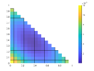
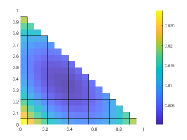
Figure 2: Distribution of the average symmetric epipolar error as a function of barycentric coordinates of the point in the second image w.r.t. the mean point of three points in the first image, for synthetic data (left) and real data (right).

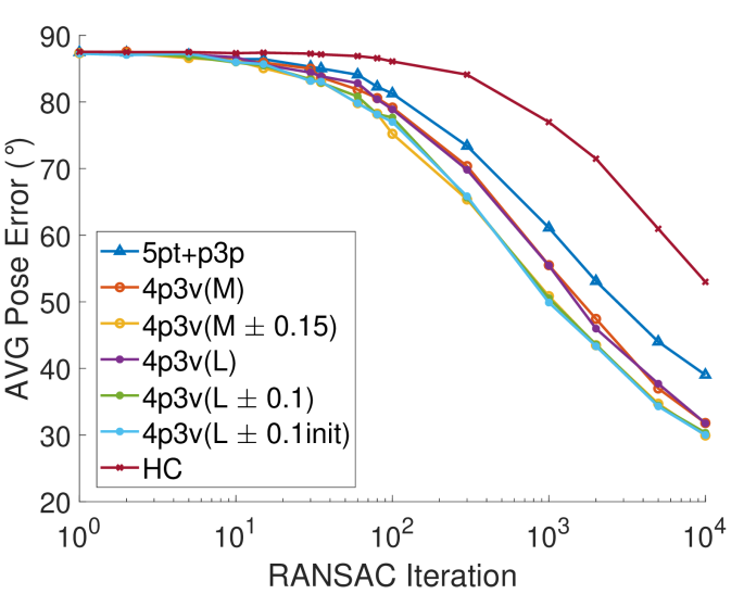
(a) 0.1 Inlier Ratio

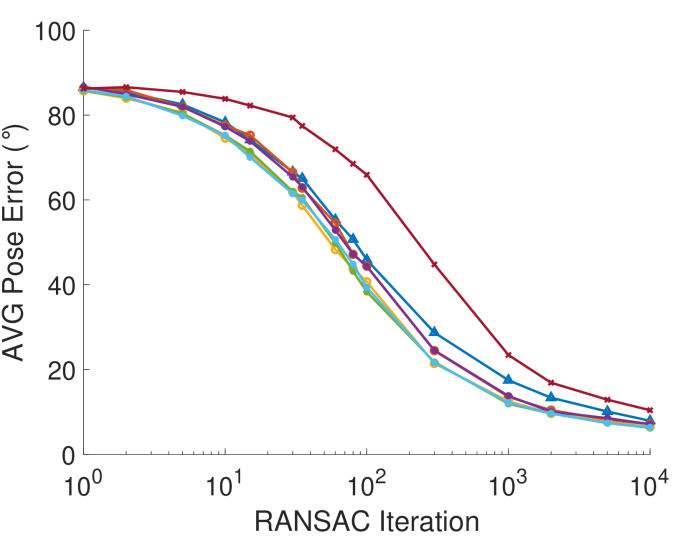
(b) 0.2 Inlier Ratio

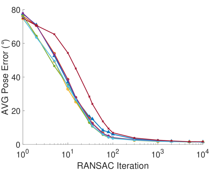
(c) 0.4 Inlier Ratio

Figure 3: Outlier Experiments: We tested the performance, in terms of average pose error (maximum of rotation and translation errors) of the solvers for different inlier ratios and for different numbers of RANSAC iterations. The result is for the Sacre Coeur scene from Phototourism dataset [54]. We plot the results for (a) 0.1 inlier ratio, (b) 0.2 inlier ration and (c) 0.4 inlier ratio.

We performed the same experiment on real data. In this experiment we used the SfM model of the Shop Facade scene from the Cambridge Landmark dataset [23] to obtain image pairs. We extracted 4,525 pairs and used exact projections of 3D points into these pairs to simulate noise-less data. In each pair, we sampled 100 different triplets of points and for each, we performed the same experiment as described above. Altogether, we evaluated 452,500 triplets (corresponding triangles). Fig. 2 (right) again shows the average symmetric epipolar error as a function of barycentric coordinates of the point in the second image. The distribution of errors was very similar to the synthetic data with the minimum at $(0.333,0.333)$, i.e., the mean point.

Noise experiments.  We tested the performance of our solvers, and the state-of-the-art algorithms w.r.t. increasing image noise. We use the SfM model of the botanical garden scene from the ETH3D dataset [53] to obtain instances of points in three views. Perfect correspondences with no noise are generated by projecting the 3D points into the images. We then add increasing amounts of normally distributed noise to these correspondences. Due to the space restrictions, the results of this experiment are presented in the supp. material.

Here we just summarize the main observations from this experiment: Due to the approximate nature of virtual correspondences, our novel solvers return non-zero errors for zero noise. However, at noise levels $\geq 2px$, these solvers return comparable or even better results than the 5pt+P3P/6pt+P3P solvers. This shows that our predicted virtual correspondences are good approximations of real correspondences. The recent state-of-the-art solver [21] is failing in about 50% of the instances for noiseless data, even though the solver was trained on the ETH3D dataset. Thus, the median errors are significantly larger than the median errors of the remaining solvers.

Oracle 4v3p solvers.  To obtain upper bounds for the precision that can be achieved by our proposed solvers, as well as the state-of-the art 4p3v(N) solver [39], we consider the following “oracle” solvers for real experiments: 1) The 4p3v(O)/4p3vf(O) solvers use a correct correspondence(s), i.e., correspondences that satisfies the epipolar constraint for the ground truth relative pose of the first two cameras, as the $5^{\text{th}}$/$6^{\text{th}}$ virtual correspondence between these cameras. Then the 5pt+P3P/6pt+P3P solver is applied to estimate the relative pose of three cameras. The 4p3v(O)/4p3vf(O) shows the maximum precision that our solvers can reach, if they would have been able to predict or infer a precise $5^{\text{th}}$/$6^{\text{th}}$ correspondence from the coordinates of four input correspondences. 2) We test an oracle version of the 4p3v(N) solver. In this 4p3v(NO) solver, instead of performing a one-dimensional search over the $10^{\text{th}}$ degree curve of possible epipoles, we provide the solver with the ground truth epipole. More details on this solver are in the supp. material.

	Sacre Coeur (5000 image triplets)						St. Peters’ Square (5000 image triplets)
Estimator	AVG (∘) $\downarrow$	MED (∘) $\downarrow$	AUC@5∘ $\uparrow$	@10∘	@20∘	Time (s)	AVG (∘) $\downarrow$	MED (∘) $\downarrow$	AUC@5∘ $\uparrow$	@10∘	@20∘	Time (s)	Time ($\mu$s)
cons. 5pt	14.24	15.06	35.20	45.82	56.76	10.15	16.46	19.12	16.49	30.27	46.39	10.04	1113.38
joint 5pt	24.88	14.33	38.45	47.32	55.25	10.29	26.36	10.47	15.31	28.15	43.38	10.36	1113.38
5pt+P3P	23.80	11.86	47.69	55.13	61.25	13.32	26.02	18.67	20.85	33.69	47.17	13.13	1177.90
4p3v(HC) [21]	24.72	13.04	42.81	50.61	57.27	12.60	27.06	19.73	19.78	32.03	45.10	12.22	1*66.06
4p3v(M)	24.77	13.08	42.62	50.58	57.52	13.12	27.44	19.88	18.59	30.99	44.61	12.74	1183.92
4p3v(M $\pm$ 0.15)	24.49	12.42	44.51	52.27	58.91	13.10	25.96	18.92	19.62	32.53	46.24	12.76	1218.71
4p3v(L)	24.92	12.97	42.84	50.71	57.51	13.82	26.78	19.49	18.73	31.51	45.14	12.93	1450.26
4p3v(L $\pm$ 0.1)	24.36	12.35	44.89	52.48	59.00	13.76	26.12	19.06	19.77	32.52	46.06	13.39	1511.28
4p3v(L $\pm$ 0.1 init)	23.95	12.46	44.83	52.78	59.29	15.10	26.09	18.83	19.67	32.68	46.48	14.67	1130.31
4p3v(O)	21.91	11.54	50.18	57.68	63.62	12.85	24.91	16.45	25.67	39.04	51.80	13.11	1180.47
4p3v(NO)	23.34	12.13	46.15	54.54	61.08	10.22	25.89	17.90	21.23	34.79	48.34	10.20	1*73.65

Table 1: The average and median pose errors in degrees, and Area Under the Recall curve (AUC) thresholded at 5^∘, 10^∘ and 20^∘ and the average run-time of RANSAC (in seconds) on a total of 10k image triplets from two scenes of the PhotoTourism dataset [22]. The best results among the solvers for the 4p3v problem (excluding oracle solvers) are marked in bold, the second best are underlined. The last column contains the average running times of particular solvers in $\mu$s over 1,000 trials. ^∗ The time for 4p3v(HC) does not account for its high failure rate, the effective time is usually more than $4\times$ higher [21]. Our time for the 4p3v(HC) is higher than the average time reported in [21]. This can be due to different instances and hardware, and that time in [21] did not involve, e.g., pose extraction from estimated depths. The time for 4p3v(NO) is the time to evaluate one search point. Usually 40 – 1,000 search points have to be evaluated.

Timings.  We computed the average processing times of the solvers over 1,000 random problem instances. The solvers were implemented in C++ within the GC-RANSAC [4] framework using the Eigen library for performing matrix operations. We used the 5pt [38], 6pt [19] and P3P [43] methods implemented in GC-RANSAC for composing the discussed solvers. For 4p3v(HC) we used the implementation from the authors with default settings [21]. The experiments were performed on an Intel(R) Core(TM) i9-10900X CPU @ 3.70GHz. The results for calibrated solvers are reported in the last column of Tab. 1. The discussion of these results is included in Tab. 1 and in Sec. 5. Timings for solvers for partially calibrated cameras are in the supp. mat.

Outlier experiments.  The advantage of 4p3v/4p3vf solvers for the $(4_{4},4_{4},4_{4})$ configuration over the 5pt+P3P and 6pt+P3P solvers for the $(5_{3},5_{3},3_{3})$/$(6_{3},6_{3},3_{3})$ configuration should be visible, especially in the presence of higher outlier contamination and a limited running time for RANSAC. To study this scenario, we evaluate the performance of all proposed solvers, the state-of-the-art 4p3v(HC) solver [21], and the 5pt+P3P/6pt+P3P solvers w.r.t. decreasing inlier ratio, while reporting errors and metrics on different number of RANSAC iterations. For calibrated case we use the Sacre Coeur and St. Peters’ Square scenes from PhotoTourism dataset [54]. We run the solvers inside RANSAC [4] and measure their performance on a series of iterations, only on triplets of images with a given inlier ratio. We used the uniform sampler inside RANSAC. To obtain triplets of images with the given inlier ratio, for each triplet, we keep a certain amount of inliers depending on the total number of correspondences, and replace the rest by uniformly random outlier w.r.t. ground truth poses, correspondences. We filter out image triplets that do not contain enough inliers. The results of this experiment for calibrated cameras and inlier ratios $\{0.1,0.2,0.4\}$ are presented in Figure 3. The results indicate that the new proposed 4p3v solvers reach lower errors faster than the 5pt+P3P solver that samples one more point in the first two cameras. The HC [21] solver, due to its high failure rate, converges even slower than the 5pt+P3P solver.

Real data experiments.  We tested the solvers on two scenes from the validation set of the IMC2020 benchmark [22]. The scenes, Sacre Coeur and St. Peter’s Square, come from the PhotoTourism dataset [54] and provide ground truth pose via a COLMAP [52] reconstruction. To form image triplets, we iterated through the point correspondences provided in [22] and selected pairs of image pairs that share one view. Since the provided correspondences do not contain descriptors, we detected RootSIFT [35, 2] features in all three images of each triplet. We then matched features between the view pairs 1-2 and 1-3 by standard nearest neighbors matching. To enforce cycle consistency, we kept only those correspondences that were matched to the same features in all view pair combinations. In total, we collected 5,000 image triplets from each scene.

To estimate the relative poses between the images of each triplet, we apply the Graph-Cut RANSAC [4] robust estimator. The point-to-model residual function is chosen to be the Sampson error of a triplet correspondence average over image pairs 1-2 and 1-3. We calculate the error of the triplet pose by, first, taking the average of the relative rotation and translation errors coming from essential matrices $\textbf{E}_{12}$ and $\textbf{E}_{13}$ given the ground truth relative pose. Finally, we take the maximum of the averaged rotation and translation errors (both measured in degrees) as the pose error [22].

We test the focal length solvers on the KITTI dataset [17]. We form triplets by connecting the stereo pair from the $i$-th frame to the left image in the $i+1$-th one. Similarly as before, we extract and match RootSIFT features.

Tab. 1 and 2 report the average and median pose error in degrees, the Area Under the recall Curve (AUC) thresholded at $5^{\circ}$, $10^{\circ}$, and $20^{\circ}$, and the average processing time in seconds. The results are discussed in Sec. 5. More results on real data are in the supp. material.

5 Discussion and limitations

In this paper, we present solvers to the challenging problems of estimating the relative pose of three calibrated and partially calibrated cameras from four correspondences. We tested our solvers on different real-world datasets (Tabs. 1 and 2) from which several conclusions can be drawn:

• The very simple 4p3v(M$\pm\delta$)/4p3vf(M$\pm\delta$) solvers, which use only mean points as virtual “approximate” correspondences and two more points in their vicinity, achieve state-of-the-art results on the challenging 4p3v/4p3vf problems. Compared to state-of-the-art solvers for the 4p3v problem, our new 4p3v(M$\pm\delta$)/4p3vf(M$\pm\delta$) solvers are extremely simple to implement since they just run existing well-known 5pt/6pt and P3P solvers that are available in many libraries. They do not require any network training, parameter tuning, optimization, or implementation of complex solution techniques as required by the 4p3v(HC) and 4p3v(N) solvers. As such, our novel M-solvers should be considered as new baselines for the 4p3v/4p3vf problems.

• The 4p3v(M$\pm\delta$)/4p3vf(M$\pm\delta$) solvers call the 5pt/6pt solvers three times and are thus slower than the 4p3v(M)/4p3vf(M) solvers. However, since $\delta$-solvers provide better estimates, the total running times of RANSAC with the 4p3v(M$\pm\delta$)/4p3vf(M$\pm\delta$) solvers are almost identical to the running times of RANSAC with the 4p3v(M)/4p3vf(M) solvers, and comparable to the 4p3v(HC) [21], while achieving better precision.

• Our novel L-based solvers for the 4p3v problem show a slight improvement over the M-based solvers (cf. Tab 1). Although the architecture of our proposed network is very simple and can be considered more as a prototype, it shows the potential to learn virtual correspondences and achieve results closer to the oracle 4p3v(O) solver.

• For the 4p3vf problem with unknown focal length, the proposed 4p3vf(M$\pm\delta$) solver achieves results very close to the oracle 4p3vf(O) solver (cf. Tab. 2). For this problem, the 4p3vf(L) solver achieves smaller average but larger median errors than the 4p3vf(M) solver. We attribute this to the fact that we use a network trained for the 5pt solver, while the 6pt solver exhibits more degenerate configurations, and the fact that for this dataset, mean point correspondences are most likely very good approximations of correct correspondences.

• The state-of-the-art results of our solvers show the potential of the proposed method based on virtual correspondences to be applied to other camera geometry problems. A discussion on this can be found in the supp. material.

• We are the first to properly compare solvers for two different minimal configurations, i.e., the $(5_{3},5_{3},5_{3})$ and $(4_{4},4_{4},4_{4})$ for three calibrated cameras on real-world datasets within a state-of-the-art RANSAC framework [4]. Although our novel solvers achieve state-of-the-art results for the $(4_{4},4_{4},4_{4})$ configuration, our results show that in scenarios where we have enough computational time and a small outlier contamination, it is preferable to use the solver 5pt+P3P and sample one more point in two views. However, the results of the oracle 4p3v(O) solver suggest that there is still room for improving 4p3v solvers. Moreover, our outlier experiments (cf. Fig 3) show that in the presence of larger outlier ratios and limited computational time, the proposed 4p3v solvers are preferable.

Estimator	AVG (∘) $\downarrow$	MED (∘) $\downarrow$	AUC@1∘ $\uparrow$	@2.5∘	@5∘	@10∘	Time (s)
cons. 6pt	11.69	11.14	11.77	47.34	70.30	84.57	10.05
joint 6pt	11.59	11.09	12.85	48.77	71.05	85.00	10.05
6pt+p3p	11.83	11.00	15.79	51.14	71.73	84.89	10.11
4p3vf(M)	11.89	11.05	14.47	49.64	70.81	84.44	10.07
4p3vf(M $\pm$ 0.15)	11.66	10.99	15.74	51.36	72.05	85.27	10.07
4p3vf(L)	11.58	11.10	12.88	48.79	71.09	85.06	10.07
4p3vf(L $\pm$ 0.1)	11.69	11.01	15.44	50.68	71.55	85.07	10.10
4p3vf(L $\pm$ 0.1 init)	11.74	11.01	15.30	50.30	71.34	84.84	10.18
4p3vf(O)	11.58	10.98	16.05	51.59	72.25	85.51	10.09

Table 2: Results on KITTI dataset [17] for partially calibrated cameras. The reported statistics are the same as in Tab. 1.

6 Conclusion

In this paper, we consider the highly challenging problem of relative pose estimation of three calibrated and partially calibrated cameras from four correspondences. We propose a novel framework that solves these problems using existing efficient solvers by simply predicting a $5^{\text{th}}$/$6^{\text{th}}$ point correspondence(s). We propose several solvers based on this framework, one simply using mean coordinates of input points (M-based solvers) and one using a trained predictor (L-based solvers). Extensive experiments show that our solvers achieve state-of-the-art performance on real data for the configuration of four points in three views. At the same time, our M-based solvers are trivial to implement, especially compared to the current state-of-the-art [21].

Acknowledgements.  Charalambos Tzamos was supported by the Czech Science Foundation (GAČR) JUNIOR STAR Grant (No. 22-23183M) and by SGS project (No. SGS23/173/OHK3/3T/13). Daniel Barath was supported by the ETH postdoc fellowship. Torsten Sattler was supported by the EU Horizon 2020 project RICAIP (grant agreement No. 857306) and the European Regional Development Fund under project IMPACT (No. CZ.02.1.01/0.0/0.0/15_003/0000468). Zuzana Kukelova was supported by the Czech Science Foundation (GAČR) JUNIOR STAR Grant (No. 22-23183M).

Supplementary Material

This supplementary material provides more details on the architecture, training data, and training of the network used in the 4p3v(L)/4p3vf(L) solvers presented in Sec. 3.1 and 3.2 of the main paper (Sec. 7), a discussion of the proposed method for solving camera geometry problems using virtual correspondences (Sec. 8), more details on the experiments presented in Sec. 4 of the main paper (Sec. 9), and potential directions for future work (Sec. 10).

7 Details on the network

As described in the main paper, we use a simple MLP based backbone, similar to [10]. More precisely, our input consists of four 6-vectors, of the $x,$ and $y$ coordinates of four point correspondences in three views. The first part of the model is a shared MLP 3-block of dimensions 6, 32, and 32, exporting a 32-dimensional feature for every correspondence. Then we apply a channel-wise max pooling aggregation, which is the concatenated at the end of each 32-dimensional feature. This results in having an 64-vector for each correspondence, which are passed into another shared MLP 3-block of 64, 64, and 64 dimensions. We aggregate those vector via a max pooling function to get a 64-vector encoding, which eventually passes through an MLP 3-block to reduce the dimension gradually from 64, to 32 and finally to 2, which will be the prediction of the $x$ and $y$ coordinates in the second camera. In all MLPs, in the first 2 layers of the blocks, we use a Leaky RELU activation function [62] with slope 0.01. As for the last layer of the MLPs, in the first two blocks, we use a RELU activation function, while in the last MLP we use a $\tanh$ activation, since we want the output to be in the range $(-1,1)$. For a visualization of the architecture, see Figure 5.

For both training and validation, we use synthetic data. Our synthetic dataset contains 1M input instances. 70% of the dataset is used for training while the rest 30% is used for validating the performance of the network. We generate 10K 3D points inside a 10$\times$10$\times$10 cube, and to generate each instance, we pick 4 random points and project them to 3 cameras with random rotations and translations that view the cube from a random distance between 20 to 50 units.

The network is implemented in PyTorch [41], and we use the Adam optimizer [25] for the training. We train it in batches of 1024 input instances, with a fixed learning rate of 1e-5. In our experiments, the network converges in about 30 epochs.

8 Solving camera geometry problems using virtual correspondences

The proposed methods generating virtual correspondences, i.e., the learning-based and the mean-point-based methods that were used in the novel solvers for the 4p3v and 4p3vf problems, can be, in general, applied to other camera geometry estimation problems.

M-based solvers  While the mean point correspondence used in the M-based solvers can provide a good approximation of a correct correspondence, such a correspondence can be noisy. Note that all state-of-the-art 4p3v solvers (including 4p3v(HC) and 4p3v(N)) rely on certain approximations without establishing theoretical proofs to quantify their accuracy. In contrast, the error of our virtual correspondence is bounded: As mentioned in the main paper, it can be proven that the error of the virtual correspondence $\mathbf{m}^{1}\leftrightarrow\mathbf{m}^{2}$ is bounded by the maximum distance of the mean point $\mathbf{m}^{2}$ from the vertices of the triangle $\left\{\mathbf{x}_{i}^{2},\mathbf{x}_{j}^{2},\mathbf{x}_{k}^{2}\right\}$. Here we provide a simple proof.

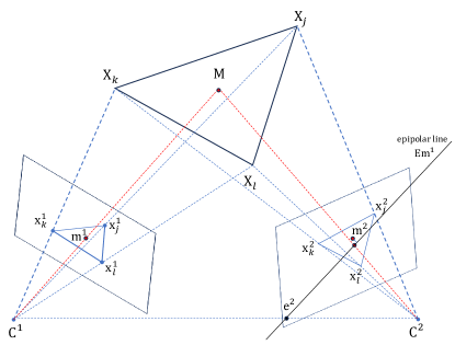
Figure 4: Illustration of the considered situation.

Lemma 1.

Let us assume two cameras with camera centers $\mathbf{C}^{1}$ and $\mathbf{C}^{2}$ that observe 3D points $X_{i},X_{j},$ and $X_{k}$. Let $\left\{\mathbf{x}_{i}^{1},\mathbf{x}_{j}^{1},\mathbf{x}_{k}^{1}\right\}$ and $\left\{\mathbf{x}_{i}^{2},\mathbf{x}_{j}^{2},\mathbf{x}_{k}^{2}\right\}$ be the projections of these 3D points in camera 1 and camera 2, respectively. Let $\mathbf{m}^{1}$ be the mean point of the points $\left\{\mathbf{x}_{i}^{1},\mathbf{x}_{j}^{1},\mathbf{x}_{k}^{1}\right\}$ and let $\mathbf{E}$ be the essential matrix between these two cameras, i.e., a matrix that satisfies $\mathbf{x}_{l}^{2^{\top}}\mathbf{E}\mathbf{x}_{l}^{1}=0,\;\forall l\in\left\{i,j,k\right\}$. Then the epipolar line $\mathbf{E}\mathbf{m}^{1}$ passes through the triangle $\left\{\mathbf{x}_{i}^{2},\mathbf{x}_{j}^{2},\mathbf{x}_{k}^{2}\right\}$.

Proof.

The camera center $\mathbf{C}^{1}$ and the 3D points $\mathbf{X}_{i},\mathbf{X}_{j},$ and $\mathbf{X}_{k}$ form a tetrahedron $T^{1}$ (see Figure 4.). The projections $\left\{\mathbf{x}_{i}^{1},\mathbf{x}_{j}^{1},\mathbf{x}_{k}^{1}\right\}$ in the first camera lie at the edges of this tetrahedron $T^{1}$. The ray from the camera center $\mathbf{C}^{1}$ through the mean point $\mathbf{m}^{1}$ thus lies inside the tetrahedron $T^{1}$ and intersects the plane defined by 3D points $\mathbf{X}_{i},\mathbf{X}_{j},$ and $\mathbf{X}_{k}$ in a point $\mathbf{M}$ that lies inside the triangle defined by $\left\{\mathbf{X}_{i},\mathbf{X}_{j},\mathbf{X}_{k}\right\}$.

The camera center $\mathbf{C}^{2}$ and the 3D points $\mathbf{X}_{i},\mathbf{X}_{j},$ and $\mathbf{X}_{k}$ form a tetrahedron $T^{2}$. Again, the projections $\left\{\mathbf{x}_{i}^{2},\mathbf{x}_{j}^{2},\mathbf{x}_{k}^{2}\right\}$ lie at the edges of the tetrahedron $T^{2}$. The ray passing through the camera center $\mathbf{C}^{2}$ and the 3D point $\mathbf{M}$ lies inside the tetrahedron $T^{2}$ and thus intersects the image plane of the second camera at a point that lies inside the triangle defined by the points $\left\{\mathbf{x}_{i}^{2},\mathbf{x}_{j}^{2},\mathbf{x}_{k}^{2}\right\}$. By construction, the projection of $\mathbf{M}$ into the second camera lies on the epipolar line $\mathbf{E}\mathbf{m}^{1}$. Therefore, the epipolar line $\mathbf{E}\mathbf{m}^{1}$ which is a line connecting this point and the epipole $\mathbf{e}^{2}$, passes through the triangle $\left\{\mathbf{x}_{i}^{2},\mathbf{x}_{j}^{2},\mathbf{x}_{k}^{2}\right\}$. ∎

Obviously, it follows from Lemma 1 that since the epipolar line $\mathbf{E}\mathbf{m}^{1}$ passes through the triangle $\left\{\mathbf{x}_{i}^{2},\mathbf{x}_{j}^{2},\mathbf{x}_{k}^{2}\right\}$, the maximum distance of the mean point $\mathbf{m}^{2}$ to the epipolar line $\mathbf{E}\mathbf{m}^{1}$ is equal to the maximum distance of $\mathbf{m}^{2}$ to the vertices of the triangle.

The final error of the estimated pose, however, depends on many aspects, e.g., the baseline and the view angles of the cameras w.r.t. the 3 points used, the depth of these points, and the size of the triangle. Although in theory, this error could be large, our experiments show that it does not lead to significantly larger errors than the 5pt+P3P method, which samples an additional fifth correspondence, rather than predicting or approximating one (e.g., for the ShopFacade from the Cambridge Landmarks dataset, avg/med epipolar error of the mean point prediction is 6.01px/2.94px).

A deeper analysis of the error propagation for virtual correspondences is out of the scope of this paper and better fits a follow-up publication dealing with the proposed method as a general method for solving camera geometry problems. In this paper, we decided to focus on two important problems of estimating the relative pose of three cameras from four point correspondences, which have been considered as not fully solved for decades.

L-based and $\delta$-based solvers  Our simple L-based and $\delta$-based solvers, that either predict “a shift” of the mean point in the second image using a simple network or generate two more potential correspondences in the $\delta$-vicinity of the mean-point correspondence, show the potential to deal with noise in the mean-point correspondences. Note that we tested only a simple network architecture and a simple strategy to generate point correspondences in the $\delta$-vicinity of the mean-point correspondence. More advanced network architectures (e.g., using a set transformer architecture [32]) or a more advanced method to generate additional $\delta$-point correspondences have the potential to improve the results even more and reduce the gap between our proposed 4p3v/4p3vf solvers and the oracle 4p3v(O)/4p3vf(O) solvers.

Figure 5: The architecture of our network. With LR we denote the Leaky RELU activation function [62]. The input consists of four 6-vectors, one for each correspondence. Each 6-vector contains the $x$ and $y$ coordinates of a correspondence in three views. First, the input passes through a shared MLP block, so that each 6-vector is processed independently. Then, the output feature vectors of dimension 32 are aggregated using a channel-wise max pooling function, and the result of it is concatenated at the end of each feature vector. Then, there is one more block of shared MLPs, of which the results are aggregated again by a max pooling, to get a single 64-vector. We reduce the dimensions of this vector by passing it through an MLP block, of which the last layer has 2 nodes and a $\tanh$ activation function.

Use-cases for virtual correspondences  We believe that the proposed method based on virtual correspondences is general and, due to its simplicity, has the potential to generate efficient and easy-to-implement solvers for other problems. Generating one or potentially more virtual correspondences using only the locations of the input correspondences can allow to solve complex minimal problems using much simpler non-minimal solvers, while still sampling only a minimal number of points inside RANSAC.

In the first step, our M-based solvers solve 5pt/6pt relative pose problems of two calibrated/partially calibrated cameras using only a sub-minimal sample of four point correspondences. The good performance of these solvers, not only for the pose of the whole triplet of cameras but also for the relative pose of the first two cameras (cf. Sec. 9.2 and Figure 7), suggests that the method based on virtual correspondences can also be used to solve minimal problems using sub-minimal samples inside RANSAC in some scenarios.

To better illustrate this use-case, in Sec. 9.6 we show preliminary results for the well-known 5pt relative pose problem, where we sample only four point correspondences inside RANSAC and generate the $5^{\text{th}}$ correspondence as the mean point (or points in its $\delta$-vicinity) of three corresponding points in both images. Even though four points in two views define an infinite number of camera poses that can observe these points, we show that, in practice, such a mean-point correspondence is usually a quite good approximation of a correct correspondence. While this $5^{\text{th}}$ correspondence can be noisy, the resulting 4pt(M) and 4pt(M$\pm\delta$) solvers show comparable performance to the 5pt solver inside RANSAC. This shows the potential for applying such a sub-minimal solver in scenarios with lots of outliers and noisy data, where sampling one less point may show some improvement.

While the method based on virtual correspondences can be theoretically applied to any camera geometry problem, we see larger promise in relative pose problems, where it is sufficient to find one 2D point that is sufficiently close to the epipolar line. For absolute pose solvers, a virtual correspondence will need to be close to a 2D point instead of an epipolar line.

9 Experiments

This section provides more details on the experiments presented in Sec. 4 of the main paper, as well as results showing the potential of the proposed method based on virtual correspondences to solve minimal problems using sub-minimal samples of points.

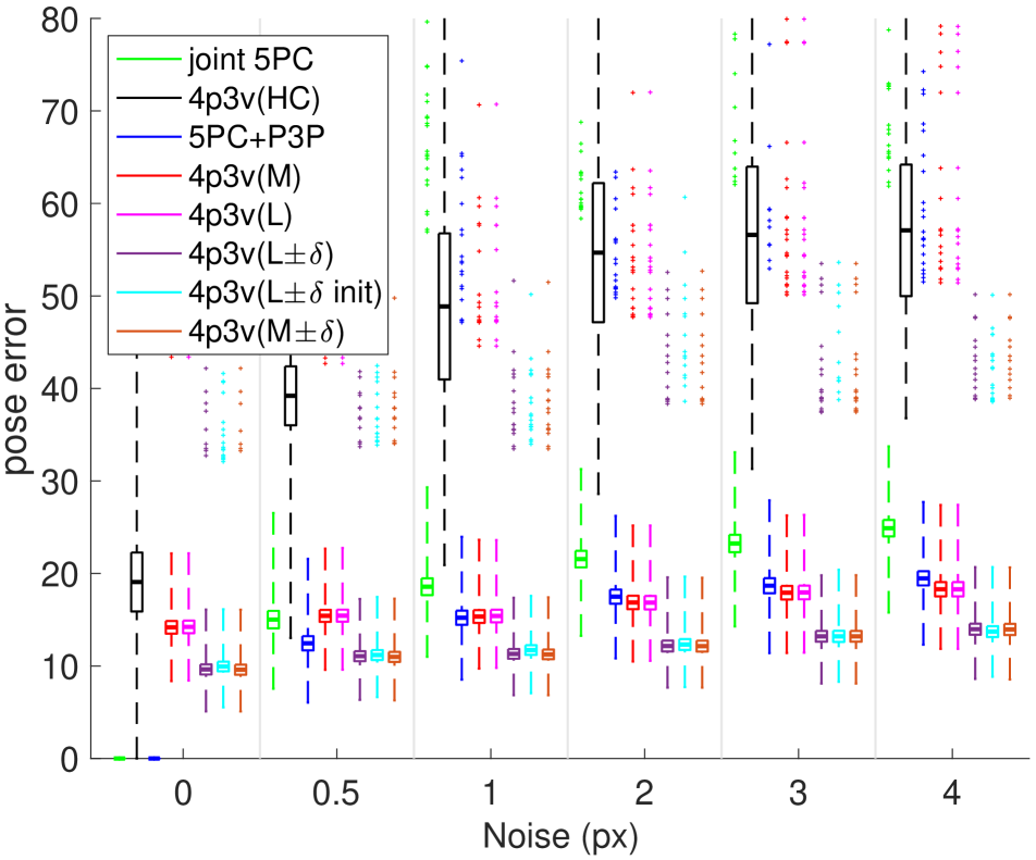
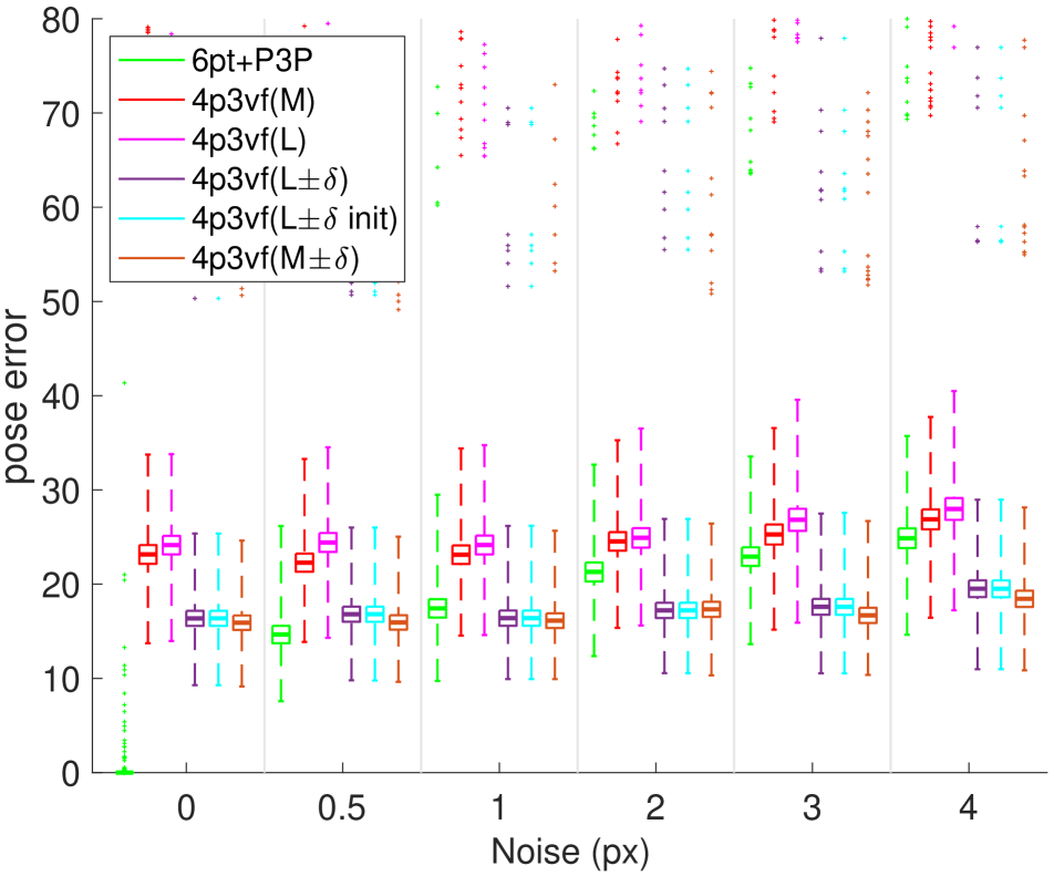
Figure 6: Noise experiment showing the pose error measured as $\texttt{max}(\texttt{avg}(e(\mathtt{R}_{12}),e(\mathtt{R}_{13})),\texttt{avg}(e(\mathtt{t}_{12}),e(\mathtt{t}_{13})))$, for the calibrated 4p3v problem (left) and the partial calibrated 4p3vf problem (right) as a function of the noise scale in pixels. Here, $\mathtt{R}_{ij}$ and $\mathtt{t}_{ij}$ are the relative rotation and translation of the $i^{\text{th}}$ and $j^{\text{th}}$ views, respectively.

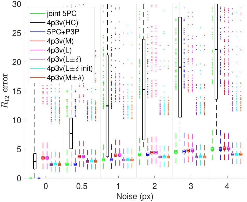
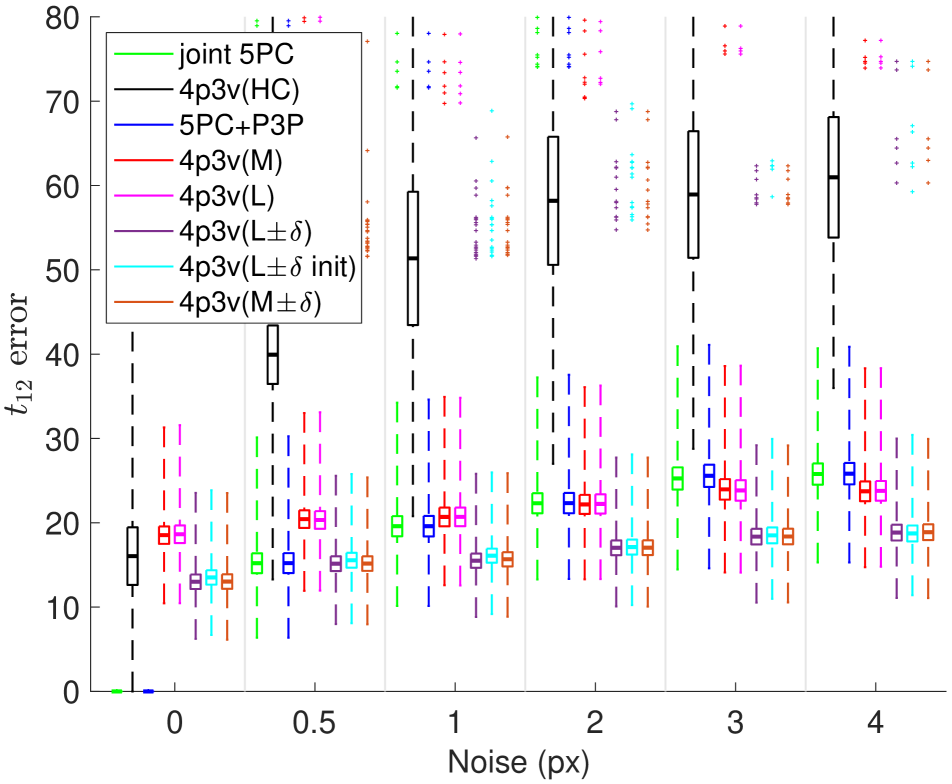
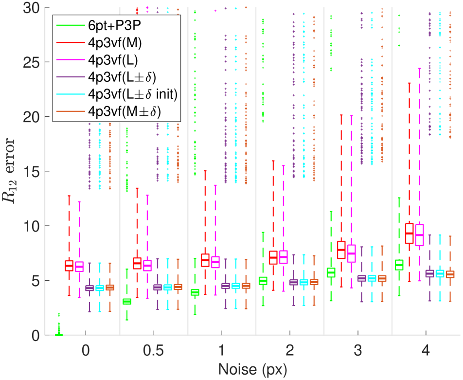
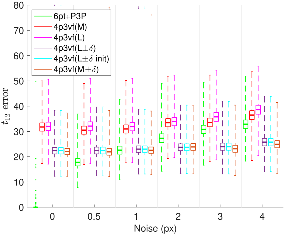
Figure 7: Noise experiment showing $e(\mathtt{R}_{12})$ (left) and $e(\mathtt{t}_{12})$ (right) as functions of the noise scale in pixels for the calibrated 4p3v problem (top) and the partially calibrated 4p3vf problem (bottom). Here $\mathtt{R}_{12}$ and $\mathtt{t}_{12}$ are the relative rotation and translation between the first two views.

9.1 Oracle solvers

We first provide more details on implementation of our oracle version of the 4p3v(N) solver [39], i.e. the 4p3v(NO) solver.

In the 4p3v(NO) solver, instead of performing an one-dimensional search over the $10^{\text{th}}$ degree curve of possible epipoles, we provide the solver with the ground truth epipole. To simulate the effect of sampling four points for this solver inside RANSAC, instead of using the second epipole and the epipolar line homography to get the essential matrix $\mathtt{E}$, as suggested in the implementation details of [39], we use the second suggested way on how to obtain $\mathtt{E}$, i.e., using their 3pt+ep solver. However, we feed the 3pt+ep solver with four points and use SVD instead of the null space. The rest of the solver performs the triangulation and registers the last camera using the P3P solver [43]. This is identical to the original 4p3v(N) solver. However, in this case we do not need to use the fourth point correspondence to select the pose that minimizes the reprojection error. Similarly, we do not need to use refinement. Remember that the original 4p3v(N) solver needs to call these evaluations for each search step on the $10^{\text{th}}$ degree curve of possible epipoles (usually $40{\times}-1000{\times}$ [39]). Moreover, this solver has several sources of errors, e.g., the $10^{\text{th}}$ degree curve is affected by noise; sparse sampling of the points on the curve introduces additional potentially large noise in the epipole; the reprojections of the fourth image point in the third view, traced out by sweeping through the curve of possible epipoles, generates complex curves in the third view, with the reprojection cost function having a lot of local minima. In the paper [39] it was reported that even for exact data and 1000 search points followed by refinement at multiple local minima the failure rate of the solver is $\approx 3\%$. Therefore, we expect the original solver 4p3v(N) to perform much worse that the “oracle” 4p3v(NO) solver used in the experiments presented in the main paper.

9.2 Noise experiments

We tested the performance of our solvers and the state-of-the-art algorithms w.r.t. increasing image noise. We used the SfM model of the botanical garden scene (randomly selected from all scenes) from the ETH3D dataset [53] to obtain instances of 5/6 points in three views by identifying images in the scene that share 3D points. Perfect noise-free correspondences are generated by projecting the 3D points into the images. We then add increasing amounts of normally distributed noise to these correspondences. We generated more than 9k instances, but show only 1k results per plot to avoid clutter. Note that the 4p3v(HC) solver was trained on the ETH3D dataset while our L-based solvers were trained on purely synthetic data.

The results for increasing noise in the image points are shown in Figs. 6 and 7. The results are represented by boxplot function which shows the 25% to 75% quantiles as a box with a horizontal line at median. Crosses show data beyond 1.5 times the interquartile range. Let $e(\mathtt{R}_{ij})$ be the error of the estimated relative rotation between cameras $i$ and $j$, computed as the angle in the axis-angle representation of $\mathtt{R}_{ij}^{-1}\mathtt{R}_{ij}^{\mathtt{GT}}$ and let $e(\mathtt{t}_{ij})$ be the error of the estimated translation computed as the angle between the two unit vectors corresponding to the translations. Fig. 6 shows boxplots of pose errors measured in the same way as in our experiments in the main paper (cf. Sec. 4 in the main paper), i.e. as $\texttt{max}(\texttt{avg}(e(\mathtt{R}_{12}),e(\mathtt{R}_{13})),\texttt{avg}(e(\mathtt{t}_{12}),e(\mathtt{t}_{13})))$, for the calibrated 4p3v problem (left), and the partially calibrated 4p3vf problem (right). The errors are zoomed into an interesting interval and are shown as functions of varying noise from $0px$ to $4px$.

Due to the approximate nature of the virtual correspondences, our newly proposed M-based and L-based solvers return non-zero errors for zero noise. However, at noise levels $\geq 1px$, our $\delta$-based solvers (both M and L), and for the calibrated case even the pure 4p3v(M) and 4p3v(L) solvers, return comparable or even better results than the 5pt+P3P and 6pt+P3P solvers. Note that the 5pt+P3P and 6pt+P3P solvers sample one/two more points (real correspondences) in the first two cameras, and these points are affected only by the considered noise. This shows that our predicted virtual correspondences are good approximations to real correspondences. For the calibrated case, the recent state-of-the-art solver [21] is failing in about 50% of the instances for noiseless data, even though the solver was trained on the ETH3D dataset. Thus, the median errors are significantly larger than the median errors of the remaining solvers.

The rotation and translation errors in the first two views, i.e., $e(\mathtt{R}_{12})$ and $e(\mathtt{t}_{12})$, for both the calibrated (top row), and the partially calibrated case (bottom row) are shown in Fig. 7. For the partially calibrated case, our new solvers generate two approximate virtual correspondences in the first two views. Therefore, the 4p3vf(M) and 4p3vf(L) solvers have slightly larger errors than the 6pt+P3P solver for all considered noise levels. However, similarly to the pose errors in Figure 6, at noise levels $\geq 1px$ our $\delta$-based solvers (both M and L), and for the calibrated case even the pure 4p3v(M) and 4p3v(L) solvers, return comparable or even better results in the first two views than the 5pt [38] and 6pt [59] solvers, here represented by the results of 5pt+P3P and 6pt+P3P solvers. This shows an interesting potential of using our solvers for the two-view relative pose estimation problems by solving these problems from sub-minimal samples.

9.3 Outlier experiments

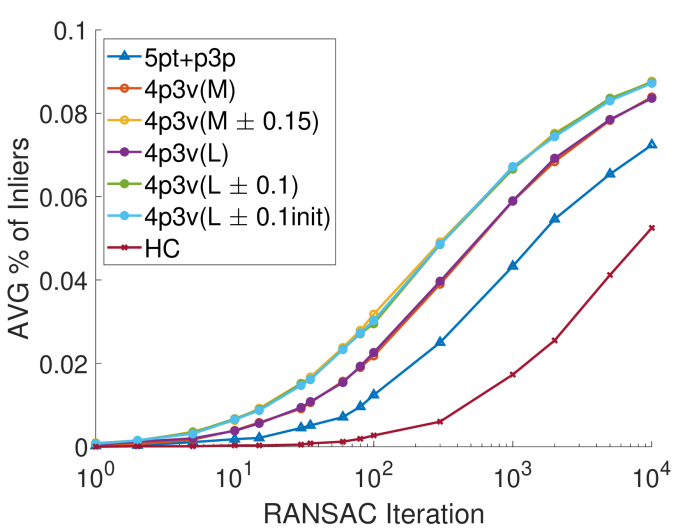
(a) 0.1 Inlier Ratio

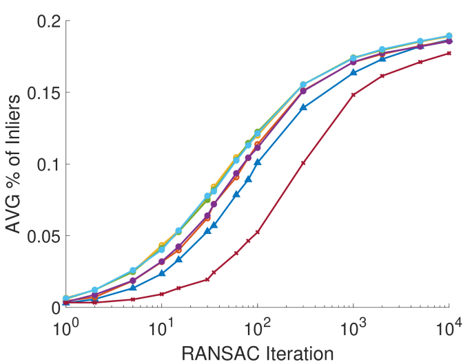
(b) 0.2 Inlier Ratio

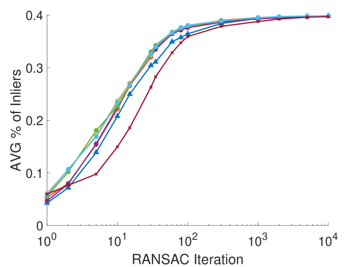
(c) 0.4 Inlier Ratio

Figure 8: Outlier Experiments: We tested the performance, in terms of the average percentage of inliers, of the solvers for different inlier ratios and for different numbers of RANSAC iterations. Results are shown for the Sacre Coeur scene from PhotoTourism dataset [54]. We plot the results for (a) 0.1 inlier ratio, (b) 0.2 inlier ratio, and (c) 0.4 inlier ratio.

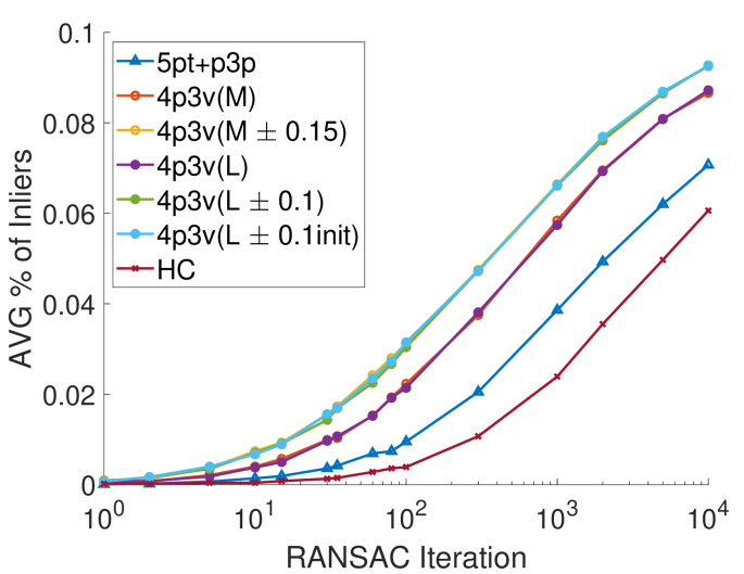
(a) 0.1 Inlier Ratio

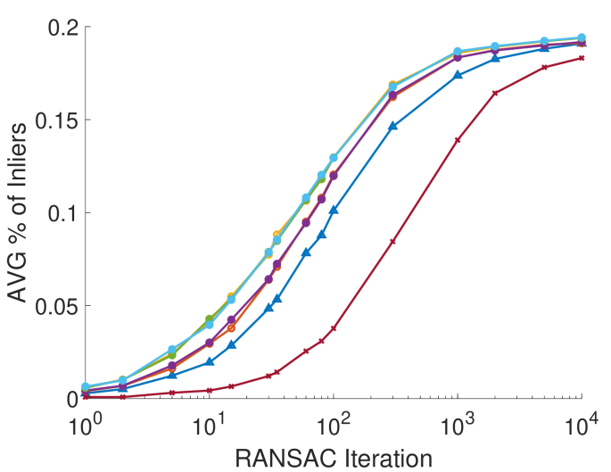
(b) 0.2 Inlier Ratio

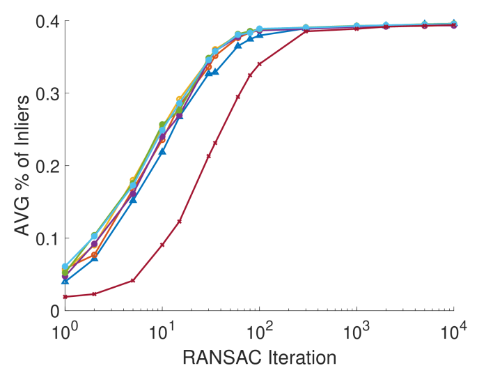
(c) 0.4 Inlier Ratio

Figure 9: Outlier Experiments: We tested the performance, in terms of the average percentage of inliers, of the solvers for different inlier ratios and for different numbers of RANSAC iterations. Results are shown for the St Peters’ Square scene from PhotoTourism dataset [54]. We plot the results for (a) 0.1 inlier ratio, (b) 0.2 inlier ratio, and (c) 0.4 inlier ratio.

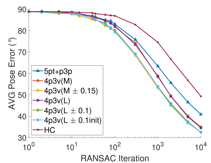
(a) 0.1 Inlier Ratio

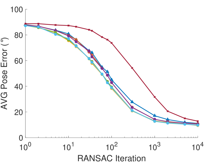
(b) 0.2 Inlier Ratio

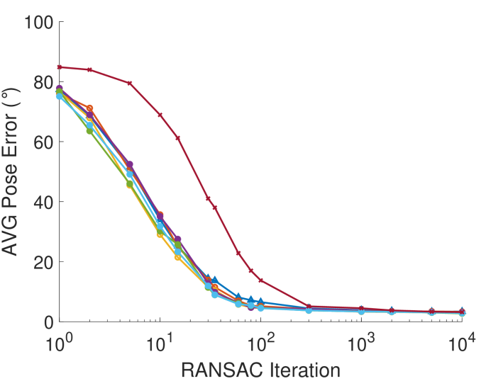
(c) 0.4 Inlier Ratio

Figure 10: Outlier Experiments: We tested the performance, in terms of the average pose error (maximum of rotation and translation errors), of the solvers for different inlier ratios and for different numbers of RANSAC iterations. Results are shown for the St. Peters’ Square scene from the PhotoTourism dataset [54]. We plot the results for (a) 0.1 inlier ratio, (b) 0.2 inlier ratio, and (c) 0.4 inlier ratio.

The outlier experiments are implemented as described in Section 5 the main paper. Here we provide additional plots for inlier ratios $\{0.1,0.2,0.4\}$. In Figures 8 and 9, we show the performance of each solver w.r.t. the percentage of inliers that they gather, on different RANSAC iterations, for the Sacre Coeur and St. Peters’ Square scenes, respectively. In Figure 10, we show the performance of the solvers w.r.t. average pose error on the St. Peters’ Square scene, similar to the one included in the main paper for Sacre Coeur. The pose error was measured in the same way as in our experiments in the main paper (cf. Sec. 4 in the main paper), i.e., as $\texttt{max}(\texttt{avg}(e(\mathtt{R}_{12}),e(\mathtt{R}_{13})),\texttt{avg}(e(\mathtt{t}_{12}),e(\mathtt{t}_{13})))$.

For low inlier ratios and in early RANSAC iterations, we observe that the $\delta$-based solvers perform the best, slightly better than 4p3v(M) and 4p3v(L). 5pt+P3P and 4p3v(HC) solvers show worse performance than our proposed solvers in this experiment. Increasing the inlier ratio up to 0.4, the performance of 5pt+P3P increases, becoming similar to the performance of 4p3v(M) and 4p3v(L). Even for an inlier ratio of 0.4, 4p3v(HC) exhibits a slower convergence due to the higher failure rate.

9.4 Timings

	6pt+P3P	4p3vf(M)	4p3vf(M$\pm\delta$)	4p3vf(L)	4p3vf(L$\pm\delta$)	4p3vf(L$\pm\delta$init)
Time ($\mu$s)	106.67	117.28	295.87	758.59	953.34	2162.77

Table 3: The average run-time, averaged over more than 10k instances of the Sacre Coeur scene of the PhotoTourism dataset [54], of the solvers for the partially calibrated case.

In the main paper, we presented run-times of the proposed solvers as well as the state-of-the-art solvers for the relative pose problem of three calibrated cameras (cf. Table 1 (last column) in the main paper). Here we present run-times of solvers for partially calibrated cameras. To measure the run-times of the solvers, we calculated the average run-time of each solver on more than 10k instances of the Sacre Coeur scene of the PhotoTourism dataset [54]. The run-times are reported in Table 3. The experiments were performed on an Intel(R) Core(TM) i9-10900X CPU @ 3.70GHz. The average run-times of the L-based solvers are higher, because we run the network on the CPU and without batching. In general, the implementations of all proposed solvers are not optimized for speed, and we still see room for speeding them up.

9.5 $\delta$-based solvers

We tested our $\delta$-based solvers for different values of $\delta$ and measured their performance. The results of this experiment for the calibrated 4p3v problem on the Sacre Coeur and St. Peters’ Square scenes from the PhotoTourism dataset [54] are reported in Table 4.

In general, there is no common value of the $\delta$ shift that leads to the best results on all datasets. This is expected since the precision of the mean-point correspondence depends on many different factors, e.g., the viewing angles of the cameras, the type of the motion, the depth and spatial distributions of the 3D points, etc. In general, choices of $\delta$ between $0.05$ and $0.15$ resulted in the best results on the tested datasets. For the 4p3v(L$\pm\delta$), and 4p3v(L$\pm\delta$init) solvers a bit smaller shifts are preferable, since these solvers are already shifting the mean-point correspondence by a prediction returned by the network. On the tested datasets a good trade-off between the precision and the running time of RANSAC is achieved using $\delta=0.15$ for the 4p3v(M$\pm\delta$) solver, and $\delta=0.1$ for the 4p3v(L$\pm\delta$) and 4p3v(L$\pm\delta$init) solvers.

The results for the partially calibrated 4p3vf problem on the KITTI dataset [17] are reported in Table 5. Similar to the calibrated case, similar performance is observed for various choices of $\delta$. However $\delta=0.1$ seems to be the best choice for all three solvers, namely 4p3vf(M$\pm\delta$), 4p3vf(L$\pm\delta$), and 4p3vf(L$\pm\delta$init).

Designing a strategy for selecting a suitable $\delta$, e.g., based on the shape of the triangle used to compute the virtual correspondence or based on results obtained using different $\delta$-shifts in early iterations of RANSAC, or from a few images from the given sequence of images (if we e.g. have to process a sequence of images that undergo a similar motion) would be an interesting future work.

	Sacre Coeur (5000 image triplets)						St. Peters’ Square (5000 image triplets)
Estimator	AVG (∘) $\downarrow$	MED (∘) $\downarrow$	AUC@5∘ $\uparrow$	@10∘	@20∘	Time (s) $\downarrow$	AVG (∘) $\downarrow$	MED (∘) $\downarrow$	AUC@5∘ $\uparrow$	@10∘	@20∘	Time (s) $\downarrow$
4p3v(M $\pm$ 0.05)	24.35	12.39	44.83	52.43	59.07	13.14	26.28	19.01	20.34	32.95	46.52	12.81
4p3v(M $\pm$ 0.1)	24.42	12.63	44.16	51.85	58.53	13.11	26.16	19.07	19.51	32.44	46.00	13.63
4p3v(M $\pm$ 0.15)	24.49	12.42	44.51	52.27	58.91	13.10	25.96	18.92	19.62	32.53	46.24	12.76
4p3v(M $\pm$ 0.2)	24.24	12.58	44.36	52.15	58.76	13.11	26.32	19.20	19.24	32.15	45.92	12.75
4p3v(M $\pm$ 0.25)	23.80	12.63	44.28	52.12	58.81	13.11	26.63	19.30	19.02	31.90	45.64	12.79
4p3v(L $\pm$ 0.05)	24.37	12.43	44.90	52.49	58.94	13.76	26.00	19.10	20.00	32.83	46.53	14.74
4p3v(L $\pm$ 0.075)	24.32	12.52	44.63	52.36	58.87	15.08	25.86	18.87	20.25	33.01	46.72	14.66
4p3v(L $\pm$ 0.1)	24.36	12.35	44.89	52.48	59.00	13.76	26.12	19.06	19.77	32.52	46.06	13.39
4p3v(L $\pm$ 0.15)	24.09	12.64	44.22	52.24	59.01	13.87	26.20	19.18	19.56	32.31	46.01	13.39
4p3v(L $\pm$ 0.05 init)	24.21	12.42	45.04	52.64	59.30	16.30	26.09	19.07	19.89	32.57	46.16	15.78
4p3v(L $\pm$ 0.075 init)	24.36	12.54	44.44	52.15	58.67	16.36	26.23	18.81	19.97	33.03	46.56	16.06
4p3v(L $\pm$ 0.1 init)	23.95	12.46	44.83	52.78	59.29	15.10	26.09	18.83	19.67	32.68	46.48	14.22
4p3v(L $\pm$ 0.15 init)	24.05	12.48	44.46	52.40	59.01	14.90	25.80	18.96	19.48	32.43	46.00	14.53

Table 4: $\delta$-based solvers: The average and median pose errors in degrees, and Area Under the Recall curve (AUC) thresholded at 5^∘, 10^∘ and 20^∘ on a total of 10k image triplets from two scenes of the PhotoTourism dataset [22] for different values of $\delta$ used in the proposed solvers.

Estimator	AVG (∘) $\downarrow$	MED (∘) $\downarrow$	AUC@1∘ $\uparrow$	@2.5∘	@5∘	@10∘	Time (s) $\downarrow$
4p3vf(M $\pm$ 0.05)	11.65	10.98	15.73	51.36	72.05	85.31	10.09
4p3vf(M $\pm$ 0.075)	11.61	10.97	16.02	51.59	72.23	85.42	10.09
4p3vf(M $\pm$ 0.1)	11.60	10.97	16.11	51.52	72.12	85.40	10.09
4p3vf(M $\pm$ 0.15)	11.66	10.99	15.74	51.36	72.05	85.27	10.07
4p3vf(M $\pm$ 0.2)	11.63	10.99	15.63	51.30	71.97	85.27	10.11
4p3vf(M $\pm$ 0.25)	11.63	10.99	15.68	51.39	72.12	85.36	10.09
4p3vf(L $\pm$ 0.05)	11.66	11.02	15.38	50.47	71.46	84.98	10.15
4p3vf(L $\pm$ 0.075)	11.66	11.01	15.27	50.53	71.58	85.09	10.15
4p3vf(L $\pm$ 0.1)	11.69	11.01	15.44	50.68	71.55	85.07	10.10
4p3vf(L $\pm$ 0.15)	11.72	11.01	15.31	50.54	71.50	84.95	10.16
4p3vf(L $\pm$ 0.05 init)	11.84	11.05	13.98	49.27	70.45	84.13	10.22
4p3vf(L $\pm$ 0.075 init)	11.77	11.04	14.40	49.61	70.89	84.52	10.20
4p3vf(L $\pm$ 0.1 init)	11.74	11.01	15.30	50.30	71.34	84.84	10.18
4p3vf(L $\pm$ 0.15 init)	11.73	11.03	14.74	50.10	71.23	84.74	10.22

Table 5: $\delta$-based solvers: Results on KITTI dataset [17] for partially calibrated cameras and different values of $\delta$ used in the proposed solvers. The reported statistics are the same as in Tab. 4.

9.6 Essential matrix estimation using a virtual correspondence

	AVG (∘) $\downarrow$	MED (∘) $\downarrow$	AUC@5∘ $\uparrow$	@10∘	@20∘	Time (s) $\downarrow$
5pt	5.04	0.89	63.71	74.45	83.11	0.04
4p(M)	5.53	0.93	61.48	72.19	81.30	0.03
4p(M $\pm\delta$)	5.21	0.90	61.80	72.33	81.27	0.02
4p(O)	4.40	0.81	65.30	75.88	84.43	0.03

Table 6: The average and median pose errors in degrees, and Area Under the recall Curve (AUC), thresholded at 5^∘, 10^∘, and 20^∘, as well as the average run-time (in seconds) on 9,900 image pairs from two scenes of the PhotoTourism dataset [22].

The proposed M-based solvers do not exploit information from all three views when generating a virtual correspondence. They use only information from three point correspondences in two views and are thus not specific to the 3-view scenario considered in the paper. This suggests that the proposed method for generating virtual correspondences can be used to solve other minimal problems using sub-minimal samples inside RANSAC.

Here, we show preliminary results for the well-known 5-point relative pose problem, where we sample only four point correspondences inside RANSAC and generate the $5^{\text{th}}$ correspondence (a) as a mean point of three corresponding points in both images (the 4p(M) solver), (b) by considering two additional points in $\delta$-vicinity of the mean point in the second image, thus generating three different $5^{\text{th}}$ correspondences. The two additional points are selecting using the same strategy as used in the 4p3v(M$\pm\delta$) solver presented in Sec. 3.1 of the main paper. We call this solver the 4p(M $\pm\delta$) solver. We do not consider the L-based solver since our network was trained on data from all three images. However, a similar network can trained only on four points in two views instead of four points in three views.

In our experiments, we tested the solvers on the same two scenes (i.e., Sacre Coeur and St. Peter’s Square) from the PhotoTourism [54] dataset that we used in the main paper. The 4,950 image pairs used for each scene were selected by the Image Matching Challenge 2020 [22]. The challenge also provides point correspondences together with the intrinsic calibration matrices and ground truth camera poses obtained from a COLMAP reconstruction [52].

We run the 5pt solver [38], and the proposed 4p(M) and 4p(M$\pm\delta$) solvers which, respectively, generate the fifth correspondence by taking the mean of the first three points, or via using the mean point and two points from its $\delta$-vicinity to compensate for noise in the “mean-point” correspondence. We also show the results of the oracle 4p(O) solver with a fifth correspondence that is selected ensuring that it is consistent with the ground truth epipolar geometry. All minimal solvers are used inside GC-RANSAC [3].

The results, over all 9,900 image pairs from both scenes, are reported in Table 6. While the virtual $5^{\text{th}}$ correspondences generated in the proposed 4p(M) and 4p(M$\pm\delta$) solvers can be noisy, both solvers show only slightly worse results than the 5pt solver, which uses a more accurate $5^{\text{th}}$ correspondence, inside GC-RANSAC. Moreover, even though the running time of the 4p(M$\pm\delta$) solver is approximately $3\times$ slower than the running time of the 5pt and the 4p(M) solvers, the running time of the whole GC-RANSAC is almost $2\times$ faster, showing that the 4p(M$\pm\delta$) solver is able to find a good solution in earlier iterations. This shows the potential for applying such sub-minimal solvers in scenarios with high outlier ratios and noisy data, where sampling one less point may lead to faster run-times and where the higher noise of the $5^{\text{th}}$ correspondence will only have a limited impact.

The results of the oracle 4p(O) solver shows that there is still some space for improvement when predicting the $5^{\text{th}}$ virtual correspondence, e.g., using a learning based method. However, in this case, the situation is more “challenging” than for the 4p3v problem. For the two-view problem, four points define an infinite number of camera poses that can observe these points, i.e., we have an under-constrained problem. This means that while the proposed M-based strategy and the proposed network can return quite good correspondences for some image pairs and scenes, there is no guarantee that it will not result in larger errors for some other image pairs.

10 Future Work

Our work opens up several directions of future research. Here we list some of them:

• First of all, a detailed analysis on the noise that the mean point correspondences introduce, to provide theoretical results and bounds through uncertainty propagation analysis, would be important to investigate.

• Designing and training more complex and efficient network architectures for both the 4p3v(L) and 4p3vf(L) solvers can be a path to achieving better performance for the 4p3v and 4p3vf problems. For 4p3vf(L) it would be reasonable to train a separate model because the 6pt relative pose problem has many more degenerate configurations than the 5pt relative pose problem.

• On the implementation side, one could speed up the $\delta$-based solver by running the multiple 5pt/ 6pt solvers in parallel or generating $\delta$-correspondences only if the mean-point correspondence returns a reasonable number of inliers inside RANSAC. This would significantly reduce the run-times of those solvers. One can speed up the learning-based solvers by running the inference on a GPU instead of a CPU.

• Designing and testing different sampling techniques inside RANSAC, so that the proposed M-based and L-based solvers would benefit on average from the spatial distribution of points in these samples (e.g., the size and shape of a triangle from which the mean point is computed) might improve both performance and run-time.

• Applying the proposed method based on virtual correspondences to new camera geometry problems, e.g., the complex rolling shutter relative pose problem for which minimal solvers do not exist but non-minimal solvers using a non-minimal number of points might be possible to implement reasonably efficiently.

References

- Aholt and Oeding [2014] Chris Aholt and Luke Oeding. The ideal of the trifocal variety. Mathematics of Computation, 83(289):2553–2574, 2014.
- Arandjelović and Zisserman [2012] Relja Arandjelović and Andrew Zisserman. Three things everyone should know to improve object retrieval. In CVPR, 2012.
- Barath and Matas [2018] D. Barath and J. Matas. Graph-Cut RANSAC. In Conference on Computer Vision and Pattern Recognition, 2018.
- Barath and Matas [2021] Daniel Barath and Jiri Matas. Graph-cut RANSAC: Local optimization on spatially coherent structures. IEEE Transactions on Pattern Analysis and Machine Intelligence, 44(9):4961–4974, 2021.
- Barath and Sweeney [2022] Daniel Barath and Chris Sweeney. Relative pose solvers using monocular depth. In 2022 26th International Conference on Pattern Recognition (ICPR), pages 4037–4043. IEEE, 2022.
- Bhayani et al. [2019] Snehal Bhayani, Zuzana Kukelova, and Janne Heikkilä. A sparse resultant based method for efficient minimal solvers, 2019.
- Bhayani et al. [2023] Snehal Bhayani, Torsten Sattler, Viktor Larsson, Janne Heikkilä, and Zuzana Kukelova. Partially calibrated semi-generalized pose from hybrid point correspondences. In Proceedings of the IEEE/CVF Winter Conference on Applications of Computer Vision, pages 2882–2891, 2023.
- Bujnak et al. [2008] Martin Bujnak, Zuzana Kukelova, and Tomas Pajdla. A general solution to the p4p problem for camera with unknown focal length. In 2008 IEEE Conference on Computer Vision and Pattern Recognition, pages 1–8. IEEE, 2008.
- Castle et al. [2008] Robert Castle, Georg Klein, and David W. Murray. Video-rate localization in multiple maps for wearable augmented reality. In ISWC, 2008.
- Cavalli et al. [2022] Luca Cavalli, Marc Pollefeys, and Daniel Barath. NeFSAC: neurally filtered minimal samples. In European Conference on Computer Vision, pages 351–366. Springer, 2022.
- Chum et al. [2003] Ondřej Chum, Jiří Matas, and Josef Kittler. Locally optimized ransac. In Pattern Recognition, pages 236–243. Springer Berlin Heidelberg, 2003.
- Ding et al. [2023] Yaqing Ding, Chiang-Heng Chien, Viktor Larsson, Karl Åström, and Benjamin Kimia. Minimal solutions to generalized three-view relative pose problem. In Proceedings of the IEEE/CVF International Conference on Computer Vision (ICCV), pages 8156–8164, 2023.
- Duff et al. [2019] Timothy Duff, Kathlen Kohn, Anton Leykin, and Tomas Pajdla. Plmp-point-line minimal problems in complete multi-view visibility. In Proceedings of the IEEE/CVF International Conference on Computer Vision, pages 1675–1684, 2019.
- Duff et al. [2020] Timothy Duff, Kathlén Kohn, Anton Leykin, and Tomás Pajdla. Plp - point-line minimal problems under partial visibility in three views. In ECCV (26), pages 175–192. Springer, 2020.
- Fabbri et al. [2020] Ricardo Fabbri, Timothy Duff, Hongyi Fan, Margaret H. Regan, David da Costa de Pinho, Elias P. Tsigaridas, Charles W. Wampler, Jonathan D. Hauenstein, Peter J. Giblin, Benjamin B. Kimia, Anton Leykin, and Tomás Pajdla. TRPLP - trifocal relative pose from lines at points. In CVPR, pages 12070–12080. Computer Vision Foundation / IEEE, 2020.
- Fischler and Bolles [1981] M. A. Fischler and R. C. Bolles. Random sample consensus: a paradigm for model fitting with applications to image analysis and automated cartography. Commun. ACM, 24(6):381–395, 1981.
- Geiger et al. [2013] Andreas Geiger, Philip Lenz, Christoph Stiller, and Raquel Urtasun. Vision meets robotics: The kitti dataset. The International Journal of Robotics Research, 32(11):1231–1237, 2013.
- Häne et al. [2017] Christian Häne, Lionel Heng, Gim Hee Lee, Friedrich Fraundorfer, Paul Furgale, Torsten Sattler, and Marc Pollefeys. 3d visual perception for self-driving cars using a multi-camera system: Calibration, mapping, localization, and obstacle detection. Image and Vision Computing, 68:14–27, 2017.
- Hartley and Li [2012] R. Hartley and Hongdong Li. An efficient hidden variable approach to minimal-case camera motion estimation. IEEE Transactions on Pattern Analysis and Machine Intelligence, 34(12):2303–2314, 2012.
- Holt and Netravali [1995] R.J. Holt and A.N. Netravali. Uniqueness of solutions to three perspective views of four points. IEEE Transactions on Pattern Analysis and Machine Intelligence, 17(3):303–307, 1995.
- Hruby et al. [2022] Petr Hruby, Timothy Duff, Anton Leykin, and Tomas Pajdla. Learning to solve hard minimal problems. In Proceedings of the IEEE/CVF Conference on Computer Vision and Pattern Recognition (CVPR), pages 5532–5542, 2022.
- Jin et al. [2020] Yuhe Jin, Dmytro Mishkin, Anastasiia Mishchuk, Jiri Matas, Pascal Fua, Kwang Moo Yi, and Eduard Trulls. Image matching across wide baselines: From paper to practice. International Journal of Computer Vision, 2020.
- Kendall et al. [2015] Alex Kendall, Matthew Grimes, and Roberto Cipolla. PoseNet: A Convolutional Network for Real-Time 6-DOF Camera Relocalization. In ICCV, 2015.
- Kileel [2017] J. Kileel. Minimal problems for the calibrated trifocal variety. SIAM Journal on Applied Algebra and Geometry, 1(1):575–598, 2017.
- Kingma and Ba [2015] Diederik P. Kingma and Jimmy Ba. Adam: A method for stochastic optimization. In 3rd International Conference on Learning Representations, ICLR 2015, San Diego, CA, USA, May 7-9, 2015, Conference Track Proceedings, 2015.
- Kukelova [2013] Z. Kukelova. Algebraic Methods in Computer Vision. PhD thesis, Czech Technical University in Prague, 2013.
- Kukelova and Pajdla [2007] Z. Kukelova and T. Pajdla. A minimal solution to the autocalibration of radial distortion. In IEEE Conference on Computer Vision and Pattern Recognition (CVPR 2007), 2007.
- Kukelova et al. [2008] Z. Kukelova, M. Bujnak, and T. Pajdla. Automatic generator of minimal problem solvers. In European Conference on Computer Vision (ECCV 2008), Proceedings, Part III, 2008.
- Kukelova et al. [2013] Zuzana Kukelova, Martin Bujnak, and Tomas Pajdla. Real-time solution to the absolute pose problem with unknown radial distortion and focal length. In Proceedings of the IEEE International Conference on Computer Vision, pages 2816–2823, 2013.
- Larsson et al. [2017] Viktor Larsson, Kalle Åström, and Magnus Oskarsson. Efficient solvers for minimal problems by syzygy-based reduction. In Computer Vision and Pattern Recognition (CVPR), 2017.
- Larsson et al. [2019] Viktor Larsson, Torsten Sattler, Zuzana Kukelova, and Marc Pollefeys. Revisiting radial distortion absolute pose. In Proceedings of the IEEE/CVF International Conference on Computer Vision, pages 1062–1071, 2019.
- Lee et al. [2019] Juho Lee, Yoonho Lee, Jungtaek Kim, Adam Kosiorek, Seungjin Choi, and Yee Whye Teh. Set transformer: A framework for attention-based permutation-invariant neural networks. In Proceedings of the 36th International Conference on Machine Learning, pages 3744–3753, 2019.
- Leonardos et al. [2015] S. Leonardos, R. Tron, and K. Daniilidis. A metric parametrization for trifocal tensors with non-colinear pinholes. In Computer Vision and Pattern Recognition (CVPR). IEEE, 2015.
- Longuet-Higgins [1991] H. Christopher Longuet-Higgins. A method of obtaining the relative positions of 4 points from 3 perspective projections. In BMVC91, pages 86–94, London, 1991. Springer London.
- Lowe [1999] David G Lowe. Object recognition from local scale-invariant features. In Proceedings of the seventh IEEE international conference on computer vision, pages 1150–1157. Ieee, 1999.
- M. Bujnak and Pajdla [2009] Z. Kukelova M. Bujnak and T. Pajdla. 3D reconstruction from image collections with a single known focal length. In IEEE International Conference on Computer Vision (ICCV 2009), 2009.
- Martyushev [2017] Evgeniy V. Martyushev. On some properties of calibrated trifocal tensors. Journal of Mathematical Imaging and Vision, 58(2):321–332, 2017.
- Nistér [2004] D. Nistér. An efficient solution to the five-point relative pose problem. IEEE Transactions on Pattern Analysis and Machine Intelligence, 26(6):756–770, 2004.
- Nistér and Schaffalitzky [2006] D. Nistér and F. Schaffalitzky. Four points in two or three calibrated views: Theory and practice. International Journal of Computer Vision, 67(2):211–231, 2006.
- Oskarsson et al. [2004] Magnus Oskarsson, Andrew Zisserman, and Kalle Åström. Minimal projective reconstruction for combinations of points and lines in three views. Image and Vision Computing, 22(10):777–785, 2004. British Machine Vision Computing 2002.
- Paszke et al. [2017] Adam Paszke, Sam Gross, Soumith Chintala, Gregory Chanan, Edward Yang, Zachary DeVito, Zeming Lin, Alban Desmaison, Luca Antiga, and Adam Lerer. Automatic differentiation in pytorch. In NIPS Autodiff Workshop, 2017.
- Perdoch et al. [2006] Michal Perdoch, Jiri Matas, and Ondrej Chum. Epipolar geometry from two correspondences. In 18th International Conference on Pattern Recognition (ICPR’06), pages 215–219. IEEE, 2006.
- Persson and Nordberg [2018] Mikael Persson and Klas Nordberg. Lambda twist: An accurate fast robust perspective three point (p3p) solver. In Proceedings of the European Conference on Computer Vision (ECCV), 2018.
- Pritts et al. [2013] James Pritts, Ondrej Chum, and Jiri Matas. Approximate models for fast and accurate epipolar geometry estimation. In 28th International Conference on Image and Vision Computing New Zealand, IVCNZ 2013, Wellington, New Zealand, November 27-29, 2013, pages 106–111. IEEE, 2013.
- Pritts et al. [2018] James Pritts, Zuzana Kukelova, Viktor Larsson, and Ondrej Chum. Radially-distorted conjugate translations. In 2018 IEEE Conference on Computer Vision and Pattern Recognition, CVPR 2018, Salt Lake City, UT, USA, June 18-22, 2018, pages 1993–2001. IEEE Computer Society, 2018.
- Quan [1995] Long Quan. Invariants of six points and projective reconstruction from three uncalibrated images. IEEE Transactions on Pattern Analysis and Machine Intelligence (PAMI), 17(1):34–46, 1995.
- Quan et al. [2006] L. Quan, B. Triggs, and B. Mourrain. Some results on minimal euclidean reconstruction from four points. Journal of Mathematical Imaging and Vision, 24(3):341–348, 2006.
- Raguram et al. [2013] R. Raguram, O. Chum, M. Pollefeys, J. Matas, and J.-M. Frahm. USAC: A universal framework for random sample consensus. IEEE Transactions on Pattern Recognition and Machine Intelligence, 35(8):2022–2038, 2013.
- Rodehorst [2017] Volker Rodehorst. Evaluation of the metric trifocal tensor for relative three-view orientation. In Digital Proceedings, International Conference on the Applications of Computer Science and Mathematics in Architecture and Civil Engineering : July 20 - 22 2015, Bauhaus-University Weimar, 2017.
- Sattler et al. [2016] T. Sattler, B. Leibe, and L. Kobbelt. Efficient & Effective Prioritized Matching for Large-Scale Image-Based Localization. IEEE Transactions on Pattern Recognition and Machine Intelligence, 2016. (To appear).
- Scaramuzza and Fraundorfer [2011] D. Scaramuzza and F. Fraundorfer. Visual odometry [tutorial]. IEEE Robot. Automat. Mag., 18(4):80–92, 2011.
- Schönberger and Frahm [2016] Johannes L. Schönberger and Jan-Michael Frahm. Structure-From-Motion Revisited. In CVPR, 2016.
- Schops et al. [2017] Thomas Schops, Johannes L. Schonberger, Silvano Galliani, Torsten Sattler, Konrad Schindler, Marc Pollefeys, and Andreas Geiger. A Multi-View Stereo Benchmark With High-Resolution Images and Multi-Camera Videos. In Proceedings of the IEEE Conference on Computer Vision and Pattern Recognition (CVPR), 2017.
- Snavely et al. [2006] Noah Snavely, Steven M Seitz, and Richard Szeliski. Photo tourism: exploring photo collections in 3d. In ACM siggraph 2006 papers, pages 835–846. 2006.
- Snavely et al. [2008] N. Snavely, S. M. Seitz, and R. Szeliski. Modeling the world from internet photo collections. International Journal Computer Vision, 80(2):189–210, 2008.
- Sommese et al. [2005] Andrew J Sommese, Andrew J Sommese, and Charles W Wampler. The numerical solution of systems of polynomials arising in engineering and science. World Scientific Publishing Co. Pte. Ltd, Singapore, 2005.
- Stewenius [2005] Henrik Stewenius. Gröbner Basis Methods for Minimal Problems in Computer Vision. PhD thesis, Lund University, Sweden, 2005.
- Stewenius et al. [2005] H. Stewenius, D. Nister, F. Kahl, and F. Schaffalitzky. A minimal solution for relative pose with unknown focal length. In IEEE Conference on Computer Vision and Pattern Recognition (CVPR 2005), 2005.
- Stewénius et al. [2005] H. Stewénius, D. Nistér, M. Oskarsson, and K. Åström. Solutions to minimal generalized relative pose problems. In Workshop on Omnidirectional Vision, Beijing China, 2005.
- Stewenius et al. [2006] H. Stewenius, C. Engels, and D. Nistér. Recent developments on direct relative orientation. ISPRS J. of Photogrammetry and Remote Sensing, 60:284–294, 2006.
- Torr and Zisserman [1997] P. H. S. Torr and A. Zisserman. Robust parameterization and computation of the trifocal tensor. Image and Vision Computing, 15:591–605, 1997.
- Xu et al. [2015] Bing Xu, Naiyan Wang, Tianqi Chen, and Mu Li. Empirical evaluation of rectified activations in convolutional network. arXiv preprint arXiv:1505.00853, 2015.
- Xu and Sugimoto [1999] G. Xu and N. Sugimoto. A linear algorithm for motion from three weak perspective images using euler angles. IEEE Transactions on Pattern Analysis and Machine Intelligence, 21(1):54–57, 1999.