Peak Value-at-Risk Estimation of Stochastic Processes using Occupation Measures

Abstract

This paper formulates algorithms to upper-bound the maximum Value-at-Risk (VaR) of a state function along trajectories of stochastic processes. The VaR is upper bounded by two methods: minimax tail-bounds (Cantelli/Vysochanskij-Petunin) and Expected Shortfall/Conditional Value-at-Risk (ES). Tail-bounds lead to a infinite-dimensional Second Order Cone Program (SOCP) in occupation measures, while the ES approach creates a Linear Program (LP) in occupation measures. Under compactness and regularity conditions, there is no relaxation gap between the infinite-dimensional convex programs and their nonconvex optimal-stopping stochastic problems. Upper-bounds on the SOCP and LP are obtained by a sequence of semidefinite programs through the moment-Sum-of-Squares hierarchy. The VaR-upper-bounds are demonstrated on example continuous-time and discrete-time polynomial stochastic processes.

1 Introduction

The behavior of stochastic processes can be interpreted by analyzing the time-evolving distributions of state functions $p(x)$ along trajectories. One such statistic is the $\epsilon$- Value-at-Risk (VaR) of $p(x)$ with $\epsilon\in[0,1)$, which also may be cast as the $(1-\epsilon)$-quantile statistic of $p(x)$ [1]. Our goal is to find the maximum VaR obtained by $p(x)$ along trajectories of a stochastic process within a specified time horizon starting at a given initial condition. An example of this task in the context of aviation is to state that the supremal height of an aircraft with a $\geq 5\%$ chance of exceedence over the course of the flight is 100 meters. We will refer to the task of upper-bounding the supremal VaR along trajectories as the ‘chance-peak’ problem.

The VaR itself is a nonconvex and non-subadditive objective that is typically difficult to optimize. Two convex methods of upper-bounding for the VaR are tail-bound and Expected Shortfall or Conditional Value-at-Risk (ES) approaches. Tail-bounds such as the Cantelli [2] and Vysochanskij-Petunin (VP) [3] inequalities offer worst-case estimates on the VaR of a univariate distribution given its first two moments [4]. The ES [5, 6] is a coherent risk measure [7] that returns the average value of a distribution conditioned upon being above the $\epsilon$-VaR. The ES may be a desired optimization target [8] in terms of minimizing expected losses, given that the VaR is invariant to the distribution shape past the $(1-\epsilon)$ quantile statistic.

Tail-bounds and ES methods have both been previously applied to problems in control theory. Tail-bound constraints have been employed for planning in [9, 10], in which moments of each time-step state-distribution are propagated using forward dynamics to the next discrete-time state. ES constraints for optimal control and safety have been used for continuous-time in [11], and for discrete-time Markov Decision Processes via log-sum-exp ES-upper-bounds in [12]. We will be using the tail-bound and ES upper-bounds to solve the chance-peak analysis problem.

The chance-peak problem is related to both chance constraints and peak estimation (optimal stopping). Chance constraints are hard optimization constraints that must hold with a specified probability [13]. Methods to convexly approximate these generically nonconvex chance constraints include tail-bounds, ES programs, robust counterparts [14], and scenario approaches (sampling)[15, 16, 17]. The chance-constrained feasible set can be convex under specific distributional assumptions such as log-concavity [18, 14].

The chance-peak task is a specific form of an optimal stopping problem, in which the terminal time is chosen to maximize the VaR of $p$. Optimal stopping is a specific instance of OCP Ordinary Differential Equation (OCP). The work in [19] cast the generically nonconvex Ordinary Differential Equation (ODE) OCPs as a convex infinite-dimensional Linear Program (LP) in occupation measures with no conservatism (relaxation gap) introduced under continuity, compactness, and regularity assumptions. This method was extended in [20] to the optimal stopping of (Feller) stochastic processes such as Stochastic Differential Equations, which formed an LP to maximize the expectation of a state function $p$ along process trajectories.

These infinite-dimensional LPs must be truncated into finite-dimensional convex programs for tractable optimization. In the case where all problem data is polynomial, the moment- Sum of Squares (SOS) hierarchy of Semidefinite Programs can be used to find a sequence of upper-bounds to the measure LPs [21]. Application of moment-SOS polynomial optimization methods for deterministic or robust systems includes optimal control [22], reachable set estimation [23], and peak estimation [24, 25]. Instances of polynomial optimization for stochastic processes include option pricing [26], probabilistic barrier certifiactes of safety [27, 28], stopping of Lévy processes [29], infinite-time averages [30], and reach-avoid sets [31]. We also note that polynomial optimization has been directly applied towards chance-constrained polynomial optimization [32], distributionally robust optimization [33], and minimization of the VaR for static portfolio design [34].

This paper puts forth the following contributions:

• Infinite-dimensional convex programs (tail-bound Second-Order Cone Programs and ES LPs) to upper-bound the VaR of a stochastic process

• Converging sequences of SDPs in increasing size (degree) that upper-bound the infinite-dimensional program using the moment-SOS hierarchy

• Experiments that demonstrate the utility of these methods on polynomial stochastic systems

Distinctions as compared to prior work include:

• The chance-peak analysis problem maximizes the worst-case tail-bound/ES, rather than minimizing worst-case upper-bounds on the VaR (v.s. [4, 35, 13])

• Optimal stopping is performed with a tail-bound/ES objective of $p$, rather than an expectation (mean) objective (v.s. [20, 29])

Sections of this research were accepted for presentation at the 62nd IEEE Conference on Decision and Control (CDC) [36]. Contributions in this paper above the conference version include:

• Non-SDE stochastic processes

• ES bounds and LPs

• Safety analysis through distance estimation

• Proofs of no-relaxation-gap and strong duality

This paper is laid out as follows: Section 2 reviews notation, VaR and its upper bounds, stochastic processes, and occupation measures. Section 3 poses the chance-peak problem statement and lists relevant assumptions. Section 4 creates SOCP SOCP in measures to bound the tail-bound chance-peak problem. Section 5 formulates LP LP in measures to solve the ES chance-peak problem. Section 6 provides an overview of the moment-SOS hierarchy of SDPs, and uses this hierarchy to approximate the tail-bound and ES chance-peak programs. Section 7 extends the chance-peak framework towards the estimation of distance of closest approach to an unsafe set, and the analysis of switching stochastic processes. Section 8 reports experiments of the tail-bound and ES programs. Section 9 summarizes and concludes the paper. Appendix A proves strong duality properties for a class of measure programs with linked semidefinite constraints. Appendix B applies this general strong duality proof to the tail-bound chance-peak SOCPs. Appendix C proves strong duality of the ES chance-peak LPs.

2 Preliminaries

BSA

Basic Semialgebraic

ES

Expected Shortfall or Conditional Value-at-Risk

LMI

Linear Matrix Inequality

LP

Linear Program

MC

Monte Carlo

OCP

Ordinary Differential Equation

ODE

Ordinary Differential Equation

PSD

Positive Semidefinite

RV

Random Variable

SDP

Semidefinite Program

SDE

Stochastic Differential Equation

SOC

Second-Order Cone

SOCP

Second-Order Cone Program

SOS

Sum of Squares

VaR

Value-at-Risk

VP

Vysochanskij-Petunin

2.1 Notation

The real Euclidean space with $n$ dimensions is $\mathbb{R}^{n}$. The set of natural numbers is $\mathbb{N}$, the subset of natural numbers between $a$ and $b$ is $a..b\subset\mathbb{N}$, and the set of $n$-dimensional multi-indices is $\mathbb{N}^{n}$. The degree of a multi-index $\alpha\in\mathbb{N}^{n}$ is $\lvert\alpha\rvert=\sum_{i=1}^{n}\alpha_{i}$. A monomial $x^{\alpha}=\prod_{i=1}^{n}x_{i}^{\alpha_{i}}$ has degree $\deg{x^{\alpha}}=\lvert\alpha\rvert=\sum_{i=1}^{n}\alpha_{i}$. A polynomial $p(x)\in\mathbb{R}[x]$ is a linear combination of monomials $p(x)=\sum_{\alpha\in S}p_{\alpha}x^{\alpha}$ with finite support ${S\subset}\mathbb{N}^{n}$ and degree $\deg(p)=\max_{\alpha\in S}|\alpha|$. The set $\mathbb{R}[x]_{\leq d}$of polynomials with degree at most $d$ forms a vector space of dimension is $\binom{n+d}{d}$. The $n$-dimensional Second-Order Cone (SOC) is ${\mathbb{L}^{n}=\{(y,s)\in\mathbb{R}^{n}\times\mathbb{R}:\ s\geq\lVert y\rVert_{2}\}}$, where $\lVert{y}\rVert_{2}=({y}_{1}^{2}+\ldots+{y}_{n}^{2})^{1/2}$ is the Euclidean norm.

The topological dual of a Banach space ${B}$ is ${B}^{*}$. Given a topological space $X$, the set of all continuous functions over $X$ is $C(X)$, and the subcone of nonnegative continuous functions is $C_{+}(X)\subset C(X)$. The subset of $C(X)$ that is $k$-times continuously differentiable is $C^{k}(X)$. The cone of nonnegative Borel measures supported in $X$ is $\mathcal{M}_{+}(X)$. The space of signed Borel measures supported in $X$ is $\mathcal{M}(X)=\mathcal{M}_{+}(X)-\mathcal{M}_{+}(X)$. The sets $C(X)$ and $\mathcal{M}(X)$ are topological duals when $X$ is compact with a duality product $\langle\cdot,\cdot\rangle$ via Lebesgue integration: for $f\in C(X),\ \mu\in\mathcal{M}(X),\langle f,\mu\rangle=\int_{X}f(x)d\mu(x)$. The duality product over $C(X)$ and $\mathcal{M}(X)$ induces a duality pairing between $C_{+}(X)$ and $\mathcal{M}_{+}(X)$. We will slightly abuse notation to extend this duality product to Borel measurable functions $f$ as $\langle f,\mu\rangle=\int_{X}f(x)d\mu(x)$.

The indicator function of $A\subseteq X$ is $I_{A}:X\rightarrow\{0,1\}$ with value $1$ exactly on $A$. The measure of $A\subset X$ with respect to $\mu\in\mathcal{M}_{+}(X)$ is $\mu(A)=\langle I_{A},\mu\rangle$, and the mass of $\mu$ is $\mu(X)=\langle 1,\mu\rangle$. The measure $\mu$ is a probability measure if $\mu(X)=1$, under which $(X,\mu)$ is a probability space).

The pushforward of a measure $\mu\in\mathcal{M}_{+}(X)$ along a function ${V}:X\rightarrow Y$ is ${V}_{\#}\mu\in\mathcal{M}_{+}(Y)$ such that $\forall{\varphi}\in C(Y),\ \langle{\varphi},{V}_{\#}\mu\rangle=\langle{\varphi\circ V},\mu\rangle$.

If moreover $\mu$ is a probability measure, then $V$ is called a Random Variable (RV) and one can define the expected value $\mathbb{E}[V]=\langle V,\mu\rangle$ and probability $\mu(V\in A)=\langle I_{A},V_{\#}\mu\rangle$. The support of a measure $\mu$ (resp. RV $V$) is the set of all points $x$ in which every open neighborhood $N_{x}$ of $x$ obeys $\mu(N_{x})>0$ (resp. $V_{\#}\mu(N_{x})>0$). The Dirac probability $\delta_{\overline{x}}$ supported at ${\overline{x}\in X}$ is such that $\langle f,\delta_{\overline{x}}\rangle=f({\overline{x}})$ for all $f\in C(X)$. For every $\mu\in\mathcal{M}_{+}(X)$ and $\nu\in\mathcal{M}_{+}(Y)$, the product $\mu\otimes\nu$ is the unique measure satisfying $\forall A\subseteq X,\ B\subseteq Y:\ (\mu\otimes\nu)(A\times B)=\mu(A)\nu(B)$.

The operator $\wedge$ (resp. $\vee$) will denote the min. (resp. max.) of two quantities as $a\wedge b=\min(a,b)$ (resp. $a\vee b=\max(a,b)$). Given a linear operator $\mathcal{L}:X\rightarrow Y$, the adjoint of $\mathcal{L}:X\rightarrow Y$ is $\mathcal{L}^{\dagger}:Y^{*}\rightarrow X^{*}$. The measure $\nu\in\mathcal{M}_{+}(X)$ is absolutely continuous to $\mu\in\mathcal{M}_{+}(X)$ ($\nu\ll\mu$) if $\forall A\subseteq X:\ \mu(A)=0\implies\nu(A)=0$. If $\nu\ll\mu$, then there exists a nonnegative density $\rho:X\rightarrow\mathbb{R}^{+}$ such that $\forall f\in C(X):\langle f(x),\nu(x)\rangle=\langle f(x)\rho(x),\mu(x)\rangle$. This nonnegative density is also called the Radon-Nikodym derivative $\rho=\frac{d\nu}{d\mu}$. The measure $\mu$ dominates $\nu$ ($\nu\leq\mu$) if $\forall A\subseteq X:\nu(A)\leq\mu(A)$. Domination $\nu\leq\mu$ will occur if $\nu\ll\mu$ and $\frac{d\nu}{d\mu}\leq 1$.

2.2 Probability Tail Bounds and Value-at-Risk

Define a univariate RV $V:(\Omega,\mathbb{P})\rightarrow\mathbb{R}$ with finite first and second moments ($\lvert\mathbb{E}[V]\rvert<\infty$, $\mathbb{E}[V^{2}]<\infty$, note that $V^{\alpha}$ is a RV for any $\alpha\in\mathbb{N}$). We will define the $\epsilon$-VaR of $V$ for $\epsilon\in[0,1]$ as

$$\mathrm{VaR}_{\epsilon}(V)=\sup\left\{\lambda\in\mathbb{R}\;|\;\mathbb{P}(V\geq\lambda)\geq\epsilon\right\}.$$ (1)

Equation (1) defines $\mathrm{VaR}_{\epsilon}({V})$ as the $(1-\epsilon)$ quantile statistic of ${V}$. We now review two methods to upper-bound the VaR: Concentration bounds and ES.

2.2.1 Concentration Bounds/Minimax

This approach uses worst-case (minimax) bounds on the VaR given the first and second moments of $V$ [4]. Letting $\sigma^{2}=\mathbb{E}[V^{2}]-\mathbb{E}[V]^{2}$ be the variance of $V$, the Cantelli [2] VaR upper-bound is

$$\mathrm{VaR}_{\epsilon}({V}) \leq\sigma\sqrt{(1/\epsilon)-1}+{\mathbb{E}[V]=\mathrm{VC}_{\epsilon}(V)}.$$ (2a)

When $$V \epsilon\leq 1/6$$ is unimodal and , the sharper VP bound may be applied as in [3]

$$\mathrm{VaR}_{\epsilon}({V}) \leq\sigma\sqrt{4/(9\epsilon)-1}+{\mathbb{E}[V]=\mathrm{VP}_{\epsilon}(V)}.$$ (2b)

2.2.2 Conditional Value-at-Risk / Expected Shortfall

Definition 2.1.

The ES is the mean value of ${V}$ such that ${V}$ is greater than or equal to the VaR [6, Equation 3]:

$$\mathrm{ES}_{\epsilon}(V)=\frac{1}{\epsilon}\,\mathbb{E}\left[I_{V\geq\mathrm{VaR}_{\epsilon}(V)}\,V\right].$$ (3)

Remark 1.

A consequence of (3) is $\mathrm{ES}_{\epsilon}(V)\geq\mathrm{VaR}_{\epsilon}(V)$ for all RV $V$ and probability values $\epsilon\in(0,1]$. Indeed, one has $\mathbb{E}[I_{V\geq\mathrm{VaR}_{\epsilon}(V)}\,V]\geq\mathrm{VaR}_{\epsilon}(V)\,\mathbb{E}[I_{V\geq\mathrm{VaR}_{\epsilon}(V)}]=\mathrm{VaR}_{\epsilon}(V)\,\mathbb{P}(V\geq\mathrm{VaR}_{\epsilon}(V))\geq\epsilon\,\mathrm{VaR}_{\epsilon}(V)$ by definition of the VaR.

We now list other definitions for the ES.

Lemma 2.1 (Equations 4 and 5 of [6]).

Defining the positive part $f_{+}=f\vee 0$ of a function $f$, the ES is the solution to the parametric problem

$$\mathrm{ES}_{\epsilon}(V)=\min\left\{\lambda+\frac{1}{\epsilon}\mathbb{E}\left[(V-\lambda)_{+}\right]\;\middle|\;\lambda\in\mathbb{R}\right\}.$$ (4)

Lemma 2.2 (Equation 5.5 of [37]).

Denoting $\psi=V_{\#}\mathbb{P}$ as the probability law of $V$ (equivalently, one can write $V\sim\psi$) and $\mathrm{id}_{\mathbb{R}}=\mathbb{R}\ni s\mapsto s$ as the identity map, the ES is the solution to the following optimization program in measures:

$$\mathrm{ES}_{\epsilon}(V)= \sup_{\nu\in\mathcal{M}_{+}(\mathbb{R})}\langle\mathrm{id}_{\mathbb{R}},\nu\rangle$$ (5a)

$$\nu\ll\psi$$ (5b)

$$\frac{d\nu}{d\psi}\leq 1/\epsilon$$ (5c)

$$\langle 1,\nu\rangle=1.$$ (5d)

The objective in (5a) is the mean of $\nu$. Equation (5b) imposes that ${\nu}$ is absolutely continuous with respect to ${\psi}$. From equation (5c) ${\nu}$ possesses a Radon-Nikodym derivative that has value $\leq 1/\epsilon$ at any realization. Equation (5d) enforces that ${\nu}$ is a probability measure.

Remark 2.

The equation in (5) is modified from [37] to possess a supremization objective and to explicitly include the mass constraint (5d).

Remark 3.

When $\mathrm{VaR}_{\epsilon}({V})$ is not an atom of ${\psi}$, an analytical expression may be developed for ${\nu}$ solving (5) as:

$$\nu^{*}=(1/\epsilon)\,I_{[\mathrm{VaR}_{\epsilon}(V),\infty)}\;\psi.$$ (6)

Similar principles may be used to derive ${\nu^{*}}$ when ${\psi}$ has atomic components, but this may lead to splitting an atom.

Figure 1 summarizes this subsection, with an example where $\psi$ is the unit normal distribution $V$ ($\mathbb{E}[V]=0$, $\mathbb{E}[V^{2}]=1$). The blue curve is the probability density of $V$. The black area has a mass of $\epsilon=0.1$, and the left edge of the black area is $\textrm{VaR}_{0.1}(V)=1.2819$. The red curve is $\epsilon\nu^{*}=I_{[\mathrm{VaR}_{\epsilon}(V),\infty)}\;\psi$ from (6). The green dotted line is the $\textrm{ES}_{0.1}(V)=1.7550$. The VP and Cantelli bounds are $\textrm{VP}_{0.1}(V)=1.8559$ and $\textrm{VC}_{0.1}(V)=3$ respectively.

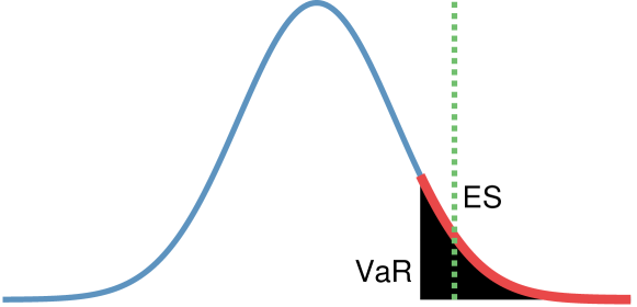
Figure 1: VaR and ES of a unit normal distribution at $\epsilon=0.1$

2.3 Stochastic Processes and Occupation Measures

Let $\{\mu_{t}\}\in\mathcal{M}_{+}(X)$ be a time-indexed sequence of probability distributions. Define $\mathcal{T}_{\tau}$ as a time-shifting (Feller) semigroup operator acting as $\mathcal{T}_{\tau}\mu_{t}=\mu_{t+\tau}$. The generator $\mathcal{L}_{\tau}$ of a stochastic processes associated with the distributions $\{\mu_{t}\}$ is a linear operator satisfying (for any test function $v(t,x)\in C([0,T]\times X)$ and in the domain of $\mathcal{L}$):

$$\mathcal{L}_{\tau}v=\lim_{\tau^{\prime}\rightarrow\tau}(\langle v(t+\tau^{\prime},x),\mu_{t+\tau^{\prime}}\rangle-\langle v(t,x),\mu_{t}\rangle)/\tau^{\prime}.$$ (7)

A discrete-time Markov stochastic process with parameter distribution $\xi(\lambda)\in\mathcal{M}_{+}(\Lambda)$ and time-step $\Delta t>0$ has a law and associated generator of

$$x[t+\Delta t] =f(t,x[t],\lambda[t]),\qquad\lambda[t]\sim\xi$$ (8)

$$\mathcal{L}_{\Delta t}v =\left(\int_{\Lambda}v(t+\Delta t,f(t,x,\lambda))d\xi(\lambda)-v(t,x)\right)/\Delta t.$$ (9)

The domain of $\mathcal{L}_{\Delta t}$ in (9) is $\mathcal{C}=C([0,T]\times X)$.

Itô SDEs are the unique class of continuous-time stochastic processes that are nonanticipative, have independent increments, and possess continuous sample paths [38]. Every Itô SDE has a definition in terms of a (possibly nonunique) drift function $f$, a diffusion function $g$, and an $n$-dimensional Wiener process $W$ as

$$dx=f(t,x)dt+g(t,x)d{W}.$$ (10)

This paper will involve stochastic trajectories evolving in a compact set $X$, starting within an initial set $X_{0}$ at time $0$. Letting $\tau_{X}$ be a stopping time (RV) associated with the first touch of the boundary $\partial X$, the strong SDE solution of (10) in times $t\in[0,T]$ starting at an initial point $x(0)\in X_{0}$ is

$$x(t)=x(0)+\int_{t=0}^{\tau_{X}\wedge T}f(t,x)dt+\int_{t=0}^{\tau_{X}\wedge T}g(t,x)d{W}.$$ (11)

Strong solutions of (11) (sequence of state-probability-distributions $\{\mu_{t}\}$ describing $x(t)$) are unique if there exists $C,D>0$ such that the following Lipschitz and Growth conditions hold for all $(t,x,x^{\prime})\in[0,T]\times X^{2}$ [38]:

$$D\lVert x-x^{\prime}\rVert_{2} \geq\lVert f(t,x)-f(t,x^{\prime})\rVert_{2}+\lVert g(t,x)-g(t,x^{\prime})\rVert_{2}$$

$$C(1+\lVert x\rVert_{2}) \geq\lVert f(t,x)\rVert_{2}+\lVert g(t,x)\rVert_{2}.$$ (12)

These Lipschitz and Growth conditions will be satisfied if $X$ is compact and $(f,g)$ are locally Lipschitz. The generator associated to (10) with domain $C^{1,2}([0,T]\times X)$ is

$$\mathcal{L}v(t,x)=\partial_{t}v+f(t,x)\cdot\nabla_{x}v+\frac{1}{2}g(t,x)^{T}\left(\nabla^{2}_{xx}v\right)g(t,x).$$ (13)

In the rest of this paper, we denote the domain of the generator $\mathcal{L}$ by $\mathcal{C}$, and will refer to stochastic processes by their generators ($x(t)$ or $\{\mu_{t}\}$ satisfy the stochastic process of $\mathcal{L}$ in time $T\wedge\tau_{X}$).

Let $\mu_{0}\in\mathcal{M}_{+}(X_{0})$ be an initial distribution, $t^{\prime}\in[0,T]$ be a terminal time, and $\tau=t^{\prime}\wedge\tau_{X}$ be an associated stopping time. The occupation measure $\mu\in\mathcal{M}_{+}([0,T]\times X)$ and stopping measure $\mu_{\tau}\in\mathcal{M}_{+}([0,T]\times X)$ of the stochastic processes $\mathcal{L}$ w.r.t. $\mu_{0}$ is $\forall A\subseteq[0,T],B\subseteq X$:

$$\mu(A\times B) =\int_{X_{0}}\int_{t=0}^{\tau}I_{A\times B}\left(t,x(t\mid x_{0})\right)dt\,d\mu_{0}(x_{0})$$ (14a)

$$\mu_{\tau}(A\times B) =\int_{X_{0}}I_{A\times B}\left(\tau,x(\tau\mid x_{0})\right)\,d\mu_{0}(x_{0}).$$ (14b)

The measures $(\mu_{0},\mu,\mu_{\tau})$ together obey a martingale relation [39]:

$$\langle v,\mu_{\tau}\rangle =\langle v(0,x),\mu_{0}(x)\rangle+\langle\mathcal{L}v,\mu\rangle \forall v\in\mathcal{C},$$ (15)

which can be equivalently expressed in shorthand form as

$$\mu_{\tau} =\delta_{0}\otimes\mu_{0}+\mathcal{L}^{\dagger}\mu.$$ (16)

The martingale relation in (16) is known as Dynkin’s formula [40] when $\mathcal{L}$ is the generator for SDE SDE. A relaxed occupation measure is a tuple $(\mu_{0},\mu,\mu_{\tau})$ satisfying (16) with $\langle 1,\mu_{0}\rangle=1$.

An optimal stopping problem to maximize the expectation of the reward $p(x)$ along trajectories of $\mathcal{L}$ is $P^{*}=\sup_{t^{\prime}\in[0,T]}\langle p(x),\mu_{t^{\prime}}(x)\rangle$. This stopping problem may be upper-bounded by an infinite-dimensional LP in measures

$$p^{*}= \ \sup\quad\langle p,\mu_{\tau}\rangle$$ (17a)

$$\mu_{\tau}=\delta_{0}\otimes\mu_{0}+\mathcal{L}^{\dagger}\mu$$ (17b)

$$\langle 1,\mu_{0}\rangle=1$$ (17c)

$$\mu,\mu_{\tau}\in\mathcal{M}_{+}([0,T]\times X).$$

The upper-bound is tight $(p^{*}=P^{*})$ when $p$ is continuous, $[0,T]\times X$ is compact, and closure conditions hold on the generator $\mathcal{L}$ [20] (to be reviewed in Section (3.1)). SDE trajectories under Lipschitz and Growth (12) conditions will satisfy these requirements.

3 Chance-Peak Problem Statement

This section presents the problem statement for the chance-peak problem, and will formulate the tail-bound and ES upper-bounding programs to peak-VaR estimation.

3.1 Assumptions

We will require the following assumptions:

• The spaces $[0,T]$ and $X$ are compact.

• Trajectories stop upon their first contact with $\partial X$.

• The state function $p$ is continuous on $X$.

• The initial measure $\mu_{0}$ satisfies $\langle 1,\mu_{0}\rangle=1$ and $\textrm{supp}(\mu_{0})\subseteq X$.

• The set $\mathcal{C}=\textrm{dom}(\mathcal{L})\subset\textrm{Hom}(C([0,T]\times X),C([0,T]\times X))$ contains $1\in\mathcal{C}$ with $\mathcal{L}1=0$.

• The set $\mathcal{C}$ can separate points and is closed under multiplication.

• There exists a countable basis $\{v_{k}\}\in\mathcal{C}$ such that every $(v,Av)$ with $v\in\mathcal{C}$ is contained in the (bounded pointwise closure of the) linear span of $\{(v_{k},\mathcal{L}v_{k})\}$.

Assumptions A5-A7 originate from the requirements of Condition 1 of [20]. Discrete-time Markov processes, SDEs, and Lévy processes in compact domains (A1, A2) will satisfy conditions A5-A7 [20]. Assumption A5 and (7) together imply that $\mathcal{L}t=1$.

3.2 VaR Problem

Problem 3.1.

The chance-peak problem that maximizes the $\epsilon$-VaR of $p$ is

$$P^{*}= \sup_{t^{*}\in[0,T]}\ \mathrm{VaR}_{\epsilon}(p{(x(t^{*}))})$$ (18a)

$$\text{$x(t)$ follows $\mathcal{L}$ from $t=0$ until }\ \tau_{X}\wedge t^{*}$$ (18b)

$$x(0)\sim\mu_{0}.$$ (18c)

4 Tail-Bound Program

This section solves the chance-peak problem 3.1 using tail-bounds by developing an infinite-dimensional SOCP in measures.

4.1 Tail-Bound Problem

We define $r$ as the constant factor multiplying against $\sigma$ in the Cantelli or VP expression of (2) as in

$${r_{C}} =\sqrt{(1/\epsilon)-1} {r_{VP}} =\sqrt{4/(9\epsilon)-1},$$ (19)

ensuring that the VP bound is used if and only if its $\epsilon\leq 1/6$ and unimodality conditions are satisfied. We also use the notation $\langle p^{2},\mu_{t^{*}}\rangle$ to denote the expectation $\mathbb{E}[p(x(t^{*}))^{2}]$.

Problem 4.1.

The tail-bound program upper-bounding (18) with constant $r$ is

$$P^{*}_{r}= \sup_{t^{*}\in[0,T]}r\sqrt{\langle p^{2},\mu_{t^{*}}\rangle-\langle p,\mu_{t^{*}}\rangle^{2}}+\langle p,\mu_{t^{*}}\rangle$$ (20a)

$$\text{$x(t)$ follows $\mathcal{L}$ from $t=0$ until }\ \tau_{X}\wedge t^{*}$$ (20b)

$$x(0)\sim\mu_{0}.$$ (20c)

4.2 Nonlinear Measure Program

Problem (20) can be converted into an infinite-dimensional nonlinear program in variables $(\mu_{\tau},\mu)$, given the initial distribution $\mu_{0}$ and the generator $\mathcal{L}$:

$$p^{*}_{r}= \sup r\sqrt{\langle p^{2},\mu_{\tau}\rangle-\langle p,\mu_{\tau}\rangle^{2}}+\langle p,\mu_{\tau}\rangle$$ (21a)

$$\mu_{\tau}=\delta_{0}\otimes\mu_{0}+\mathcal{L}^{\dagger}\mu$$ (21b)

$$\mu_{\tau},\ \mu\in\mathcal{M}_{+}([0,T]\times X).$$

Theorem 4.2.

Programs (21) and (20) are related by $p^{*}_{r}\geq P^{*}_{r}$ under assumptions A1, A2, A4.

Proof.

Let $t^{*}\in[0,T]$ be a terminal time with stopping time of $\tau^{*}=t^{*}\wedge\tau_{X}$. We can construct measures $(\mu,\mu_{\tau})$ to satisfy (21b) from the data in $(t^{*},\mathcal{L},\mu_{0})$. Specifically, let $\mu$ be the occupation measure of the stochastic process $\mathcal{L}$ starting from $\mu_{0}$ until time $\tau^{*}$, and let $\mu_{\tau}$ be the time-$\tau^{*}$ state distribution. The allowed stopping times $t^{*}\in[0,T]$ for (20) maps in a one-to-one manner on the feasible set of constraints (21), affirming that $p^{*}_{r}\geq P^{*}_{r}$. ∎

Remark 4.

A worst-case tail-bound $p^{*}_{r}$ for (21) can be found from an initial set $X_{0}\subseteq X$ by letting the initial condition $\mu_{0}$ be an optimization variable with the constraints $\mu_{0}\in\mathcal{M}_{+}(X_{0})$ and $\langle 1,\mu_{0}\rangle=1$.

Lemma 4.3.

Under assumptions (A1, A2, A4-7), to every $(\mu_{\tau},\mu)$ obeying (24b) there exists a stochastic process trajectory (20b) starting at $\mu_{0}$ and terminating at $\mu_{\tau}$ with an occupation measure of $\mu$.

Proof.

This lemma holds by Theorem 3.3 of [20] (under A1, A2, A5-7; noting that $[0,T]\times X$ is a complete metric space). ∎

Corollary 1.

The combination of Theorem 4.2 and Lemma 4.3 implies that $p^{*}_{r}=P^{*}_{r}$ under assumptions A1-A7.

4.3 Measure Second-Order Cone Program

This subsection will demonstrate how the nonlinear program in measures (21) may be equivalently expressed as an infinite-dimensional convex measure SOCP. We will use an SOC representation of the square-root to accomplish this conversion through the following lemma:

Lemma 4.4.

Define the objective (21a) as $J_{r}(a,b)=r\sqrt{b-a^{2}}+a$ under the substitutions $a=\langle p,\mu_{\tau}\rangle$ and $b=\langle p^{2},\mu_{\tau}\rangle$. Given any convex set ${K}\in\mathbb{R}\times\mathbb{R}_{+}$ with $(a,b)\in{K}$, the subsequent programs will possess the same optimal value:

$$\sup_{(a,b)\in{K}}a+r\sqrt{b-a^{2}}$$ (22)

$$\sup_{(a,b)\in{K},\ {c}\in\mathbb{R}}a+r{\,c}:\ ([1-b,2{c},2a],1+b)\in{\mathbb{L}}^{3}.$$ (23)

Proof.

We introduce a new variable $c$ as in $c\leq\sqrt{b-a^{2}}$, which implies that ${c}^{2}+a^{2}\leq b$. The SOC-equivalent form of $\sqrt{b-a^{2}}$ follows from [41, 42],

$$([1-b,2{c},2a],1+b)\in{\mathbb{L}}^{3}$$

$$\Longleftrightarrow\; (1-b)^{2}+4({c}^{2}+a^{2})\leq(1+b)^{2}$$

$$\Longleftrightarrow\; (1+b^{2})-2b+4({c}^{2}+a^{2})\leq(1+b^{2})+2b$$

$$\Longleftrightarrow\; 4({c}^{2}+a^{2})\leq 4b.$$

∎

Theorem 4.5.

The nonlinear program (21) has the same set of feasible solutions and optimal value as the following SOCP (given $(\mu_{0},\mathcal{L},r)$):

$$p^{*}_{r}= \sup\quad r{c}+\langle p,\mu_{\tau}\rangle$$ (24a)

$$\mu_{\tau}=\delta_{0}\otimes\mu_{0}+\mathcal{L}^{\dagger}\mu$$ (24b)

$${y}=[1-\langle p^{2},\mu_{\tau}\rangle,\ 2{c},\ 2\langle p,\mu_{\tau}\rangle]$$ (24c)

$$({y},1+\langle p^{2},\mu_{\tau}\rangle)\in{\mathbb{L}}^{3}$$ (24d)

$$\mu,\ \mu_{\tau}\in\mathcal{M}_{+}([0,T]\times X),u\in\mathbb{R},c\in\mathbb{R}^{3}.$$

Proof.

This equivalence follows from Lemma 4.4 by replacing the square-root in the objective (21a). The new optimization variables are $(\mu_{\tau},\mu,u,c)$. ∎

Corollary 2.

The SOCP in (24) is convex.

Proof.

Constraints (24b)-(24d) are convex (SOC for (24d) and affine for (24b)). The objective (24a) is linear in $({c},\mu_{\tau})$. ∎

4.4 Dual Second-Order Cone Program

The Lagrangian dual of (24) is a program with infinite-dimensional linear constraints and a finite-dimensional SOC constraint. This dual involves a function $v(t,x)\in\mathcal{C}([0,T]\times X)$ and a constant $u\in\mathbb{R}^{3}$ as variables.

We will use the following expression of (24) with an explicitly written SOC variable $z$ linked with linear constraints to the measures $(\mu_{0},\mu_{\tau},\mu)$.

Lemma 4.6.

The following program has the same optimal value as (24):

$$p^{*}_{r}= \sup\quad(r/2)z_{2}+\langle p,\mu_{\tau}\rangle$$ (25a)

$$z_{1}+\langle p^{2},\mu_{\tau}\rangle=1$$ (25b)

$$z_{3}-2\langle p,\mu_{\tau}\rangle=0$$ (25c)

$$z_{1}+z_{4}=2$$ (25d)

$$\mu_{\tau}-\mathcal{L}^{\dagger}\mu=\delta_{0}\otimes\mu_{0}$$ (25e)

$$z=([z_{1},z_{2},z_{3}],z_{4})\in\mathbb{L}^{3}$$

$$\mu,\ \mu_{\tau}\in\mathcal{M}_{+}([0,T]\times X).$$

Proof.

This formulation is obtained from (24) through the change of variable $z=(y,1+\langle p^{2},\mu_{\tau}\rangle)$ and the replacement of $c$ with $z_{2}/2$ using the second coordinate of constraint (24c). Equation (25d) is derived by adding the first coordinate of (24c) and the last coordinate of (24d).

∎

Theorem 4.7.

The dual program of (24) with weak duality $d^{*}_{r}\geq p^{*}_{r}$ under Assumptions A1-A3 is

$$d^{*}_{r}= \inf\quad u_{1}+2u_{3}+\int_{X_{0}}v(0,x_{0})d\mu_{0}(x_{0})$$ (26a)

$$\forall(t,x)\in[0,T]\times X:$$

$$\qquad\mathcal{L}v(t,x)\leq 0$$ (26b)

$$\forall(t,x)\in[0,T]\times X:$$

$$\qquad v(t,x)+u_{1}\,p^{2}(x)-2\,u_{2}\,p(x)\geq p(x)$$ (26c)

$$([u_{1}+u_{3},-(r/2),u_{2}],u_{3})\in{\mathbb{L}}^{3}$$ (26d)

$$u\in\mathbb{R}^{3},\ v\in\mathcal{C}([0,T]\times X).$$

Strong duality with $d^{*}_{r}=p^{*}_{r}$ holds under Assumptions A1-A4.

Proof.

Dual formulation: this formulation is obtained by applying the standard Lagrangian duality method to (25). $v$ is the Lagrange multiplier corresponding to constraint (25e), and $u$ is the Lagrange multiplier corresponding to constraints (25b)-(25d). Conversely, $\mu$ is the Lagrange multiplier corresponding to constraint (26b), $\mu_{\tau}$ is the Lagrange multiplier corresponding to constraint (26c), and $z$ is the Lagrange multiplier corresponding to (26d). The cost in (26a) corresponds to the right-hand sides of constraints (25b)-(25e), while the right-hand side of (26c) and the second coordinate $-(r/2)$ in (26d) correspond to the cost in (25a).

Strong duality: see Appendix B. ∎

This strong duality property is an important feature of the infinite-dimensional problem at hand: it means that one may equivalently solve moment relaxations of (25) and SOS tightenings of (26).

5 ES Program

This section poses LP LP in measures to solve the ES upper-bound to Problem 3.1.

5.1 ES Problem

The ES chance-peak problem replaces the VaR objective in (18a) with ES.

Problem 5.1.

The ES program that upper-bounds the chance-peak problem in (18) is

$$P^{*}_{c}= \sup_{t^{*}\in[0,T]}\mathrm{ES}_{\epsilon}(p(x(t^{*})))$$ (27a)

$$\text{$x(t)$ follows $\mathcal{L}$ from $t=0$ until }\ \tau_{X}\wedge t^{*}$$ (27b)

$$x(0)\sim\mu_{0}.$$ (27c)

5.2 ES reformulation

We begin by using the following lemma to reformulate the absolute-continuity-based ES definition in (5) into an equivalent domination-based LP in measures.

Lemma 5.2.

Let ${\mu},\nu\in\mathcal{M}_{+}(\mathbb{R})$ be measures such that $\nu\ll\mu$, and $\frac{d\nu}{d\mu}\leq 1$. Then there exists a slack measure ${\hat{\nu}}\in\mathcal{M}_{+}(\mathbb{R})$ such that ${\nu+\hat{\nu}=\mu}$.

Proof.

The measure ${\hat{\nu}}$ may be chosen with $\frac{d\hat{\nu}}{d\mu}=1-\frac{d\nu}{d\mu}$. This implies that ${\frac{d\nu}{d\mu}+\frac{d\hat{\nu}}{d\mu}}=1$, resulting in $\nu+\hat{\nu}=\mu$. ∎

Theorem 5.3.

The ES is the solution to the following LP in measures:

$$\mathrm{ES}_{\epsilon}(V)= \sup_{\nu,\hat{\nu}\in\mathcal{M}_{+}(\mathbb{R})}\langle\mathrm{id}_{\mathbb{R}},\nu\rangle$$ (28a)

$$\epsilon\nu+\hat{\nu}=\psi=V_{\#}\mathbb{P}$$ (28b)

$$\langle 1,\nu\rangle=1.$$ (28c)

Proof.

Equation (5c) may be divided through by $\epsilon$ to form $\epsilon{\frac{d\nu}{d\psi}=\frac{d(\nu\epsilon)}{d\psi}}\leq 1$. Given that $\epsilon>0$, the absolute continuity relation ${\nu\ll\psi}$ implies that $\epsilon{\nu\ll\psi}$. Lemma 5.2 is applied to the combination of $\epsilon{\nu\ll\psi}$ and ${\frac{d(\nu\epsilon)}{d\psi}}\leq 1$ to produce constraint (28b). This proves the conversion and equivalence of optima between (5) and (28).

∎

5.3 Measure Program

LP LP in measures will be created to upper-bound the ES program (27). The variables involved are the terminal measure $\mu_{\tau}$, the relaxed occupation measure $\mu$, the ES dominated measure ${\nu}$, and the ES slack measure ${\hat{\nu}}$.

$$p^{*}_{c}= \ \sup\quad\langle\mathrm{id}_{\mathbb{R}},\nu\rangle$$ (29a)

$$\mu_{\tau}=\delta_{0}\otimes\mu_{0}+\mathcal{L}^{\dagger}\mu$$ (29b)

$$\langle 1,\nu\rangle=1$$ (29c)

$$\epsilon\nu+\hat{\nu}=p_{\#}\mu_{\tau}$$ (29d)

$$\mu,\mu_{\tau}\in\mathcal{M}_{+}([0,T]\times X)$$

$$\nu,\hat{\nu}\in\mathcal{M}_{+}(\mathbb{R}).$$

Theorem 5.4.

Program (29) upper-bounds (27) with $p^{*}\geq P^{*}$ under assumptions A2-A4.

Proof.

We will prove this upper-bound by constructing a measure representation of an SDE trajectory in (27). Let $t^{*}\in[0,T]$ be a stopping time. Define $\mu_{\tau}=\mu_{t^{*}}$ as the state (probability) distribution of the process (27b) at time $t^{*}$ (accounting for the stopping time $\tau_{X}\wedge t^{*}$). Let $\mu$ be the occupation measure of this SDE connecting together the initial distribution $\mu_{0}$ and the terminal distribution $\mu_{t^{*}}$. The measures ${\nu,\hat{\nu}}$ are set in accordance with Theorem 5.3 under $\Omega=[0,T]\times X$, $\mathbb{P}=\mu_{t^{*}}$ and $V=p$ (hence ${\psi}=p_{\#}\mu_{t^{*}}$). The upper-bound holds because every process trajectory has a measure construction. ∎

Theorem 5.5.

There is no relaxation gap between (29) and (27) $(p^{*}_{c}=P^{*}_{c})$ under assumptions A1-A7.

Proof.

Every $(\mu_{\tau},\mu)$ is supported on an stochastic process trajectory by Lemma 4.3. The objective in (29a) will equal the ES by Theorem 5.3 given that $p_{\#}\mu_{\tau}$ is a probability distribution. ∎

Remark 5.

To the best of our knowledge, there does not appear to be a consistent comparison between the VP bound and the ES of a unimodal distribution.

5.4 Function Program

The functional LP dual to (29) will have variables $u\in\mathbb{R}$, $v\in\mathcal{C}([0,T]\times X)$ and ${w}\in C(\mathbb{R})$ (dual to (29b)-(29d)).

Theorem 5.6.

The strong-dual program of (29) with duality $d^{*}_{c}{=}p^{*}_{c}$ under A1-A4 is

$$d^{*}_{c}= \inf\quad{u+\langle v(0,\bullet),\mu_{0}\rangle}$$ (30a)

$$\mathcal{L}v\leq 0$$ (30b)

$$v\geq{w\,\circ\,}p$$ (30c)

$${u\ +\ }\epsilon\,{w}\geq\mathrm{id}_{\mathbb{R}}$$ (30d)

$${w}\geq 0$$ (30e)

$${u\in\mathbb{R}},v\in\mathcal{C}{,w\in C(\mathbb{R})}.$$ (30f)

Proof.

See Appendix C. ∎

6 Finite Moment Program

This section will apply the moment-SOS hierarchy of SDPs to develop upper-bounds of (24) and (29).

6.1 Review of Moment-SOS Hierarchy

Refer to [21] for a more complete introduction to concepts reviewed in this subsection. Letting $\mathbf{m}=\{\mathbf{m}_{\alpha}\}_{\alpha\in\mathbb{N}^{n}}\in\mathbb{R}^{\mathbb{N}^{n}}$ be a multi-indexed vector, we can define a Riesz linear functional $L_{\mathbf{m}}:\ \mathbb{R}[x]\rightarrow\mathbb{R}$ as

$$\begin{array}[]{ccc}p(x)=\sum\limits_{\alpha\in\mathbb{N}^{n}}p_{\alpha}x^{\alpha}&\longmapsto&\textstyle L_{\mathbf{m}}p=\sum\limits_{\alpha\in\mathbb{N}^{n}}p_{\alpha}\mathbf{m}_{\alpha}.\end{array}$$ (31a)

For any measure $\mu\in\mathcal{M}_{+}(X)$ and multi-index $\alpha\in\mathbb{N}^{n}$, the $\alpha$-moment of $\mu$ is $\mathbf{m}_{\alpha}=\langle x^{\alpha},\mu\rangle$. The infinite-dimensional moment sequence $\mathbf{m}=\{\mathbf{m}_{\alpha}\}_{\alpha\in\mathbb{N}^{n}}$ is related to the linear functional $L_{\mathbf{m}}$ by

$$\forall p\in\mathbb{R}[x],\quad L_{\mathbf{m}}p=\langle p,\mu\rangle.$$ (31b)

Given a moment sequence $\mathbf{m}\in\mathbb{R}^{\mathbb{N}^{n}}$ and a polynomial $h\in\mathbb{R}[x]$, a localizing bilinear functional can be defined by $L_{h\mathbf{m}}:\mathbb{R}[x]\times\mathbb{R}[x]\longrightarrow\mathbb{R}$ by

$$L_{h\mathbf{m}}=(p,q)\longmapsto L_{\mathbf{m}}(hpq).$$ (32)

The cone of polynomials $\mathbb{R}[x]$ can be treated as a vector space with a linear basis $(e_{i})_{i\in\mathbb{N}}$ (e.g. $e_{i}(x)=x^{\alpha_{i}}$ with $\{\alpha_{i}\}_{i\in\mathbb{N}}=\mathbb{N}^{n}$ and a monomial ordering $|\alpha_{i}|<|\alpha_{j}|\Rightarrow i<j$). The bilinear functional $L_{h\mathbf{m}}$ has a representation as a quadratic form operating on an infinite-size localizing matrix $\mathbb{M}[h\mathbf{m}]$ with $\mathbb{M}[h\mathbf{m}]=(L_{\mathbf{m}}(h\,e_{i}\,e_{j}))_{i,j\in\mathbb{N}}$. The expression for $\mathbb{M}[h\mathbf{m}]$ when $\{e_{j}\}$ is the set of ordered monomials leads to

$$\mathbb{M}[h\mathbf{m}]_{i,j}=L_{\mathbf{m}}(hx^{\alpha_{i}}x^{\alpha_{j}})=\sum_{\beta\in\mathbb{N}^{n}}h_{\beta}\mathbf{m}_{\alpha_{i}+\alpha_{j}+\beta}.$$ (33)

BSA Basic Semialgebraic (BSA) set $\mathbb{K}=\{x\mid h_{k}(x)\geq 0:\ k=1..N_{c}\}$ is a set defined by a finite number of bounded-degree polynomial inequality constraints $h_{k}(x)\geq 0$. We refer to any set $\mathbb{K}$ that has $h_{1}(x)=1$ and $h_{N_{c}}=R-\lVert x\rVert_{2}^{2}$ with $R>0$ as satisfying ‘ball constraints,’ and note that such an $R>0$ can be chosen for any compact set. For any set obeying ball constraints, then there exists a representing measure $\mu$ for the sequence of numbers (pseudomoments) $\mathbf{m}$ if each localizing matrix is Positive Semidefinite (PSD):

$$\forall\mathbb{N},k=1..N_{c},\quad\mathbb{M}[h_{k}\mathbf{m}]\succeq 0.$$ (34)

For a finite $d\in\mathbb{N}$, a sufficient condition for (34) to hold is that the upper-left corner of $\mathbb{M}[h_{k}\mathbf{m}]$ containing moments up to degree $2d$ (expressed as $\mathbb{M}_{d}[h_{k}\mathbf{m}]$) is PSD. The truncated matrix $\mathbb{M}_{d}[h_{k}\mathbf{m}]$ represents the bilinear operator $L_{h\mathbf{m}}$ in the finite-dimensional vector space $\mathbb{R}[x]_{\leq d}$, and has size $\binom{n+d}{d}$ when $\{e_{i}\}$ is a monomial basis.

We will define the degree-$d$ block-diagonal matrix composed of localizing matrices for constraints of $\mathbb{K}$ as

$$\mathbb{M}_{d}[\mathbb{K}\mathbf{m}]=\mathrm{diag}(\mathbb{M}_{d-\lceil d_{k}/2\rceil}[h_{k}\mathbf{m}])_{k=1..N_{c}}.$$ (35)

The moment-SOS hierarchy is the process of raising the degree $d$ to $\infty$ while imposing that the matrix in (35) is PSD.

6.2 Chance-Peak Moment Setup

We require polynomial-structuring assumptions in order to approximate (24) and (29) using the moment-SOS hierarchy:

• The sets $X_{0}$ and $X$ are both BSA with ball constraints.

• The generator $\mathcal{L}$ satisfies $\forall v\in\mathbb{R}[t,x],\ \mathcal{L}v\in\mathbb{R}[t,x]$.

• The objective function $p(x)$ is also polynomial.

Let $(\mathbf{m},\mathbf{m}^{\tau})$ be pseudomoments for the optimization variables $(\mu,\mu_{\tau})$. For each $\alpha\in\mathbb{N}^{n}$ and $\beta\in\mathbb{N}$ producing the monomial $x^{\alpha}t^{\beta}$, we define the operator $\mathcal{D}_{\alpha\beta}$ as the moment expression for the generator $\mathcal{L}$ with

$$\mathcal{D}_{\alpha\beta}(\mathbf{m},\mathbf{m}^{\tau})=\mathbf{m}^{\tau}_{\alpha\beta}-L_{\mathbf{m}}(\mathcal{L}(x^{\alpha}t^{\beta})).$$ (36)

We further define a dynamics degree $D$ as a function of the degree $d$ such that

$$\deg x^{\alpha}t^{\beta}\leq 2d\implies\deg\mathcal{L}x^{\alpha}t^{\beta}\leq 2D.$$ (37)

6.3 Tail-Bound Moment Program

Problem 6.1.

For any $d\in\mathbb{N}$ such that $2d\geq\deg p$, the order-$d$ Linear Matrix Inequality (LMI) in pseudomoments to upper-bound (24) given $\mu_{0}$ is

$$p^{*}_{r,d}= \max\quad r{c}+L_{\mathbf{m}^{\tau}}p$$ (38a)

$${c}\in\mathbb{R},\mathbf{m}\in\mathbb{R}^{{}^{\binom{2D+n+1}{n+1}}},\mathbf{m}^{\tau}\in\mathbb{R}^{{}^{\binom{2d+n+1}{n+1}}}$$

$$\mathcal{D}_{\alpha\beta}(\mathbf{m},\mathbf{m}^{\tau})=\delta_{\beta 0}\langle x^{\alpha},\mu_{0}\rangle$$

$$\qquad\forall(\alpha,\beta)\in\mathbb{N}^{n+1}\quad\text{s.t.}\quad|\alpha|+\beta\leq 2d$$ (38b)

$${y}=[1-L_{\mathbf{m}^{\tau}}(p^{2}),\ 2{c},\ 2L_{\mathbf{m}^{\tau}}p]$$ (38c)

$$({y},1+L_{\mathbf{m}^{\tau}}(p^{2}))\in{\mathbb{L}}^{3}$$ (38d)

$$\mathbb{M}_{d}[([0,T]\times X)\mathbf{m}^{\tau}]\succeq 0$$ (38e)

$$\mathbb{M}_{D}[([0,T]\times X)\mathbf{m}]\succeq 0,$$ (38f)

in which the Kronecker symbol $\delta_{\beta 0}$ is $1$ if $\beta=0$ and is $0$ otherwise. Constraint (38b) is a finite-dimensional truncation of the infinite-dimensional martingale relation (24b).

We now prove that all optimization variables of (24) are bounded in order to prove convergence of (38) as $d\rightarrow\infty$.

Lemma 6.2.

The variables $(\mu,\mu_{\tau},{c})$ in any feasible solution of (24) are bounded under A1-A7.

Proof.

A measure is bounded if all of its moments are bounded (finite). A sufficient condition for boundedness of measures to hold is if the measure is supported on a compact set and that it has finite mass. Compact support of $(\mu,\mu_{\tau})$ is ensured by A1. Substitution of $v(t,x)=1$ into (24b) leads to $\langle 1,\mu_{\tau}\rangle=\langle 1,\mu_{0}\rangle=1$ by A4-5. The moments $\langle p,\mu_{\tau}\rangle$ and $\langle p^{2},\mu_{\tau}\rangle$ are therefore finite under A1 and A3, which implies that $c$ is bounded as well. Applying $v(t,x)=t$ yields $\langle 1,\mu\rangle\leq\langle t,\mu_{\tau}\rangle\leq T$, which implies that $\langle 1,\mu\rangle$ is finite by A5. All variables are therefore bounded.

∎

Theorem 6.3.

Under assumptions A1-A10, (38) inherits the strong duality property of its infinite-dimensional counterpart (24), and its optima will converge to (24) i.e. $\lim_{d\rightarrow\infty}p^{*}_{r,d}=p^{*}_{r}$.

Proof.

Strong duality is proved almost identically in the finite dimensional setting as in the infinite dimensional setting of Theorem 4.7 by using the same arguments as in the proof of [43, Proposition 6].

Convergence is a direct consequence of [43, Corollary 8] (when extending to the case with finite-dimensional SOC variables) through Lemma 6.2. ∎

Remark 6.

The relation $p^{*}_{d}\geq p^{*}_{r}\geq P^{*}_{r}$ will still hold when $[0,T]\times X$ is noncompact (violating A1 and A5), but it may no longer occur that $\lim_{d\rightarrow\infty}p^{*}_{r,d}=p^{*}_{r}$ (the conditions Lemma 6.3 will no longer apply).

6.4 CVAR Moment Program

Let $(\mathbf{m},\mathbf{m}^{\tau},{\mathbf{n}},\hat{{\mathbf{n}}})$ be respective moment sequences of the measures $(\mu,\mu_{\tau},{\nu,\hat{\nu}})$. We define the operator $\mathcal{E}_{k}(\mathbf{m}^{\tau},{\mathbf{n}},\hat{{\mathbf{n}}})$ for ${k}\in\mathbb{N}$ as the moment counterpart of the operator in constraint (29d):

$$\mathcal{E}_{k}(\mathbf{m}^{\tau},{\mathbf{n}},\hat{{\mathbf{n}}})=L_{\mathbf{m}^{\tau}}(p(x)^{k})-\epsilon{\mathbf{n}}_{k}-\hat{{\mathbf{n}}}_{k}.$$ (39)

The associated ES degree ${\Delta}$ is

$${\Delta}=\lfloor d/\deg p\rfloor.$$ (40)

Problem 6.4.

For each degree $d\geq\deg p$, the order-$d$ moment LMI that upper-bounds the ES LP (29) given the distribution $\mu_{0}$ is

$$p^{*}_{c,d}= \max L_{{\mathbf{n}}}q$$ (41a)

$$\mathbf{m}\in\mathbb{R}^{{}^{\binom{2D+n+1}{n+1}}},\mathbf{m}^{\tau}\in\mathbb{R}^{{}^{\binom{2d+n+1}{n+1}}}$$

$${\mathbf{n}}\in\mathbb{R}^{2{\Delta}+1},\ \hat{{\mathbf{n}}}\in\mathbb{R}^{2{\Delta}+1}$$

$$\forall(\alpha,\beta)\in\mathbb{N}^{n+1}\quad\text{s.t.}\quad|\alpha|+\beta:\leq 2d$$

$$\qquad\mathcal{D}_{\alpha\beta}(\mathbf{m},\mathbf{m}^{\tau})=\delta_{\beta 0}\langle x^{\alpha},\mu_{0}\rangle\qquad$$ (41b)

$$\mathcal{E}_{k}(\mathbf{m}^{\tau},{\mathbf{n}},\hat{{\mathbf{n}}})=0\qquad\forall{k}\in 0..(2{\Delta})$$ (41c)

$${\mathbf{n}}_{0}=1$$ (41d)

$$\mathbb{M}_{d}[([0,T]\times X)\mathbf{m}^{\tau}]\succeq 0$$ (41e)

$$\mathbb{M}_{D}[([0,T]\times X)\mathbf{m}]\succeq 0$$ (41f)

$$\mathbb{M}_{\Delta}[{[\hat{p},\check{p}]\mathbf{n}}]\succeq 0$$ (41g)

$$\mathbb{M}_{\Delta}[{[\hat{p},\check{p}]\mathbf{n}}]\succeq 0.$$ (41h)

The symbol $\delta_{\beta 0}$ is the Kronecker Delta ($1$ if $\beta=0$ and $0$ otherwise). Constraints (41b) and (41c) are finite-dimensional truncations of constraints (29b) and (29d) respectively.

Remark 7.

The redundant support constraints in (41g),(41h) are added to ensure that the Archimedean condition is satisfied for each moment sequence support.

Theorem 6.5.

All measures $\mu,\mu_{\tau},{\nu,\hat{\nu}}$ are bounded under A1-A4.

Proof.

This boundedness will be proved by showing that the mass of each measure is bounded and their support sets are compact.

Compactness: The measures $\mu_{\tau},\mu$ have compact support under A1. The quantities ${\hat{p}}=\min_{x\in X}p(x)$ and ${\check{p}}=\max_{x\in X}p(x)$ are each finite and attained under A1 and A3. The measure $p_{\#}\mu_{\tau}$ has support inside the compact set $[{\hat{p}},{\check{p}}]$ given that $\textrm{supp}(\mu_{\tau})\subseteq[0,T]\times X$. Both ${\nu}$ and ${\hat{\nu}}$ are nonnegative measures with $\epsilon>0$, so (29d) ensures that $\textrm{supp}(\nu)\subseteq[{\hat{p}},{\check{p}}]$ and $\textrm{supp}(\hat{\nu})\subseteq[{\hat{p}},{\check{p}}]$.

Bounded Mass: The mass of ${\nu}$ is set to 1 by (29c). Passing a test function $v(t,x)=1$ through (29b) results in $\langle 1,\mu_{\tau}\rangle=\langle 1,\mu_{0}\rangle$, which equals 1 by A4. Substitution of $v(t,x)=t$ through the same constraint yields $0+\langle 1,\mu\rangle=\langle t,\mu_{\tau}\rangle\leq T$. Given that $\mu_{\tau}$ is a probability measure, it holds that $p_{\#}\mu_{\tau}$ is also a probability measure. Finally, we analyze the mass of $\hat{\nu}$ with (29d):

$$\langle 1,\hat{\nu}\rangle =\langle 1,p_{\#}\mu_{\tau}-\epsilon\nu\rangle$$

$$=\langle 1,p_{\#}\mu_{\tau}\rangle-\epsilon\langle 1,\nu\rangle$$

$$=1-\epsilon<\infty.$$

All nonnegative measures have compact support and bounded masses under A1-A4, proving the theorem. ∎

Theorem 6.6.

The Cantelli $(r=\sqrt{1-1/\epsilon})$ program from (24) with objective $p^{*}_{r}$ will upper-bound the ES program (29) by $p^{*}_{r}\geq p^{*}_{c}$.

Proof.

This holds by Equation (5) of [35]. For a general univariate random variable $V\sim\psi\in\mathcal{M}_{+}(\mathbb{R})$ with variance $\sigma=\sqrt{\mathbb{E}[V^{2}]-\mathbb{E}[V]^{2}}$, the Cantelli bound is related to ES by

$${\mathbb{E}[V]}+\sigma\sqrt{1/\epsilon-1}\geq{\mathrm{ES}_{\epsilon}(V)\geq\mathrm{VaR}_{\epsilon}(V)}.$$ (42)

The Cantelli bound obtains the worst-case ES among all possible distributions agreeing with the given first and second moments [4]. ∎

Theorem 6.7.

The upper bounds of (41) will satisfy $p^{*}_{d}\geq p^{*}_{d+1}\geq...\geq p^{*}$ and $\lim_{d\rightarrow\infty}p^{*}=P^{*}$ under assumptions A1-A10.

Proof.

Boundedness and convergence will occur through Corollary 8 of [43] (all sets are Archimedean, all data is polynomial, measure solutions are bounded by Theorem (6.5), and the true objective value is finite). ∎

6.5 Computational Complexity

In Problem (38), the computational complexity mostly depends on the number and size of the matrix blocks involved in LMI constraints (38e,38f), which in turn depend on the number and degrees of polynomial inequalities describing $X$ (the higher $d_{k}=\deg(h_{k})$, the smaller $\mathbb{M}_{d-\lceil d_{k}/2\rceil}[h\mathbf{m}]$). At order-$d$, the maximum size of localizing matrices is $\binom{n+1+D}{D}$. This same analysis occurs for Problem (41) with respect to the LMI constraints (41e)-(41h).

Problems (38) and (41) must be converted to SDP-standard form by introducing equality constraints between the entries of the moment matrices in order to utilize symmetric-cone Interior Point Methods (e.g., Mosek [44]). The per-iteration complexity of SDP SDP involving a single moment matrix of size $\binom{n+d}{d}$ scales as $n^{6d}$ [26]. The scaling of SDP SDP with multiple moment and localizing matrices generally depends on the maximal size of any PSD matrix. In our case, this size is at most $\binom{n+1+d}{d}$ with a scaling impact of $(n+1)^{6d}$ or $d^{4(n+1)}$. The complexity of using this chance-peak routine increases in a jointly polynomial manner with $d$ and $n$.

7 Extensions

This section outlines extensions to the developed chance-peak framework. The formulas in this section will focus on the ES programs, but similar expressions may be derived for the tail-bound programs.

7.1 Switching

The ES-peak scheme may also be applied to switched stochastic systems. The methods outlined in this section are an extension of the ODE approach from [25], and are similar to duals of constraints found in [28]. Assume that there are $N_{s}\in\mathbb{N}$ subsystems indexed by $\ell=1..N_{s}$, each with an individual generator $\mathcal{L}_{\ell}$. As an example, a switched system with SDE subsystems $\ell=1..N_{s}$ could have individual dynamics

$$dx =f_{\ell}(t,x)dt+g_{\ell}(t,x)$$ (43)

and have associated generators $\mathcal{L}_{\ell}$ mapping $\forall v\in C^{1,2}([0,T]\times X)=\mathcal{C}([0,T]\times X),\forall\ell=1..N_{s}$:

$$\mathcal{L}_{\ell}v(t,x) =\partial_{t}v+f_{\ell}\cdot\nabla_{x}v+g_{\ell}^{T}(\nabla_{xx}^{2}v)g_{\ell}/2.$$ (44)

A switched trajectory is a distribution $x(t)$ and a switching function $S:[0,T]\rightarrow(1..N_{s})$ under the constraint that $x(t)$ satisfies (43) whenever $S(t)=\ell$ (the $\ell$-th subsystem is active). A specific trajectory of a switched process starting from an initial point $x_{0}\in X$ will be expressed as $x(t\mid x_{0},S)$. No dwell time constraints are imposed on the switching sequence $S$; instead, switching can occur arbitrarily quickly in time.

Let $\mu\in\mathcal{M}_{+}([0,T]\times X)$ be the total occupation measure of the switched process trajectory $x(t\mid x_{0},S)$. The total occupation measure may be split into disjoint subsystem occupation measures $\forall\ell:\ \mu_{\ell}\in\mathcal{M}_{+}([0,T]\times X)$ under the relation $\sum_{\ell=1}^{N_{s}}\mu_{\ell}=\mu$. The mass of a subsytem’s occupation measure $\langle 1,\mu_{\ell}\rangle$ is the total amount of time that the trajectory $x(t\mid x_{0},S)$ spends in subsystem $S(t)=\ell$.

The martingale equation (generalization of Dynkin’s (16)) for switching-type uncertainty is

$$\mu_{\tau}=\delta_{0}\otimes\mu_{0}+\textstyle\sum_{\ell=1}^{N_{s}}\mathcal{L}_{\ell}^{\dagger}\mu_{\ell}.$$ (45)

The ES-peak problem in (29) modified for switching uncertainty is

$$p^{*}= \ \sup\quad\langle\mathrm{id}_{\mathbb{R}},\nu\rangle$$ (46a)

$$\mu_{\tau}=\delta_{0}\otimes\mu_{0}+\textstyle\sum_{\ell=1}^{L}\mathcal{L}_{\ell}^{\dagger}\mu_{\ell}$$ (46b)

$$\langle 1,\nu\rangle=1$$ (46c)

$$\epsilon\nu+\hat{\nu}=p_{\#}\mu_{\tau}$$ (46d)

$$\forall\ell\in 1..L:\mu_{\ell}\in\mathcal{M}_{+}([0,T]\times X)$$ (46e)

$$\mu_{\tau}\in\mathcal{M}_{+}([0,T]\times X)$$ (46f)

$$\nu,\hat{\nu}\in\mathcal{M}_{+}(\mathbb{R}).$$ (46g)

7.2 Distance Estimation

The ES-peak methodology developed in this paper can be applied towards bounding (probabilistically) the distance of closest approach to an unsafe set. Let $X_{u}\subset X$ be an unsafe set, and let ${(x,x^{\prime})\mapsto\,}c(x,{x^{\prime}})$ be a metric in $X$. The point-set distance function with respect to $X_{u}$ is $c(x;X_{u})=\inf_{{x^{\prime}}\in X_{u}}c(x,{x^{\prime}})$.

The $\epsilon$-ES distance program may be expressed as (29) with an infimal (rather than supremal) objective $p(x)=c(x;X_{u})$. Because the objective $c({\bullet};X_{u})$ is not generally polynomial (even when $c$ is polynomial), the LMI (38) cannot directly be posed in terms of $c({\bullet};X_{u})$. One method to maintain a polynomial structure is to add time-constant states $dx_{u}=\mathbf{0}dt+\mathbf{0}dw$ to dynamics (10) in $x$ and form the state support set $(x,{x_{u}})\in X\times X_{u}$. When $X_{u}$ is full-dimensional inside $X\subset\mathbb{R}^{n}$, the occupation measure $\mu\in\mathcal{M}_{+}([0,T]\times X\times{X_{u}})$ will have a moment matrix of size $\binom{1+2n+d}{d}$ at each fixed degree $d$.

This size can be reduced using the method in [45], in which the peak measure $\hat{\mu}_{\tau}\in\mathcal{M}_{+}([0,T]\times X\times{X_{u}})$ is decomposed into a joint measure $\eta\in\mathcal{M}_{+}(X\times{X_{u}})$ and a peak measure $\mu_{\tau}\in\mathcal{M}_{+}([0,T]\times X)$ that have equal $x$ marginals. The resultant ES-distance LP is

$$c^{*}= \ \inf\quad\langle\mathrm{id}_{\mathbb{R}},\nu\rangle$$ (47a)

$$\mu_{\tau}=\delta_{0}\otimes\mu_{0}+\mathcal{L}^{\dagger}\mu$$ (47b)

$$\forall\phi\in C(X):$$ (47c)

$$\quad\int_{[0,T]\times X}\phi(x)\;d\mu_{\tau}(t,x)=\int_{X\times Y}\phi(x)\;d\eta(x,y)$$

$$\langle 1,\nu\rangle=1$$ (47d)

$$\epsilon\nu+\hat{\nu}=c_{\#}\mu_{\tau}$$ (47e)

$$\mu,\mu_{\tau}\in\mathcal{M}_{+}([0,T]\times X)$$

$$\nu,\hat{\nu}\in\mathcal{M}_{+}(\mathbb{R})$$

$$\eta\in\mathcal{M}_{+}(X\times X_{u}).$$

Constraint (47c) enforces equality in the $x$-marginals between $\mu_{\tau}$ and $\eta$. Constraint (47e) is a distance analogue of the pushforward ES constraint in (29d). The Moment matrices of $\eta$ and $\mu$ respectively in the LMI program derived from (47) have sizes $\binom{2n+d}{d}$, $\binom{n+1+\tilde{d}}{\tilde{d}}$, and $({\Delta}+1)$. Unfortunately, the exponentiation operation $\langle c^{k},\eta\rangle$ causes mixed multiplications in variables even when $c$ is additively separable as $c(x,y)=\sum_{i=1}^{n}c_{i}(x_{i},y_{i})$ (Section V of [46]), thus forbidding the application of correlative sparsity [47] to reduce the complexity of LMIs from (47).

8 Numerical Examples

All experiments were written in MATLAB (2022a) and require Mosek [44] and YALMIP [48] dependencies. Monte Carlo (MC) sampling is conducted with 50,000 sample paths (with SDE parameters of antithetic sampling and a spacing of $\Delta t=10^{-3}$) to approximate VaR and ES estimates. All experiments are accompanied by tables of chance-peak bounds and solver times. Files to generate examples are available at https://github.com/Jarmill/chance_peak (tail-bound Cantelli/VP) and https://github.com/Jarmill/cvar_peak (ES).

8.1 Two States

The first experiment is a cubic polynomial SDE from Example 1 of [27]:

$$dx=\begin{bmatrix}x_{2}\\ -x_{1}-x_{2}-\frac{1}{2}x^{3}_{1}\end{bmatrix}dt+\begin{bmatrix}0\\ 0.1\end{bmatrix}dW.$$ (48)

Chance-peak maximization of $p(x)=-x_{2}$ will occur starting at the point (Dirac-delta initial measure $\mu_{0}$) $X_{0}=[1,1]$ in a state set of $X=[-1,2]\times[-1,1.5]$ and time horizon of $T=5$. Figure 2 displays trajectories of (48) in cyan, starting from the black-circle point $X_{0}$. Four of these trajectory sample paths are marked in non-cyan colors.

The ‘mean’ row of Tables 1 and 3 display upper-bounds on the mean as solved by SDP truncations of (17). The bounds at $\epsilon=\{0.15,0.1,0.05\}$ for Table 1 are acquired by using the VP expression in (2b) and solving the SDPs obtained from (38). Table 3 displays bounds from SDPs derived from the ES LMI (41). The dash-dot red, dotted black, and solid red lines in Figure 2 are the mean, $\epsilon=0.15$ ES, and $\epsilon=0.15$ VP bounds respectively at order 6. All subsequent plots will retain this coloring and styling scheme for the mean, ES, and VP bounds. The top-right entry of Table 3 (and all similar tables) are omitted to reduce confusion between the $\epsilon=0.5$ VAR bound (which equals the mean) and the $\epsilon=0.5$ ES bound (which can exceed the mean).

Table 1: VP Chance-Peak estimation of the Stochastic Flow System (48) to maximize $p(x)=-x_{2}$

order	2	3	4	5	6	VaR MC
$\epsilon=0.5$	0.8818	0.8773	0.8747	0.8745	0.8744	0.8559
$\epsilon=0.15$	1.6660	1.6113	1.5842	1.5771	1.5740	0.9142
$\epsilon=0.1$	2.0757	1.9909	1.9549	1.9461	1.9427	0.9279
$\epsilon=0.05$	2.9960	2.8441	2.7904	2.7772	2.7715	0.9484

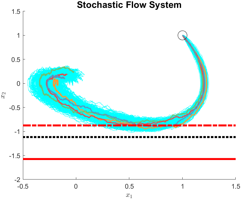
Figure 2: Trajectories of (48) with mean (dash-dot red), ES $\epsilon=0.15$ (dotted black), and VP $\epsilon=0.15$ (solid red) bounds

Table 2: Solver time (seconds) to compute Table 1

order	2	3	4	5	6
$\epsilon=0.5$	0.380	0.449	0.625	1.583	4.552
$\epsilon=0.15$	0.262	0.443	0.727	2.756	5.586
$\epsilon=0.1$	0.268	0.380	1.364	2.882	3.143
$\epsilon=0.05$	0.242	0.390	1.261	2.923	7.539

Table 3: ES Chance-Peak estimation of the Stochastic Flow System (48) to maximize $p(x)=-x_{2}$

order	2	3	4	5	6	ES MC
mean	0.8818	0.8773	0.8747	0.8745	0.8744
$\epsilon=0.15$	1.2500	1.2500	1.1655	1.1313	1.1170	0.9432
$\epsilon=0.1$	1.2500	1.2500	1.2116	1.1666	1.1466	0.9546
$\epsilon=0.05$	1.2500	1.2500	1.2500	1.2266	1.1959	0.9720

Table 4: Solver time (seconds) to compute Table 3

order	2	3	4	5	6
mean	0.619	0.504	0.558	2.862	1.652
$\epsilon=0.15$	0.363	0.402	0.399	1.341	2.016
$\epsilon=0.1$	0.357	0.442	0.417	1.054	2.093
$\epsilon=0.05$	0.414	0.393	0.399	0.579	2.534

8.2 Three States

A stochastic version of the Twist dynamics in [45] is:

$$dx=\begin{bmatrix}-2.5x_{1}+x_{2}-0.5x_{3}+2x_{1}^{3}+2x_{3}^{3}\\ -x_{1}+1.5x_{2}+0.5x_{3}-2x_{2}^{3}-2x_{3}^{3}\\ 1.5x_{1}+2.5x_{2}-2x_{3}-2x_{1}^{3}-2x_{2}^{3}\end{bmatrix}dt+\begin{bmatrix}0\\ 0\\ 0.1\end{bmatrix}dW.$$ (49)

This example applies the chance-peak setting towards maximization of $p(x)=x_{3}$, with an initial condition of $X_{0}=[0.5,0,0]$ and a state set $X=[-0.6,0.6]\times[-1,1]\times[-1,1.5]$ and $T=5$. VP and ES bounds from the (17) and (38) SDPs are written in Tables 5 and 7, similar in format to Tables 1 and 3. Trajectories and bounds are plotted in 3 beginning from the black-circle $X_{0}$. The three planes are order-6 bounds at $\epsilon=0.15$, in which the top solid red plane is the VP bound, the translucent black plane is the $\epsilon=0.15$ ES bound at order 6, and the translucent red plane is the mean bound on $x_{3}$.

Table 5: VP Chance-Peak estimation of the Stochastic Twist System (49) to maximize $p(x)=x_{3}$

order	2	3	4	5	6	VaR MC
$\epsilon=0.5$	0.9100	0.8312	0.8231	0.8211	0.8201	0.7206
$\epsilon=0.15$	1.6097	1.4333	1.3545	1.3318	1.3202	0.7685
$\epsilon=0.1$	1.9707	1.7453	1.6283	1.5877	1.5739	0.7801
$\epsilon=0.05$	2.7834	2.4426	2.2333	2.1622	2.1267	0.7970

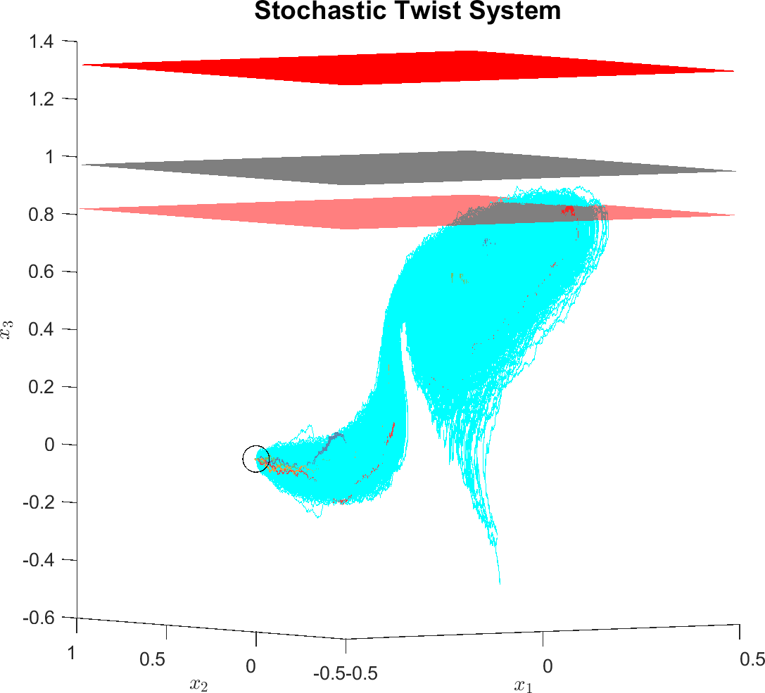
Figure 3: Trajectories of (49) with mean VP (solid red), mean ES (translucent black), and $\epsilon=0.15$ (translucent red) bounds

Table 6: Solver time (seconds) to compute Table 5

order	2	3	4	5	6
$\epsilon=0.5$	0.428	1.939	5.196	19.201	83.679
$\epsilon=0.15$	0.328	0.999	4.755	21.108	96.985
$\epsilon=0.1$	0.325	1.083	5.172	22.596	119.823
$\epsilon=0.05$	0.325	1.294	4.516	22.357	115.820

Table 7: ES Chance-Peak estimation of the Stochastic Twist System (49) to maximize $p(x)=x_{3}$

order	2	3	4	5	6	ES MC
mean	0.9100	0.8312	0.8231	0.8211	0.8203
$\epsilon=0.15$	1.4519	1.1251	1.0246	0.9892	0.9733	0.7923
$\epsilon=0.1$	1.5850	1.1880	1.0613	1.0173	0.9950	0.8016
$\epsilon=0.05$	1.8479	1.3063	1.1286	1.0646	1.0329	0.8156

Table 8: Solver time (seconds) to compute Table 7

order	2	3	4	5	6
mean	0.761	0.502	1.845	5.078	27.543
$\epsilon=0.15$	0.386	0.469	0.996	4.383	35.634
$\epsilon=0.1$	0.330	0.381	1.030	4.115	20.513
$\epsilon=0.05$	0.328	0.387	1.014	5.451	26.280

8.3 Discrete-time System

The prior examples involved SDE dynamics. In this subsection, we focus on a discrete-time system in which the parameter $\lambda\in\mathbb{R}$ is sampled according to the unit normal distribution at each time step ($\lambda[t]\sim\mathcal{N}(0,1)$). The discrete-time system system considered is

$$x_{+}=\begin{bmatrix}-0.3x_{1}+0.8x_{2}+x_{1}x_{2}\lambda/4\\ -0.9x_{1}--0.1x_{2}-0.2x_{1}^{2}+\lambda/40\end{bmatrix}.$$ (50)

This system involves a time horizon of $T=1$ with a time step of $\Delta t=1/10$ (10 iterations after the initial condition). The initial point is $x_{0}=[-1;0.5]$, and trajectories evolve in a support set of $X=[-1.5,1.5]^{2}$. Trajectories and order-6 bounds to maximize $p(x)=-x_{2}$ are displayed in Figure 4.

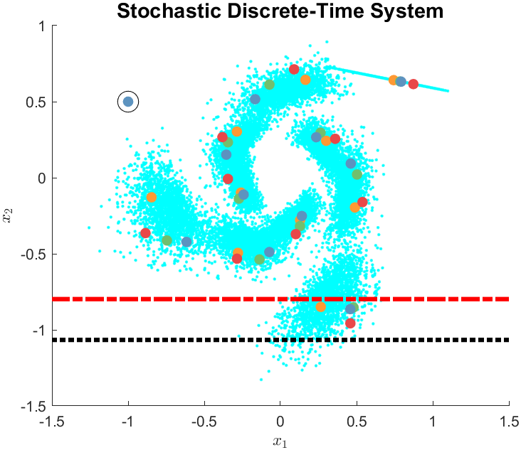
Figure 4: Trajectories of (50) with $\epsilon=\{0.5,\textrm{ES}\ 0.15\}$ bounds

Table 9 reports ES bounds for $-x_{2}$ at orders $1$ to $6$. The VP and Cantelli objectives produce bounds that are greater than $1.5$ (outside $X$) for the $d$ and $\epsilon$ values tested. As an example, the VP bound at $d=6,\epsilon=0.15$ is $p(x)\leq-2.1252$

Table 9: ES Chance-Peak estimation of the Discrete-time system (50) to maximize $p(x)=-x_{2}$

order	2	3	4	5	6	ES MC
mean	0.8766	0.8128	0.8002	0.7982	0.7976
$\epsilon=0.15$	1.5000	1.2139	1.0971	1.0743	1.0663	1.0287
$\epsilon=0.1$	1.5000	1.2973	1.1446	1.1083	1.0997	1.0601
$\epsilon=0.05$	1.5000	1.4500	1.2285	1.1653	1.1540	1.1092

8.4 Switching

We utilize a modification of Example C from [28] for this final example. The two subsystems involved are:

$$dx =\begin{bmatrix}-2.5x_{1}-2x_{2}\\ -0.5x_{1}-x_{2}\end{bmatrix}dt+\begin{bmatrix}0\\ 0.25x_{2}\end{bmatrix}dW$$ (51a)

$$dx =\begin{bmatrix}-x_{1}-2x_{2}\\ 2.5x_{1}-x_{2}\end{bmatrix}dt+\begin{bmatrix}0\\ 0.25x_{2}\end{bmatrix}dW.$$ (51b)

Switched SDE trajectories start from an initial condition of $X_{0}=(0,1)$ and are tracked in the state set $X=[-2,2]^{2}$ with a time horizon of $T=5$. The chance-peak problem is solved to find bounds on $p(x)=-x_{2}$.

Figure (5) plots switched SDE trajectories along with $\epsilon=\{0.5,\text{\acs{CVAR}}\ 0.15,\text{\acs{VP}}\ 0.15\}$ bounds (at order-6). Tables 10 and 12 list these discovered bounds.

Table 10: VP Chance-Peak upper-bounds for $p(x)=-x_{2}$ for the Switched System (51)

order	2	3	4	5	6	VaR MC
mean	0.4304	0.3823	0.3630	0.3487	0.3352	0.0788
$\epsilon=0.15$	0.9953	0.9328	0.9076	0.8918	0.8853	0.2384
$\epsilon=0.1$	1.2888	1.2162	1.1865	1.1687	1.1609	0.2755
$\epsilon=0.05$	1.9469	1.8516	1.8120	1.7891	1.7799	0.3334

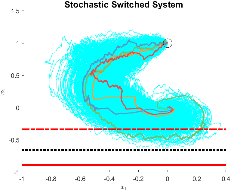
Figure 5: Trajectories of the switched system (51) with $\epsilon=\{0.5,\text{\acs{CVAR}}\ 0.15,\text{\acs{VP}}\ 0.15\}$ bounds

Table 11: Solver time (seconds) to compute Table 10

order	2	3	4	5	6
mean	0.362	0.389	0.570	1.755	2.499
$\epsilon=0.15$	0.257	0.295	0.587	1.812	3.718
$\epsilon=0.1$	0.237	0.281	1.636	2.364	3.191
$\epsilon=0.05$	0.251	0.291	0.906	1.735	2.638

Table 12: ES Chance-Peak upper-bounds for $p(x)=-x_{2}$ for the Switched System (51)

order	2	3	4	5	6	ES MC
mean	0.4304	0.3823	0.3630	0.3488	0.3350
$\epsilon=0.15$	0.9698	0.7882	0.7157	0.6803	0.6540	0.4220
$\epsilon=0.1$	1.1137	0.8818	0.7886	0.7433	0.7133	0.4470
$\epsilon=0.05$	1.3924	1.0548	0.9207	0.8585	0.8200	0.4688

Table 13: Solver time (seconds) to compute Table 10

order	2	3	4	5	6
mean	0.471	0.466	0.674	1.916	3.310
$\epsilon=0.15$	0.336	0.371	0.835	1.954	3.170
$\epsilon=0.1$	0.330	0.360	0.816	2.177	4.237
$\epsilon=0.05$	0.331	0.373	0.728	1.486	3.602

8.5 Distance Estimation

This example will involve distance estimation of a modification of the second subsystem of (51):

$$dx=\begin{bmatrix}-x_{1}-2x_{2}\\ 2.5x_{1}-x_{2}\end{bmatrix}dt+\begin{bmatrix}0\\ 0.1\end{bmatrix}dW.$$ (52)

This $L_{2}$ chance-distance task takes place at a time horizon of $T=5$ with sets $X_{0}=[0;0.75]$, $X=[-1.25,1]\times[-1,1]$, and $X_{u}=\{x_{u}\in\mathbb{R}^{2}\mid 0.1^{2}\geq(x_{u1}+1)^{2}+(x_{u2}+1)^{2},\ x_{u1}+x_{u2}\leq-2\}$. Distance estimation was accomplished by maximizing VaRs of the function $-\lVert x-x_{u}\rVert^{2}_{2}$ in (24), or by minimizing the ES distance program in (47).

System trajectories of (52) are displayed in Figure 6, in which the unsafe half-circle set $X_{u}$ is drawn in solid red. Squared distance lower bounds from solving SDPs arising from distance moment programs are listed in Table 14 and 16. Negative distance lower-bounds are truncated to $0$ in Table 14. This example demonstrates how the VP chance-peak distance bounds for distance estimation are very conservative, and how ES can offer an improvement in stochastic safety analysis.

Table 14: VP Chance-Peak squared distance lower bounds for System (52)

order	2	3	4	5	6	VAR MC
mean	1.1929	1.2337	1.2425	1.2490	1.2506	1.3162
$\epsilon=0.15$	0	0	0	0.0182	0.0235	1.2432
$\epsilon=0.1$	0	0	0	0	0	1.2261
$\epsilon=0.05$	0	0	0	0	0	1.2012

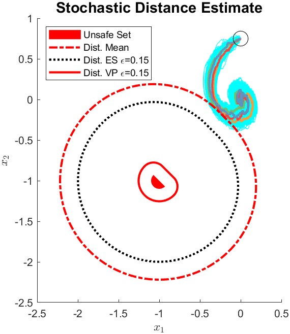
Figure 6: Trajectories of (52) with $\epsilon=\{0.5,0.15\}$ bounds

Table 15: Solver time (seconds) to compute Table 14

order	2	3	4	5	6
mean	0.507	0.512	1.772	6.569	21.331
$\epsilon=0.15$	0.346	0.453	1.233	5.836	23.930
$\epsilon=0.1$	0.344	0.482	1.522	5.172	21.034
$\epsilon=0.05$	0.384	0.485	1.711	5.954	26.974

Table 16: ES Chance-Peak squared distance lower bounds for System (52)

order	2	3	4	5	6	ES MC
mean	1.1929	1.2337	1.2427	1.2498	1.2494
$\epsilon=0.15$	0	0	0.4884	0.5061	0.7980	1.2079
$\epsilon=0.1$	0	0	0.2825	0.3018	0.7047	1.1942
$\epsilon=0.05$	0	0	0	0	0.4952	1.1734

Table 17: Solver time (seconds) to compute Table 16

order		2	3	4	5	6
mean	0.272	0.295	1.229	10.869	6.556
$\epsilon=0.15$	0.147	0.207	1.616	4.403	8.655
$\epsilon=0.1$	0.129	0.187	1.178	4.987	8.386
$\epsilon=0.05$	0.119	0.193	0.430	1.382	7.617

9 Conclusion

This paper considered the problem of finding the maximizing VaR of a state function $p(x)$ along trajectories of SDE systems. Two upper-bounding methods were used to approximate this maximum VaR: tail-bounds and ES. The tail-bounds are used to formulate an SOCP in measures (24), while ES produces an LP in measures (29). Each of these convex programs in measures are approximated by the moment-SOS hierarchy of SDPs in a convergent manner if the problem data (dynamics, support sets) is polynomial.

Future work avenue involves reducing the conservatism of chance-peak based distance estimation, developing stochastic optimal control strategies to minimize quantile statistics, and applying chance-peak techniques towards analysis of hybrid systems.

Appendix A Strong Duality of Measure SDPs

The work in [43] gives sufficient condition to ensure strong duality in the framework of linear programming on measures. This appendix generalizes the results of [43] by forming a framework of convex programming on measures with infinite-dimensional linear constraints and finite dimensional LMI constraints on moments. In particular, we add the case of optimization over Borel measures with SOC constraints on their moments to the original framework [43].

Let $M,m_{0}\in\mathbb{N}$ be positive integers. For $i=1..M$, let $m_{i}\in\mathbb{N}$ and $X_{i}\subset\mathbb{R}^{m_{i}}$ be a compact set. Let:

• $\mathcal{X}_{0}\subset\mathbb{S}^{m_{0}}$ be a vector space of symmetric matrices. Specific instances of $\mathcal{X}_{0}$ could be $\{\mathrm{diag}(\chi)\;|\;\chi\in\mathbb{R}^{m_{0}}\}$ (the space of diagonal matrices, corresponding to linear programming), or $\mathcal{X}_{0}=\mathbb{S}^{m_{0}}$ (the space of all symmetric matrices, corresponding to semidefinite programming). In particular, there exists such a space to represent second order cone programming [41]),

• $\mathcal{X}_{\infty}=\mathcal{M}(X_{1})\times\ldots\times\mathcal{M}(X_{M})$ be a vector space of signed Borel measures, equipped with its weak-$*$ topology, so that its topological dual is $\mathcal{X}^{*}_{\infty}=C(X_{1})\times\ldots\times C(X_{M})$,

• $\mathcal{X}=\mathcal{X}_{0}\times\mathcal{X}_{\infty}$ be our decision space, with topological dual $\mathcal{X}^{*}=\mathcal{X}_{0}\times\mathcal{X}_{\infty}^{*}$,

• A Banach space $\mathcal{Y}$ with dual $\mathcal{Y}^{*}$ that will represent our constraint space for equality constraints. In the context of the moment-SOS hierarchy, $\mathcal{Y}$ is chosen as a product space of smooth/polynomial functions defined on compact sets,

• $\mathcal{X}_{+}=\{(X,\mu_{1},\ldots,\mu_{M})\in\mathcal{X}\;|\;X\succeq 0,\quad\forall i=1..M,\mu_{i}\in\mathcal{M}_{+}(X_{i})\}$ and

• $\mathcal{X}^{*}_{+}=\{(Y,v_{1},\ldots,v_{M})\in\mathcal{X}^{*}\;|\;Y\succeq 0,\quad\forall i=1..M,v_{i}\geq 0\}$ be two convex cones.

For $\phi=(X,\mu_{1},\ldots,\mu_{M})\in\mathcal{X}$ and $\psi=(Y,v_{1},\ldots,v_{M})\in\mathcal{X}^{*}$, we define the duality

$$\langle\psi,\phi\rangle_{\mathcal{X}}=\textrm{Tr}(X\,Y)+\sum_{i=1}^{M}\int_{X_{i}}v_{i}(x_{i})d\mu_{i}(x_{i}).$$ (53)

Similarly, we denote by $\langle\cdot,\cdot\rangle_{\mathcal{Y}}$ the duality between elements of $\mathcal{Y}$ and $\mathcal{Y}^{*}$. Let $A:\mathcal{X}\longrightarrow\mathcal{Y}^{*}$ be a continuous linear map, $y\in\mathcal{Y}^{*}$ be a vector of continuous linear forms (when $\mathcal{Y}$ is made of polynomials, $y$ is a moment sequence), $C\in\mathcal{X}_{0}$, $p\in\mathbb{R}[x_{1}]\times\ldots\times\mathbb{R}[x_{M}]\subset\mathcal{X}^{*}_{\infty}$ be a vector of polynomials $\gamma=(C,g)\in\mathcal{X}^{*}$. We consider the following moment-SDP problem:

$$p^{*}_{M}= \sup\quad\langle\gamma,\phi\rangle_{\mathcal{X}}, \phi \in\mathcal{X}_{+}, A\phi =y$$ (54a)

with dual problem

$$d^{*}_{M}= \inf\quad\langle w,y\rangle_{\mathcal{Y}}, w \in\mathcal{Y}, A^{\dagger}w-\gamma \in\mathcal{X}^{*}_{+}.$$ (54b)

It is well known that weak duality $p^{*}_{M}\leq d^{*}_{M}$ always holds [49]. In this section, we will prove that under some mild assumptions, strong duality $p^{*}_{M}=d^{*}_{M}$ also holds.

We first prove a simple lemma on strong duality conditions.

Lemma A.1.

In this lemma, we consider again the duality pair (54), but with generic spaces $\mathcal{X}$, $\mathcal{Y}$ and a convex cone $\mathcal{X}_{+}$. We also define, for any vector space $\mathcal{Z}$ containing some vector $\eta$ and any linear map $U:\mathcal{X}\longrightarrow\mathcal{Z}$, the level set $U_{\eta}=\{\phi\in\mathcal{X}\;|\;U\phi=\eta\}$. In such setting, we assume that

1. $\exists\phi\in\mathcal{X}_{+}$ such that $A\phi=y$.

2. $A_{0}\cap\gamma_{0}\cap\mathcal{X}_{+}=\{0\}$.

3. $\exists\psi\in\mathcal{X}^{*}$ such that

   1. $\langle\psi,\mathcal{X}_{+}\rangle_{\mathcal{X}}\subset\mathbb{R}_{+}$

   2. $\psi_{0}\cap\mathcal{X}_{+}=\{0\}$

   3. $\psi_{1}\cap\mathcal{X}_{+}$ is compact.

Then, $p^{*}_{M}=d^{*}_{M}.$

Moreover, if $p^{*}_{M}<\infty$, then there is an optimal $\phi^{*}$ feasible for (54a) such that $\langle\gamma,\phi^{*}\rangle_{\mathcal{X}}=p^{*}_{M}$.

Proof.

We use [49, Chap. IV: Thm (7.2), Lem (7.3)]. Consider the cone

$$\mathcal{X}_{A}^{\gamma}=\{(A\phi,\langle\gamma,\phi\rangle_{\mathcal{X}})\;|\;\phi\in\mathcal{X}_{+}\}.$$

Theorem (7.2) of [49] ensures that under A1’ and closedness of $\mathcal{X}_{A}^{\gamma}$, strong duality holds, and that $p^{*}_{M}<\infty$ then implies existence of an optimal $\phi^{*}$. Then, Lemma (7.3) of [49] states that if $\mathcal{X}_{+}$ has a compact convex base and A2’ holds, then $A_{\mathcal{X}}^{\gamma}$ is closed. Thus, we need to find a compact convex base of $\mathcal{X}_{+}$.

Let $\phi\in\mathcal{X}_{+}\setminus\{0\}$. A3’.(a)-(b) ensure that $\langle\psi,\phi\rangle_{\mathcal{X}}>0$ so that $\tilde{\phi}=\frac{\phi}{\langle\psi,\phi\rangle_{\mathcal{X}}}$ is well defined and belongs to the cone $\mathcal{X}_{+}\setminus\{0\}$. Moreover, $\langle\psi,\tilde{\phi}\rangle_{\mathcal{X}}=1$ is clear by definition, so that $\tilde{\phi}\in\psi_{1}\cap\mathcal{X}_{+}$. This proves that any $\phi\in\mathcal{X}_{+}\setminus\{0\}$ can be described as $\phi=\langle\psi,\phi\rangle_{\mathcal{X}}\tilde{\phi}$ with $\tilde{\phi}\in\psi_{1}\cap\mathcal{X}_{+}$ and $\langle\psi,\phi\rangle_{\mathcal{X}}>0$, which is the definition of $\psi_{1}\cap\mathcal{X}_{+}$ being a base of $\mathcal{X}$. By compactness assumption A3’.(c), we deduce that the assumptions of Lemma (7.3) of Theorem (7.2) of [49] hold: $X_{A}^{\gamma}$ is closed and thus $p^{*}_{M}=d^{*}_{M}$. ∎

Theorem A.2.

Suppose that there exists $B>0$ such that for all $\phi=(X,\mu_{1},\ldots,\mu_{M})$ feasible for (54a), one has $\textrm{Tr}(X^{2})\leq B^{2}$ and for $i=1..M$, $\langle 1,\mu_{i}\rangle\leq B$. Also assume that at least one such feasible $\phi$ exists. Then, $p^{*}_{M}=d^{*}_{M}$. Moreover, there exists an optimal $\phi^{*}$ such that $A\phi^{*}=y$ and $\langle\gamma,\phi^{*}\rangle_{\mathcal{X}}=p^{*}_{M}$.

Proof.

We prove that the assumptions of Lemma A.1 hold. First of all, $\mathcal{X}_{+}$ is indeed a convex cone under A1’, as it is the product of convex cones $\mathbb{S}_{+}^{m_{0}}$ and $\mathcal{M}_{+}(X_{i})$.

Next, we focus on hypothesis A2’ Let $\phi=(X,\mu_{1},\ldots,\mu_{M})\in A_{0}\cap\gamma_{0}\cap\mathcal{X}_{+}$. We want to prove that $\phi=0$. Let $\phi^{(0)}=(X^{(0)},\mu_{1}^{(0)},\ldots,\mu_{M}^{(0)})\in\mathcal{X}_{+}$ such that $A\phi^{(0)}=y$. Define, for $t\geq 0$, $\phi^{(t)}=\phi^{(0)}+t\phi$. Let $t\geq 0$. Since $\mathcal{X}_{+}$ is a convex cone, $\phi^{(t)}\in\mathcal{X}_{+}$. In addition,

$$A\phi^{(t)}=A\phi^{(0)}+t\,A\phi=A\phi^{(0)}=y,$$

so that $\phi^{(t)}$ is feasible for (54a). Thus, by assumption,

$$B^{2} \geq\textrm{Tr}((X^{(0)}+tX)^{2})$$

$$=\textrm{Tr}(X^{(0)2}+2tX^{(0)}X+t^{2}X^{2})$$

$$=\textrm{Tr}(X^{(0)2})+2t\textrm{Tr}(X^{(0)}X)+t^{2}\textrm{Tr}(X^{2})$$

$$=t^{2}\textrm{Tr}(X^{2})+\underset{t\to\infty}{o}(t^{2}).$$

Staying bounded when $t$ goes to infinity requires that $\textrm{Tr}(X^{2})=0$, implying that $X=0$. The same reasoning replacing $\textrm{Tr}(X^{2})$ with $\langle 1,\mu_{i}\rangle$ yields that for all $i=1..M$, $\mu_{i}=0$. Thus, $\phi=0$ and A2’ holds.

We turn to A3’ and consider $\psi=(I_{m_{0}},1_{M})$ where $I_{m_{0}}$ is the size $m_{0}$ identity matrix and $1_{M}$ is the dimension $M$ vector of functions that are all constant equal to $1$. Note that if $(X,\mu_{1},\ldots,\mu_{M})\in\mathcal{X}_{+}$, then $\textrm{Tr}(X)\geq 0$ and $\forall i=1..M:\ \langle 1,\mu_{i}\rangle\geq 0$ (i.e. $\langle\psi,\mathcal{X}_{+}\rangle_{\mathcal{X}}\subset\mathbb{R}_{+}$). Moreover the equality cases in those inequalities only hold for $X=0$ and $\mu_{i}=0$ respectively, so that $\psi_{0}\cap\mathcal{X}_{+}=\{0\}.$ It only remains to prove that $\psi_{1}\cap\mathcal{X}_{+}$ is compact.

First, it is bounded for the norm $\lVert(X,\mu_{1},\ldots,\mu_{M})\rVert=\sqrt{\textrm{Tr}(X^{2})}+\sum_{i=1}^{M}\lVert\mu_{i}\rVert_{TV}$ where the total variation norm of a signed measure is

$$\lVert\mu\rVert_{TV}=\sup\{\langle v,\mu\rangle\;|\;-1\leq v\leq 1\}.$$

In particular, the total variation norm of a nonnegative measure $\mu\in\mathcal{M}_{+}(X)$ is equal to its mass $\lVert\mu\rVert_{TV}=\langle 1,\mu\rangle$.

Indeed, let $(X,\mu_{1},\ldots,\mu_{M})\in\psi_{1}\cap\mathcal{X}_{+}$; then $\textrm{Tr}(X)\leq 1$ and for $i=1..M$, $1\geq\langle 1,\mu_{i}\rangle=\lVert\mu_{i}\rVert_{TV}$. As $X$ is positive semidefinite, $\textrm{Tr}(X)\leq 1$ means that none of the eigenvalues of $X$ are bigger than $1$. As such, $\textrm{Tr}(X^{2})\leq m_{0}$, because it is the sum of the squares of the eigenvalues of $X$. Thus, for all $\phi\in\psi_{1}\cap\mathcal{X}_{+}$, $\lVert\phi\rVert\leq m_{0}+M$.

Then, it is also closed for the weak-* topology of $\mathcal{X}$ by continuity of $\langle\psi,\cdot\rangle_{\mathcal{X}}$ and closedness of $\mathcal{X}_{+}$ as the product of closed sets $\mathbb{S}^{m_{0}}_{+}$ and $\mathcal{M}_{+}(X_{i})$. Thus, $\psi_{1}\cap\mathcal{X}_{+}$ is weak-* closed and bounded: according to the Banach-Alaoglu theorem, it is compact: assumption A3’ of Lemma A.1 holds, which concludes the proof of strong duality.

Finally, let $\phi=(X,\mu_{1},\ldots,\mu_{M})\in\mathcal{X}_{+}$ feasible for (54a). Then, by assumption, $\textrm{Tr}(X^{2})\leq B^{2}$ and $\langle 1,\mu_{i}\rangle\leq B$ for all $i=1..M$. Thus, one has

$$\langle\gamma,\phi\rangle_{\mathcal{X}} =\textrm{Tr}(C\,X)+\sum_{i=1}^{M}\langle g_{i},\mu_{i}\rangle.$$

Using the Cauchy-Schwarz inequality results in

$$\leq\sqrt{\textrm{Tr}(C^{2})\textrm{Tr}(X^{2})}+\sum_{i=1}^{M}\langle g_{i},\mu_{i}\rangle$$

$$\leq\sqrt{\textrm{Tr}(C^{2})\textrm{Tr}(X^{2})}+\sum_{i=1}^{M}\sup_{X_{i}}|g_{i}|\langle 1,\mu_{i}\rangle$$

$$\leq\left(\sqrt{\textrm{Tr}(C^{2})}+\sum_{i=1}^{M}\lVert g_{i}\rVert_{\infty}\right)B$$

so that taking the supremum over all feasible $\phi$ yields

$$p^{*}_{M}\leq\left(\sqrt{\textrm{Tr}(C^{2})}+\sum_{i=1}^{M}\lVert g_{i}\rVert_{\infty}\right)B<\infty,$$

which is the last hypothesis of Lemma A.1 and ensures existence of an optimal solution. ∎

Appendix B Strong Duality of Chance-Peak Concentration-Bound Linear Programs

In order to apply the strong duality results of Appendix A towards the tail-bound chance-peak problem (Theorem 4.7), we need to provide an SDP-representation of the SOC cone.

Lemma B.1.

An element $(y,s)\in\mathbb{L}^{n}$ satisfies the LMI [41]

$$\Phi=\begin{bmatrix}s&y^{T}\\ y&sI_{n}\end{bmatrix}\succeq 0.$$ (55)

Proof.

When ${s}=0$, the containment $({y},0)\in{\mathbb{L}}^{n}$ requires that ${y}=\mathbf{0}_{n}$. The matrix in $\Phi$ (55) is therefore the $\mathbf{0}_{n\times n}$ matrix which is PSD. Now consider the case where ${s}>0$. A Schur complement of $\Phi$ yields the constraint ${s-y^{T}y/s}\geq 0$. Multiplying through by the positive ${s}$ results in ${s^{2}-\lVert y\rVert^{2}_{2}}\geq 0,\ {s}>0$, which is the definition of the SOC cone ${(y,s)\in\mathbb{L}^{n}}$. Lemma B.1 is therefore proven. ∎

Lemma B.1 ensures that problem (25) is an instance of the more generic (54a) with $M=2$, $X_{1}=X_{2}=[0,T]\times X$, $\mathcal{Y}=C^{2}([0,T]\times X)\times\mathbb{R}^{3}$ and

$$\mathcal{X}_{0}=\left\{{\begin{bmatrix}s&y^{T}\\ y&sI_{3}\end{bmatrix}}\;\middle|\;{s\in\mathbb{R},y\in\mathbb{R}^{3}}\right\}.$$ (56)

Therefore, we only need to verify that the hypotheses of Theorem A.2 hold in our specific case.

Letting ${z}=([{z}_{1},{z}_{2},{z}_{3}],{z}_{4})\in\mathbb{L}^{3}$ be an SOC-constrained variable, we define the matrix $\Phi$ from (55) as

$$\Phi=\begin{bmatrix}{z}_{4}&{z}_{1}&{z}_{2}&{z}_{3}\\ {z}_{1}&{z}_{4}&0&0\\ {z}_{2}&0&{z}_{4}&0\\ {z}_{3}&0&0&{z}_{4}\end{bmatrix}.$$ (57)

Theorem A.2 requires the following sufficient conditions to prove strong duality between (25) and (26) and their optimality obtainment.

1. There exists a feasible solution for $(\mu_{\tau},\mu,{z})$ from (25).

2. The measures $\mu_{\tau},\mu$ are bounded.

3. The square of the matrix $\Phi$ from (57) has bounded trace.

We start with R1. Letting $x(t\mid x_{0})$ be an SDE trajectory from (11) and $t^{*}\in(0,T]$ be a stopping time with $\tau^{*}=t^{*}\wedge\tau_{X}$, we define $\mu$ as the occupation measure of $x(t\mid x_{0})$ and $\mu_{\tau}$ as its time-$\tau^{*}$ state distribution $\mu_{\tau^{*}}$. Feasible choices for entries of the SOC-constrained ${z}$ are (from Lemma 4.4)

$${z}_{1} =1-\langle p^{2},\mu_{t^{*}}\rangle, {z}_{2} =\sqrt{\langle p^{2},\mu_{t^{*}}\rangle-\langle p,\mu_{t^{*}}\rangle^{2}},$$ (58)

$${z}_{3} =2\langle p,\mu_{t^{*}}\rangle, {z}_{4} =1+\langle p^{2},\mu_{t^{*}}\rangle.$$ (59)

Requirement R2’s satisfaction follows the statement in Lemma 6.2 that $\mu_{\tau},\mu$ are bounded under A1-A3.

We end with R3. The trace $\textrm{Tr}(\Phi^{2})=\sum_{ij}\Phi_{ij}^{2}$ is equal to

$$\textrm{Tr}(\Phi^{2}) =2{z}_{1}^{2}+2{z}_{2}^{2}+2{z}_{3}^{2}+4{z}_{4}^{2}$$ (60a)

$$=2(1-\langle p^{2},\mu_{t^{*}}\rangle)^{2}+2(\sqrt{\langle p^{2},\mu_{t^{*}}\rangle-\langle p,\mu_{t^{*}}\rangle^{2}})^{2}$$

$$\qquad+2(2\langle p,\mu_{t^{*}}\rangle)^{2}+4(1+\langle p^{2},\mu_{t^{*}}\rangle)^{2}$$ (60b)

$$=6+6\langle p,\mu_{t^{*}}\rangle^{2}+6\langle p^{2},\mu_{t^{*}}\rangle+6\langle p^{2},\mu_{t^{*}}\rangle^{2}.$$ (60c)

Let $\Pi_{1}=\max_{x\in X}p(x)$ and $\Pi_{2}=\max_{x\in X}p(x)^{2}$ be bounds on $p$ and $p^{2}$ in $X$. Both $\Pi_{1}$ and $\Pi_{2}$ will be finite by the compactness of $X$ (A1) and the continuity of $p$ within $X$ (A3). Given that $\mu_{t^{*}}$ is a probability distribution supported in $X$, the moments of $\mu_{t^{*}}$ will be bounded by $\langle p,\mu_{t^{*}}\rangle\leq\Pi_{1}$ and $\langle p^{2},\mu_{t^{*}}\rangle\leq\Pi_{2}$. The squared-trace in (60) can be upper-bounded by a finite value $B^{2}$ such that

$$\textrm{Tr}(\Phi^{2})\leq 6(1+\Pi_{1}^{2}+\Pi_{2}+\Pi_{2}^{2})=B^{2}<\infty.$$ (61)

The finite bound $B^{2}\in[0,\infty)$ from (61) validates R3, and completes all conditions necessary for Theorem A.2 to provide for strong duality and optima attainment.

Appendix C Strong Duality of Chance-Peak Expected Shortfall Linear Programs

We follow the steps and conventions of Theorem 2.6 of [50] to perform this proof of strong duality.

We collect the groups of variables into

$$\boldsymbol{\mu} =(\mu_{\tau},\mu,{\nu,\hat{\nu}}) \boldsymbol{\ell} =({u,v,w}).$$ (62)

We now define the following variable spaces

$$\mathcal{X}^{\prime} =C([0,T]\times X)^{2}\times C(\mathbb{R})^{2}$$ (63)

$$\mathcal{X} =\mathcal{M}([0,T]\times X)^{2}\times\mathcal{M}(\mathbb{R})^{2},$$

and note that their nonnegative subcones are

$$\mathcal{X}_{+}^{\prime} =C_{+}([0,T]\times X)^{2}\times C_{+}(\mathbb{R})^{2}$$ (64)

$$\mathcal{X}_{+} =\mathcal{M}_{+}([0,T]\times X)^{2}\times\mathcal{M}_{+}(\mathbb{R})^{2}.$$

Additionally, the measure $\boldsymbol{\mu}$ from (62) obeys $\boldsymbol{\mu}\in\mathcal{X}_{+}$. Assumption A1 imposes that the cones $\mathcal{X}_{+}^{\prime}$ and $\mathcal{X}_{+}$ in (64) form a pair of topological duals.

We define the constraint spaces $\mathcal{Y}$ and $\mathcal{Y}^{\prime}$ as

$$\mathcal{Y}^{\prime} ={\mathbb{R}\times\mathcal{C}([0,T]\times X)\times C(\mathbb{R})}$$ (65)

$$\mathcal{Y} ={0\times\mathcal{C}([0,T]\times X)^{\prime}\times\mathcal{M}(X)}.$$ (66)

We follow the convention of [50] and define $\mathcal{Y}_{+}={\{0_{\mathcal{Y}}\}}$ and $\mathcal{Y}^{\prime}_{+}=\mathcal{Y}^{\prime}$. The variable $\boldsymbol{\ell}$ from 62 satisfies $\boldsymbol{\ell}\in\mathcal{Y}^{\prime}$.

We formulate the affine maps of

$$\mathcal{A}(\boldsymbol{\mu}) =[{\langle 1,\nu\rangle},\ \mu_{\tau}-\mathcal{L}^{\dagger}\mu,\ \epsilon{\nu+\hat{\nu}}-p_{\#}\mu_{\tau}]$$ (67)

$$\mathcal{A}^{*}(\boldsymbol{\ell}) =[{v-w\circ p,\ -\mathcal{L}v,\ u+\epsilon w,\ w}],$$

and the associated cost/constraint data

$$\mathbf{b} =[1,\ \delta_{0}\otimes\mu_{0},\ 0] \mathbf{c} =[0,\ 0,\ {\mathrm{id}_{\mathbb{R}}},\ 0].$$ (68a)

We point out that $\mathcal{A}$ and $\mathcal{A}^{*}$ are linear adjoints, that $\mathcal{X}$ has a weak-* topology, and that $\mathcal{Y}$ has a sup-norm-bounded weak topology. We also note that the following pairings satisfy

$$\langle\mathbf{c},\boldsymbol{\mu}\rangle =\langle\mathrm{id}_{\mathbb{R}},\nu\rangle$$ (69a)

$$\langle\boldsymbol{\ell},\mathbf{b}\rangle ={u}+\langle v(0,{\bullet}),\mu_{0}\rangle.$$ (69b)

Problem (29) may be expressed as

$$p^{*}= \sup_{\boldsymbol{\mu}\in\mathcal{X}_{+}}\langle\mathbf{c},\boldsymbol{\mu}\rangle \mathbf{b}-\mathcal{A}(\boldsymbol{\mu})\in\mathcal{Y}_{+}.$$ (70)

Problem (30) may be converted into

$$d^{*}= \inf_{\boldsymbol{\ell}\in\mathcal{Y}^{\prime}_{+}}\langle\boldsymbol{\ell},\mathbf{b}\rangle \mathcal{A}^{\prime}(\boldsymbol{\ell})-\mathbf{c}\in\mathcal{X}_{+}.$$ (71)

Sufficient conditions for strong duality from [50, Theorem 2.6] are:

• Masses of measures in $\boldsymbol{\mu}$ satisfying $b-\mathcal{A}(\boldsymbol{\mu})\in\mathcal{Y}_{+}$ are bounded.

• There exists a feasible $\boldsymbol{\mu}^{f}$ with $b-\mathcal{A}(\boldsymbol{\mu}^{f})\in\mathcal{Y}_{+}$.

• Functions involved in defining $\mathbf{c}$, $\mathbf{b}$, and $\mathcal{A}$ are continuous.

Requirement R1 is satisfied by Theorem 6.5 under A1, A3, and A4. Requirement R2 holds because there exists a feasible solution $\boldsymbol{\mu}^{f}$ from the proof of Theorem 5.4 (constructed from a feasible trajectory of the stochastic process) under A4. Requirement R3 is fulfilled because $v\in\mathcal{C}([0,T]\times X)$ implies that $\mathcal{L}v\in C([0,T]\times X)$ (A2) and $p$ is continuous (A3). All requirements are fulfilled, which proves strong duality between (29) and (30).

References

- [1] P. Jorion, Value at Risk. McGraw-Hill Professional Publishing, 2000.
- [2] F. P. Cantelli, “Sui confini della probabilita,” in Atti del Congresso Internazionale dei Matematici: Bologna del 3 al 10 de settembre di 1928, 1929, pp. 47–60.
- [3] D. Vysochanskij and Y. I. Petunin, “Justification of the 3 rule for unimodal distributions,” Theory of Probability and Mathematical Statistics, vol. 21, no. 25-36, 1980.
- [4] J. Dupačová, “The minimax approach to stochastic programming and an illustrative application,” Stochastics, vol. 20, no. 1, pp. 73–88, 1987.
- [5] G. C. Pflug, “Some Remarks on the Value-at-Risk and the Conditional Value-at-Risk,” in Probabilistic constrained optimization. Springer, 2000, pp. 272–281.
- [6] R. T. Rockafellar and S. Uryasev, “Conditional Value-at-Risk for General Loss Distributions,” Journal of banking & finance, vol. 26, no. 7, pp. 1443–1471, 2002.
- [7] P. Artzner, F. Delbaen, J.-M. Eber, and D. Heath, “Coherent measures of risk,” Mathematical finance, vol. 9, no. 3, pp. 203–228, 1999.
- [8] S. Sarykalin, G. Serraino, and S. Uryasev, “Value-at-risk vs. conditional value-at-risk in risk management and optimization,” in State-of-the-art decision-making tools in the information-intensive age. Informs, 2008, pp. 270–294.
- [9] A. Wang, A. Jasour, and B. C. Williams, “Non-gaussian chance-constrained trajectory planning for autonomous vehicles under agent uncertainty,” IEEE Robotics and Automation Letters, vol. 5, no. 4, pp. 6041–6048, 2020.
- [10] W. Han, A. Jasour, and B. Williams, “Non-gaussian risk bounded trajectory optimization for stochastic nonlinear systems in uncertain environments,” in 2022 International Conference on Robotics and Automation (ICRA). IEEE, 2022, pp. 11 044–11 050.
- [11] C. W. Miller and I. Yang, “Optimal control of conditional value-at-risk in continuous time,” SIAM Journal on Control and Optimization, vol. 55, no. 2, pp. 856–884, 2017.
- [12] M. P. Chapman, R. Bonalli, K. M. Smith, I. Yang, M. Pavone, and C. J. Tomlin, “Risk-sensitive safety analysis using conditional value-at-risk,” IEEE Transactions on Automatic Control, vol. 67, no. 12, pp. 6521–6536, 2021.
- [13] A. Shapiro, D. Dentcheva, and A. Ruszczynski, Lectures on stochastic programming: modeling and theory. SIAM, 2021.
- [14] A. Ben-Tal, L. El Ghaoui, and A. Nemirovski, Robust Optimization. Princeton University Press, 2009, vol. 28.
- [15] G. Calafiore and M. C. Campi, “Uncertain convex programs: randomized solutions and confidence levels,” Mathematical Programming, vol. 102, no. 1, pp. 25–46, 2005.
- [16] M. C. Campi and S. Garatti, “A sampling-and-discarding approach to chance-constrained optimization: feasibility and optimality,” Journal of optimization theory and applications, vol. 148, no. 2, pp. 257–280, 2011.
- [17] R. Tempo, G. Calafiore, F. Dabbene et al., Randomized algorithms for analysis and control of uncertain systems: with applications. Springer, 2013, vol. 7.
- [18] C. M. Lagoa, X. Li, and M. Sznaier, “Probabilistically Constrained Linear Programs and Risk-Adjusted Controller Design,” SIAM Journal on Optimization, vol. 15, no. 3, pp. 938–951, 2005.
- [19] R. Lewis and R. Vinter, “Relaxation of Optimal Control Problems to Equivalent Convex Programs,” Journal of Mathematical Analysis and Applications, vol. 74, no. 2, pp. 475–493, 1980.
- [20] M. J. Cho and R. H. Stockbridge, “Linear Programming Formulation for Optimal Stopping Problems,” SIAM J. Control Optim., vol. 40, no. 6, pp. 1965–1982, 2002.
- [21] J. B. Lasserre, Moments, Positive Polynomials And Their Applications, ser. Imperial College Press Optimization Series. World Scientific Publishing Company, 2009.
- [22] J. B. Lasserre, D. Henrion, C. Prieur, and E. Trélat, “Nonlinear optimal control via occupation measures and lmi-relaxations,” SIAM journal on control and optimization, vol. 47, no. 4, pp. 1643–1666, 2008.
- [23] D. Henrion and M. Korda, “Convex computation of the region of attraction of polynomial control systems,” IEEE Transactions on Automatic Control, vol. 59, no. 2, pp. 297–312, 2013.
- [24] G. Fantuzzi and D. Goluskin, “Bounding Extreme Events in Nonlinear Dynamics Using Convex Optimization,” SIAM Journal on Applied Dynamical Systems, vol. 19, no. 3, pp. 1823–1864, 2020.
- [25] J. Miller, D. Henrion, M. Sznaier, and M. Korda, “Peak Estimation for Uncertain and Switched Systems,” in 2021 60th IEEE Conference on Decision and Control (CDC), 2021, pp. 3222–3228.
- [26] J.-B. Lasserre, T. Prieto-Rumeau, and M. Zervos, “Pricing a class of exotic options via moments and SDP relaxations,” Mathematical Finance, vol. 16, no. 3, pp. 469–494, 2006.
- [27] S. Prajna, A. Jadbabaie, and G. J. Pappas, “Stochastic safety verification using barrier certificates,” in 2004 43rd IEEE conference on decision and control (CDC)(IEEE Cat. No. 04CH37601), vol. 1. IEEE, 2004, pp. 929–934.
- [28] ——, “A Framework for Worst-Case and Stochastic Safety Verification Using Barrier Certificates,” IEEE Transactions on Automatic Control, vol. 52, no. 8, pp. 1415–1428, 2007.
- [29] K. Kashima and R. Kawai, “An optimization approach to weak approximation of Lévy-driven stochastic differential equations,” in Perspectives in Mathematical System Theory, Control, and Signal Processing. Springer, 2010, pp. 263–272.
- [30] G. Fantuzzi, D. Goluskin, D. Huang, and S. I. Chernyshenko, “Bounds for Deterministic and Stochastic Dynamical Systems using Sum-of-Squares Optimization,” SIAM Journal on Applied Dynamical Systems, vol. 15, no. 4, pp. 1962–1988, 2016.
- [31] B. Xue, N. Zhan, and M. Fränzle, “Reach-Avoid Analysis for Stochastic Differential Equations,” 2022.
- [32] A. M. Jasour, N. S. Aybat, and C. M. Lagoa, “Semidefinite Programming For Chance Constrained Optimization Over Semialgebraic Sets,” SIAM Journal on Optimization, vol. 25, no. 3, pp. 1411–1440, 2015.
- [33] E. de Klerk, D. Kuhn, and K. Postek, “Distributionally robust optimization with polynomial densities: theory, models and algorithms,” Mathematical Programming, vol. 181, pp. 265–296, 2020.
- [34] R. Tian, S. H. Cox, and L. F. Zuluaga, “Moment problem and its applications to risk assessment,” North American Actuarial Journal, vol. 21, no. 2, pp. 242–266, 2017.
- [35] J. Čerbáková, “Worst-case var and cvar,” in Operations Research Proceedings 2005: Selected Papers of the Annual International Conference of the German Operations Research Society (GOR), Bremen, September 7–9, 2005. Springer, 2006, pp. 817–822.
- [36] J. Miller, M. Tacchi, M. Sznaier, and A. Jasour, “Peak Value-at-Risk Estimation for Stochastic Differential Equations using Occupation Measures,” in 62nd IEEE Conference on Decision and Control, 2023.
- [37] H. Föllmer and A. Schied, “Convex and coherent risk measures,” Encyclopedia of Quantitative Finance, pp. 355–363, 2010.
- [38] B. Øksendal, “Stochastic Differential Equations: An Introduction with Applications ,” in Stochastic differential equations. Springer, 2003, pp. 65–84.
- [39] L. C. Rogers and D. Williams, Diffusions, Markov Processes, and Martingales. Cambridge university press, 2000, vol. 1.
- [40] E. B. Dynkin, “Markov Processes,” in Markov processes. Springer, 1965, pp. 77–104.
- [41] F. Alizadeh and D. Goldfarb, “Second-order cone programming,” Mathematical programming, vol. 95, no. 1, pp. 3–51, 2003.
- [42] J. Lofberg. (2009) Working with square roots. [Online]. Available: https://yalmip.github.io/squareroots
- [43] M. Tacchi, “Convergence of Lasserre’s hierarchy: the general case,” Optimization Letters, vol. 16, no. 3, pp. 1015–1033, 2022.
- [44] M. ApS, The MOSEK optimization toolbox for MATLAB manual. Version 9.2., 2020. [Online]. Available: https://docs.mosek.com/9.2/toolbox/index.html
- [45] J. Miller and M. Sznaier, “Bounding the Distance of Closest Approach to Unsafe Sets with Occupation Measures,” in 2022 61st IEEE Conference on Decision and Control (CDC), 2022.
- [46] ——, “Bounding the Distance to Unsafe Sets with Convex Optimization,” IEEE Transactions on Automatic Control, pp. 1–15, 2023.
- [47] H. Waki, S. Kim, M. Kojima, and M. Muramatsu, “Sums of Squares and Semidefinite Programming Relaxations for Polynomial Optimization Problems with Structured Sparsity,” SIOPT, vol. 17, no. 1, pp. 218–242, 2006.
- [48] J. Lofberg, “YALMIP : a toolbox for modeling and optimization in MATLAB,” in ICRA (IEEE Cat. No.04CH37508), 2004, pp. 284–289.
- [49] A. Barvinok, A Course in Convexity. American Mathematical Society, 2002.
- [50] M. Tacchi, “Moment-SOS hierarchy for large scale set approximation. Application to power systems transient stability analysis,” Ph.D. dissertation, Toulouse, INSA, 2021.