Energy-second-moment map analysis as an approach to quantify the irregularity
of Hamiltonian systems

Abstract

A different approach will be presented that aims to scrutinize the phase-space trajectories of a general class of Hamiltonian systems with regard to their regular or irregular behavior. The approach is based on the ‘energy-second-moment map’ that can be constructed for all Hamiltonian systems of the generic form $H=\bm{p}^{2}/2+V(\bm{q},t)$. With a three-component vector $\bm{s}$ consisting of the system’s energy $h$ and second moments $\bm{q}\bm{p}$, $\bm{q}^{2}$, this map linearly relates the vector $\bm{s}(t)$ at time $t$ with the vector’s initial state $\bm{s}(0)$ at $t=0$. It will turn out that this map is directly obtained from the solution of a linear third-order equation that establishes an extension of the set of canonical equations. The Lyapunov functions of the energy-second-moment map will be shown to have simple analytical representations in terms of the solutions of this linear third-order equation. Applying Lyapunov’s regularity analysis for linear systems, we will show that the Lyapunov functions of the energy-second-moment map yields information on the irregularity of the particular phase-space trajectory. Our results will be illustrated by means of numerical examples.

I Introduction

The phase-space trajectories of dynamical systems can be classified as being either regular or irregular. The distinction between regular and irregular behavior of a trajectory of a given $n$-degree-of-freedom dynamical system is commonly made on the basis of the linear system of perturbation equations that can be solved in conjunction with the full set of equations of motion. The $n\times n$ solution matrix of the system of perturbation equations is referred to as the stability matrix. This matrix thus describes the stability of all trajectories with respect to small changes of their initial values. From the stability matrix, the system’s degree of irregularity can then be quantified in terms of Lyapunov’s characteristic exponents (cf., for example, Refs. lyapu ; mayer ; ryabov ). The “degree of irregularity” of a given dynamical system is then defined as the proportion of the phase-space volume at $t=0$ that gives rise to irregular trajectories to the corresponding phase-space volume that leads to regular trajectories.

In this paper, a different approach to quantify the irregularity of the time evolution of dynamical systems will be presented. It applies to all—possibly explicitly time-dependent—Hamiltonian systems that are canonically equivalent to the generic Hamiltonian $H(\bm{q},\bm{p},t)=\bm{p}^{2}/2+V(\bm{q},t)$.

In contrast to conventional approaches that analyze the stability matrix, our method is based on the analysis of the “energy-second-moment map”struck . A derivation of this map will be sketched in Sec. II. Briefly, the energy-second-moment map linearly relates the three-component vector $\bm{s}(t)$ of system quantities energy $h$ and second moments $\bm{q}\bm{p}$, $\bm{q}^{2}$ at finite times $t$ with the vector’s initial state $\bm{s}(0)$ at $t=0$. Similar to the stability matrix, the energy-second-moment map is obtained by solving an additional set of linear differential equations on the top of the set of equations of motion. It will turn out that this map can be represented by a $3\times 3$ order matrix $\Xi(t)$ with unit determinant. As Lyapunov’s theory of characteristic coefficients can be applied to any linear system with time-dependent and generally nonperiodic coefficients, we may therefore make use of this theory to analyze the regularity of the energy-second-moment map.

We will give in Sec. III.1 a brief review of the Lyapunov regularity analysis of nonautonomous, homogeneous linear systems. Applied to the particular energy-second-moment matrix $\Xi(t)$, we will show in Sec. III.2 by means of a $QR$ decomposition of $\Xi(t)$ that its three Lyapunov functions $\lambda_{1,2,3}(t)$ always have a simple analytical representation in terms of the column vectors of $\Xi(t)$. Furthermore, we will see in Sec. III.3 that our analysis becomes particularly simple for autonomous (time-independent) Hamiltonian systems. On the basis of this astonishing result, we can easily determine the Lyapunov coefficient of irregularity of the energy-second-moment map and thereby quantify the system’s degree of irregularity. The regularity analysis emerging from the energy-second-moment map therefore simplifies the conventional approach that is based on the analysis of the stability matrix.

By means of several numerical examples, given in Sec. IV, we will illustrate that the degree of irregularity of a Hamiltonian system can indeed be quantified in terms of the time evolution of the Lyapunov coefficients $\lambda_{1,2,3}(t)$ of the energy-second-moment map. We will furthermore show that the time evolution of the Lyapunov functions of a chaotic trajectory allows to identify particular time intervals where the particle’s motion is quasi-regular.

II Energy-second-moment map

We consider an $n$-degree-of-freedom system of classical particles in a $2n$-dimensional Cartesian phase space whose Hamiltonian can be converted into the generic form

$$H(\bm{q},\bm{p},t)=\textstyle\frac{1}{2}\bm{p}^{2}+V(\bm{q},t).$$ (1)

Herein, $\bm{q}$ denotes the $n$-dimensional vector of configuration space variables, and $\bm{p}$ is the vector of conjugate momenta. The system’s time evolution is then given as the solutions of the canonical equations

$$\dot{\bm{q}}=\bm{p}\,,\qquad\dot{\bm{p}}=-\frac{\partial V(\bm{q},t)}{\partial\bm{q}}.$$ (2)

Based on the canonical equations (2), we can subsequently set up the equations of motion for the instantaneous system energy $h(t)$, i.e., the value of the Hamiltonian,

$$h(t)=H(\bm{q}(t),\bm{p}(t),t),$$

and for the second moments $\bm{q}^{2}(t)$ and $\bm{q}(t)\bm{p}(t)$ as the scalar products of the canonical coordinate vectors $\bm{q}(t)$ and $\bm{p}(t)$, respectively,

$$\frac{d}{dt}h=\frac{\partial V(\bm{q},t)}{\partial t},\;\frac{d}{dt}\bm{q}^{2}=2\bm{q}\bm{p},\;\frac{d}{dt}\bm{q}\bm{p}=\bm{p}^{2}-\bm{q}\,\frac{\partial V(\bm{q},t)}{\partial\bm{q}}.$$ (3)

Let us now assume that the canonical equations (2) were integrated for the given initial conditions, hence that the actual spatial trajectory $\bm{q}=\bm{q}(t)$ is a known function of time. Then, the potential-related terms $g_{1}(t)$ and $g_{2}(t)$, defined as

$$g_{1}(t) = \frac{4}{\bm{q}^{2}}\frac{\partial V(\bm{q},t)}{\partial t},$$ (4)

$$g_{2}(t) = \frac{4}{\bm{q}^{2}}\left[V(\bm{q},t)+\frac{1}{2}\bm{q}\;\frac{\partial V(\bm{q},t)}{\partial\bm{q}}\right],$$ (5)

equally constitute known functions of time only. With the coefficients (4) and (5), the system of energy and second-moment equations (3) may be reformulated as a linear, homogeneous third-order system with time-dependent coefficients,

$$\frac{d}{dt}\left(\begin{array}[]{c}h\\ -\textstyle\frac{1}{2}\bm{q}\,\bm{p}\\ \textstyle\frac{1}{4}\bm{q}^{2}\end{array}\right)=\left(\begin{array}[]{ccc}\hphantom{-}0&\hphantom{-}0&g_{1}(t)\\ -1&\hphantom{-}0&g_{2}(t)\\ \hphantom{-}0&-1&0\end{array}\right)\left(\begin{array}[]{c}h\\ -\textstyle\frac{1}{2}\bm{q}\,\bm{p}\\ \textstyle\frac{1}{4}\bm{q}^{2}\end{array}\right).$$ (6)

In conjunction with the full set of canonical equations (2), the system (6) does not contain unknown functions—and hence can be integrated. In other words, the linear system (6) constitutes an extension of the system of canonical equations (2).

For a further analytic treatment, we will now turn over to the adjoint system of Eq. (6), i.e., to the system with the negative transpose system matrix

$$\dot{\bm{\xi}}=A(t)\,\bm{\xi},\qquad\;A(t)=\left(\begin{array}[]{ccc}0&1&0\\ 0&0&1\\ -g_{1}(t)&-g_{2}(t)&0\end{array}\right),$$ (7)

with the column vector $\bm{\xi}(t)$ defined by $\left(\xi(t),\eta(t),\zeta(t)\right)^{T}$. For this particular system matrix $A(t)$, the linear system (7) is obviously equivalent to the linear, homogeneous, and nonautonomous third-order differential equation

$$\dddot{\xi}+g_{2}(t)\,\dot{\xi}+g_{1}(t)\,\xi=0,\qquad\eta\equiv\dot{\xi},\quad\zeta\equiv\ddot{\xi}.$$ (8)

Regardless of the particular form of the system’s potential $V(\bm{q},t)$ in the Hamiltonian (1), the trace of the system matrix $A(t)$ from Eq. (7) is always zero. Thus the Wronski determinant of any $3\times 3$ solution matrix $\Xi(t)$ of Eq. (7) is always constant. Choosing the unit matrix as the initial condition ($\Xi(0)=\Eins$), the Wronski determinant is then unity. With our particular system (7) being equivalent to Eq. (8), it is important to realize that a solution matrix $\Xi(t)$, i.e., a matrix satisfying

$$\dot{\Xi}(t)=A(t)\,\Xi(t),$$

has the form

$$\Xi(t)=\left(\begin{array}[]{ccc}\xi_{1}&\xi_{2}&\xi_{3}\\ \dot{\xi}_{1}&\dot{\xi}_{2}&\dot{\xi}_{3}\\ \ddot{\xi}_{1}&\ddot{\xi}_{2}&\ddot{\xi}_{3}\end{array}\right),\qquad\Xi(0)=\Eins,\qquad\det\Xi(t)\equiv 1.$$ (9)

Thus the lines of $\Xi(t)$ occur as zeroth, first, and second derivatives of linearly independent functions $\xi_{k}(t),k=1,2,3$ satisfying Eq. (8). With $\Xi(t)$ a solution matrix of the adjoint system (7), it is well known (cf., for example, Ref. adrianova ) that a solution matrix $Z(t)$ of the energy-second-moment system (6) is then given by the inverse transpose of the solution matrix $\Xi(t)$,

$$Z(t)=\Xi^{-T}(t)\qquad\Leftrightarrow\qquad Z^{-1}(t)=\Xi^{T}(t).$$ (10)

For the solution $\Xi(t)$ of Eq. (7) with $\Xi(0)=\Eins$, the mapping of the energy-second-moment vector $\bm{s}(t)=(h,-\textstyle\frac{1}{2}\bm{q}\bm{p},\textstyle\frac{1}{4}\bm{q}^{2})^{T}$ at $t$ into its initial state $\bm{s}(0)$ at $t=0$ can thus be written in terms of the transpose solution matrix $\Xi^{T}(t)$ as

$${\left(\begin{array}[]{c}h\\ -\textstyle\frac{1}{2}\bm{q}\,\bm{p}\\ \textstyle\frac{1}{4}\bm{q}^{2}\end{array}\right)}_{t=0}=\left(\begin{array}[]{ccc}\xi_{1}&\dot{\xi}_{1}&\ddot{\xi}_{1}\\ \xi_{2}&\dot{\xi}_{2}&\ddot{\xi}_{2}\\ \xi_{3}&\dot{\xi}_{3}&\ddot{\xi}_{3}\end{array}\right){\left(\begin{array}[]{c}h\\ -\textstyle\frac{1}{2}\bm{q}\,\bm{p}\\ \textstyle\frac{1}{4}\bm{q}^{2}\end{array}\right)}_{t}.$$ (11)

For the general class of Hamiltonian systems (1), Eq. (11) thus expresses the fact that the particular vector $(h,-\textstyle\frac{1}{2}\bm{q}\bm{p},\textstyle\frac{1}{4}{\bm{q}^{2}})^{T}$ depends linearly on its initial state at $t=0$, and that this mapping is associated with a unit determinant. We can thus interpret the linear and “area-preserving” mapping (11) in the following way:

A regular or irregular time evolution of a nonlinear mapping $(\bm{q},\bm{p})_{t=0}\mapsto(\bm{q},\bm{p})_{t}$ is reflected by the properties of the time evolution of the “transfer matrix” $\Xi^{T}(t)$ that describes the linear reverse mapping ${(h,-\textstyle\frac{1}{2}\bm{q}\bm{p},\textstyle\frac{1}{4}\bm{q}^{2})}_{t}\mapsto{(h,-\textstyle\frac{1}{2}\bm{q}\bm{p},\textstyle\frac{1}{4}\bm{q}^{2})}_{t=0}$.

We emphasize that due to the dependence of the coefficients $g_{1}(t),g_{2}(t)$ on the spatial trajectory $\bm{q}(t)$, the particular solution matrix $\Xi(t)$ of (7) only applies to the given initial condition $(\bm{q}(0),\bm{p}(0))$; hence we encounter different coefficients $\bar{g}_{1}(t)$, $\bar{g}_{2}(t)$ and hence a different solution matrix $\bar{\Xi}(t)$ for a different initial condition $(\bar{\bm{q}}(0),\bar{\bm{p}}(0))$.

With the matrix $\Xi^{T}(t)$ furnishing the correlation of the “energy-second-moment vector” at time $t$ with the vector’s initial state, it is obvious that the properties of the mapping defined by $\Xi(t)$ reveal information on the system’s dynamics. More precisely, we will show in the following section, that for any Hamiltonian system (1), the Lyapunov analysis of $\Xi(t)$ yields information on the system’s degree of irregularity.

III Lyapunov regularity analysis

III.1 Review of the general theory

If the system matrix $A(t)$ of a nonautonomous homogeneous linear system

$$\dot{\bm{\xi}}=A(t)\,\bm{\xi}$$ (12)

is nonperiodic, we must resort to Lyapunov’s theory of characteristic exponents (cf., for example, Refs. adrianova ; dieci ) to investigate the long term time behavior of a solution matrix $\Xi(t)$ of Eq. (12). With regard to our particular physical system (7), and recalling the definitions of the potential-related terms $g_{1}(t)$ and $g_{2}(t)$ of Eqs. (4) and (5), we may assume the system matrix $A(t)$ from Eq. (12) to consist of only bounded coefficients. The degree of irregularity of the system (12) cannot directly be deduced from a solution matrix $\Xi(t)$. Instead, we must first convert our given system (12) into a related system with upper triangular matrix $B(t)$. According to Perron’s theorem on the triangulation of a (real) linear system, this can always be achieved by means of an orthogonal transformation:

Theorem 1

(Theorem 3.3.1 of Adrianovaadrianova ). By means of an orthogonal transformation $Q(t)$, any linear system (12) can be reduced to a system with an upper triangular matrix $B(t)$

$$\dot{\bm{\eta}}=B(t)\,\bm{\eta},\qquad\bm{\xi}=Q(t)\,\bm{\eta}.$$ (13)

To construct the upper triangular system (13), we proceed as follows. A solution matrix $\Xi(t)$ of the system (12) can always be decomposed into the product of a bounded orthogonal matrix $Q(t)$ and an upper triangular matrix $R(t)$,

$$\Xi(t)=Q(t)\,R(t),\qquad Q^{T}(t)\,Q(t)=\Eins.$$ (14)

The matrix $Q(t)$ thus defines an orthogonal change of variables so that the system $\dot{\Xi}(t)=A(t)\,\Xi(t)$ that is defined by Eq. (12) is converted into the triangular system

$$\dot{R}(t)=B(t)\,R(t),\qquad B(t)=Q^{T}A(t)Q-Q^{T}\dot{Q}.$$

The transformation induced by $Q(t)$ is referred to as a “Lyapunov transformation.” Matrices $A(t)$ and $B(t)$ are then called “kinematicly similar.” From $\det\Xi(t)\neq 0$, we can infer $\det R(t)\neq 0$, as orthogonal matrices $Q(t)$ always have unit determinants. Therefore the inverse matrix $R^{-1}(t)$ exists, and the upper triangular matrix $B(t)$ is obtained as

$$B(t)=\dot{R}(t)\,R^{-1}(t).$$ (15)

Defining the Lyapunov functions $\lambda_{k}(t)$ as the time averages of the diagonal elements $b_{kk}(t)$ of $B(t)$,

$$\lambda_{k}(t)=\frac{1}{t}\int_{0}^{t}b_{kk}(\tau)\,d\tau,$$ (16)

the Lyapunov characteristic exponents $\lambda^{\text{i}}_{k}$ and $\lambda^{\text{s}}_{k}$ are then given by the limit values of the $\lambda_{k}(t)$, hence by

$$\lambda^{\text{i}}_{k}=\liminf_{t\to\infty}\lambda_{k}(t),\quad\lambda^{\text{s}}_{k}=\limsup_{t\to\infty}\lambda_{k}(t),\quad k=1,\ldots,n.$$ (17)

The upper and lower characteristic exponents (17) can now be used to distinguish a regular time evolution of the solution of Eq. (12) from an irregular one. To this end, we make use of a theorem proven by Lyapunov:

Theorem 2

(Theorem 3.8.1 of Adrianovaadrianova ). A $n\times n$ triangular system $\dot{R}(t)=B(t)\,R(t)$ is regular if and only if the limit values $\lambda^{\text{i}}_{k}$ and $\lambda^{\text{s}}_{k}$ from Eq. (16) coincide, i.e., if

$$\lambda^{\text{i}}_{k}=\lambda^{\text{s}}_{k},\qquad k=1,\ldots,n.$$

The degree of irregularity of the energy-second-moment map from Eq. (11) can then directly be inferred from the degree of irregularity of its adjoint because of the following fact:

Theorem 3

(Corollary  3.6.1  of  Adrianovaadrianova ). The adjoint system of a (ir)regular system is (ir)regular.

For a proof of Theorems 1, 2, and 3 see, Ref. adrianova . The Lyapunov coefficient of irregularity $\sigma_{\Lambda}$ is then obtained from the limit values (17) as

$$\sigma_{\Lambda}=\sum_{k=1}^{n}\left(\lambda_{k}^{\text{s}}-\lambda_{k}^{\text{i}}\right).$$ (18)

If $\lambda_{k}^{\text{i}}=\lambda_{k}^{\text{s}},\;k=1,\ldots,n$, then Lyapunov’s coefficient of irregularity vanishes: $\sigma_{\Lambda}=0$. In that case, the trajectory is referred to as regular (as defined by Lyapunov). Otherwise, we have $\sigma_{\Lambda}>0$, which means that the system’s time evolution exhibits an irregular behavior. The degree of irregularity of a trajectory of the given dynamic system can thus be quantified in terms of the value of $\sigma_{\Lambda}\geq 0$.

III.2 General (time-dependent) Hamiltonian

Following the sketched scheme, we will now work out the Lyapunov functions (16) for the particular matrix $\Xi(t)$ from Eq. (9) that constitutes a solution of the adjoint system (7) of the energy-second-moment system (6). It turns out that the $QR$ decomposition of Eq. (9) and the subsequent time integration of the diagonal elements $b_{kk}(t),k=1,2,3$ of $B(t)$ from Eq. (15) yield simple analytical expressions for the Lyapunov functions (16). With the following abbreviations:

$$a_{1}(t) \!\!=\!\! \xi_{1}^{2}+\dot{\xi}_{1}^{2}+\ddot{\xi}_{1}^{\,2},$$

$$a_{2}(t) \!\!=\!\! {\big{(}\dot{\xi}_{1}\ddot{\xi}_{2}-\ddot{\xi}_{1}\dot{\xi}_{2}\big{)}}^{2}+{\big{(}\ddot{\xi}_{1}\xi_{2}-\xi_{1}\ddot{\xi}_{2}\big{)}}^{2}+{\big{(}\xi_{1}\dot{\xi}_{2}-\dot{\xi}_{1}\xi_{2}\big{)}}^{2},$$

the Lyapunov functions (16) for $\Xi(t)$ from Eq. (9) are obtained as

$$\lambda_{1}(t)=\frac{1}{2t}\ln{\frac{a_{2}}{a_{1}}},\quad\lambda_{2}(t)=\frac{1}{2t}\ln{a_{1}},\quad\lambda_{3}(t)=-\frac{1}{2t}\ln{a_{2}}.$$ (19)

A “Maple”monagan worksheet that describes the symbolic calculation of Eqs. (19) starting from the solution matrix (9) of Eq. (8) via Eqs. (14)–(16) is listed in the Appendix. As required, the sum over all $\lambda_{k}(t)$ vanishes since $\mathop{\operator@font Tr}\nolimits A(t)=\mathop{\operator@font Tr}\nolimits B(t)=0$. We thus encounter the remarkable and fairly general result:

The linear third-order equation (8) always has the analytical representation (19) of its Lyapunov functions (16).

According to Theorem 2, the regularity analysis for the energy-second-moment map (11) is carried out by investigating the asymptotic behavior of the three Lyapunov functions from Eq. (19). Correspondingly, the system is referred to as regular if and only if the three limit values $\lim_{t\to\infty}\lambda_{k}(t),\;k=1,2,3$ exist.

We observe that the system is always regular if the $\xi_{k}(t)$ remain bounded since then all Lyapunov functions (19) approach the limit value of zero,

$$\xi_{k}(t)\;\text{bounded}\quad\Rightarrow\quad\text{regular\;trajectory}.$$

On the other hand, a mere divergence of the $\xi_{k}(t)$ does not necessarily imply the underlying trajectory be irregular,

$$\xi_{k}(t)\;\text{not\;bounded}\quad\not\Rightarrow\quad\text{irregular\;trajectory}.$$

An exponential growth of the $\xi_{k}(t)$ that is associated with sharp asymptotic values of the Lyapunov functions (19) indicates a regular time evolution of the underlying system trajectory.

The direct numerical calculation of the $\lambda_{k}(t)$ of Eqs. (19) from the solutions of Eq. (8) is not advisable as the $\xi_{k}(t)$ commonly diverge exponentially. As a result, very large numerical values of the coefficients $a_{1}(t)$ and $a_{2}(t)$ may occur and hence overflows of floating point numbers. This numerical problem to calculate $\lambda_{k}(t)$ can be circumvented if we parametrize the functions $a_{1}(t)$ and $a_{2}(t)$ in terms of spherical coordinates. In order to numerically calculate $\lambda_{2}(t)$, we define the parametrization habib

$$\cos{\theta}\cos{\psi} = \frac{\xi_{1}}{\sqrt{a_{1}}},\quad\;\;\;\sin{\theta}\cos{\psi}=\frac{\dot{\xi}_{1}}{\sqrt{a_{1}}},$$

$$\sin{\psi} = -\frac{\ddot{\xi}_{1}}{\sqrt{a_{1}}},\quad\theta(0)=0,\quad\psi(0)=0.$$ (20)

The third-order equation (8) together with the expression for $\lambda_{2}$ from Eq. (19) are thus converted into the equivalent nonlinear third-order system

$$\frac{d}{dt}\theta(t) = -\cos{\theta}\tan{\psi}-\sin^{2}{\theta},$$

$$\frac{d}{dt}\psi(t) = \sin{\theta}\sin{\psi}\big{(}\sin{\psi}-\cos{\theta}\cos{\psi}\big{)}$$

$$+\cos^{2}{\psi}\big{[}g_{1}(t)\cos{\theta}+g_{2}(t)\sin{\theta}\big{]},$$

$$\frac{d}{dt}\big{(}t\lambda_{2}(t)\big{)} = \sin{\theta}\cos{\theta}\cos^{2}{\psi}+\sin{\psi}\cos{\psi}$$ (21)

$$\times\big{[}g_{1}(t)\cos{\theta}+(g_{2}(t)-1)\sin{\theta}\big{]}.$$

For the numerical calculation of $\lambda_{3}(t)$, we use the parametrization

$$\cos{\theta}\cos{\psi} = \frac{\xi_{1}\dot{\xi}_{2}-\dot{\xi_{1}}\xi_{2}}{\sqrt{a_{2}(t)}},\quad\;\;\sin{\theta}\cos{\psi}=\frac{\ddot{\xi}_{1}\xi_{2}-\xi_{1}\ddot{\xi_{2}}}{\sqrt{a_{2}(t)}},$$

$$\sin{\psi} = -\frac{\dot{\xi}_{1}\ddot{\xi_{2}}-\ddot{\xi}_{1}\dot{\xi_{2}}}{\sqrt{a_{2}(t)}},\quad\theta(0)=0,\quad\psi(0)=0.$$

The Lyapunov function $\lambda_{3}(t)$ from Eqs. (19) can then be obtained by means of solving the nonlinear system

$$\frac{d}{dt}\theta(t) = \sin^{2}{\theta}+\cos{\theta}\tan{\psi}+g_{2}(t)\cos^{2}{\theta},$$

$$\frac{d}{dt}\psi(t) = -\sin{\theta}\sin^{2}{\psi}-\cos{\theta}\cos{\psi}$$

$$\times\big{[}g_{1}(t)\cos{\psi}+(g_{2}(t)-1)\sin{\theta}\sin{\psi}\big{]},$$

$$\frac{d}{dt}\big{(}t\lambda_{3}(t)\big{)} = -\sin{\theta}\sin{\psi}\cos{\psi}+\cos{\theta}\cos{\psi}$$ (22)

$$\!\!\!\times\big{[}g_{1}(t)\sin{\psi}-(g_{2}(t)-1)\sin{\theta}\cos{\psi}\big{]}.$$

According to Eqs. (19), the sum over the three Lyapunov functions $\lambda_{1,2,3}(t)$ vanishes. The remaining function $\lambda_{1}(t)$ is thus given by $\lambda_{1}(t)=-\lambda_{2}(t)-\lambda_{3}(t)$.

III.3 Autonomous (time-independent) Hamiltonian

If the given system (1) is autonomous ($\partial V/\partial t\equiv 0$), then $g_{1}(t)\equiv 0$. Hence $\xi_{1}(t)\equiv 1$ is obviously a particular solution of the linear equation (8). With regard to the energy-second-moment map (11), this solution simply represents the fact that the value $h(t)$ of the Hamiltonian $H$ is a constant of motion $[h(t)=h(0)]$ if $H$ does not depend on time explicitly. For this particular case, we have $a_{1}(t)\equiv 1$ and $a_{2}(t)=\dot{\xi}_{2}^{2}+\ddot{\xi}_{2}^{2}$, so that the Lyapunov functions (19) simplify to

$$\lambda_{1}(t)=\frac{1}{t}\ln\sqrt{\dot{\xi}_{2}^{2}(t)+\ddot{\xi}_{2}^{2}(t)},\;\;\lambda_{2}(t)=0,\;\;\lambda_{3}(t)=-\lambda_{1}(t).$$ (23)

Since only the first and second time derivatives of $\xi_{2}(t)$ are needed to calculate $\lambda_{1}(t)$ according to Eq. (23), the Lyapunov functions for autonomous Hamiltonian systems can be obtained more easily from the solutions $\phi(t)\equiv\dot{\xi}_{2}(t)$ and $\dot{\phi}(t)\equiv\ddot{\xi}_{2}(t)$ of the Hill-type initial-value problem

$$\ddot{\phi}+g_{2}(t)\,\phi=0,\qquad\phi(0)=1,\;\dot{\phi}(0)=0,$$ (24)

with $g_{2}(t)$ the time-dependent coefficient from Eq. (5) containing a not explicitly time-dependent potential $V(\bm{q})$

$$g_{2}(t)=\frac{4}{\sum_{i}q_{i}^{2}}\left[V(\bm{q})+\frac{1}{2}\sum_{i=1}^{n}q_{i}\frac{\partial V(\bm{q})}{\partial q_{i}}\right].$$

Lyapunov’s coefficient of irregularity $\sigma_{\Lambda}=2(\lambda_{1}^{\text{s}}-\lambda_{1}^{\text{i}})$ from Eq. (18) is then obtained from the limit values $\lambda_{1}^{\text{s}}=\limsup_{t\to\infty}\lambda_{1}(t)$ and $\lambda_{1}^{\text{i}}=\liminf_{t\to\infty}\lambda_{1}(t)$ of the single function

$$\lambda_{1}(t)=\frac{1}{t}\ln\sqrt{\phi^{2}(t)+\dot{\phi}^{2}(t)}.$$ (25)

We reiterate that the spatial trajectory $\bm{q}=\bm{q}(t)$ must be the known solution of the canonical equations for the initial value problem (24) to be solvable.

The occurrence of large intermediate values that may occur if we directly numerically calculate $\lambda_{1}(t)$ according to Eqs. (24) and (25) can again be avoided if we parametrize $\phi(t)$ via

$$\sin{\psi}=-\frac{\dot{\phi}}{\sqrt{\phi^{2}+\dot{\phi}^{2}}},\;\;\cos{\psi}=\sqrt{1-\sin^{2}{\phi}}=\frac{\phi}{\sqrt{\phi^{2}+\dot{\phi}^{2}}}.$$

The linear second-order equation (24), together with Eq. (25), is thus converted into the equivalent nonlinear second-order system for $t\lambda_{1}(t)$ with the initial condition $\psi(0)=0$,

$$\frac{d}{dt}\psi(t) = \sin^{2}{\psi}+g_{2}(t)\cos^{2}{\psi},$$

$$\frac{d}{dt}\big{[}t\lambda_{1}(t)\big{]} = \big{[}g_{2}(t)-1\big{]}\sin{\psi}\cos{\psi}.$$ (26)

Investigating the Lyapunov functions $\lambda_{k}(t)$ of the solutions of various Hamiltonian systems, we will demonstrate in the following example section that the time evolution of the Lyapunov functions is indeed related to a regular or irregular time evolution of the respective dynamical system.

IV Numerical examples

IV.1 Hénon-Heiles oscillator

In the first example, we investigate the well-studied Hénon-Heiles oscillatorhenon ; lichtenberg ; goldstein ; abraham . This oscillator models the motion within a two-dimensional parabolic potential that is perturbed by a cubic potential term. With the perturbation being proportional to $C$, its Hamiltonian can be written in normalized form as

$$H(\bm{q},\bm{p})=\textstyle\frac{1}{2}\left(p_{x}^{2}+p_{y}^{2}+x^{2}+y^{2}\right)+C\left(x^{2}y-\textstyle\frac{1}{3}y^{3}\right).$$ (27)

As the system does not explicitly depend on $t$, we may restrict ourselves for the regularity analysis to solving the second-order system for $t\lambda_{1}(t)$ from Eq. (26). The equations of motion and the particular form of the coefficient $g_{2}(t)$ that characterizes the equation for $\lambda_{1}(t)$ from Eq. (25) are given by

$$\ddot{x}+x+2Cxy = 0\,,\qquad\ddot{y}+y+C(x^{2}-y^{2})=0$$

$$\ddot{\phi}+g_{2}\,\phi = 0\,,\qquad g_{2}=4+10C\,y\frac{x^{2}-y^{2}/3}{x^{2}+y^{2}}.$$

We first verify the energy-second-moment map (11) for the numerical integration of the system (27). The deviations $\Delta I_{j}(t)$ of the numerical invariants from the exact invariants given by the initial conditions $h_{0}$, $\bm{q}_{0}$, and $\bm{p}_{0}$ of the numerical integration are plotted in Fig. 1.

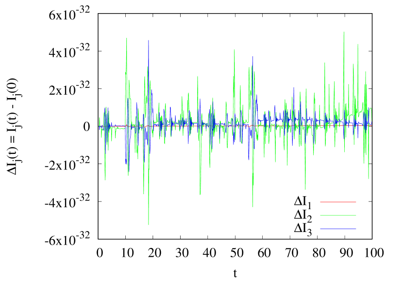
Figure 1: Numerical errors $\Delta I_{1}=h|_{t=0}-h_{0}$, $\Delta I_{2}=-\textstyle\frac{1}{2}\bm{q}\bm{p}|_{t=0}+\textstyle\frac{1}{2}\bm{q}_{0}\bm{p}_{0}$, and $\Delta I_{3}=\textstyle\frac{1}{4}\bm{q}^{2}|_{t=0}-\textstyle\frac{1}{4}\bm{q}_{0}^{2}$ of the invariants $I_{1}=h|_{t=0}$, $I_{2}=-\textstyle\frac{1}{2}\bm{q}\bm{p}|_{t=0}$, and $I_{3}=\textstyle\frac{1}{4}\bm{q}^{2}|_{t=0}$, calculated with quadruple precision.

With the potential of this system being of third order, the singularity of $g_{2}(t)$ at $(x(t),y(t))=(0,0)$ is removable. Setting $C=1$ and fixing the system’s dimensionless energy to the limiting value of $h=1/6$ for a bounded motion, we obtain for the initial condition $(x_{0},p_{x,0},y_{0},p_{y,0})=(0,0.5367,-0.2,0)$ the Poincaré surface-of-section displayed on the left-hand-side of Fig. 2. The points in this figure display the $(y,p_{y})$-coordinates of the particle in the course of its time evolution whenever its $x$-coordinate satisfies the condition $x=0$. The picture shows that almost the entire available phase-space area is covered in the course of the trajectory’s time evolution—which indicates that this particular trajectory is irregular. As each of these points can be considered by itself as an initial condition, we conclude that the vast majority of initial conditions that are associated with the energy $h=1/6$ give rise to irregular orbits.

Figure 2: Left: $y,p_{y}$-Poincaré surface-of-section representation of an irregular trajectory in the Hénon-Heiles oscillator (27) with the limiting energy $h=1/6$ for the initial condition $(x_{0},p_{x,0},y_{0},p_{y,0})=(0,0.5367,-0.2,0)$ and $C=1$. Right: Lyapunov function $\lambda_{1}(t)$ from Eq. (26) for this trajectory.

Figure 3: Left: real-space projection of a regular trajectory of the Hénon-Heiles oscillator (27) with the limiting energy $h=1/6$ as obtained for the initial condition $(x_{0},p_{x,0},y_{0},p_{y,0})=(0,0.3765,0.55,0)$ and $C=1$. Right: Lyapunov function $\lambda_{1}(t)$ from Eq. (26) for this trajectory.

In contrast, the blank areas within the dotted region correspond to the disjunct volume of phase space where the motion is regular. A regular trajectory is displayed in the picture on the left of Fig. 3 in the form of a real space projection of the phase-space motion. It is obtained by choosing the particle’s initial conditions to lie within the blank islands of the Poincaré surface-of-section of Fig. 2. We observe in the picture on the left of Fig. 3 that the particle crosses the vertical line $x=0$ exactly four times in the course of one oscillation period at different slopes $p_{y}$. These four locations correspond to the four blank islands occurring in the Poincaré section of Fig. 2. The occurrence of islands of finite area in the phase-space plane of Fig. 2 indicates that a regular motion is not only given for the strictly closed “clover-leaf” motion but also for an oscillation of some finite amplitude around this closed trajectory. A Poincaré surface-of-section of such a trajectory, together with its Lyapunov function $\lambda_{1}(t)$, is displayed in Fig. 4.

Figure 4: Left: $y,p_{y}$-Poincaré surface-of-section representation of a regular trajectory near the boundary of the regular region with the limiting energy $h=1/6$ as obtained for the initial condition $(x_{0},p_{x,0},y_{0},p_{y,0})=(0,0.3420,0.60,0.02)$ and $C=1$.
Right: Lyapunov function $\lambda_{1}(t)$ from Eq. (26) for this trajectory.

Figure 5: Right: enlarged view of the Lyapunov function $\lambda_{1}(t)$ from Fig. 2 for the time interval $75\times 10^{3}\leq t\leq 80.5\times 10^{3}$. Left: subset of the $y,p_{y}$-Poincaré-section points of Fig. 2 that emerges during that particular time interval.

Figure 6: Right: enlarged view of the Lyapunov function $\lambda_{1}(t)$ from Fig. 2 for the time interval $55\times 10^{3}\leq t\leq 60.5\times 10^{3}$. Left: subset of the $y,p_{y}$-Poincaré-section points of Fig. 2 that emerges during that particular time interval.

According to Theorem 2, the existence of a sharp asymptotic value of $\lambda_{1}(t)$ indicates the regularity of the respective trajectory $(x(t),y(t))$, i.e.,

$$\lambda_{1}^{i}=\lambda_{1}^{s}=\lim_{t\to\infty}\lambda_{1}(t)\Longleftrightarrow\text{regular\;trajectory}.$$ (28)

The solutions $\lambda_{1}(t)$ of Eq. (26) for the regular particle motions $(x(t),y(t))$ are displayed in the pictures on the right of Figs. 3 and 4. For these particular cases, the solution functions $\lambda_{1}(t)$ approach zero, hence converge to limit values. This is the expected result for regular trajectories.

In contrast, we observe in the picture on the right of Fig. 2 that the function $\lambda_{1}(t)$ associated with the irregular particle motion does not converge to a limit value. From Theorem 2, we conclude that the underlying trajectory is irregular—which is in agreement with the impression obtained from the Poincaré section of Fig. 2.

Furthermore, we can show for a chaotic trajectory that the detailed shape of the Lyapunov functions in the course of the system’s time evolution allows us to identify time intervals where the motion is temporarily quasiregular. In Fig. 5, we display an excerpt of Fig. 2 for the time interval $75\times 10^{3}\leq t\leq 80.5\times 10^{3}$. The right-hand-side plot of Fig. 5 shows that—apart from local fluctuations—the $\lambda_{1}$ curve decreases monotonicly in that time interval. This behavior of $\lambda_{1}$ resembles the regular cases displayed in Figs. 3 and 4. The section points occurring during this particular time interval are shown in the left-hand side of Fig. 5. We observe that these points are not spread over the possible phase-space region as one would expect for a chaotic motion with regard to the Poincaré section of Fig. 2. Instead, all section points are located in the vicinity of the four blank islands of Fig. 2. This arrangement of section points corresponds to a “clover-leaf”-like oscillation that is displayed in the left-hand-side picture of Fig. 3. We thus find that the chaotic trajectory is temporarily “trapped” into a quasiregular behavior.

A converse case is displayed in Fig. 6. The right-hand-side plot shows another enlarged portion of the graph of $\lambda_{1}(t)$ from Fig. 2, namely the time interval $55\times 10^{3}\leq t\leq 60.5\times 10^{3}$. In contrast to the behavior emerging in the case of Fig. 5, $\lambda_{1}$ keeps on fluctuating rapidly in that particular time interval and does not converge at times. The corresponding Poincaré-section points are shown on the left-hand side of Fig. 6. We observe that the section points are now spread over the entire available phase space. Thus, in this time interval, the system exhibits a purely chaotic behavior. Summarizing, we conclude that the detailed shape of the graph of $\lambda_{1}(t)$ provides us with information on the “instantaneous chaoticity” of the underlying trajectory.

IV.2 Nonlinear two-dimensional oscillator

We now investigate the chaos-order transitions of a model oscillator consisting of a two-dimensional harmonic oscillator that is disturbed by a fourth-order potential term depending on a coupling coefficient $C$. The characteristics of the trajectory as a function of the coupling coefficient $C$ in this two-dimensional Hamiltonian system was studied by Deng and Hioedeng . Its Hamiltonian is given in normalized form by

$$H(\bm{q},\bm{p})=\textstyle\frac{1}{2}(p_{x}^{2}+p_{y}^{2}+x^{2}+y^{2})+\mu(x^{4}+2Cx^{2}y^{2}+y^{4}).$$ (29)

The equations of motion following from Eq. (29) are

$$\ddot{x}+x+4\mu\left(x^{3}+Cxy^{2}\right)=0,\quad\ddot{y}+y+4\mu\left(y^{3}+Cx^{2}y\right)=0.$$ (30)

As the system (29) is autonomous, the coefficient $g_{1}(t)$ vanishes identically. For the Lyapunov stability analysis of the energy-second-moment map (11), we may therefore again restrict ourselves to solving the second-order system (26) and analyzing the single Lyapunov function $\lambda_{1}(t)$. For the particular potential of Eq. (29), the coefficient $g_{2}(t)$ is given by

$$g_{2}(t)=4+12\mu\,\frac{x^{4}(t)+2Cx^{2}(t)\,y^{2}(t)+y^{4}(t)}{x^{2}(t)+y^{2}(t)}.$$ (31)

Again, the point $(x(t),y(t))=(0,0)$ is a removable singularity of $g_{2}(t)$. In our numerical calculations, we used a fixed scaling parameter $\mu=1$. We compared the time evolution of the Lyapunov functions $\lambda_{1}(t)$ for different values of the coupling constant $C$. Following Deng and Hioe deng , we defined for the trajectory’s initial condition $x_{0}=5$, $y_{0}=10$, $p_{x,0}=p_{y,0}=0$ in all calculations.

Figure 7: Poincaré surfaces-of-section (left) and Lyapunov functions $\lambda_{1}(t)$ from Eq. (26) for different values of the coupling constant $C$ of the nonlinear 2D oscillator (29).

Figure 6: (Cont.) Poincaré surfaces-of-section (left) and Lyapunov functions $\lambda_{1}(t)$ from Eq. (26) for different values of the coupling constant $C$ of the nonlinear 2D oscillator (29).

For the coupling constants $C=-0.20$, $C=-0.17$, $C=-0.15$, as shown in Fig. 6, the Lyapunov functions (26) clearly approach limit values in the sense of Eq. (28), which indicates a regular motion each. The corresponding Poincaré surfaces-of-section show that the respective trajectories cross the plane $y=0$ only in the neighborhood of previous crossing points in the $(x,p_{x})$-phase-space plane. This depicts a quasiperiodic motion, which furnishes—on the long term—one or more closed curves in the Poincaré map.

In contrast, for coupling constants of $C=-0.21$, $C=-0.19$, $C=-0.18$, $C=-0.16$, limit values of the respective Lyapunov functions $\lambda_{1}(t)$ obviously do not exist. In complete agreement with this, the Poincaré surface-of-sections depicting the crossing points of the plane $y=0$ within the $(x,p_{x})$-phase-space plane show randomly scattered points. This reflects the fact that the motions are no longer quasiperiodic, hence that the respective trajectories are irregular.

IV.3 Circular restricted three-body system

As a third example, we apply our regularity analysis to the circular restricted three-body problemszebe of celestial mechanics. This system describes the motion of a body of negligible mass that is attracted by two heavy primary bodies. The primaries are assumed to follow circular orbits around their common center of mass and, secondly, not to be influenced by the presence of the third body. Working with normalized variables in the sideral (fixed) coordinate system, the equation of motion of the third body contains only one parameter $\mu$ and is explicitly time dependentszebe ; vela . The Hamiltonian of the third body is given by

$$H=\textstyle\frac{1}{2}\left(p_{x}^{2}+p_{y}^{2}+p_{z}^{2}\right)+V(x,y,z,t),$$ (32)

with the time-dependent potential

$$V(x,y,z,t)=-\frac{\mu}{\rho_{1}}-\frac{1-\mu}{\rho_{2}},$$ (33)

$$\qquad\rho_{1}^{2} \!=\!\! {\left[x-(1-\mu)\cos{t}\right]}^{2}+{\left[y-(1-\mu)\sin{t}\right]}^{2}+z^{2},$$

$$\qquad\rho_{2}^{2} \!=\!\! {\left(x+\mu\cos{t}\right)}^{2}+{\left(y+\mu\sin{t}\right)}^{2}+z^{2}.$$

The system parameter $\mu$ is determined by the ratio of the mass of one primary body to the system’s total mass. In the following, we will investigate the orbits of a light third body (e.g., a comet) in the Sun-Jupiter system with the mass parameter

$$\mu=\frac{m_{\text{J}}}{m_{\text{J}}+m_{\text{S}}}\approx 0.0009537,$$

where $m_{\text{J}}$ and $m_{\text{S}}$ are the masses of Jupiter and Sun, respectively. The canonical equations of the third body follow as

$$\dot{x} = p_{x},\quad\dot{y}=p_{y},\quad\dot{z}=p_{z},$$

$$\dot{p}_{x} = -\mu\frac{x-(1-\mu)\cos{t}}{\rho_{1}^{3}}-(1-\mu)\frac{x+\mu\cos{t}}{\rho_{2}^{3}},$$

$$\dot{p}_{y} = -\mu\frac{y-(1-\mu)\sin{t}}{\rho_{1}^{3}}-(1-\mu)\frac{y+\mu\sin{t}}{\rho_{2}^{3}},$$ (34)

$$\dot{p}_{z} = -\mu\frac{z}{\rho_{1}^{3}}-(1-\mu)\frac{z}{\rho_{2}^{3}}.$$

Since the Hamiltonian from Eq. (32) is explicitly time dependent, we must solve the third-order equation (8) to work out the Lyapunov functions (19) in order to quantify the irregularity of the third body’s motion. For the potential (33), the related coefficients $g_{1}(t)$ and $g_{2}(t)$ evaluate to

$$g_{1}(t) = \frac{4\mu(1-\mu)}{x^{2}+y^{2}+z^{2}}(x\sin{t}-y\cos{t})\left(\rho_{1}^{-3}-\rho_{2}^{-3}\right),$$

$$g_{2}(t) = \frac{-2}{x^{2}+y^{2}+z^{2}}$$ (35)

$$\quad\times\bigg{(}\mu\frac{\rho_{1}^{2}-(1-\mu)(x\cos{t}+y\sin{t}-[1-\mu])}{\rho_{1}^{3}}$$

$$\quad\mbox{}+(1-\mu)\frac{\rho_{2}^{2}+\mu(x\cos{t}+y\sin{t}+\mu)}{\rho_{2}^{3}}\bigg{)}.$$

In order to prevent the occurrence of large intermediate values, the actual numerical calculation of $\lambda_{1}(t)=-\lambda_{2}(t)-\lambda_{3}(t)$ is performed on the basis of Eqs. (21), (22) in place of the equivalent Eq. (8).

Figure 7: Poincaré surfaces-of-section (left) and Lyapunov functions $\lambda_{1}(t)$ from Eq. (19) for different initial conditions $x(0)$ of the circular restricted three-body problem of Eq. (IV.3) at $E=-1.515$.

Figure 7 shows the Poincaré surface-of-section and the Lyapunov function $\lambda_{1}(t)$ of Eq. (19) for different initial conditions for $x(0)$. Note that the corresponding initial conditions are given in the synodic, i.e., rotating coordinate system by $y(0)=0$, $p_{x}(0)=v_{x}(0)-y(0)=0$, $p_{y}(0)=v_{y}(0)+x(0)$, where $v_{y}(0)$ can be obtained from the value of the energy in the synodic system, i.e., $E=-1.515$ in the example studied (cf. the analysis of Ref. vela ). As has been shown in this paper, the initial value $x(0)=-1.5$ corresponds to the so called $2:3$ resonance island, where regular motion of the comet Oterma occurs with an almost constant frequency. In the related Poincaré surface-of-section this quasicyclic motion manifests itself as a single spot of finite width. If the initial value $x(0)$ is chosen outside of this resonance region, e.g., $x(0)=-2.2$, we observe a nonconverging time evolution of the Lyapunov function $\lambda_{1}(t)$. This indicates an irregular motion, which is in accordance with the corresponding Poincaré surface in Fig. 7.

V Conclusions

The method of deducing the degree of irregularity of Hamiltonian systems from the energy-second-moment map—rather than from a conventional stability matrix—was successfully illustrated by means of three examples. The energy-second-moment map was shown to be represented by the solution matrix of a linear, homogeneous third-order equation that is solvable on the top of the complete set of canonical equations. In terms of the solutions of this third-order equation, the Lyapunov functions of the energy-second-moment map turned out to have simple analytical representations. The existence of analytical representations of the Lyapunov functions of the energy-second-moment map simplifies significantly the irregularity analysis of Hamiltonian systems. This is the main benefit of our approach and applies to all systems whose Hamiltonian can be converted into the generic form $H=\bm{p}^{2}/2+V(\bm{q},t)$.

The conventional stability matrix analysis is based on the relative motion of infinitesimally separated trajectories. In contrast, the energy-second-moment-map analysis deals with the dependence of a single trajectory on its initial state, which, in terms of the energy-second moment vector $\bm{s}$, is represented by a linear transformation. From this viewpoint, our approach corresponds to the visual analysis that is provided by a Poincaré surface-of-section. The latter provides the information on the system’s irregularity through the fractal dimension of the set of intersections of a single trajectory with the surface-of-section and likewise does not take into account the relative motion of neighboring trajectories.

Maple worksheet for the symbolic calculation of Eqs. (19) from Eq. (9)

> with(linalg):
> # define matrix Xi(t) [Eq. (9)]
> Xi:=matrix(3,3,[xi1(t),xi2(t),xi3(t),
    diff(xi1(t),t),diff(xi2(t),t),
    diff(xi3(t),t),diff(xi1(t),t$2),
    diff(xi2(t),t$2),diff(xi3(t),t$2)]);

$$\Xi:=\left(\begin{array}[]{ccc}\xi{1}(t)&\xi{2}(t)&\xi{3}(t)\\ \frac{d}{dt}\xi{1}(t)&\frac{d}{dt}\xi{2}(t)&\frac{d}{dt}\xi{3}(t)\\ \frac{d^{2}}{dt^{2}}\xi{1}(t)&\frac{d^{2}}{dt^{2}}\xi{2}(t)&\frac{d^{2}}{dt^{2}}\xi{3}(t)\end{array}\right)$$

> # QR decomposition of Xi(t) [Eq. (15)]
> R:=QRdecomp(Xi, Q=’q’):
> R:=simplify(R,{det(Xi)=1}):
> # evaluate inverse of R(t)
> Rinv:=inverse(R):
> # evaluate time derivative of R(t)
> Rdot:=matrix(3,3,[diff(R[1,1],t),
      diff(R[1,2],t),diff(R[1,3],t),
      diff(R[2,1],t),diff(R[2,2],t),
      diff(R[2,3],t),diff(R[3,1],t),
      diff(R[3,2],t),diff(R[3,3],t)]):
> # evaluate B(t) [Eq. (16)]
> B:=evalm(Rdot &* Rinv):
> # test trace of B(t)
> TrB:=simplify(B[1,1]+B[2,2]+B[3,3]);
                            TrB := 0
> # evaluate lambda_2(t), lambda_3(t),
> #          lambda_1(t) [Eq. (17)]
> lambda[2]:=int(B[1,1],t)/t;

$$\lambda_{2}:=\frac{1}{2t}\ln\left[\xi 1(t)^{2}+{\left(\frac{d}{dt}\xi 1(t)\right)}^{2}+{\left(\frac{d^{2}}{dt^{2}}\xi 1(t)\right)}^{2}\right]$$

> lambda[3]:=int(B[3,3],t)/t;
> lambda[1]:=-lambda[2]-lambda[3].

References

- (1) A. M. Lyapunov, Problème général de la stabilité du mouvement, Annals of Mathematics Studies No. 17 (Princeton University Press, Princeton NJ, 1949).
- (2) H.-D. Mayer, J. Chem. Phys. 84, 3147 (1985).
- (3) V. B. Ryabov, Phys. Rev. E 66, 016214 (2002).
- (4) J. Struckmeier, J. Phys. A 38, 1257 (2005).
- (5) L. Ya. Adrianova, Introduction to Linear Systems of Differential Equations (American Mathematical Society, Providence, 1995).
- (6) L. Dieci and E. van Vleck, SIAM (Soc. Ind. Appl. Math.) J. Numer. Anal. 6, 516 (2002).
- (7) M. B. Monagan, K. O. Geddes, K. M. Heal, G. Labahn, S. M. Vorkoetter, J. McCarron, and P. DeMarco, Maple 10 Introductory Programming Guide, (Maplesoft, a division of Waterloo Maple Inc., Waterloo, Ontario, 2005).
- (8) S. Habib and R. D. Ryne, Phys. Rev. Lett. 74, 70 (1995); G. Rangarajan, S. Habib, and R. D. Ryne, ibid. 80, 3747 (1998).
- (9) M. Hénon, Numerical Exploration of Hamiltonian Systems, 1981 Les Houches École d’Été de Physique Théoretique, edited by G. Iooss, R. H. G. Helleman, and R. Stora (North-Holland, New York, 1983).
- (10) A. J. Lichtenberg and M. A. Lieberman, Regular and Chaotic Motion (Springer, New York, 1992).
- (11) H. Goldstein, C. Poole, and J. Safko, Classical Mechanics, 3rd ed. (Pearson, Addison-Wesley, Upper Saddle River, NJ, 2002).
- (12) R. Abraham and J. E. Marsden, Foundations of Mechanics, 2nd ed. (Westview Press, Boulder, CO, 1978).
- (13) Z. Deng and F. T. Hioe, Phys. Rev. Lett. 55, 1539 (1985).
- (14) V. Szebehely, Theory of Orbits (Academic Press, New York, 1967).
- (15) L. V. Vela-Arevalo and J. E. Marsden, Class. Quantum Grav. 21, 351 (2004).