Simulation-based Inference for Model Parameterization on Analog Neuromorphic Hardware

Abstract

The system implements physical models of neurons as well as synapses and aims for an energy-efficient and fast emulation of biological neurons. When replicating neuroscientific experiments on , a major challenge is finding suitable model parameters. This study investigates the suitability of the algorithm for parameterizing a multi-compartmental neuron model emulated on the analog neuromorphic system. The algorithm belongs to the class of methods and estimates the posterior distribution of the model parameters; access to the posterior allows quantifying the confidence in parameter estimations and unveiling correlation between model parameters.

For our multi-compartmental model, we show that the approximated posterior agrees with experimental observations and that the identified correlation between parameters fits theoretical expectations. Furthermore, as already shown for software simulations, the algorithm can deal with high-dimensional observations and parameter spaces when the data is generated by emulations on .

These results suggest that the algorithm is a promising approach for automating the parameterization and the analyzation of complex models, especially when dealing with characteristic properties of analog neuromorphic substrates, such as trial-to-trial variations or limited parameter ranges.

Keywords: analog $|$ neuromorphic $|$ simulation-based inference $|$ multi-compartment

1 Introduction

Mechanistic models, which try to explain the causality between inputs and outputs, are integral to scientific research. On the one hand they can increase the understanding of the mechanisms which cause the phenomena and on the other make predictions about new outcomes which can then be tested experimentally [baker2018mechanistic]. After a mechanistic model has been formulated, one of the remaining challenges is to find suitable model parameters which lead to a close agreement between model behavior and experimental observations.

Several approaches such as the hand-tuning of parameters, grid searches, random/stochastic searches, evolutionary algorithms, simulated annealing and particle swarm algorithms have been used in neuroscience to find appropriate model parameters [vanier1999comparative, vangeit2008automated]. Drawbacks of these methods are that they rely on a score which represents how close the results of a simulated model are to the target observation and that they in general only yield the best performing set of parameters. Furthermore, these algorithms are often computationally expensive since they require many simulations to find suitable parameters [goncalves2020training].

The class of algorithms makes statistical inference methods available for models where the likelihood is not tractable and provides an approximation of the posterior distribution of the model parameters. Advantages of deriving an approximation of the posterior include the possibility to find correlations between model parameters and to evaluate the confidence in the estimated parameters. Early approaches rely on defining a score and are computationally inefficient since they disregard many simulation which have a low score [sisson2018handbook].

Recent advances in machine learning lead to a new class of algorithms which promise to be computationally more efficient and do not depend on a score function [papamakarios2016fast, lueckmann2017flexible, greenberg2019automatic, cranmer2020frontier, deistler2022truncated]. In this paper we will focus on the algorithm which was already applied to infer parameters for different neuroscientific models [lueckmann2017flexible, goncalves2020training]. More specifically, we want to investigate if this algorithm is suitable to parameterize neuron models which are emulated on the analog neuromorphic hardware system [pehle2022brainscales2_nopreprint_nourl].

Neuromorphic computation draws inspiration from the brain to find time and energy efficient computing architectures as well as algorithms [indiveri2011neuromorphic]. The system emulates the behavior of neurons and synapses on analog circuits in continuous time [billaudelle2022accurate] and does not solve the model equations mathematically like digital neuromorphic hardware [furber2012overview, davies2018loihi, mayr2019spinnaker].

In previous experiments on the system, hardware parameters were set by calibration routines, grid searches, gradient-based optimization or by hand-tuning [billaudelle2022accurate, cramer2022surrogate, pehle2023event, aamir2018dls3neuron, wunderlich2019advantages, kaiser2022emulating]. The hand-tuning of parameters can be tedious and relies on the domain-specific knowledge of the experimenter such that automated parameter-search methods are inevitable for complex problems [vanier1999comparative]. Similarly, a calibration routine can only be formulated if the relationship between parameters and observations is known. Depending on the dimensionality of the parameter space, grid searches and random searches can be computationally too expensive. The algorithm promises to find approximations of the posterior even if the parameter space is high-dimensional and the relationship between the parameters and the observation is unknown [lueckmann2017flexible, greenberg2019automatic, goncalves2020training].

Furthermore, the algorithm is designed for probabilistic models. This makes it a suitable choice for models which deal with intrinsic probabilistic behavior such as analog neuromorphic hardware which is subject to temporal noise.

In the present study we emulated a passive multi-compartmental neuron model on and investigated whether the algorithm can find suitable model parameters to reproduce previously recorded target observations. For a two-dimensional parameter space, we show that the approximated posterior derived with the algorithm agreeed with a grid search over the whole parameter space and that the correlations between model parameters are in agreement with theoretical predictions.

Finally, we extended the problem to a higher-dimensional (7) parameter space and examined the approximated posteriors with . The correlations between parameters of this high-dimensional model did agree with the model equations.

All in all, our results indicate that the algorithm is able to deal with the intrinsic trial-to-trial variations of analog neuromorphic hardware and is able to approximate posterior distributions which are in agreement with the given target observations.

2 Methods

This section starts by introducing the neuromorphic system. We chose the attenuation of in a passive chain of compartments to test if the algorithm is capable to parameterize experiments on . Therefore, we introduce the attenuation experiment before we describe the algorithm. We conclude this section by introducing methods which we used to validate our posterior approximations.

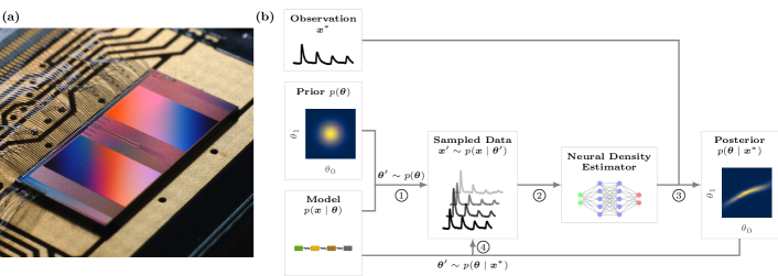
Figure 1: The bss2 system and the snpe algorithm. (a) Photograph of the bss2 neuromorphic chip bonded to a carrier board. (b) Visualization of the snpe algorithm [papamakarios2016fast, lueckmann2017flexible, greenberg2019automatic]. This algorithm can be used to find an approximation for the posterior distribution $p(\bm{\theta}\mid\bm{x}^{*})$ of parameters $\bm{\theta}$ which recreate a target observation $\bm{x}^{*}$. The target observation $\bm{x}^{*}$, a prior belief about the parameter distribution $p(\bm{\theta})$ and a model which gives implicit access to the likelihood $p(\bm{x}\mid\bm{\theta})$ are given as inputs to the algorithm. In step 1, we sample parameters $\bm{\theta}^{\prime}$ from the prior distribution and the model is evaluated with these parameters to obtain observations $\bm{x}^{\prime}$. This implicitly allows us to sample form the likelihood $p(\bm{x}\mid\bm{\theta}^{\prime})$. In the following step 2, the set of parameters and the corresponding observations are used to train a nde. The nde serves as a surrogate for the posterior distribution $p(\bm{\theta}\mid\bm{x})$. Frequently, we are interested in a single observation $\bm{x}^{*}$ and we can restrict the nde to this observation, step 3. We can now use samples drawn from the posterior $\bm{\theta}^{\prime}\sim p(\bm{\theta}\mid\bm{x}^{*})$ to generate new samples and retrain the nde, repeating step 2 and 3. Steps 2 to 4 can be repeated several times to improve the estimate of the posterior. The figure is based on [goncalves2020training, Figure 1].

2.1 bss2

is a mixed-signal analog neuromorphic system; neuron and synapse dynamics are emulated by analog circuits while spike events and configuration data rely on digital communication, Figure 1(a). More specifically, the dynamics of the analog neuron circuits are designed to resemble the dynamics of the neuron model [brette2005adaptive, billaudelle2022accurate]. Voltages and currents on these analog circuits directly represent the state of the emulated neuron.

2.1.1 Neuron Dynamics

The neuron model extends the neuron model by introducing an exponential and an adaptation current [brette2005adaptive]. The high configurability, see below, of the system allows disabling these currents to model neurons. Furthermore, several neuron circuits can be connected to form multi-compartmental neuron models [kaiser2022emulating].

In this publication, we will consider multi-compartmental neuron models for which the membrane potentials in the different compartments $V_{\text{m}}$ adhere to the dynamics of the neuron model,

$$C_{\text{m}}\derivative{V_{\text{m}}(t)}{t}=g_{\text{leak}}\cdot\left(V_{\text{leak}}-V_{\text{m}}(t)\right)+I_{\text{syn}}(t)+I_{\text{axial}}(t),$$ (1)

where $C_{\text{m}}$ is the membrane capacitance, $g_{\text{leak}}$ the leak conductance and $V_{\text{leak}}$ the leak potential.

The two currents in Equation 1 arise due to synaptic input, $I_{\text{syn}}$, and connections to neighboring compartments, $I_{\text{axial}}$. The synaptic current $I_{\text{syn}}$ models current-based synapses with an exponential kernel. The current $I_{\text{axial},i}(t)$ on compartment $i$ due to neighboring compartments is given by

$$I_{\text{axial},i}(t)=\sum_{j}g_{\text{axial}}^{i\leftrightarrow j}\cdot\left(V_{\text{m,j}}(t)-V_{\text{m,i}}(t)\right),$$ (2)

where the sum runs over all neighboring compartments $\{j\}$, $g_{\text{axial}}^{i\leftrightarrow j}$ represents the conductance between these compartments and $V_{j}$ is the membrane potential of the neighboring compartment.

Once the membrane potential $V_{\text{m}}$ crosses a threshold potential $V_{\text{thres}}$ a spike is generated and the membrane potential is reset to the reset potential $V_{\text{reset}}$. After the refractory time $\tau_{\text{ref}}$ the reset is released and the membrane potential $V_{\text{m}}$ continues to adhere to the dynamics of Equation 1.

2.1.2 Configurability

The behavior of the neuron circuits on can be controlled by several digital and analog parameters.

Digital parameters, for example, control if the adaptation or exponential currents are connected to the membrane [billaudelle2022accurate] and how different neuron circuits are connected to each other to form multi-compartmental neuron models [kaiser2022emulating].

Analog reference voltages and currents control quantities such as the leak conductance $g_{\text{leak}}$, leak potential $V_{\text{leak}}$ or the axial conductance $g_{\text{axial}}$ between neuron circuits. These analog references are provided by an analog on-chip memory array which converts digital $10\text{\,}\mathrm{bit}$ values to currents and voltages [hock13analogmemory]. Since the last value is reserved, reference currents and voltages can be adjusted digitally from $01022$. This large configuration range allows tuning the neuron circuits to a variety of different operating regimes and to compensate manufacturing-induced mismatch between different neuron circuits [billaudelle2022accurate].

In the current publication, we use the latest revision of the system [pehle2022brainscales2_nopreprint_nourl, billaudelle2022accurate]. The PyNN domain-specific language [davison2009pynn] was used to formulate the experiments and the OS to define as well as to control the experiments [mueller2020bss2ll_nourl].

2.2 Experiment Description - A Linear Chain of Compartments

In order to test the capabilities of the algorithm, we considered a multi-compartmental model which consisted of a chain of passive compartments, see Figure 2(a). Such multi-compartmental models have been used to model dendrites and axons [rall1962electrophysiology, fatt1951analysis]. Each compartment $i$ was connected to a leak potential $V_{\text{leak}}$ via a leak conductance $g_{\text{leak}}^{i}$ and to the neighboring compartment via an axial conductance $g_{\text{axial}}^{i\leftrightarrow i+1}$, compare Equation 2. These conductances served as our parameters $\bm{\theta}$, all other parameters were fixed.

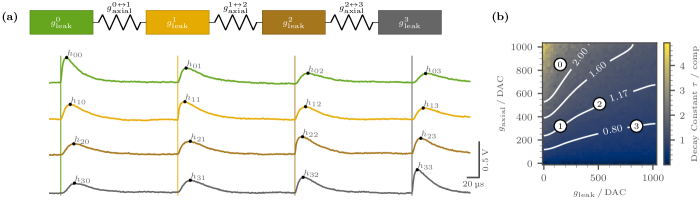
Figure 2: Model of a passive compartment chain and grid search results. (a) The parameters of the model are given by the leak conductance in each compartment $g_{\text{leak}}^{i}$ and the axial conductance between compartments $g_{\text{axial}}^{i\leftrightarrow i+1}$. In our experiment we observe the propagation of psp. Here we show membrane traces of neurons which were emulated on the bss2 system. We inject a synaptic input (vertical lines) in one compartment after another and record the membrane potential in each compartment (different rows). From these traces we extract the heights of the $h_{ij}$. We use the matrix of all heights $\bm{H}$, the heights resulting from an input to the first compartment $\bm{F}=[h_{00},h_{10},h_{20},h_{30}]$ or the decay constant $\tau$ from an exponential fit to $\bm{F}$ as observables. The scale bar in the lower right corner indicates the voltage and time in the hardware domain. (b) Grid search on bss2 of the decay constant $\tau$; the decay constant is given in units of “compartments” and calculated by fitting an exponential to the which result from an input to the first compartment, compare panel (a). We divided the parameter space in an evenly spaced grid with $40$ values in each dimension, recorded the resulting psp heights in each compartment and extracted the decay constant $\tau$; LABEL:fig:exponential shows the exponential fits for some exemplary measurements. The decay constant $\tau$ decreases as the leak conductance $g_{\text{leak}}$ is increased or the axial conductance $g_{\text{axial}}$ is reduced. The white contour lines mark regions with equal decay constant and show a correlation between leak and axial conductance. Traces recorded at the numbered points are displayed in Figure 3.

We injected synaptic inputs in the different compartments and observed how the propagate along the chain. More specifically, we looked at the heights of ; in the following we will use the notation $h_{ij}$ to describe the height which was observed in compartment $i$ after an input to compartment $j$, Figure 2(a). Since we were only interested in the passive propagation, we disabled the spiking threshold, this is equivalent to $V_{\text{thres}}\to\infty$.

Due to the low-pass properties of the passive chain, the response in the first compartment broadened and its height decreased as the synaptic input was injected further away from the first compartment, compare first row in Figure 2(a). A similar behavior was visible when we looked at the voltage traces in the second compartment: the broadened and flattened for inputs further away from the recording site. Since we considered a finite chain, we saw that an input at the end of the chain affected the membrane potential more strongly, for example $h_{10}>h_{12}$.

The height of the depended on the leak and axial conductance [fatt1951analysis]. A higher leak or axial conductance resulted in lower heights at the injection site as less charge can be accumulated on the compartment. Therefore, the heights $\bm{H}$ or quantities derived form them were suitable observations $\bm{x}$ that could be used to infer parameters $\bm{\theta}$. Besides the full matrix of heights, we used the heights which resulted from an input to the first compartment $\bm{F}=[h_{00},h_{10},h_{20},h_{30}]$ and the decay constant $\tau$ from an exponential fit to $\bm{F}$ as observables.

2.3 Sequential Neural Posterior Estimation Algorithm

The algorithm [papamakarios2016fast, lueckmann2017flexible, greenberg2019automatic] belongs to the class of algorithms and allows finding an approximation of the posterior distribution $p\left(\bm{\theta}\mid\bm{x}^{*}\right)$ in cases where the likelihood $p\left(\bm{x}\mid\theta\right)$ is intractable. Here $\bm{\theta}$ are the parameters of a mechanistic model for which we try to find parameters which reproduce a target observation $\bm{x}^{*}$. The main idea is to evaluate the model for different parameters $\{\bm{\theta}_{i}\}$, extract the observations $\{\bm{x}_{i}\}$ and fit a flexible probability distribution as a posterior to this set of parameters and observations. As the name suggests the parameters of these probability distributions are determined by neural networks.

The algorithm takes a target observation $\bm{x}^{*}$, prior $p(\bm{\theta})$ and a model for which suitable parameters should be found as an input, Figure 1(b). The prior is used to draw random parameters $\bm{\theta}^{\prime}\sim p(\bm{\theta})$. By executing the model with the given parameters $\bm{\theta}^{\prime}$ we implicitly sample from the likelihood $\bm{x}^{\prime}\sim p(\bm{x}\mid\bm{\theta}^{\prime})$. In our case the evaluation of the model is the emulation on the system.

In the second step, a is trained to approximate the posterior distribution $p(\bm{\theta}\mid\bm{x})$. The is a flexible set of probability distributions which are parameterized by a neural network. Typical choices are mixture-density networks [bishop1994mixture, papamakarios2016fast, lueckmann2017flexible, greenberg2019automatic] or [papamakarios2017masked, papamakarios2019sequential, goncalves2020training, papamakarios2021normalizing]. The is commonly trained by minimizing the negative log-likelihood of the previously drawn samples. Therefore, unlike traditional algorithms the algorithm does not depend on a user-defined score function. After successful training, the approximates the posterior distribution of the parameters for any observation $\bm{x}$.

If we are only interested in a single target observation $\bm{x}^{*}$, we can use the estimated posterior distribution in the following rounds as a proposal prior [papamakarios2016fast, lueckmann2017flexible, greenberg2019automatic]. While this sequential approach can increase sample efficiency, the obtained approximation of the posterior is no longer amortized, i.e. it can only be used to infer parameters for the target observation $\bm{x}^{*}$ and not any arbitrary observation $\bm{x}$.

In our experiments we applied the algorithm presented in [greenberg2019automatic] which is implemented in the Python package sbi [tejero2020sbi]. The structure of the as well as other hyperparameters of the algorithm can be found in LABEL:sec:meth:snpe.

2.4 Validation

In order to validate the approximated posteriors we used and calculated the expected coverage for each posterior [hermans2022crisis].

2.4.1 Predictive Posterior Check

We performed to check if an approximated posterior $p\left(\bm{\theta}\mid\bm{x}^{*}\right)$ yielded parameters $\bm{\theta}$ which are in agreement with the original observation $\bm{x}^{*}$. As discussed in [lueckmann2021benchmarking], do not measure the similarity of the approximated and true posterior and should just be used as a check rather than a metric. Nevertheless, we found that were sensitive enough to highlight posterior approximations which did not agree with our expectation of the posterior based on grid search results. In the appendix, we illustrate examples of mismatching posteriors, LABEL:fig:simulations, and show how we used to adjust the hyperparameters of the , LABEL:fig:transforms.

For all we drew $1000$ random parameters $\{\bm{\theta}_{i}\}$ from the approximated posterior $p\left(\bm{\theta}\mid\bm{x}^{*}\right)$, emulated the chain model with these parameters on and recorded the observables $\{\bm{x}_{i}\}$. We used the mean Euclidean distance between these observations and the target observation $\bm{x}^{*}$ as an indicator for an successful approximation.

2.4.2 Expected Coverage

Recent publications indicate that the posteriors approximated with the algorithm tend to yield overconfident posterior approximations, i.e. the posterior distribution is to narrow [hermans2022crisis, deistler2022truncated]. To test the confidence of our posteriors we calculated the expected coverage as suggested in [hermans2022crisis].

We calculated the expected coverage as follows. First we drew $1000$ random samples from the prior distribution, $\{\bm{\theta}_{i}^{*}\}\sim p(\bm{\theta})$. We then performed the experiment with these parameters on to obtain observations $\{\bm{x}_{i}^{*}\}$, yielding pairs $\{(\bm{\theta}^{*},\bm{x}^{*})_{i}\}\sim p(\bm{\theta},\bm{x})$. Finally, we calculated the coverage of each pair $(\bm{\theta}^{*},\bm{x}^{*})_{i}$ and averaged over them to get the expected coverage.

The coverage of a single pair was calculated as follows. We drew $10\,000$ samples for from the amortized posterior $\{\bm{\theta}^{\prime}_{j}\}\sim p(\bm{\theta}\mid\bm{x}_{i}^{*})$ for each pair (i.e. we performed the coverage tests with the first round approximations of the posterior and not the final approximations). Next, we used the posterior probability of the original parameter $p(\bm{\theta}^{*}\mid\bm{x}_{i}^{*})$ and of the drawn samples $\{p(\bm{\theta}^{\prime}_{j}\mid\bm{x}_{i}^{*})\}_{j}$ to estimate the coverage.

3 Results

To simplify the problem, we started by considering a two-dimensional parameter space. This was achieved by setting the leak and axial conductance globally. The low dimensionality of the parameter space allowed us to perform a grid search in a reasonable amount of time and to easily visualize the results. The grid search result can give an intuition about the behavior of the chain and was used as a comparison to the approximated posterior obtained with the algorithm.

We also executed the for a high-dimensional (7) parameter space and performed . For both, the two-dimensional and high-dimensional parameter space we looked at different kind of observations and how these influence the approximated posterior. Furthermore, we analyzed the correlation for each posterior and performed coverage tests.

3.1 Two-dimensional Parameter Space

We reduced the dimensions of the parameter space to two by setting the leak and axial conductance for all compartments and connections to the same digital value; $g_{\text{leak}}^{i}=g_{\text{leak}}\;\forall i\in\{0,1,2,3\}$ and $g_{\text{axial}}^{i\leftrightarrow i+1}=g_{\text{axial}}\;\forall i\in\{0,1,2\}$.

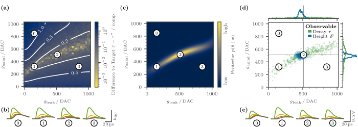
Figure 3: Propagation of psp in a passive chain of four compartments emulated on the bss2 system. Leak and axial conductance were set to the same value for all compartments and connections between compartments. (a) Grid search result illustrated as the difference of the measured decay constant $\tau$, compare Figure 2(b), to the target decay constant $\tau^{*}$: $\left|\tau-\tau^{*}\right|$. Traces recorded at the numbered points are displayed in panel (b) and (e). (b) Example traces recorded at different locations in the parameter space, compare panel (a). The colors of the traces indicate in which compartment the trace was recorded, compare Figure 2(a). The traces are scaled relative to the height in the first compartment $h_{00}$. Due to the faster emulation of the neural dynamics on , the time scales are in the microsecond rather than in the millisecond range. (c) Posterior obtained with the snpe algorithm. The posterior shows a high density in the parameter region where the target decay constant $\tau^{*}$ was recorded, 2. As expected from the grid search result in panel (a), a correlation between the leak and axial conductance is visible. Points where the decay constant is significantly lower/higher than the target observation show a low probability density, 0 and 3. (d) $500$ random samples drawn from the approximated posteriors for two different types of observations. The green points represent samples drawn from the posterior which is shown in panel (c). The samples show a correlation between both parameters. If the absolute heights of the psp which resulted from an input to the first compartment $\bm{F}=[h_{00},h_{10},h_{20},h_{30}]$ was chosen as observations (blue), the samples scatter around point 2 where the original target $\bm{F}^{*}$ was recorded. The histograms at the top and right of the scatter plot show histograms of the parameter distribution in one dimension. (e) Same traces as in panel (b) but shown on an absolute scale. While traces 1 and 2 share a similar decay constant $\tau$, compare panel (a) and (b), their absolute heights differs.

3.1.1 Grid Search

In order to obtain an overview of the model behavior, we performed a grid search over the two-dimensional parameter space. We created a grid of parameters by choosing equally spaced values of the leak and axial conductance which span the whole parameter range. The model was then emulated with these parameters on the system and the membrane traces in the different compartments were recorded. In order to easily visualize the results, we selected a one-dimensional observable. Exponential fits to the maximal height of propagating were used in other publications to classify the attenuation of in apical dendrites [berger2001high]. Similarly, we fitted an exponential to the heights which resulted from an input to the first compartment $\bm{F}=[h_{00},h_{10},h_{20},h_{30}]$ and analyzed the exponential decay constant $\tau$, Figure 2(b). The decay constant increased with increasing axial conductance $g_{\text{axial}}$ and decreasing leak conductance $g_{\text{leak}}$. Even though the exponential is just an approximation for the attenuation of transient inputs in multi-compartmental models, a correlation between leak and axial conductance is expected [fatt1951analysis, rall1962electrophysiology]. This behavior can also be understood with Equations 1 and 2: a lower leak conductance $g_{\text{leak}}$ leads to less charge leaking from the membrane and consequently a larger charge transfer to the neighboring compartments, which can be counterbalanced by a lower axial conductance $g_{\text{axial}}$.

The responses of the membrane potentials to a synaptic input in the first compartment are displayed in Figure 3(b). For a low leak and a large axial conductance, 0, the attenuation was the weakest and the was still clearly visible in the last compartment. Parameters on the same contour line showed, as expected, similar attenuation, 1 and 2, even though the exact shape of the differed. For a large leak and a low axial conductance, 3, the decayed quickly and almost vanished in the third compartment.

3.1.2 Simulation Based Inference

We used the algorithm to infer possible parameters $\bm{\theta}=[g_{\text{leak}},g_{\text{axial}}]$ which reproduce a target observation $\bm{x}^{*}=[\tau^{*}]$. Furthermore, we investigated how the posterior distribution changed when a more informative observation $\bm{x}^{*}=\bm{F}^{*}=[h_{00}^{*},h_{10}^{*},h_{20}^{*},h_{30}^{*}]$ was used, compare Figure 2(a).

In the case where a target observation $\bm{x}^{*}$ is given by an experiment, the true posterior and the optimal model parameters which replicate the observation are typically unknown. This makes it hard to assess the quality of the posterior approximated by the algorithm. Therefore, we explicitly chose target parameters $\bm{\theta}^{*}$, emulated our model with these parameters on and measured an “artificial” target observation $\bm{x}^{*}=\tau^{*}$. This allowed us to perform a closure test and check whether the algorithm was able to estimate a posterior which agreed with the initial observation.

We picked a target parameter $\bm{\theta}^{*}$ at the center of the parameter space and executed the model with this parameter $100$ times to account for trial-to-trial variations due to temporal noise. From the full matrix of heights $\bm{H}$ we extracted different target observations such as the decay constant $\tau$. The mean of the observed decay constants was our target observation $\bm{x}^{*}=[\overline{\tau}^{*}]=1.17\pm 0.04$; the decay constant is in units of “compartments”. In contrast, while running the algorithm we executed the model just once for each parameter and did not average over several trials.

We used a uniform distribution over all possible parameters as a prior distribution $p(\bm{\theta})$ and executed the