Squeezed bispectrum and one-loop corrections in transient constant-roll inflation

Abstract

In canonical single-field inflation, the production of primordial black holes (PBH) requires a transient violation of the slow-roll condition. The transient ultra slow-roll inflation is an example of such scenarios, and more generally, one can consider the transient constant-roll inflation. We investigate the squeezed bispectrum in the transient constant-roll inflation and find that Maldacena’s consistency relation holds for a sufficiently long-wavelength mode, whereas it is violated for modes around the peak scale for the non-attractor case. We also demonstrate how the one-loop corrections are modified compared to the case of the transient ultra slow-roll inflation, focusing on representative one-loop terms originating from a time derivative of the second slow-roll parameter in the cubic action. We find that the perturbativity requirement on those terms does not rule out the production of PBH from the transient constant-roll inflation. Therefore, it is a simple counterexample of the recently claimed no-go theorem of PBH production from single-field inflation.

1 Introduction

PBH [1, 2, 3, 4], hypothetical black holes formed in the early universe before any star-forming, are attracting attention more and more. They can explain a dominant component of dark matter [5], black-hole-merger events discovered by the LIGO–Virgo–KAGRA collaborations [6], microlensing events towards the Galactic bulge generated by planetary-mass objects [7], possible origins of supermassive black holes [8], early massive galaxies discovered by the James Webb Space Telescope [9, 10], etc. (see a recent review [11]).

One of the main formation scenarios of primordial black holes is the collapse of order-unity overdensities associated with large primordial perturbations generated, e.g., by cosmic inflation. In the canonical single-field inflation scenario, the enhancement of the primordial perturbation amplitude necessary for production of sizable amount of PBHs requires a transient violation of slow-roll [12]

$$\frac{\Delta\ln\epsilon}{\Delta N}\lesssim-0.4.$$ (1.1)

where $\epsilon=-\dot{H}/H^{2}$ is the first slow-roll parameter and $N=\int H\differential{t}$ is the e-folding number. It implies that a large value of the second slow-roll parameter $\eta=\dot{\epsilon}/(\epsilon H)$. A special case $\eta=-6$ is known as the ultra slow-roll limit [13, 14], and the transient ultra slow-roll inflation has been extensively studied recently as one of the representative models of the PBHs production [15, 16, 17, 12, 18, 19, 20, 21, 22, 23, 24, 25, 26, 27, 28, 29, 30, 31]. More generally, the constant $\eta$ phase is called constant-roll inflation. The constant-roll inflation [32, 33, 34, 35] allows an exact solution satisfying a condition of the constant rate of roll, $\ddot{\phi}/(H\dot{\phi})=\beta$ with constant $\beta$, for which $\eta\approx 2\beta$ holds. It is often used a scenario to generate a red-tilted spectrum compatible with cosmic microwave background (CMB) observations [33, 36, 37, 38], but using a different parameter range, it can also generate a blue-tilted spectrum in non-/attractor dynamics, which can be utilized to PBH production [39, 40, 41, 42].

In the context of PBH production, not only the amplitude of the power spectrum but also the non-Gaussian feature of the primordial perturbation is important as it affects the mean abundance (see, e.g., Refs. [43, 44, 45, 46, 47, 48, 49, 50, 51, 52, 53, 23, 54, 55, 56, 57, 58, 59]), the spatial distribution (clustering) (see, e.g., Refs. [60, 61, 62, 63, 64, 65, 66]), the corresponding induced gravitational wave (GW) (see, e.g., Refs. [67, 68, 69, 70, 71] and also Ref. [72] for a recent review), etc. Also, the one-loop corrections have been actively discussed recently in the context of whether the PBH production in the canonical single-filed inflation is ruled out from the perturbativity requirement [73, 74, 75, 76, 77, 78, 79, 80, 81]. While previous researches mainly focused on the PBH production in the transient ultra slow-roll inflation, as stressed above, it is not the unique option even within the canonical single-field inflation. The non-Gaussianity and one-loop corrections in other single-field scenarios remain unclear.

In this paper, we investigate the non-Gaussianity and one-loop corrections in the transient constant-roll model. After reviewing the transient constant-roll inflation in §2, we consider the squeezed bispectrum in §3, evaluated on both regimes after and during the constant roll phase. We clarify the cases where the Maldacena’s consistency relation [82] is satisfied or violated. In §4, focusing on representative terms, which originate from $\dot{\eta}$ term in the cubic action, we demonstrate how the one-loop corrections are modified compared to the case of the transient ultra slow-roll inflation. We find that the perturbativity requirement on those terms does not rule out the production of PBHs from the transient constant-roll inflation. §5 is devoted to conclusions. Throughout the paper, we work in the Planck units where $c=\hbar=M_{\mathrm{Pl}}=1$.

2 Transient constant-roll inflation

Let us review brief features of the constant-roll phase, assuming a toy transient model. In this model, the constant-roll phase is inserted in the slow-roll inflation and each phase is characterized by the second slow-roll parameter

$$\eta=\frac{\dot{\epsilon}}{\epsilon H}=\begin{cases}0,&\tau<\tau_{\mathrm{s}},\\ 2\beta,&\tau_{\mathrm{s}}\leq\tau<\tau_{\mathrm{e}},\\ 0,&\tau_{\mathrm{e}}\leq\tau,\end{cases}$$ (2.1)

where $\beta$ is a constant. To generate a blue-tilted spectrum for PBH production, we focus on the constant-roll model with a negative value of $\beta$. $\tau<0$ is the conformal time and $\tau_{\mathrm{s}(\mathrm{e})}$ represents the onset (end) of the constant-roll phase. $\beta=-3$ corresponds to the ultra slow-roll inflation. While $\beta<-3/2$ yields a non-attractor dynamics, $-3/2<\beta<0$ follows an attractor solution and the curvature perturbation gets frozen in the superhorizon limit [33, 83, 84, 85, 39]. We assume that the first slow-roll parameter $\epsilon$ is small enough and the Hubble parameter $H=\dot{a}/a$ ($a$ is the global scale factor) is almost constant during inflation. It is then solved as

$$\epsilon=-\frac{\dot{H}}{H^{2}}=\begin{cases}\epsilon_{\mathrm{SR}1},&\tau<\tau_{\mathrm{s}},\\ \epsilon_{\mathrm{SR}1}\pqty{\frac{\tau}{\tau_{\mathrm{s}}}}^{-2\beta},&\tau_{\mathrm{s}}\leq\tau<\tau_{\mathrm{e}},\\ \epsilon_{\mathrm{SR}2}=\epsilon_{\mathrm{SR}1}\pqty{\frac{\tau_{\mathrm{e}}}{\tau_{\mathrm{s}}}}^{-2\beta},&\tau_{\mathrm{e}}\leq\tau,\end{cases}$$ (2.2)

with the constant initial value $\epsilon_{\mathrm{SR}1}$. The slow-roll parameter $\epsilon$ decreases during the constant-roll phase and then the power spectrum of the curvature perturbation can be enhanced on the corresponding scales.

Let us see the linear dynamics of the curvature perturbation on the comoving slice, $\zeta(\tau,\mathbf{x})$. The corresponding quantum operator $\hat{\zeta}_{\mathrm{I}}(\tau,\mathbf{x})$ (i.e., $\hat{\zeta}$ in the interaction picture) is expanded by the annihilation-creation operator $\hat{a}_{\mathbf{k}}/\hat{a}_{\mathbf{k}}^{\dagger}$ as

$$\hat{\zeta}_{\mathrm{I},\mathbf{k}}(\tau)=\int\frac{\differential[3]\mathbf{k}}{(2\pi)^{3}}\pqty{\zeta_{k}(\tau)\hat{a}_{\mathbf{k}}+\zeta_{k}^{*}(\tau)\hat{a}_{-\mathbf{k}}^{\dagger}}\mathrm{e}^{i\mathbf{k}\cdot\mathbf{x}}.$$ (2.3)

The annihilation-creation operator satisfies the commutation relation

$$[\hat{a}_{\mathbf{k}},\hat{a}_{\mathbf{k}^{\prime}}^{\dagger}]=(2\pi)^{3}\delta^{(3)}(\mathbf{k}-\mathbf{k}^{\prime}),\quad[\hat{a}_{\mathbf{k}},\hat{a}_{\mathbf{k}^{\prime}}]=[\hat{a}^{\dagger}_{\mathbf{k}},\hat{a}^{\dagger}_{\mathbf{k}^{\prime}}]=0.$$ (2.4)

The mode function $\zeta_{k}(\tau)$ is governed by the Mukhanov–Sasaki equation

$$v_{k}^{\prime\prime}+\pqty{k^{2}-\frac{z^{\prime\prime}}{z}}v_{k}=0,$$ (2.5)

where the Mukhanov–Sasaki variable $v_{k}$ is related to $\zeta_{k}$ by $v_{k}=z\zeta_{k}$ with $z=a\sqrt{2\epsilon}$. The prime denotes the conformal time derivative. The effective mass term $z^{\prime\prime}/z$ is expressed in terms of slow-roll parameters as

$$\frac{z^{\prime\prime}}{z}=a^{2}H^{2}\left(2-\epsilon_{1}+\frac{3}{2}\epsilon_{2}+\frac{1}{4}\epsilon_{2}^{2}-\frac{1}{2}\epsilon_{1}\epsilon_{2}+\frac{1}{2}\epsilon_{2}\epsilon_{3}\right),$$ (2.6)

where $\epsilon_{1}=\epsilon$ and $\epsilon_{n+1}=H^{-1}\differential{\ln\epsilon_{n}}/\differential{t}$ (i.e., $\epsilon_{2}=\eta$). Both in the slow-roll (all slow-roll parameters are negligible) and constant-roll phases (slow-roll parameters except for $\eta$ are negligible), this can be rewritten as

$$\frac{z^{\prime\prime}}{z}=\frac{\nu^{2}-1/4}{\tau^{2}},$$ (2.7)

with

$$\nu=\begin{cases}\nu_{\mathrm{SR}}=3/2,&\text{slow-roll phase,}\\ \nu_{\mathrm{CR}}=\absolutevalue{3/2+\beta},&\text{constant-roll phase},\end{cases}$$ (2.8)

The solution of the Mukhanov–Sasaki equation is given by a superposition of the Hankel functions $\sqrt{-k\tau}H_{\nu}^{(1)}(-k\tau)$ and $\sqrt{-k\tau}H_{\nu}^{(2)}(-k\tau)$. Particularly in the slow-roll phase, the solution is simplified as

$$\zeta_{k}=\frac{iH}{2\sqrt{\epsilon k^{3}}}\bqty{\mathcal{A}_{k}\mathrm{e}^{-ik\tau}(1+ik\tau)-\mathcal{B}_{k}\mathrm{e}^{ik\tau}(1-ik\tau)},$$ (2.9)

with the constants of integration, $\mathcal{A}_{k}$ and $\mathcal{B}_{k}$. These coefficients are fixed by the Bunch–Davies initial condition

$$v_{k}\underset{\tau\to-\infty}{\to}\frac{\mathrm{e}^{-ik\tau}}{\sqrt{2k}},$$ (2.10)

and junction conditions at $\tau_{\mathrm{s}}$ and $\tau_{\mathrm{e}}$,

$$\zeta_{k}(\tau_{\mathrm{s}(\mathrm{e})}-0)=\zeta_{k}(\tau_{\mathrm{s}(\mathrm{e})}+0),\quad\zeta_{k}^{\prime}(\tau_{\mathrm{s}(\mathrm{e})}-0)=\zeta_{k}^{\prime}(\tau_{\mathrm{s}(\mathrm{e})}+0).$$ (2.11)

The (tree-level) power spectrum of the curvature perturbation is defined by

$$P_{\zeta}(k)=\absolutevalue{\zeta_{k}}^{2}.$$ (2.12)

The following dimensionless power is also useful.

$$\mathcal{P}_{\zeta}(k)=\frac{k^{3}}{2\pi^{2}}P_{\zeta}(k).$$ (2.13)

We show example spectra for various values of $\beta$ in Fig. 1. One can confirm that though it is small enough as $\mathcal{P}_{\zeta}\sim 2\times 10^{-9}$ to be consistent with the CMB observation on large scales $\gtrsim$1\text{\,}\mathrm{M}\mathrm{p}\mathrm{c}$$ [86], the power spectrum can be sufficiently large for PBH formation on a small scale even in the attractor models $-3/2<\beta<0$.

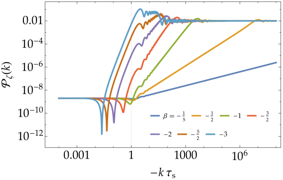
Figure 1: Example power spectra (2.13) in the late-time limit $\tau\to 0$ for $\beta=-1/5$ (blue), $-1/2$ (yellow), $-1$ (green), $-3/2$ (red), $-2$ (purple), $-5/2$ (brown), and $-3$ (turquoise). $\tau_{\mathrm{e}}/\tau_{\mathrm{s}}$ is determined by the condition $\epsilon_{\mathrm{SR}2}/\epsilon_{\mathrm{SR}1}=\pqty{\tau_{\mathrm{e}}/\tau_{\mathrm{s}}}^{-2\beta}=2\times 10^{-9}/10^{-2}$ so that $\mathcal{P}_{\zeta}\sim 2\times 10^{-9}$ on a large scale and $\mathcal{P}_{\zeta}\sim 10^{-2}$ on a small scale.

3 Squeezed bispectrum

The bispectrum $B_{\zeta}(k_{1},k_{2},k_{3})$, a three-point function in Fourier space, is defined by

$$\braket{\hat{\zeta}_{\mathbf{k}_{1}}\hat{\zeta}_{\mathbf{k}_{2}}\hat{\zeta}_{\mathbf{k}_{3}}}=(2\pi)^{3}\delta^{(3)}(\mathbf{k}_{1}+\mathbf{k}_{2}+\mathbf{k}_{3})B_{\zeta}(k_{1},k_{2},k_{3}),$$ (3.1)

where $\hat{\zeta}_{\mathbf{k}}$ is the Fourier mode of $\hat{\zeta}(\mathbf{x})$. In particular, its squeezed limit where one momentum is much smaller than the others is a useful indicator of the physics sourcing the curvature perturbation. It also affects the PBH formation. For example, the following local-type non-Gaussianity is known as a phenomenological model showing a non-zero squeezed bispectrum:

$$\hat{\zeta}(\mathbf{x})\approx\hat{g}(\mathbf{x})+\frac{3}{5}f_{\mathrm{NL}}\hat{g}^{2}(\mathbf{x}),$$ (3.2)

where $\hat{g}$ is a Gaussian random field and the coefficient $f_{\mathrm{NL}}$ is called the non-linearity parameter. At the leading order in the expansion in $\hat{g}$, the bispectrum and the non-linearity parameter are related by

$$B_{\zeta}(k_{1},k_{2},k_{3})\underset{k_{1}/k_{2}\ll 1}{\to}\frac{12}{5}f_{\mathrm{NL}}P_{\zeta}(k_{1})P_{\zeta}(k_{2}).$$ (3.3)

For a small-enough perturbation $\hat{g}\ll 1$, the non-Gaussian part (the second term) in Eq. (3.2) is subdominant as long as the non-linearity parameter is not so large, $f_{\mathrm{NL}}\lesssim\mathcal{O}(1)$. However, because PBHs are caused by the order-unity curvature perturbation, even the not-so-large non-Gaussianity $f_{\mathrm{NL}}\sim 1$ can significantly affect the PBH abundance (see, e.g., Refs. [43, 44, 45, 46, 47, 48, 49, 50, 51, 52, 67, 53, 23, 54, 55, 56, 57, 58, 59, 71]). The squeezed bispectrum also means the correlation between the long- and short-wavelength modes. Hence it can generate the large-scale modulation of the PBH spatial distribution known as the PBH bias or clustering (see, e.g., Refs. [60, 61, 62, 63, 64, 65, 66]). From this perspective, we investigate the details of the squeezed bispectrum in the transient constant-roll inflation model in this section. We often use the generalized non-linearity parameter defined by

$$f_{\mathrm{NL}}(k_{\mathrm{L}},k_{\mathrm{S}})=\frac{5}{12}\frac{B_{\zeta}(k_{\mathrm{L}},k_{\mathrm{S}},k_{\mathrm{S}})}{P_{\zeta}(k_{\mathrm{L}})P_{\zeta}(k_{\mathrm{S}})},$$ (3.4)

as a useful variable for the squeezed configuration $k_{\mathrm{L}}\ll k_{\mathrm{S}}$.

3.1 Maldacena’s consistency relation as the cosmological soft theorem

Before going into the details of the specific model, we here review the so-called Maldacena’s consistency relation for the squeezed bispectrum [82]. Making use of the cubic action described in the next subsection, Maldacena showed that in the single-field slow-roll inflation, the squeezed bispectrum is related to the power spectrum by the relation,

$$B_{\zeta}(k_{1},k_{2},k_{3})\underset{k_{1}/k_{2}\ll 1}{\to}-\derivative{\ln\mathcal{P}_{\zeta}(k_{2})}{\ln k_{2}}P_{\zeta}(k_{1})P_{\zeta}(k_{2}).$$ (3.5)

It is now understood as a kind of cosmological soft theorem (see, e.g., Refs. [87, 88, 89, 90, 91, 92, 93, 94, 95, 96, 97, 98, 99, 100, 101, 102, 103, 104]).

Let us assume that on a large scale, the curvature perturbation $\zeta_{\mathrm{L}}$ is time-independent and the metric is expressed as

$$\differential{s^{2}}=-\differential{t^{2}}+a^{2}(t)\mathrm{e}^{2\zeta_{\mathrm{L}}(\mathbf{x})}\differential{\mathbf{x}^{2}}+\mathcal{O}\pqty{\frac{k_{\mathrm{L}}}{aH}},$$ (3.6)

where $k_{\mathrm{L}}$ is the wavenumber associated with $\zeta_{\mathrm{L}}$. $\zeta_{\mathrm{L}}$ is further renormalized into the rescaling of the spatial coordinate for a local universe:

$$\bar{\mathbf{x}}=\mathrm{e}^{\zeta_{\mathrm{L}}(\mathbf{x}=\mathbf{0})}\mathbf{x},$$ (3.7)

which reduces the local metric to the background one,

$$\differential{s^{2}}=-\differential{t^{2}}+a^{2}(t)\differential{\bar{x}^{2}}+\mathcal{O}(k_{\mathrm{L}}^{2}\bar{x}^{2})+\mathcal{O}\pqty{\frac{k_{\mathrm{L}}}{aH}}.$$ (3.8)

Therefore, if there is no intrinsic correlation between the long- and short-wavelength modes, the short modes are physically decoupled from $\zeta_{\mathrm{L}}$. Only apparent correlation arises from the coordinate transformation of the scalar curvature:

$$\hat{\zeta}_{\mathrm{S}}(\mathbf{x})=\hat{\bar{\zeta}}_{\mathrm{S}}\bqty{\bar{\mathbf{x}}(\mathbf{x})}\simeq\pqty{1+\zeta_{\mathrm{L}}(0)x_{i}\partial_{x_{i}}}\hat{\bar{\zeta}}_{\mathrm{S}}(\mathbf{x}),$$ (3.9)

or in Fourier space

$$\hat{\zeta}_{\mathbf{k}_{\mathrm{S}}}\simeq\bqty{1-\zeta_{\mathrm{L}}(0)(3+k_{\mathrm{S}i}\partial_{k_{\mathrm{S}i}})}\hat{\bar{\zeta}}_{\mathbf{k}_{\mathrm{S}}}.$$ (3.10)

Hence the short-wavelength power spectrum (in the global comoving coordinate) is corrected by $\zeta_{\mathrm{L}}$ as

$$\braket{\hat{\zeta}_{\mathbf{k}_{\mathrm{S}}}\hat{\zeta}_{\mathbf{k}_{\mathrm{S}}^{\prime}}} \simeq\zeta_{\mathrm{L}}(0)\bqty{-6-k_{\mathrm{S}i}\partial_{k_{\mathrm{S}i}}-k_{\mathrm{S}i}^{\prime}\partial_{k_{\mathrm{S}i}^{\prime}}}\braket{\hat{\bar{\zeta}}_{\mathbf{k}_{\mathrm{S}}}\hat{\bar{\zeta}}_{\mathbf{k}_{\mathrm{S}}^{\prime}}}$$

$$=-(2\pi)^{3}\delta^{(3)}(\mathbf{k}_{\mathrm{S}}+\mathbf{k}_{\mathrm{S}}^{\prime})\zeta_{\mathrm{L}}(0)(3+k_{\mathrm{S}i}\partial_{k_{\mathrm{S}i}})P_{\bar{\zeta}}(k_{\mathrm{S}})$$

$$=-(2\pi)^{3}\delta^{(3)}(\mathbf{k}_{\mathrm{S}}+\mathbf{k}_{\mathrm{S}}^{\prime})\zeta_{\mathrm{L}}(0)P_{\bar{\zeta}}(k_{\mathrm{S}})\derivative{\ln\mathcal{P}_{\bar{\zeta}}(k_{\mathrm{S}})}{\ln k_{\mathrm{S}}}$$

$$\simeq-(2\pi)^{3}\delta^{(3)}(\mathbf{k}_{\mathrm{S}}+\mathbf{k}_{\mathrm{S}}^{\prime})\zeta_{\mathrm{L}}(0)P_{\zeta}(k_{\mathrm{S}})\derivative{\ln\mathcal{P}_{\zeta}(k_{\mathrm{S}})}{\ln k_{\mathrm{S}}}.$$ (3.12)

Therefore, the squeezed bispectrum has its correlation with $\zeta_{\mathrm{L}}$ reproduces the consistency relation (3.5). Inversely speaking, the realization of Maldacena’s consistency relation is the indicator of no physical correlation between the long- and short-wavelength modes. In this case, PBHs are expected to be not biased. Making use of this consistency relation, Ref. [105] also showed that the superhorizon curvature perturbations are conserved against the one-loop correction from the short-wavelength modes in the single-field slow-roll inflation.

3.2 Cubic action and the Feynman rule

The full action of the system is given by

$$S=\int\differential[4]{x}\sqrt{-g}\bqty{\frac{1}{2}R-\frac{1}{2}\partial_{\mu}\phi\partial^{\mu}\phi-V(\phi)},$$ (3.13)

where $R$ is the Ricci curvature of the spacetime metric, $\phi$ is the inflaton field, and $V(\phi)$ is its potential. Taking the comoving gauge $\phi=\phi(t)$ (no perturbation in the inflaton field), making use of the Arnowitt, Deser, and Misner (ADM) formalism for the metric,

$$\differential{s^{2}}=-N^{2}\differential{t^{2}}+\gamma_{ij}(\differential{x^{i}}+\beta^{i}\differential{t})(\differential{x^{j}}+\beta^{j}\differential{t}),$$ (3.14)

where $N$ is the lapse function, $\beta^{i}$ is the shift vector, and $\gamma_{ij}$ is the 3-dim. metric, and neglecting the tensor mode as

$$\gamma_{ij}=a^{2}\mathrm{e}^{2\zeta}\delta_{ij},$$ (3.15)

one obtains the action for the comoving curvature perturbation $\zeta$.

The terms cubic-order in $\zeta$ in the action are summarized as [106, 107, 108, 109, 23]

$$S^{(3)}=S^{(3)}_{\mathrm{bulk}}+S^{(3)}_{\mathrm{EoM}}+S^{(3)}_{\mathrm{B}},$$ (3.16)

where

$$S^{(3)}_{\mathrm{bulk}}=\begin{multlined}\int\differential[4]{x}\left[a^{3}\epsilon^{2}\zeta\dot{\zeta}^{2}+a\epsilon^{2}\zeta(\partial\zeta)^{2}-2a\epsilon\dot{\zeta}(\partial\zeta)(\partial\chi)+\frac{a^{3}\epsilon}{2}\dot{\eta}\zeta^{2}\dot{\zeta}\right.\\ \left.+\frac{\epsilon}{2a}(\partial\zeta)(\partial\chi)\partial^{2}\chi+\frac{\epsilon}{4a}(\partial^{2}\zeta)(\partial\chi)^{2}\right],\end{multlined}\int\differential[4]{x}\left[a^{3}\epsilon^{2}\zeta\dot{\zeta}^{2}+a\epsilon^{2}\zeta(\partial\zeta)^{2}-2a\epsilon\dot{\zeta}(\partial\zeta)(\partial\chi)+\frac{a^{3}\epsilon}{2}\dot{\eta}\zeta^{2}\dot{\zeta}\right.\\ \left.+\frac{\epsilon}{2a}(\partial\zeta)(\partial\chi)\partial^{2}\chi+\frac{\epsilon}{4a}(\partial^{2}\zeta)(\partial\chi)^{2}\right],$$ (3.17)

$$S^{(3)}_{\mathrm{EoM}}=\int\differential[4]{x}2f(\zeta)\evaluated{\functionalderivative{L}{\zeta}}_{1},$$

$$S^{(3)}_{\mathrm{B}}=\begin{multlined}\int\differential[4]{x}\derivative{t}\left[-9a^{3}H\zeta^{3}+\frac{a}{H}\zeta(\partial\zeta)^{2}-\frac{1}{4aH^{3}}(\partial\zeta)^{2}\partial^{2}\zeta-\frac{a\epsilon}{H}\zeta(\partial\zeta)^{2}-\frac{a^{3}\epsilon}{H}\zeta\dot{\zeta}^{2}\right.\\ \left.+\frac{1}{2aH^{2}}\zeta\quantity(\partial_{i}\partial_{j}\zeta\partial_{i}\partial_{j}\chi-\partial^{2}\zeta\partial^{2}\chi)-\frac{a\eta}{2}\zeta^{2}\partial^{2}\chi-\frac{1}{2aH}\zeta\pqty{\partial_{i}\partial_{j}\chi\partial_{i}\partial_{j}\chi-\partial^{2}\chi\partial^{2}\chi}\right],\end{multlined}\int\differential[4]{x}\derivative{t}\left[-9a^{3}H\zeta^{3}+\frac{a}{H}\zeta(\partial\zeta)^{2}-\frac{1}{4aH^{3}}(\partial\zeta)^{2}\partial^{2}\zeta-\frac{a\epsilon}{H}\zeta(\partial\zeta)^{2}-\frac{a^{3}\epsilon}{H}\zeta\dot{\zeta}^{2}\right.\\ \left.+\frac{1}{2aH^{2}}\zeta\quantity(\partial_{i}\partial_{j}\zeta\partial_{i}\partial_{j}\chi-\partial^{2}\zeta\partial^{2}\chi)-\frac{a\eta}{2}\zeta^{2}\partial^{2}\chi-\frac{1}{2aH}\zeta\pqty{\partial_{i}\partial_{j}\chi\partial_{i}\partial_{j}\chi-\partial^{2}\chi\partial^{2}\chi}\right],$$

with

$$\chi=a^{2}\epsilon\partial^{-2}\dot{\zeta},\quad\evaluated{\functionalderivative{L}{\zeta}}_{1}=a\pqty{\partial^{2}\dot{\chi}+H\partial^{2}\chi-\epsilon\partial^{2}\zeta},$$ (3.18)

$$f(\zeta)=\begin{multlined}\frac{\eta}{4}\zeta^{2}+\frac{1}{H}\zeta\dot{\zeta}+\frac{1}{4a^{2}H^{2}}\bqty{-(\partial\zeta)^{2}+\partial^{-2}\pqty{\partial_{i}\partial_{j}(\partial_{i}\zeta\partial_{j}\zeta)}}\\ +\frac{1}{2a^{2}H}\bqty{(\partial\zeta)(\partial\chi)-\partial^{-2}\pqty{\partial_{i}\partial_{j}(\partial_{i}\zeta\partial_{j}\chi)}}.\end{multlined}\frac{\eta}{4}\zeta^{2}+\frac{1}{H}\zeta\dot{\zeta}+\frac{1}{4a^{2}H^{2}}\bqty{-(\partial\zeta)^{2}+\partial^{-2}\pqty{\partial_{i}\partial_{j}(\partial_{i}\zeta\partial_{j}\zeta)}}\\ +\frac{1}{2a^{2}H}\bqty{(\partial\zeta)(\partial\chi)-\partial^{-2}\pqty{\partial_{i}\partial_{j}(\partial_{i}\zeta\partial_{j}\chi)}}.$$

We dropped the spatial boundary terms to obtain this expression but kept the temporal boundary terms, which are actually relevant to the squeezed bispectrum. $\partial$ represents the spatial derivative and $\partial^{-2}$ denotes the inverse Laplacian. The linear equation of motion (EoM) for $\zeta$ is described as

$$\evaluated{\functionalderivative{L}{\zeta}}_{1}=0.$$ (3.19)

One way to calculate the bispectrum from this cubic action is to utilize the field redefinition [82, 107],

$$\zeta=\zeta_{\mathrm{n}}+f(\zeta_{\mathrm{n}}).$$ (3.20)

This redefinition in the quadratic action cancels $S^{(3)}_{\mathrm{EoM}}$ and $S^{(3)}_{\mathrm{B}}$ and hence the cubic action for $\zeta_{\mathrm{n}}$ is much more simple as

$$S^{(3)}[\zeta_{\mathrm{n}}]=S^{(3)}_{\mathrm{bulk}}[\zeta_{\mathrm{n}}].$$ (3.21)

The bispectrum of $\zeta_{\mathrm{n}}$ is then related to that of $\zeta$ at the leading order in $\mathcal{P}_{\zeta}$ by

$$\braket{\hat{\zeta}(\mathbf{x}_{1})\hat{\zeta}(\mathbf{x}_{2})\hat{\zeta}(\mathbf{x}_{3})}\simeq\braket{\hat{\zeta}_{\mathrm{n}}(\mathbf{x}_{1})\hat{\zeta}_{\mathrm{n}}(\mathbf{x}_{2})\hat{\zeta}_{\mathrm{n}}(\mathbf{x}_{3})}+\braket{\hat{\zeta}_{\mathrm{I}}(\mathbf{x}_{1})\hat{\zeta}_{\mathrm{I}}(\mathbf{x}_{2})f(\hat{\zeta}_{\mathrm{I}}(\mathbf{x}_{3}))}+\text{(perms.)}.$$ (3.22)

Another way which we adopt in this section is to directly use the original cubic action (LABEL:eq:_three_S3). We hereafter consider the leading-order terms $\propto\epsilon$ in the $\epsilon$ expansion. Among the bulk terms, only one term is relevant (note that $\eta$ is not necessarily small contrary to $\epsilon$ in the constant-roll models):

$$S^{(3)}_{\mathrm{bulk}}\simeq\int\differential{\tau}\differential[3]{\mathbf{x}}\frac{a^{2}\epsilon\eta^{\prime}}{2}\zeta^{2}\zeta^{\prime},$$ (3.23)

where we changed the time variable to the conformal one $\tau$. The EoM term does not give any contribution because $\evaluated{\delta L/\delta\zeta}_{1}$ vanishes when the linear mode function is substituted in the calculation of the bispectrum. As we will see below, the equal-time retarded propagator must be included in the contributions from the boundary terms. The equal-time retarded propagator for the same operator vanishes, so terms without $\zeta^{\prime}=\partial_{\tau}\zeta$ do not contribute to $\zeta$’s bispectrum. Also, we are interested in the squeezed limit $k_{1}\ll k_{2}$ at the time when at least $k_{1}$ are well superhorizon. In this case, the other momenta satisfy $\mathbf{k}_{2}\simeq-\mathbf{k}_{3}$ and then the sixth and the last terms in $S^{(3)}_{\mathrm{B}}$ are suppressed in any momentum configuration. Therefore, only the following two terms are relevant in the boundary action:

$$S^{(3)}_{\mathrm{B}}\simeq\int\differential{\tau}\differential[3]{\mathbf{x}}\derivative{\tau}\bqty{-\frac{a\epsilon}{H}\zeta{\zeta^{\prime}}^{2}-\frac{a^{2}\epsilon\eta}{2}\zeta^{2}\zeta^{\prime}}.$$ (3.24)

One can formulate Feynman’s diagrammatic rule for these interactions in the Schwinger–Keldysh picture (see, e.g., Ref. [110] for a review and Refs. [111, 112, 113, 114, 115, 116, 91, 117, 93, 118, 119, 120, 121, 122] for its application to cosmology). There, the path integral is defined along the time path $C$ from the sufficient past $\tau_{-\infty}$ to the sufficient future $\tau_{\infty}$ and then again back to $\tau_{-\infty}$. The curvature perturbation is doubled as $\zeta_{+}$ and $\zeta_{-}$ living in the forward and backward paths respectively and they are connected by the boundary condition $\zeta_{+}(\tau_{\infty})=\zeta_{-}(\tau_{\infty})$. The tree-level propagator is defined by the time-ordered two-point function along $C$ as

$$G_{ab}(x,x^{\prime}) =\braket{T_{C}\hat{\zeta}_{a\mathrm{I}}(x)\hat{\zeta}_{b\mathrm{I}}(x^{\prime})}$$

$$=\begin{cases}\Theta(\tau-\tau^{\prime})\braket{\hat{\zeta}_{\mathrm{I}}(x)\hat{\zeta}_{\mathrm{I}}(x^{\prime})}+\Theta(\tau^{\prime}-\tau)\braket{\hat{\zeta}_{\mathrm{I}}(x^{\prime})\hat{\zeta}_{\mathrm{I}}(x)},&(a,b)=(+,+),\\ \braket{\hat{\zeta}_{\mathrm{I}}(x^{\prime})\hat{\zeta}_{\mathrm{I}}(x)},&(a,b)=(+,-),\\ \braket{\hat{\zeta}_{\mathrm{I}}(x)\hat{\zeta}_{\mathrm{I}}(x^{\prime})},&(a,b)=(-,+),\\ \Theta(\tau^{\prime}-\tau)\braket{\hat{\zeta}_{\mathrm{I}}(x)\hat{\zeta}_{\mathrm{I}}(x^{\prime})}+\Theta(\tau-\tau^{\prime})\braket{\hat{\zeta}_{\mathrm{I}}(x^{\prime})\hat{\zeta}_{\mathrm{I}}(x)},&(a,b)=(-,-),\end{cases}$$ (3.25)

where $\Theta$ is the step function

$$\Theta(x)=\begin{cases}1,&x>0,\\ 1/2,&x=0,\\ 0,&x<0.\end{cases}$$ (3.26)

One often redefines the field basis as

$$\zeta_{\mathrm{c}}=\frac{\zeta_{+}+\zeta_{-}}{2},\quad\zeta_{\Delta}=\zeta_{+}-\zeta_{-},$$ (3.27)

called the Schwinger–Keldysh basis. On this basis, the propagator is rewritten as

$$G_{\alpha\beta}(x,x^{\prime})=\begin{cases}\displaystyle\frac{1}{2}\braket{\{\hat{\zeta}_{\mathrm{I}}(x),\hat{\zeta}_{\mathrm{I}}(x^{\prime})\}},&(\alpha,\beta)=(\mathrm{c},\mathrm{c}),\\ \Theta(\tau-\tau^{\prime})\braket{[\hat{\zeta}_{\mathrm{I}}(x),\hat{\zeta}_{\mathrm{I}}(x^{\prime})]},&(\alpha,\beta)=(\mathrm{c},\Delta),\\ \Theta(\tau^{\prime}-\tau)\braket{[\hat{\zeta}_{\mathrm{I}}(x^{\prime}),\hat{\zeta}_{\mathrm{I}}(x)]},&(\alpha,\beta)=(\Delta,\mathrm{c}),\\ 0,&(\alpha,\beta)=(\Delta,\Delta),\end{cases}$$ (3.28)

which are illustrated by lines with or without an arrow as shown in Fig. 2. $G_{\mathrm{c}\mathrm{c}}$, $G_{\mathrm{c}\Delta}$, and $G_{\Delta\mathrm{c}}$ are referred to as statistical, retarded, and advanced Green’s functions, respectively. Obviously, the identities

$$G_{\mathrm{c}\mathrm{c}}(x,x^{\prime})=G_{\mathrm{c}\mathrm{c}}(x^{\prime},x),\quad G_{\mathrm{c}\Delta}(x,x^{\prime})=G_{\Delta\mathrm{c}}(x^{\prime},x),$$ (3.29)

follow their definitions. One can also include the momentum $\zeta^{\prime}=\partial_{\tau}\zeta$ in the propagator as

$$\begin{gathered}G_{\alpha\bar{\beta}}(x,x^{\prime})=\braket{T_{C}\hat{\zeta}_{\alpha\mathrm{I}}(x)\hat{\zeta}^{\prime}_{\beta\mathrm{I}}(x^{\prime})},\quad G_{\bar{\alpha}\beta}(x,x^{\prime})=\braket{T_{C}\hat{\zeta}_{\alpha\mathrm{I}}^{\prime}(x)\hat{\zeta}_{\beta\mathrm{I}}(x^{\prime})},\\ G_{\bar{\alpha}\bar{\beta}}=\braket{T_{C}\hat{\zeta}_{\alpha\mathrm{I}}^{\prime}(x)\hat{\zeta}_{\beta\mathrm{I}}^{\prime}(x^{\prime})},\end{gathered}$$ (3.30)

illustrated as Fig. 3. In Fourier space, one finds

$$G_{\alpha\beta}(\tau,\tau^{\prime};k)=\begin{cases}{\rm Re}\,\zeta_{k}(\tau)\zeta_{k}^{*}(\tau^{\prime}),&(\alpha,\beta)=(\mathrm{c},\mathrm{c}),\\ 2i\Theta(\tau-\tau^{\prime}){\rm Im}\,\zeta_{k}(\tau)\zeta_{k}^{*}(\tau^{\prime}),&(\alpha,\beta)=(\mathrm{c},\Delta),\\ -2i\Theta(\tau^{\prime}-\tau){\rm Im}\,\zeta_{k}(\tau)\zeta_{k}^{*}(\tau^{\prime}),&(\alpha,\beta)=(\Delta,\mathrm{c}),\\ 0,&(\alpha,\beta)=(\Delta,\Delta).\end{cases}$$ (3.31)

Propagators including momentums are similarly defined. We note that the equal-time statistical propagator for $\zeta$ is equivalent to the ordinary power spectrum, $G_{\mathrm{c}\mathrm{c}}(\tau,\tau;k)=P_{\zeta}(\tau,k)$, and the equal-time retarded one for $\zeta$ and $\zeta^{\prime}$ is determined by the Wronskian condition as $G_{\mathrm{c}\bar{\Delta}}(\tau,\tau;k)=i/(4a^{2}\epsilon)$ (note that $\Theta(0)=1/2$) independently of $k$. The equal-time retarded propagator for the same operator vanishes.

(a) statistical prop. $G_{\mathrm{c}\mathrm{c}}(x,x^{\prime})$ (b) retarded prop. $G_{\mathrm{c}\Delta}(x,x^{\prime})$ (c) advanced prop. $G_{\Delta\mathrm{c}}(x,x^{\prime})$

Figure 2: Diagrams for propagators.

(a) $G_{\mathrm{c}\bar{\mathrm{c}}}(x,x^{\prime})$ (b) $G_{\bar{\mathrm{c}}\bar{\mathrm{c}}}(x,x^{\prime})$

(c) $G_{\mathrm{c}\bar{\Delta}}(x,x^{\prime})$ (d) $G_{\bar{\mathrm{c}}\Delta}(x,x^{\prime})$ (e) $G_{\bar{\mathrm{c}}\bar{\Delta}}(x,x^{\prime})$

Figure 3: Propagators including the momentum $\zeta^{\prime}$ (3.30).

Recalling the action in the Schwinger–Keldysh formalism is given by $S=S[\zeta_{+}]-S[\zeta_{-}]$ where the minus sign of $S[\zeta_{-}]$ comes from the backward time flow for $\zeta_{-}$, one finds the cubic bulk Lagrangian as

$$\mathcal{L}^{(3)}_{\mathrm{bulk}} =\frac{a^{2}\epsilon\eta^{\prime}}{2}(\zeta_{+}^{2}\zeta_{+}^{\prime}-\zeta_{-}^{2}\zeta_{-}^{\prime})$$

$$=\frac{a^{2}\epsilon\eta^{\prime}}{2}\pqty{2\zeta_{\mathrm{c}}\zeta_{\Delta}\zeta_{\mathrm{c}}^{\prime}+\zeta_{\mathrm{c}}^{2}\zeta_{\Delta}^{\prime}+\frac{1}{4}\zeta_{\Delta}^{2}\zeta_{\Delta}^{\prime}},$$ (3.32)

where the first two terms practically give dominant contributions because the retarded (or advanced) propagator necessarily takes the non-dominant mode in the mode function contrary to the statistical propagator. The interchange of two $\zeta_{\mathrm{c}}$’s for the second term always yields the factor $2$, so in the Feynman rule, the vertex value $ia^{2}\epsilon\eta^{\prime}$ is assigned both to the first and second terms as summarized in Fig. 4. In our case, $\eta^{\prime}$ yields the Dirac deltas as

$$\eta^{\prime}=\Delta\eta(\tau_{\mathrm{s}})\delta(\tau-\tau_{\mathrm{s}})+\Delta\eta(\tau_{\mathrm{e}})\delta(\tau-\tau_{\mathrm{e}}),\quad\Delta\eta(\tau_{\mathrm{s}})=-\Delta\eta(\tau_{\mathrm{e}})=2\beta.$$ (3.33)

The time integration is hence simplified.

Figure 4: The two main couplings in the bulk cubic Lagrangian. The vertex value $ia^{2}\epsilon\eta^{\prime}$ is assigned to both vertices.

The Feynman rule for the boundary terms is understood as follows. Expressing the (dominant) boundary Lagrangian as $\mathcal{L}^{(3)}_{\mathrm{B}}=\derivative{\tau}\mathcal{B}$ where each term in $\mathcal{B}$ includes one $\Delta$ mode, one would calculate expectation values such as $\braket{T_{C}\hat{\mathcal{O}}_{\mathrm{I}}(\tau_{1},\tau_{2},\tau_{3},\cdots)\derivative{\tau}\hat{\mathcal{B}}_{\mathrm{I}}(\tau)}$ and integrate it over $\tau$. Here $\hat{\mathcal{O}}_{\mathrm{I}}$ and $\hat{\mathcal{B}}_{\mathrm{I}}$ are products in the interaction picture and $\hat{\mathcal{O}}_{\mathrm{I}}$ can be characterized by several times $\tau_{1}$, $\tau_{2}$, $\tau_{3}$, $\cdots$. Let us then clarify the difference between $\braket{T_{C}\hat{\mathcal{O}}_{\mathrm{I}}(\tau_{1},\tau_{2},\tau_{3},\cdots)\derivative{\tau}\hat{\mathcal{B}}_{\mathrm{I}}(\tau)}$ and $\derivative{\tau}\braket{T_{C}\hat{\mathcal{O}}_{\mathrm{I}}(\tau_{1},\tau_{2},\tau_{3},\cdots)\hat{\mathcal{B}}_{\mathrm{I}}(\tau)}$. It comes from the time ordering, i.e., the time derivative of the step function from the retarded or advanced propagator. Hence one finds the relation (note that $2i{\rm Im}\,\zeta_{k}(\tau)\zeta_{k}^{*}(\tau)=2G_{\mathrm{c}\Delta}(\tau,\tau;k)$ due to $\Theta(0)=1/2$),

$$\Braket{T_{C}\hat{\mathcal{O}}(\tau_{1},\tau_{2},\tau_{3},\cdots)\derivative{\tau}\hat{\mathcal{B}}_{\mathrm{I}}(\tau)}\\ =\derivative{\tau}\braket{T_{C}\hat{\mathcal{O}}(\tau_{1},\tau_{2},\tau_{3},\cdots)\hat{\mathcal{B}}_{\mathrm{I}}(\tau)}+2\delta(\tau_{1}-\tau)G_{\mathrm{c}\Delta}(\tau_{1},\tau)G_{\mathrm{c}\mathrm{c}}(\tau_{2},\tau)G_{\mathrm{c}\mathrm{c}}(\tau_{3},\tau)\cdots+\text{(perms.)},$$ (3.34)

where propagators in the last line can include the momentum $\zeta^{\prime}$. The first term on the right-hand side gives the boundary contributions at $\tau_{-\infty}$ and $\tau_{\infty}$. The $\tau_{-\infty}$ boundary is dropped by the $-i\epsilon$ prescription similarly to the ordinary interacting theory [82], while the $\tau_{\infty}$ is prohibited due to the retarded propagator. Therefore, the vertex is practically understood as $\propto\delta(\tilde{\tau}-\tau)$ where $\tilde{\tau}$ is the other time of the arguments of the retarded or advanced propagator. The concrete values are summarized in Fig. 5. By connecting them and imposing the momentum conservation at each vertex, one can calculate the squeezed bispectrum as we concretely see in the following subsections.

Figure 5: Cubic vertices valued $-2i\delta(\tilde{\tau}-\tau)a^{2}\epsilon\eta$ (white dot) and $-4i\delta(\tilde{\tau}-\tau)\frac{a\epsilon}{H}$ (black dot) coming from the boundary action $S^{(3)}_{\mathrm{B}}$. $\tilde{\tau}$ is the time of the pair of the $\Delta$ mode.

3.3 Bispectrum after the constant-roll phase

Let us first investigate the squeezed bispectrum evaluated in the deep second slow-roll phase well after the constant-roll phase. There, both $\eta$ and $\zeta^{\prime}$ have been decayed away and hence the boundary terms summarized in Fig. 5 can be neglected. One helpful rule is that diagrams including the statistical propagator of the long mode $k_{\mathrm{L}}$ dominate in the squeezed limit because the dimensionful power spectrum is inversely proportional to the Fourier volume factor: $P_{\zeta}(k_{\mathrm{L}})\propto k_{\mathrm{L}}^{-3}$. The main contributions are hence given by the two diagrams shown in Fig. 6. Each term is doubled due to the interchange $k_{\mathrm{S}}\leftrightarrow k_{\mathrm{S}}^{\prime}$ and has the contributions from $\tau_{\mathrm{s}}$ and $\tau_{\mathrm{e}}$. Therefore, one finds

$$B_{\zeta}(k_{\mathrm{L}},k_{\mathrm{S}},k_{\mathrm{S}}) \begin{multlined}=2ia^{2}(\tau_{\mathrm{s}})\epsilon(\tau_{\mathrm{s}})\Delta\eta(\tau_{\mathrm{s}})G_{\mathrm{c}\mathrm{c}}(\tau,\tau_{\mathrm{s}};k_{\mathrm{L}})\left[G_{\mathrm{c}\bar{\mathrm{c}}}(\tau,\tau_{\mathrm{s}};k_{\mathrm{S}})G_{\mathrm{c}\Delta}(\tau,\tau_{\mathrm{s}};k_{\mathrm{S}})\right.\\ \left.+G_{\mathrm{c}\bar{\Delta}}(\tau,\tau_{\mathrm{s}};k_{\mathrm{S}})G_{\mathrm{c}\mathrm{c}}(\tau,\tau_{\mathrm{s}};k_{\mathrm{S}})\right]+\text{($\tau_{\mathrm{s}}\to\tau_{\mathrm{e}}$)}\end{multlined}=2ia^{2}(\tau_{\mathrm{s}})\epsilon(\tau_{\mathrm{s}})\Delta\eta(\tau_{\mathrm{s}})G_{\mathrm{c}\mathrm{c}}(\tau,\tau_{\mathrm{s}};k_{\mathrm{L}})\left[G_{\mathrm{c}\bar{\mathrm{c}}}(\tau,\tau_{\mathrm{s}};k_{\mathrm{S}})G_{\mathrm{c}\Delta}(\tau,\tau_{\mathrm{s}};k_{\mathrm{S}})\right.\\ \left.+G_{\mathrm{c}\bar{\Delta}}(\tau,\tau_{\mathrm{s}};k_{\mathrm{S}})G_{\mathrm{c}\mathrm{c}}(\tau,\tau_{\mathrm{s}};k_{\mathrm{S}})\right]+\text{($\tau_{\mathrm{s}}\to\tau_{\mathrm{e}}$)}$$ (3.37)

$$=-4a^{2}(\tau_{\mathrm{s}})\epsilon(\tau_{\mathrm{s}})\Delta\eta(\tau_{\mathrm{s}}){\rm Re}\,\bqty{\zeta_{k_{\mathrm{L}}}(\tau)\zeta_{k_{\mathrm{L}}}^{*}(\tau_{\mathrm{s}})}{\rm Im}\,\bqty{\zeta_{k_{\mathrm{S}}}^{2}(\tau)\zeta_{k_{\mathrm{S}}}^{*}(\tau_{\mathrm{s}})\zeta_{k_{\mathrm{S}}}^{*\prime}(\tau_{\mathrm{s}})}+\text{($\tau_{\mathrm{s}}\to\tau_{\mathrm{e}}$)},$$ (3.38)

where the second term is obtained by replacing $\tau_{\mathrm{s}}$ in the first term by $\tau_{\mathrm{e}}$. In Fig. 7, we show an example bispectrum in the form of the generalized non-linearity parameter (3.4). One sees that the contributions from $\tau_{\mathrm{s}}$ and $\tau_{\mathrm{e}}$ are the same order of magnitude.

Figure 6: Two leading diagrams for the squeezed bispectrum evaluated in the deep slow-roll phase.

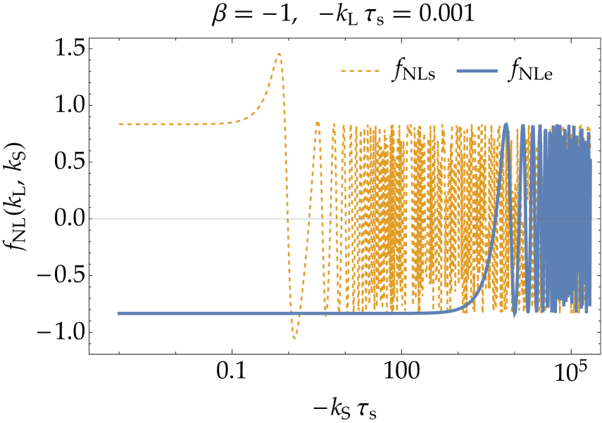
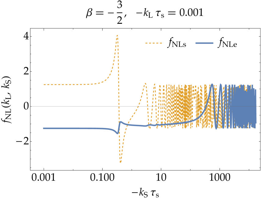
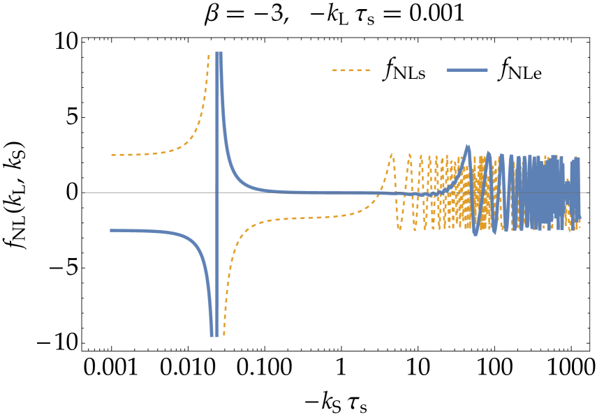
Figure 7: The bispectrum contributions from $\tau_{\mathrm{s}}$ (orange dashed) and $\tau_{\mathrm{e}}$ (blue) in terms of the generalized non-linearity parameter $f_{\mathrm{NL}}(k_{\mathrm{L}},k_{\mathrm{S}})$ (3.4) evaluated at sufficiently late time $\tau\to 0$ for $\beta=-1$ (top-left), $-3/2$ (top-right), and $-3$ (bottom) with $k_{\mathrm{L}}=-0.001/\tau_{\mathrm{s}}$.

In Fig. 8, we compare the non-linearity parameter with the spectral index for the short-wavelength mode:

$$n_{\mathrm{s}}(k_{\mathrm{S}})-1=\derivative{\ln\mathcal{P}_{\zeta}(k_{\mathrm{S}})}{\ln k_{\mathrm{S}}}.$$ (3.39)

One finds that for a sufficiently long-wavelength mode $-k_{\mathrm{L}}\tau_{\mathrm{s}}\ll 1$ which exits the horizon well before the onset of the constant-roll phase, Maldacena’s consistency relation

$$f_{\mathrm{NL}}(k_{\mathrm{L}},k_{\mathrm{S}})\underset{\text{CR}}{=}\frac{5}{12}\quantity(1-n_{\mathrm{s}}(k_{\mathrm{S}})),$$ (3.40)

holds well for any value of $\beta$ and for any short-wavelength mode $k_{\mathrm{S}}$ either on superhorizon or subhorizon scales at the end of the constant-roll phase. This result is consistent with the intuition: as $\zeta_{k_{\mathrm{L}}}$ is well frozen after exiting the horizon (even during or after the constant-roll phase), the logic developed in Sec. 3.1 can be applied and $\zeta_{k_{\mathrm{L}}}$ is merely viewed as a (comoving) scale shift by the short-wavelength modes. Physics in each local patch cannot distinguish $\zeta_{k_{\mathrm{L}}}$. PBHs produced in this model will hence show no spatial modulation beyond the adiabatic perturbation on a large scale [103].

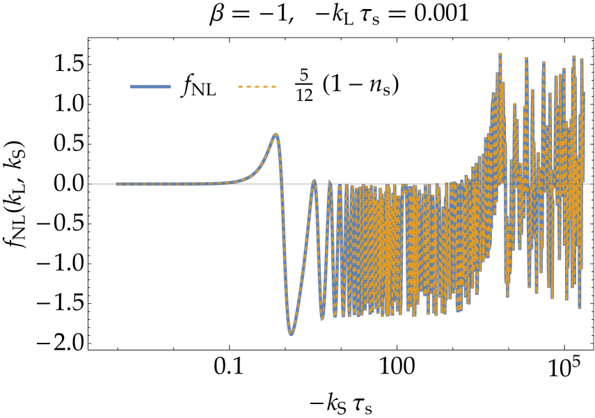
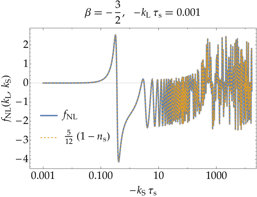
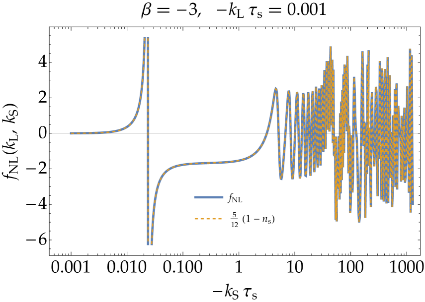
Figure 8: The total non-linearity parameter $f_{\mathrm{NL}}(k_{\mathrm{L}},k_{\mathrm{S}})$ with $k_{\mathrm{L}}=-0.001/\tau_{\mathrm{s}}$ (blue) and the spectral index $\frac{5}{12}\quantity(1-n_{\mathrm{s}}(k_{\mathrm{S}}))$ (orange dashed) evaluated at sufficiently late time $\tau\to 0$ for $\beta=-1$ (top-left), $-3/2$ (top-right), and $-3$ (bottom). For every model, Maldacena’s consistency relation (3.40) holds well.

On the other hand, for modes around the peak scale $\sim-1/\tau_{\mathrm{e}}$, violations of the consistency relation can be found for the non-attractor model $\beta\leq-3/2$ as shown in Fig. 9. This is because the curvature perturbation grows even on a superhorizon scale for the non-attractor model and it cannot be simply renormalized into the local scale factor. The peak-scale curvature perturbation itself is hence non-Gaussian and the PBH abundance is expected to be affected. The practical computation of these bispectra is done by the mode function with the Bunch–Davies initial condition set during the constant-roll phase, neglecting the $\tau_{\mathrm{s}}$ contribution, because all relevant modes are well subhorizon at $\tau_{\mathrm{s}}$.

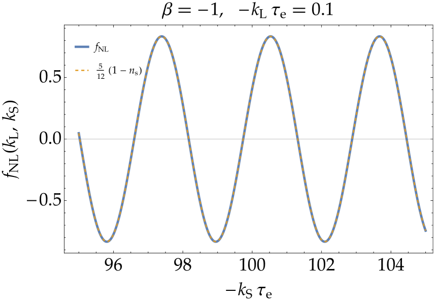
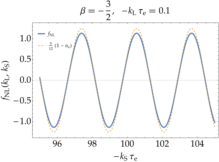
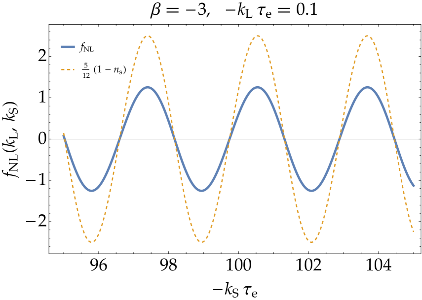
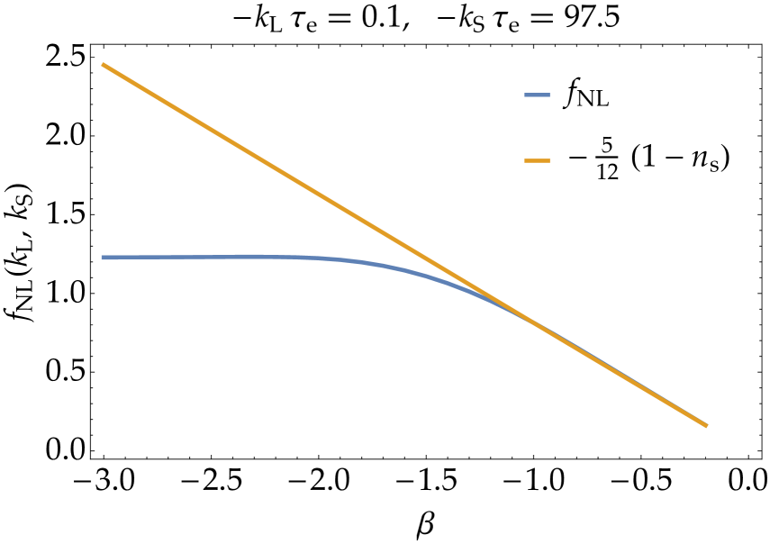
Figure 9: The similar plots to Fig. 8 but for $k_{\mathrm{L}}=-0.1/\tau_{\mathrm{e}}$ (top and bottom-left). The bottom-right panel compares $f_{\mathrm{NL}}$ and $-5(1-n_{\mathrm{s}})/12$ for $k_{\mathrm{S}}=-97.5/\tau_{\mathrm{e}}$, which shows the violation of Maldacena’s consistency relation for the non-attractor model $\beta\leq-3/2$.

3.4 Bispectrum during the constant-roll phase

Let us also discuss the bispectrum evaluated during the constant-roll phase though it does not directly affect the PBH physics. Boundary terms cannot be neglected in this case. In addition to the bulk contribution Fig. 6, two diagrams shown in Fig. 10 contribute, which we call the $\eta$-boundary and $H$-boundary terms, respectively (recall that the equal-time retarded propagator for the same operators vanishes for the $\eta$-boundary term). In terms of the non-linearity parameter, they read

$$f_{\mathrm{NL}\eta}=-\frac{5}{12}\times 4ia^{2}\epsilon\eta G_{\mathrm{c}\bar{\Delta}}(\tau,\tau;k_{\mathrm{S}})=\frac{5}{12}\eta,$$ (3.41)

$$f_{\mathrm{NL}H}=-\frac{5}{12}\times 8i\frac{a\epsilon}{H}\frac{G_{\mathrm{c}\bar{\Delta}}(\tau,\tau;k_{\mathrm{S}})G_{\mathrm{c}\bar{\mathrm{c}}}(\tau,\tau;k_{\mathrm{S}})}{P_{\zeta}(k_{\mathrm{S}})}=\frac{5}{6}\frac{{\rm Re}\,[\zeta_{k_{\mathrm{S}}}\zeta_{k_{\mathrm{S}}}^{*\prime}]}{aHP_{\zeta}(k_{\mathrm{S}})},$$

where we used the Wronskian condition $G_{\mathrm{c}\bar{\Delta}}(\tau,\tau;k)=i/(4a^{2}\epsilon)$. These contributions are equivalent to the redefinition contributions in Eq. (3.22) when using the $\zeta_{\mathrm{n}}$ approach as pointed out in Ref. [107]. In Fig. 11, we exemplify these contributions. They are indeed non-negligible compared to the bulk vertex contribution $f_{\mathrm{NLs}}$. Fig. 12 shows that the total bispectrum satisfies Maldacena’s consistency relation for a sufficiently long mode $k_{\mathrm{L}}$ even during the constant-roll phase as expected because such a long mode is frozen enough even at the onset of the constant-roll phase. Therefore, the boundary terms in the cubic action in terms of $\zeta$ are necessary for the realization of Maldacena’s consistency relation.

Figure 10: Two additional contributions from the boundary terms.

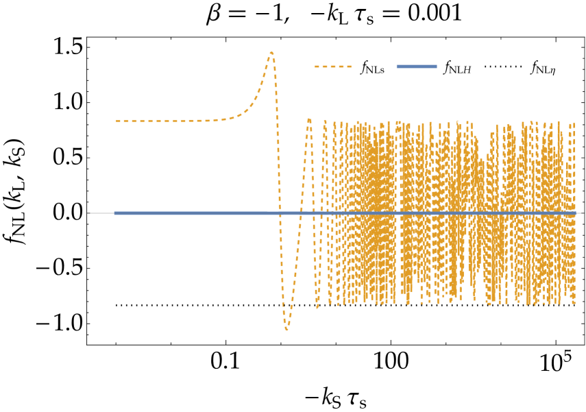
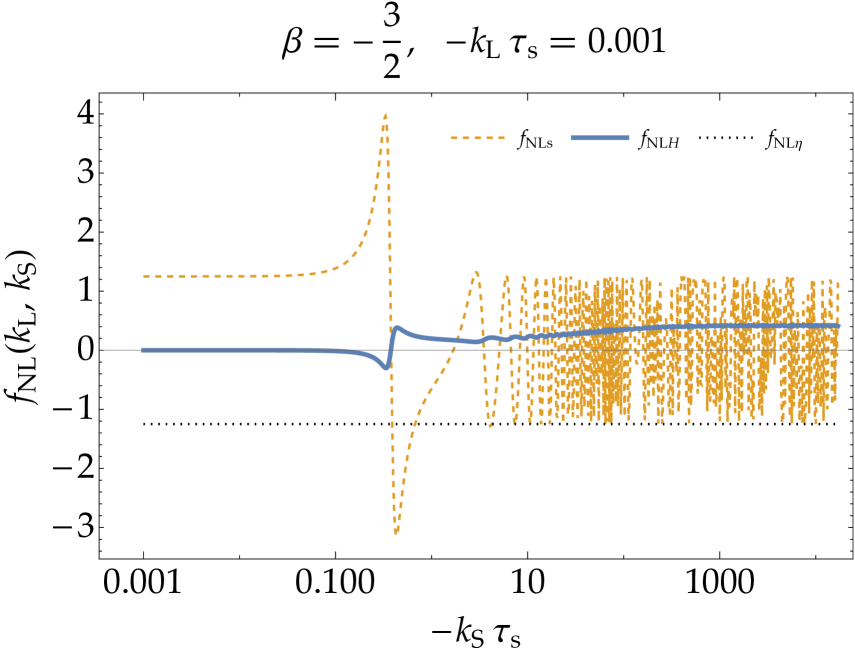
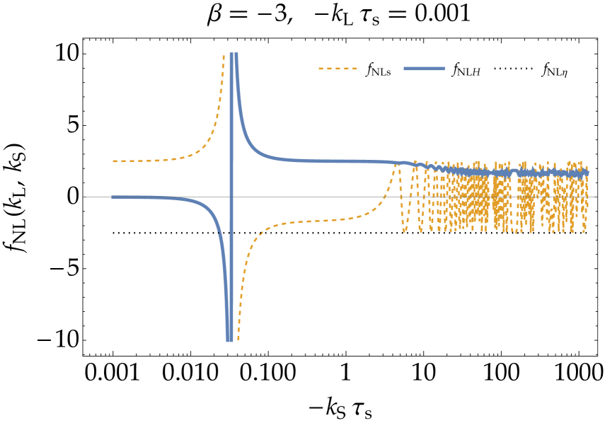
Figure 11: The bispectrum contributions from the bulk vertex at $\tau_{\mathrm{s}}$ (orange dashed), the $H$-boundary (blue), and $\eta$-boundary vertices (black dotted) evaluated during the constant-roll phase ($\tau\to\tau_{\mathrm{e}}-0$) for $\beta=-1$ (top-left), $-3/2$ (top-right), and $-3$ (bottom) with $k_{\mathrm{L}}=-0.001/\tau_{\mathrm{s}}$.

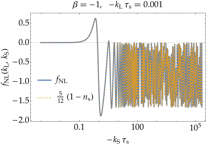
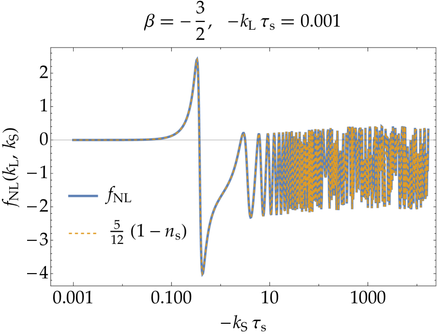
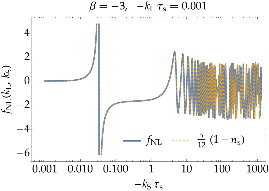
Figure 12: The total non-linearity parameter $f_{\mathrm{NL}}(k_{\mathrm{L}},k_{\mathrm{S}})$ with $k_{\mathrm{L}}=-0.001/\tau_{\mathrm{s}}$ (blue) and the spectral index $\frac{5}{12}\quantity(1-n_{\mathrm{s}}(k_{\mathrm{S}}))$ (orange dashed) evaluated during the constant-roll phase ($\tau\to\tau_{\mathrm{e}}-0$) for $\beta=-1$ (top-left), $-3/2$ (top-right), and $-3$ (bottom). Maldacena’s consistency relation (3.40) again holds well for every model thanks to the boundary terms.

4 One-loop correction to the long-wavelength mode

After elaborating on the squeezed bispectrum, now we are interested in the one-loop corrections in the transient constant-roll inflation. To evaluate the one-loop contributions, it is necessary to take into account all relevant terms carefully, which is beyond the scope of the present paper. In this section, as a preliminary step, we focus on one-loop terms evaluated in Ref. [73] for the ultra slow-roll scenario and clarify how the estimation is modified for a more general constant-roll scenario. We shall see that the PBH production in the transient constant-roll inflation is not prohibited from the perturbativity requirement on those one-loop terms.

Following Ref. [73], we calculate the one-loop correction to the power spectrum at $\tau_{\mathrm{e}}$ and the CMB pivot scale $k_{*}=$0.05\text{\,}\mathrm{M}\mathrm{p}\mathrm{c}^{-1}$$ originating from the $\dot{\eta}$ term in $S^{(3)}_{\mathrm{bulk}}$ in Eq. (LABEL:eq:_three_S3) at the instantaneous transition $\tau=\tau_{\mathrm{e}}$ by using the field redefinition $\zeta\to\zeta_{\mathrm{n}}$ given in Eq. (3.20) in the ordinary in-in formalism. Before the computation, let us analytically solve the junction condition (2.11), making use of the asymptotic expansion of the Hankel functions [123]

$$\lim_{z\to\infty}H^{(1/2)}_{\nu}(z)\approx\sqrt{\frac{2}{\pi z}}\mathrm{e}^{\pm i\left(z-\frac{\pi}{4}(2\nu+1)\right)}\left(1\pm\frac{ib}{z}\right),$$ (4.1)

$$\lim_{z\to 0}H^{(1/2)}_{\nu}(z)\approx\mp\frac{i}{\pi}\Gamma(\nu)\left(\frac{z}{2}\right)^{-\nu},$$ (4.2)

where

$$b=\frac{4\nu^{2}-1}{8}.$$ (4.3)

The curvature perturbation on subhorizon scales during the constant-roll phase follows Eq. (4.1) as

$$\zeta_{k}^{\mathrm{UV}}=\frac{iH}{2M_{\mathrm{Pl}}\sqrt{\epsilon_{\mathrm{SR}1}}}\frac{1}{k^{3/2}}F(k,\tau),$$ (4.4)

where

$$F(k,\tau)=\left(\frac{\tau_{\mathrm{s}}}{\tau}\right)^{\beta}\left[-\mathcal{A}_{k}(b+ik\tau)\mathrm{e}^{-i(k\tau+\pi(2\nu+1)/4)}+\mathcal{B}_{k}(b-ik\tau)\mathrm{e}^{i(k\tau+\pi(2\nu+1)/4)}\right].$$ (4.5)

Here and henceforth, $\nu$ and $b$ denote ${\nu_{\rm CR}}$ and $b_{\rm CR}$ for simplicity. The connection at $\tau_{\mathrm{s}}$ deep inside the horizon is solved as

$$\mathcal{A}_{k}=\frac{i\beta b-(\beta+1)(b-1)k\tau_{\mathrm{s}}+i(\beta-2b+2)k^{2}\tau_{\mathrm{s}}^{2}-2k^{3}\tau_{\mathrm{s}}^{3}}{2k\tau_{\mathrm{s}}[b(b-1)+k^{2}\tau_{\mathrm{s}}^{2}]}\mathrm{e}^{i\pi(2\nu+1)/4},$$ (4.6)

$$\mathcal{B}_{k}=\frac{-i\beta b+(\beta b+\beta-b+1)k\tau_{\mathrm{s}}+i\beta k^{2}\tau_{\mathrm{s}}^{2}}{2k\tau_{\mathrm{s}}[b(b-1)+k^{2}\tau_{\mathrm{s}}^{2}]}\mathrm{e}^{-i(\pi(2\nu-3)/4+2k\tau_{\mathrm{s}})}.$$

Using Eq. (4.2), the power spectrum at $\tau_{\mathrm{e}}$, $\mathcal{P}_{\mathrm{CR}}(k)$, is amplified from the first slow-roll phase solution $\mathcal{P}_{\mathrm{SR}}$ as

$$\mathcal{P}_{\mathrm{CR}}(k)=\mathcal{P}_{\mathrm{SR}}(k_{\mathrm{s}})\absolutevalue{F(k,\tau_{\mathrm{e}})}^{2}=\left(\frac{k_{\mathrm{s}}}{k_{*}}\right)^{-0.03}\mathcal{P}_{\mathrm{SR}}(k_{*})|F(k,\tau_{\mathrm{e}})|^{2}.$$ (4.7)

Here, we assumed that $\mathcal{P}_{\mathrm{SR}}$ is almost constant for $k\in[k_{\mathrm{s}}=-\tau_{\mathrm{s}}^{-1},k_{\mathrm{e}}=-\tau_{\mathrm{e}}^{-1}]$ but introduced a factor difference $\left(k_{\mathrm{s}}/k_{*}\right)^{-0.03}$ between $k_{\mathrm{s}}$ and $k_{*}$.

The one-loop correction $\mathcal{P}_{(1)}$ evaluated in Ref. [73] is generalized to

$$\mathcal{P}_{(1)}(k_{*})=\frac{1}{4}(\Delta\eta)^{2}\mathcal{P}_{\mathrm{SR}}^{2}(k_{*})\left(\frac{k_{\mathrm{s}}}{k_{*}}\right)^{-0.03}\int_{k_{\mathrm{s}}}^{k_{\mathrm{e}}}\frac{\differential{k}}{k}|F(k,\tau_{\mathrm{e}})|^{2},$$ (4.8)

where $\Delta\eta=-2\beta$ at $\tau=\tau_{\mathrm{e}}$, and the factor $\left(k_{\mathrm{s}}/k_{*}\right)^{-0.03}$ was introduced in (4.7). Here, the integral

$$I\equiv\int_{k_{\mathrm{s}}}^{k_{\mathrm{e}}}\frac{\differential{k}}{k}|F(k,\tau_{\mathrm{e}})|^{2}=\int_{1}^{\ell_{\mathrm{e}}}\frac{\differential{\ell}}{\ell}|F(\ell k_{\mathrm{s}},\tau_{\mathrm{e}})|^{2},$$ (4.9)

can be evaluated numerically, and the result is a function of $\ell_{\mathrm{e}}\equiv k_{\mathrm{e}}/k_{\mathrm{s}}$ for given $\beta$. An analytic form under the assumption $k_{\mathrm{e}}/k_{\mathrm{s}}\gg 1$ is given by

$$I\simeq\left(\frac{k_{\mathrm{e}}}{k_{\mathrm{s}}}\right)^{-2\beta}\left(c_{0}+c_{1}\ln\frac{k_{\mathrm{e}}}{k_{\mathrm{s}}}\right),$$ (4.10)

where

$$c_{0}=\begin{multlined}\frac{1}{2}+\frac{1}{120}\beta(\beta+1)^{2}(\beta+2)^{2}\left[\frac{5}{16}(5\beta^{5}+24\beta^{4}+44\beta^{3}+72\beta^{2}+143\beta+72)\right.\\ -\frac{1}{8}(12\beta^{5}+58\beta^{4}+65\beta^{3}+48\beta^{2}+101\beta+36)\cos 2\\ \left.+\frac{1}{2}(7\beta^{4}+24\beta^{3}+27\beta^{2}+26\beta-4)\sin 2\right],\end{multlined}\frac{1}{2}+\frac{1}{120}\beta(\beta+1)^{2}(\beta+2)^{2}\left[\frac{5}{16}(5\beta^{5}+24\beta^{4}+44\beta^{3}+72\beta^{2}+143\beta+72)\right.\\ -\frac{1}{8}(12\beta^{5}+58\beta^{4}+65\beta^{3}+48\beta^{2}+101\beta+36)\cos 2\\ \left.+\frac{1}{2}(7\beta^{4}+24\beta^{3}+27\beta^{2}+26\beta-4)\sin 2\right],$$ (4.11)

$$c_{1}=\frac{1}{4}(\beta+1)^{2}(\beta+2)^{2}.$$

We provide a derivation of the expression (4.10) and a comparison with numerical calculation in Appendix B.

As stressed above, in this section we focus only on $\mathcal{P}_{(1)}$ from the bulk interaction only at $\tau_{\mathrm{e}}$ and do not discuss whether other one-loop terms yield non-negligible contributions. Provided that this gives the dominant contribution, the perturbativity requires

$$\frac{\mathcal{P}_{(1)}(k_{*})}{\mathcal{P}_{\mathrm{SR}}(k_{*})}=\frac{1}{4}(\Delta\eta)^{2}\mathcal{P}_{\mathrm{SR}}(k_{*})\left(\frac{k_{\mathrm{e}}}{k_{*}}\right)^{-0.03}\left(\frac{k_{\mathrm{e}}}{k_{\mathrm{s}}}\right)^{0.03}I\left(\frac{k_{\mathrm{e}}}{k_{\mathrm{s}}}\right)\ll 1.$$ (4.12)

Here, $\mathcal{P}_{\mathrm{SR}}=2.1\times 10^{-9}$ and $\Delta\eta=-2\beta$. We adopt $k_{\mathrm{e}}$ as the PBH scale since it corresponds to the wavenumber for the peak of the power spectrum in the transient constant roll scenario as shown in Fig. 1. We consider two cases: the case of the PBH as dark matter with $k_{\mathrm{e}}=\mathcal{O}(10^{14})\,$\mathrm{M}\mathrm{p}\mathrm{c}^{-1}$$, and the LIGO–Virgo–KAGRA black holes with $k_{\mathrm{e}}=\mathcal{O}(10^{6})\,$\mathrm{M}\mathrm{p}\mathrm{c}^{-1}$$. For a given $k_{\mathrm{e}}$, the perturbativity requirement (4.12) yields an upper bound on $k_{\mathrm{e}}/k_{\mathrm{s}}$:

$$\frac{k_{\mathrm{e}}}{k_{\mathrm{s}}}\ll\ell_{\mathrm{crit}}.$$ (4.13)

We numerically evaluate the critical value $\ell_{\mathrm{crit}}$ for specific values of $\beta$ and $k_{\mathrm{e}}$ as follows. First, we substitute the analytic approximation (4.10) of the integral into (4.12) neglecting $\ln k_{\mathrm{e}}/k_{\mathrm{s}}$ in (4.10) and $\left(k_{\mathrm{e}}/k_{*}\right)^{-0.03}$ in (4.12) and analytically derive an approximated form of the critical value. Using this value as an initial guess, we perform a numerical root-finding algorithm with the analytic approximation (4.10) without neglecting $\ln k_{\mathrm{e}}/k_{\mathrm{s}}$ and $\left(k_{\mathrm{e}}/k_{*}\right)^{-0.03}$. Finally, using the root obtained in the second step as an initial guess, we perform a numerical root-finding algorithm with the integral $I$ numerically evaluated without approximation and obtain the critical value $\ell_{\mathrm{crit}}$. The fractional error between the root obtained in the second step and the critical value $\ell_{\mathrm{crit}}$ remains $\mathcal{O}(10^{-2})$ for $-3\leq\beta\lesssim-0.7$ but reaches $\mathcal{O}(10^{-1})$ for $\beta\geq-0.7$ so the final step is important.

In the left panel of Fig. 13, we represent the critical value $\ell_{\mathrm{crit}}$ as a function of $\beta$ for the two cases with $k_{\mathrm{e}}=10^{14}\,$\mathrm{M}\mathrm{p}\mathrm{c}^{-1}$$ and $10^{6}\,$\mathrm{M}\mathrm{p}\mathrm{c}^{-1}$$. For the ultra slow-roll case with $\beta=-3$, we obtain $\ell_{\mathrm{crit}}\simeq 18$ and $17$ for the two cases. In contrast, larger values are not prohibited for $\ell_{\mathrm{crit}}$ for general constant-roll models. It implies that a larger wavenumber range of the amplification of the power spectrum is compatible with the perturbativity requirement. We also see that the critical value $\ell_{\mathrm{crit}}$ is not sensitive to $k_{\mathrm{e}}$.

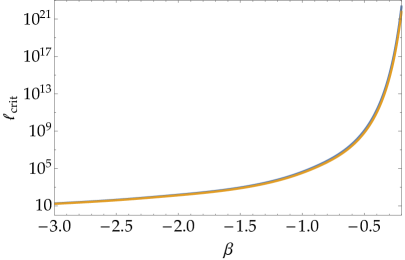
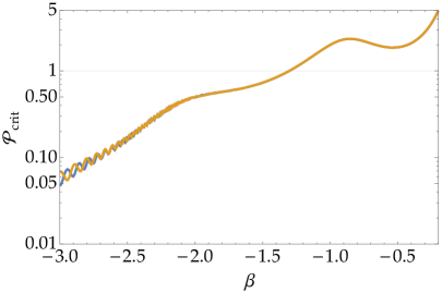
Figure 13: The critical values $\ell_{\mathrm{crit}}$ and $\mathcal{P}_{\mathrm{crit}}$ from the perturbativity requirement (see Eqs. (4.13) and (4.14)) for $k_{\mathrm{e}}=10^{14}\,$\mathrm{M}\mathrm{p}\mathrm{c}^{-1}$$ (blue) and $10^{6}\,$\mathrm{M}\mathrm{p}\mathrm{c}^{-1}$$ (orange).

The upper bound of $k_{\mathrm{e}}/k_{\mathrm{s}}$ puts a constraint on the power spectrum on PBH scales as

$$\mathcal{P}_{\rm PBH}\ll\mathcal{P}_{\mathrm{crit}},$$ (4.14)

where from Eq. (4.7) the critical value for the power spectrum is given by

$$\mathcal{P}_{\mathrm{crit}}\equiv\evaluated{\left(\frac{k_{\mathrm{s}}}{k_{*}}\right)^{-0.03}\mathcal{P}_{\mathrm{SR}}(k_{*})\absolutevalue{F(k_{\mathrm{e}},\tau_{\mathrm{e}})}^{2}}_{k_{\mathrm{e}}/k_{\mathrm{s}}=\ell_{\mathrm{crit}}}.$$ (4.15)

In the right panel of Fig. 13, we depict the critical value $\mathcal{P}_{\mathrm{crit}}$ for $k_{\mathrm{e}}=10^{14}\,$\mathrm{M}\mathrm{p}\mathrm{c}^{-1}$$ and $10^{6}\,$\mathrm{M}\mathrm{p}\mathrm{c}^{-1}$$. While there are small oscillations with respect to the values of $\beta$, the critical value $\mathcal{P}_{\mathrm{crit}}$ is not so sensitive to $k_{\mathrm{e}}$. As expected, while $\mathcal{P}_{\mathrm{crit}}\sim\mathcal{O}(10^{-2})$ for the transient ultra slow-roll scenario with $\beta=-3$, larger values are allowed for the transient constant-roll scenario. In particular, for the parameter range $-3/2<\beta<0$, where the constant-roll inflation is an attractor, $\mathcal{P}_{\mathrm{crit}}\gtrsim\mathcal{O}(1)$. Note that PBHs can be formed when $\mathcal{P}_{\rm PBH}\gtrsim\mathcal{O}(10^{-2})$, which is roughly two orders of magnitude below the critical value $\mathcal{P}_{\mathrm{crit}}$. Hence, the perturbativity requirement on the one-loop contribution $\mathcal{P}_{(1)}(k_{*})$ does not rule out the PBH production in the transient constant-roll inflation.

5 Conclusions

In canonical single-field inflation, the PBH production requires a transient violation of slow-roll. The representative scenario that satisfies the condition is the transient ultra slow-roll inflation, which has been extensively explored recently. More generally, we can consider the transient constant-roll inflation, where the power spectrum can be enhanced in non-/attractor inflationary dynamics. In the present paper, we investigated the squeezed bispectrum in the transient constant-roll inflation and also demonstrated how the one-loop corrections are modified from the transient ultra slow-roll inflation, picking up the representative terms originating from $\dot{\eta}$ term in the cubic action, as the first step to the full investigation of the one-loop analysis.

Applying the Feynman rule in the Schwinger–Keldysh formalism, we calculated the squeezed bispectrum both after and during the constant-roll phase. We confirmed that the Maldacena’s consistency relation holds for the bispectrum between the CMB scale mode and the PBH scale mode and hence the PBH distribution is not modulated beyond the adiabatic perturbation on large scales. On the other hand, for the non-attractor model, the bispectrum between the PBH scale modes themselves violates Maldacena’s consistency relation. Therefore, the detailed prediction of the PBH abundance, its clustering behaviour on small scales, or the corresponding induced GW requires special care to take into account the effects of the violation of the consistency relation.

We investigated the one-loop corrections originating from the $\dot{\eta}$ term in the cubic action in the transient constant-roll inflation and addressed whether the perturbativity requirement on those terms rules out the PBH production. We clarified that, compared to the transient ultra slow-roll inflation, a larger wavenumber range is allowed for the amplification of the power spectrum, and hence a larger amplification is allowed. As a result, we found that the PBH production is not ruled out from the perturbativity requirement, for both mass scales of the PBH as dark matter or LIGO–Virgo–KAGRA black holes.

Recently, the one-loop corrections in the PBH production from the transient ultra slow-roll inflation [73, 74, 75, 76, 77, 78, 79, 80, 81] and the resonance model [124] have been extensively explored, and it has been actively debated whether the perturbativity requirement rules out the PBH production in canonical single-field inflation. Our results show that the PBH production from the transient constant-roll inflation is not prohibited from the perturbativity requirement at least on the one-loop corrections originating from $\dot{\eta}$ term in the cubic action. However, we reiterate that in the present paper, we focused on particular terms of the one-loop corrections, which are often regarded as a dominant term in the literature. Other one-loop terms may or may not contribute in the transient constant-roll inflation. It requires a careful study to take into account all the relevant one-loop terms, which we leave for future work.

Appendix A Reconstruction of the step-function-like transition

In this appendix, we explicitly reconstruct a potential that realizes the step-function-like transition, which we consider in the main text:

$$\eta=\partial_{N}\ln\epsilon=\begin{cases}0,&\tau<\tau_{\mathrm{s}},\\ 2\beta,&\tau_{\mathrm{s}}\leq\tau<\tau_{\mathrm{e}},\\ 0,&\tau_{\mathrm{e}}\leq\tau,\end{cases}$$ (A.1)

with transition times $\tau_{\mathrm{s}}<\tau_{\mathrm{e}}$, the constant-roll parameter $\beta$, and the first slow-roll parameter $\epsilon=-\partial_{N}\ln H$. First, it is solved as

$$\ln\epsilon(N)=\int_{0}^{N}\eta\differential{N}+\ln\epsilon_{\mathrm{i}}=\begin{cases}\ln\epsilon_{\mathrm{i}},&N<N_{\mathrm{s}},\\ 2\beta(N-N_{\mathrm{s}})+\ln\epsilon_{\mathrm{i}},&N_{\mathrm{s}}\leq N<N_{\mathrm{e}},\\ 2\beta(N_{\mathrm{e}}-N_{\mathrm{s}})+\ln\epsilon_{\mathrm{i}},&N_{\mathrm{e}}\leq N,\end{cases}$$

$$\Rightarrow{} \epsilon(N)=\begin{cases}\epsilon_{\mathrm{i}},&N<N_{\mathrm{s}},\\ \epsilon_{\mathrm{i}}\mathrm{e}^{2\beta(N-N_{\mathrm{s}})},&N_{\mathrm{s}}\leq N<N_{\mathrm{e}},\\ \epsilon_{\mathrm{i}}\mathrm{e}^{2\beta(N_{\mathrm{e}}-N_{\mathrm{s}})},&N_{\mathrm{e}}\leq N,\end{cases}$$ (A.2)

where $\epsilon_{\mathrm{i}}$ is the initial value of $\epsilon$ at the initial time which we choose $N=0$ without loss of generality. $N_{\mathrm{s}}$ and $N_{\mathrm{e}}$ are e-folding times corresponding to $\tau_{\mathrm{s}}$ and $\tau_{\mathrm{e}}$, respectively. As $\epsilon$ is also related to the inflaton’s velocity by $\epsilon=\frac{1}{2}\pqty{\derivative{\phi}{N}}^{2}$, if one assumes $\derivative*{\phi}{N}>0$ without loss of generality, it is solved as

$$\derivative{\phi}{N}=\sqrt{2\epsilon}=\begin{cases}\sqrt{2\epsilon_{\mathrm{i}}},&N<N_{\mathrm{s}},\\ \sqrt{2\epsilon_{\mathrm{i}}}\mathrm{e}^{\beta(N-N_{\mathrm{s}})},&N_{\mathrm{s}}\leq N<N_{\mathrm{e}},\\ \sqrt{2\epsilon_{\mathrm{i}}}\mathrm{e}^{\beta(N_{\mathrm{e}}-N_{\mathrm{s}})},&N_{\mathrm{e}}\leq N,\end{cases}$$

$$\Rightarrow{} \phi(N)=\begin{cases}\sqrt{2\epsilon_{\mathrm{i}}}N,&N<N_{\mathrm{s}},\\ \sqrt{2\epsilon_{\mathrm{i}}}\bqty{\frac{1}{\beta}\pqty{\mathrm{e}^{\beta(N-N_{\mathrm{s}})}-1}+N_{\mathrm{s}}},&N_{\mathrm{s}}\leq N<N_{\mathrm{e}},\\ \sqrt{2\epsilon_{\mathrm{i}}}\bqty{\mathrm{e}^{\beta(N_{\mathrm{e}}-N_{\mathrm{s}})}(N-N_{\mathrm{e}})+\frac{1}{\beta}\pqty{\mathrm{e}^{\beta(N_{\mathrm{e}}-N_{\mathrm{s}})}-1}+N_{\mathrm{s}}},&N_{\mathrm{e}}\leq N,\end{cases}$$ (A.3)

where we set the initial field value $\phi(N=0)=0$ without loss of generality. Its inverse function is found as

$$N(\phi)=\begin{cases}\frac{\phi}{\sqrt{2\epsilon_{\mathrm{i}}}},&\phi<\phi_{\mathrm{s}},\\ N_{\mathrm{s}}+\frac{1}{\beta}\ln\bqty{\beta\pqty{\frac{\phi}{\sqrt{2\epsilon_{\mathrm{i}}}}-N_{\mathrm{s}}}+1},&\phi_{\mathrm{s}}\leq\phi<\phi_{\mathrm{e}},\\ N_{\mathrm{e}}+\mathrm{e}^{-\beta(N_{\mathrm{e}}-N_{\mathrm{s}})}\bqty{\frac{\phi}{\sqrt{2\epsilon_{\mathrm{i}}}}-\frac{1}{\beta}\pqty{\mathrm{e}^{\beta(N_{\mathrm{e}}-N_{\mathrm{s}})}-1}-N_{\mathrm{s}}},&\phi_{\mathrm{e}}\leq\phi,\end{cases}$$ (A.4)

where $\phi_{\mathrm{s}}=\phi(N_{\mathrm{s}})$ and $\phi_{\mathrm{e}}=\phi(N_{\mathrm{e}})$. $\epsilon$ is further related to the Hubble parameter by $\epsilon=-\partial_{N}\ln H$, which means

$$\ln H(N)=\begin{cases}\ln H_{\mathrm{i}}-\epsilon_{\mathrm{i}}N,&N<N_{\mathrm{s}},\\ \ln H_{\mathrm{i}}-\frac{\epsilon_{\mathrm{i}}}{2\beta}\pqty{\mathrm{e}^{2\beta(N-N_{\mathrm{s}})}-1}-\epsilon_{\mathrm{i}}N_{\mathrm{s}},&N_{\mathrm{s}}\leq N<N_{\mathrm{e}},\\ \ln H_{\mathrm{i}}-\epsilon_{\mathrm{i}}\mathrm{e}^{2\beta(N_{\mathrm{e}}-N_{\mathrm{s}})}(N-N_{\mathrm{e}})-\frac{\epsilon_{\mathrm{i}}}{2\beta}\pqty{\mathrm{e}^{2\beta(N_{\mathrm{e}}-N_{\mathrm{s}})}-1}-\epsilon_{\mathrm{i}}N_{\mathrm{s}},&N_{\mathrm{e}}\leq N,\end{cases}$$

$$\Rightarrow{} H(N)=\begin{cases}H_{\mathrm{i}}\mathrm{e}^{-\epsilon_{\mathrm{i}}N},&N<N_{\mathrm{s}},\\ H_{\mathrm{i}}\exp\bqty{-\frac{\epsilon_{\mathrm{i}}}{2\beta}\pqty{\mathrm{e}^{2\beta(N-N_{\mathrm{s}})}-1}-\epsilon_{\mathrm{i}}N_{\mathrm{s}}},&N_{\mathrm{s}}\leq N<N_{\mathrm{e}},\\ H_{\mathrm{i}}\exp\bqty{-\epsilon_{\mathrm{i}}\mathrm{e}^{2\beta(N_{\mathrm{e}}-N_{\mathrm{s}})}(N-N_{\mathrm{e}})-\frac{\epsilon_{\mathrm{i}}}{2\beta}\pqty{\mathrm{e}^{2\beta(N_{\mathrm{e}}-N_{\mathrm{s}})}-1}-\epsilon_{\mathrm{i}}N_{\mathrm{s}}},&N_{\mathrm{e}}\leq N,\end{cases}$$ (A.5)

where $H_{\mathrm{i}}$ is the initial value of the Hubble parameter. Combining it with Eq. (A.4), one finds $H$ as a function of $\phi$ as

$$H(\phi)=\begin{cases}H_{\mathrm{i}}\mathrm{e}^{-\sqrt{\frac{\epsilon_{\mathrm{i}}}{2}}\phi},&\phi<\phi_{\mathrm{s}},\\ H_{\mathrm{i}}\exp\bqty{-\frac{\epsilon_{\mathrm{i}}\beta}{2}\pqty{\frac{\phi}{\sqrt{2\epsilon_{\mathrm{i}}}}-N_{\mathrm{s}}}^{2}-\sqrt{\frac{\epsilon_{\mathrm{i}}}{2}}\phi},&\phi_{\mathrm{s}}\leq\phi<\phi_{\mathrm{e}},\\[10.0pt] \begin{multlined}\textstyle H_{\mathrm{i}}\exp\left[-\epsilon_{\mathrm{i}}\mathrm{e}^{\beta(N_{\mathrm{e}}-N_{\mathrm{s}})}\pqty{\frac{\phi}{\sqrt{2\epsilon_{\mathrm{i}}}}-\frac{1}{\beta}\pqty{\mathrm{e}^{\beta(N_{\mathrm{e}}-N_{\mathrm{s}})}-1}-N_{\mathrm{s}}}\right.\\[-10.0pt] \textstyle\left.-\frac{\epsilon_{\mathrm{i}}}{2\beta}\pqty{\mathrm{e}^{2\beta(N_{\mathrm{e}}-N_{\mathrm{s}})}-1}-\epsilon_{\mathrm{i}}N_{\mathrm{s}}\right],\end{multlined}\textstyle H_{\mathrm{i}}\exp\left[-\epsilon_{\mathrm{i}}\mathrm{e}^{\beta(N_{\mathrm{e}}-N_{\mathrm{s}})}\pqty{\frac{\phi}{\sqrt{2\epsilon_{\mathrm{i}}}}-\frac{1}{\beta}\pqty{\mathrm{e}^{\beta(N_{\mathrm{e}}-N_{\mathrm{s}})}-1}-N_{\mathrm{s}}}\right.\\[-10.0pt] \textstyle\left.-\frac{\epsilon_{\mathrm{i}}}{2\beta}\pqty{\mathrm{e}^{2\beta(N_{\mathrm{e}}-N_{\mathrm{s}})}-1}-\epsilon_{\mathrm{i}}N_{\mathrm{s}}\right],&\phi_{\mathrm{e}}\leq\phi.\end{cases}$$ (A.6)

The Hamilton–Jacobi equation finally connects the Hubble parameter to the potential by

$$V(\phi) =3H^{2}(\phi)-2{H^{\prime}(\phi)}^{2}$$

$$=\begin{cases}(3-\epsilon_{\mathrm{i}})H_{\mathrm{i}}^{2}\mathrm{e}^{-\sqrt{2\epsilon_{\mathrm{i}}}\phi},&\phi<\phi_{\mathrm{s}},\\[5.0pt] \begin{multlined}\textstyle-\frac{1}{2}H_{\mathrm{i}}^{2}\left[\beta^{2}\phi^{2}-2\sqrt{2\epsilon_{\mathrm{i}}}\beta\phi(\beta N_{\mathrm{s}}-1)+2\epsilon_{\mathrm{i}}(\beta N_{\mathrm{s}}-1)^{2}-6\right]\\[-10.0pt] \textstyle\times\exp\left[-\frac{1}{2}\phi\left(\beta\phi+2\sqrt{2\epsilon_{\mathrm{i}}}\right)-\beta N_{\mathrm{s}}^{2}\epsilon_{\mathrm{i}}+\sqrt{2\epsilon_{\mathrm{i}}}\beta N_{\mathrm{s}}\phi\right],\end{multlined}\textstyle-\frac{1}{2}H_{\mathrm{i}}^{2}\left[\beta^{2}\phi^{2}-2\sqrt{2\epsilon_{\mathrm{i}}}\beta\phi(\beta N_{\mathrm{s}}-1)+2\epsilon_{\mathrm{i}}(\beta N_{\mathrm{s}}-1)^{2}-6\right]\\[-10.0pt] \textstyle\times\exp\left[-\frac{1}{2}\phi\left(\beta\phi+2\sqrt{2\epsilon_{\mathrm{i}}}\right)-\beta N_{\mathrm{s}}^{2}\epsilon_{\mathrm{i}}+\sqrt{2\epsilon_{\mathrm{i}}}\beta N_{\mathrm{s}}\phi\right],&\phi_{\mathrm{s}}\leq\phi<\phi_{\mathrm{e}},\\[5.0pt] \begin{multlined}\textstyle\left(3-\epsilon_{\mathrm{i}}\mathrm{e}^{2\beta(N_{\mathrm{e}}-N_{\mathrm{s}})}\right)H_{\mathrm{i}}^{2}\\[-10.0pt] \textstyle\times\exp\left(\frac{\epsilon_{\mathrm{i}}\left(\mathrm{e}^{\beta(N_{\mathrm{e}}-N_{\mathrm{s}})}-1\right)\left(\mathrm{e}^{\beta(N_{\mathrm{e}}-N_{\mathrm{s}})}+2\beta N_{\mathrm{s}}-1\right)}{\beta}-\sqrt{2\epsilon_{\mathrm{i}}}\phi\mathrm{e}^{\beta(N_{\mathrm{e}}-N_{\mathrm{s}})}\right),\end{multlined}\textstyle\left(3-\epsilon_{\mathrm{i}}\mathrm{e}^{2\beta(N_{\mathrm{e}}-N_{\mathrm{s}})}\right)H_{\mathrm{i}}^{2}\\[-10.0pt] \textstyle\times\exp\left(\frac{\epsilon_{\mathrm{i}}\left(\mathrm{e}^{\beta(N_{\mathrm{e}}-N_{\mathrm{s}})}-1\right)\left(\mathrm{e}^{\beta(N_{\mathrm{e}}-N_{\mathrm{s}})}+2\beta N_{\mathrm{s}}-1\right)}{\beta}-\sqrt{2\epsilon_{\mathrm{i}}}\phi\mathrm{e}^{\beta(N_{\mathrm{e}}-N_{\mathrm{s}})}\right),&\phi_{\mathrm{e}}\leq\phi.\end{cases}$$ (A.7)

For this potential, one can numerically solve the inflaton’s dynamics through its equation of motion

$$\ddot{\phi}+3H\dot{\phi}+V^{\prime}(\phi)=0,\quad 3H^{2}=\frac{\dot{\phi}^{2}}{2}+V(\phi),$$ (A.8)

and reproduce the step-function-like transition (A.1) as shown in Fig. 14.

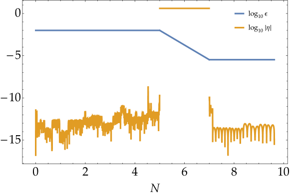
Figure 14: Numerical results of the slow-roll parameters $\log_{10}\epsilon$ (blue) and $\log_{10}\absolutevalue{\eta}$ (orange) for the inflarinary dynamics with the reconstructed potential (A) with the parameter set $\beta=-2$, $\epsilon_{\mathrm{i}}=10^{-2}$, $H_{\mathrm{i}}=10^{-5}$, $N_{\mathrm{s}}=5$, and $N_{\mathrm{e}}=7$. The noisy feature of $\eta$ would be caused by the numerical error.

Appendix B Evaluation of the integral (4.9)

In this appendix, we analytically evaluate the integral (4.9) under the assumption $\ell_{\mathrm{e}}\equiv k_{\mathrm{e}}/k_{\mathrm{s}}\gg 1$ and derive the approximated form (4.10). For $k\simeq k_{\mathrm{e}}$, the function $F(k_{\mathrm{e}},\tau_{\mathrm{e}})$ in the integrand scales as $|F(k_{\mathrm{e}},\tau_{\mathrm{e}})|^{2}\simeq\ell_{\mathrm{e}}^{-2\beta}(\beta^{4}+6\beta^{3}+13\beta^{2}+12\beta+8)/4$ for $\ell_{\mathrm{e}}\gg 1$. Below we shall consider an approximation for $k_{\mathrm{s}}\leq k\leq k_{\mathrm{e}}$.

First, we decompose the integrand into the nonoscillating part $G_{1}(\ell)$ and oscillating part $G_{2}(\ell)$:

$$\frac{|F(\ell k_{\mathrm{s}},\tau_{\mathrm{e}})|^{2}}{\ell}=G_{1}(\ell)+G_{2}(\ell)+G_{2}^{*}(\ell),$$ (B.1)

where

$$G_{1}(\ell)=\begin{multlined}\frac{\ell_{\mathrm{e}}^{-2(\beta+1)}}{2\ell^{3}[\ell^{2}+b(b-1)]^{2}}(\ell^{2}+b^{2}\ell_{\mathrm{e}}^{2})\\ \times[2\ell^{6}+\left(\beta^{2}+2b(b-1)\right)\ell^{4}+\left(b^{2}(\beta-1)^{2}+(\beta+1)^{2}-2b\right)\ell^{2}+b^{2}\beta^{2}],\end{multlined}\frac{\ell_{\mathrm{e}}^{-2(\beta+1)}}{2\ell^{3}[\ell^{2}+b(b-1)]^{2}}(\ell^{2}+b^{2}\ell_{\mathrm{e}}^{2})\\ \times[2\ell^{6}+\left(\beta^{2}+2b(b-1)\right)\ell^{4}+\left(b^{2}(\beta-1)^{2}+(\beta+1)^{2}-2b\right)\ell^{2}+b^{2}\beta^{2}],$$ (B.2)

$$G_{2}(\ell)=\begin{multlined}\frac{i\ell_{\mathrm{e}}^{-2(\beta+1)}\mathrm{e}^{-2i\ell(1-1/\ell_{\mathrm{e}})}}{4\ell^{3}[\ell^{2}+b(b-1)]^{2}}(\ell+ib\ell_{\mathrm{e}})^{2}[\beta\ell^{2}-i(b(\beta-1)+\beta+1)\ell-b\beta]\\ \times[2\ell^{3}+i(-2b+\beta+2)\ell^{2}+(b-1)(\beta+1)\ell+ib\beta].\end{multlined}\frac{i\ell_{\mathrm{e}}^{-2(\beta+1)}\mathrm{e}^{-2i\ell(1-1/\ell_{\mathrm{e}})}}{4\ell^{3}[\ell^{2}+b(b-1)]^{2}}(\ell+ib\ell_{\mathrm{e}})^{2}[\beta\ell^{2}-i(b(\beta-1)+\beta+1)\ell-b\beta]\\ \times[2\ell^{3}+i(-2b+\beta+2)\ell^{2}+(b-1)(\beta+1)\ell+ib\beta].$$

Since $|b(b-1)|\leq 1/4$ for $-3<\beta<0$, we approximate $\ell^{2}+b(b-1)\simeq\ell^{2}$ in the denominator of $G_{1}$ and $G_{2}$.

For the nonoscillating part, we simply integrate it, pick up terms with the highest power of $\ell_{\mathrm{e}}$, and arrive at

$$I_{1} \equiv\int_{1}^{\ell_{\mathrm{e}}}G_{1}(\ell)\differential{\ell}$$

$$\begin{multlined}\simeq\ell_{\mathrm{e}}^{-2\beta}\left[\frac{1}{4}(\beta+1)^{2}(\beta+2)^{2}\ln\ell_{\mathrm{e}}+\frac{1}{2}\right.\\ \left.+\frac{1}{384}\beta(\beta+1)^{2}(\beta+2)^{2}\left(5\beta^{5}+24\beta^{4}+44\beta^{3}+72\beta^{2}+143\beta+72\right)\right].\end{multlined}\simeq\ell_{\mathrm{e}}^{-2\beta}\left[\frac{1}{4}(\beta+1)^{2}(\beta+2)^{2}\ln\ell_{\mathrm{e}}+\frac{1}{2}\right.\\ \left.+\frac{1}{384}\beta(\beta+1)^{2}(\beta+2)^{2}\left(5\beta^{5}+24\beta^{4}+44\beta^{3}+72\beta^{2}+143\beta+72\right)\right].$$ (B.5)

The nonoscillating part yields the dominant contribution.

For the oscillating part, the contribution to the integral mainly comes from $\ell\sim 1$ since $G_{2}$ is rapidly oscillating with a slowly varying envelope, and hence the contribution to the integral is negligible for $\ell\gg 1$. Hence, we Taylor expand the integrand around $\ell=1$ up to the first order, integrate it, and then pick up terms with the highest power of $\ell_{\mathrm{e}}$. As a result, we obtain

$$I_{2} \equiv\int_{1}^{\ell_{\mathrm{e}}}[G_{2}(\ell)+G_{2}^{*}(\ell)]\differential{\ell}$$

$$\begin{multlined}\simeq\frac{\ell_{\mathrm{e}}^{-2\beta}}{960}\beta(\beta+1)^{2}(\beta+2)^{2}\left[4\left(7\beta^{4}+24\beta^{3}+27\beta^{2}+26\beta-4\right)\sin 2\right.\\ \left.-\left(12\beta^{5}+58\beta^{4}+65\beta^{3}+48\beta^{2}+101\beta+36\right)\cos 2\right].\end{multlined}\simeq\frac{\ell_{\mathrm{e}}^{-2\beta}}{960}\beta(\beta+1)^{2}(\beta+2)^{2}\left[4\left(7\beta^{4}+24\beta^{3}+27\beta^{2}+26\beta-4\right)\sin 2\right.\\ \left.-\left(12\beta^{5}+58\beta^{4}+65\beta^{3}+48\beta^{2}+101\beta+36\right)\cos 2\right].$$ (B.8)

With these results, we obtain the analytic approximation of the integral $I=I_{1}+I_{2}$ as in (4.10). One can recover the result $\left(\frac{k_{\mathrm{e}}}{k_{\mathrm{s}}}\right)^{6}\left(1.1+\ln\frac{k_{\mathrm{e}}}{k_{\mathrm{s}}}\right)$ obtained in Ref. [73] by substituting $\beta=-3$. In Fig. 15, we compare the analytic formula and numerical calculation for the parameter range $-3<\beta<0$, and confirm that they are in good agreement.

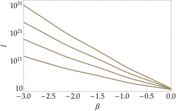
Figure 15: The integral $I$ as a function of the constant roll parameter $\beta$. Numerical integration of the exact form (4.9) (blue, solid) and the approximation (4.10) (orange, dashed) are shown for $\ell_{\mathrm{e}}\equiv k_{\mathrm{e}}/k_{\mathrm{s}}=10^{2}$, $10^{3}$, $10^{4}$, and $10^{5}$ (from bottom to top).

References

- [1] Y. B. Zel’dovich and I. D. Novikov, The Hypothesis of Cores Retarded during Expansion and the Hot Cosmological Model, Soviet Astron. AJ (Engl. Transl. ), 10 (1967) 602.
- [2] S. Hawking, Gravitationally collapsed objects of very low mass, Mon. Not. Roy. Astron. Soc. 152 (1971) 75.
- [3] B. J. Carr and S. W. Hawking, Black holes in the early Universe, Mon. Not. Roy. Astron. Soc. 168 (1974) 399.
- [4] B. J. Carr, The Primordial black hole mass spectrum, Astrophys. J. 201 (1975) 1.
- [5] B. Carr, K. Kohri, Y. Sendouda and J. Yokoyama, Constraints on primordial black holes, Rept. Prog. Phys. 84 (2021) 116902 [2002.12778].
- [6] M. Sasaki, T. Suyama, T. Tanaka and S. Yokoyama, Primordial black holes—perspectives in gravitational wave astronomy, Class. Quant. Grav. 35 (2018) 063001 [1801.05235].
- [7] H. Niikura, M. Takada, S. Yokoyama, T. Sumi and S. Masaki, Constraints on Earth-mass primordial black holes from OGLE 5-year microlensing events, Phys. Rev. D 99 (2019) 083503 [1901.07120].
- [8] P. D. Serpico, V. Poulin, D. Inman and K. Kohri, Cosmic microwave background bounds on primordial black holes including dark matter halo accretion, Phys. Rev. Res. 2 (2020) 023204 [2002.10771].
- [9] B. Carr and J. Silk, Primordial Black Holes as Generators of Cosmic Structures, Mon. Not. Roy. Astron. Soc. 478 (2018) 3756 [1801.00672].
- [10] B. Liu and V. Bromm, Accelerating Early Massive Galaxy Formation with Primordial Black Holes, Astrophys. J. Lett. 937 (2022) L30 [2208.13178].
- [11] A. Escrivà, F. Kuhnel and Y. Tada, Primordial Black Holes, 2211.05767.
- [12] H. Motohashi and W. Hu, Primordial Black Holes and Slow-Roll Violation, Phys. Rev. D 96 (2017) 063503 [1706.06784].
- [13] N. Tsamis and R. P. Woodard, Improved estimates of cosmological perturbations, Phys.Rev. D69 (2004) 084005 [astro-ph/0307463].
- [14] W. H. Kinney, Horizon crossing and inflation with large eta, Phys.Rev. D72 (2005) 023515 [gr-qc/0503017].
- [15] J. Garcia-Bellido and E. Ruiz Morales, Primordial black holes from single field models of inflation, Phys. Dark Univ. 18 (2017) 47 [1702.03901].
- [16] J. M. Ezquiaga, J. Garcia-Bellido and E. Ruiz Morales, Primordial Black Hole production in Critical Higgs Inflation, Phys. Lett. B 776 (2018) 345 [1705.04861].
- [17] C. Germani and T. Prokopec, On primordial black holes from an inflection point, Phys. Dark Univ. 18 (2017) 6 [1706.04226].
- [18] G. Ballesteros and M. Taoso, Primordial black hole dark matter from single field inflation, Phys. Rev. D 97 (2018) 023501 [1709.05565].
- [19] M. Cicoli, V. A. Diaz and F. G. Pedro, Primordial Black Holes from String Inflation, JCAP 06 (2018) 034 [1803.02837].
- [20] M. Biagetti, G. Franciolini, A. Kehagias and A. Riotto, Primordial Black Holes from Inflation and Quantum Diffusion, JCAP 07 (2018) 032 [1804.07124].
- [21] I. Dalianis, A. Kehagias and G. Tringas, Primordial black holes from -attractors, JCAP 01 (2019) 037 [1805.09483].
- [22] C. T. Byrnes, P. S. Cole and S. P. Patil, Steepest growth of the power spectrum and primordial black holes, JCAP 06 (2019) 028 [1811.11158].
- [23] S. Passaglia, W. Hu and H. Motohashi, Primordial black holes and local non-Gaussianity in canonical inflation, Phys. Rev. D 99 (2019) 043536 [1812.08243].
- [24] N. Bhaumik and R. K. Jain, Primordial black holes dark matter from inflection point models of inflation and the effects of reheating, JCAP 01 (2020) 037 [1907.04125].
- [25] D. Y. Cheong, S. M. Lee and S. C. Park, Primordial black holes in Higgs- inflation as the whole of dark matter, JCAP 01 (2021) 032 [1912.12032].
- [26] H. V. Ragavendra, P. Saha, L. Sriramkumar and J. Silk, Primordial black holes and secondary gravitational waves from ultraslow roll and punctuated inflation, Phys. Rev. D 103 (2021) 083510 [2008.12202].
- [27] D. G. Figueroa, S. Raatikainen, S. Rasanen and E. Tomberg, Non-Gaussian Tail of the Curvature Perturbation in Stochastic Ultraslow-Roll Inflation: Implications for Primordial Black Hole Production, Phys. Rev. Lett. 127 (2021) 101302 [2012.06551].
- [28] C. Pattison, V. Vennin, D. Wands and H. Assadullahi, Ultra-slow-roll inflation with quantum diffusion, JCAP 04 (2021) 080 [2101.05741].
- [29] K. Inomata, E. McDonough and W. Hu, Primordial black holes arise when the inflaton falls, Phys. Rev. D 104 (2021) 123553 [2104.03972].
- [30] K. Inomata, E. McDonough and W. Hu, Amplification of primordial perturbations from the rise or fall of the inflaton, JCAP 02 (2022) 031 [2110.14641].
- [31] S. R. Geller, W. Qin, E. McDonough and D. I. Kaiser, Primordial black holes from multifield inflation with nonminimal couplings, Phys. Rev. D 106 (2022) 063535 [2205.04471].
- [32] J. Martin, H. Motohashi and T. Suyama, Ultra Slow-Roll Inflation and the non-Gaussianity Consistency Relation, Phys. Rev. D 87 (2013) 023514 [1211.0083].
- [33] H. Motohashi, A. A. Starobinsky and J. Yokoyama, Inflation with a constant rate of roll, JCAP 09 (2015) 018 [1411.5021].
- [34] H. Motohashi and A. A. Starobinsky, constant-roll inflation, Eur. Phys. J. C 77 (2017) 538 [1704.08188].
- [35] H. Motohashi and A. A. Starobinsky, Constant-roll inflation in scalar-tensor gravity, JCAP 11 (2019) 025 [1909.10883].
- [36] H. Motohashi and A. A. Starobinsky, Constant-roll inflation: confrontation with recent observational data, EPL 117 (2017) 39001 [1702.05847].
- [37] J. T. Galvez Ghersi, A. Zucca and A. V. Frolov, Observational Constraints on Constant Roll Inflation, JCAP 1905 (2019) 030 [1808.01325].
- [38] N. K. Stein and W. H. Kinney, Simple single-field inflation models with arbitrarily small tensor/scalar ratio, JCAP 03 (2023) 027 [2210.05757].
- [39] H. Motohashi, S. Mukohyama and M. Oliosi, Constant Roll and Primordial Black Holes, JCAP 03 (2020) 002 [1910.13235].
- [40] S. S. Mishra and V. Sahni, Primordial Black Holes from a tiny bump/dip in the Inflaton potential, JCAP 04 (2020) 007 [1911.00057].
- [41] O. Özsoy and Z. Lalak, Primordial black holes as dark matter and gravitational waves from bumpy axion inflation, JCAP 01 (2021) 040 [2008.07549].
- [42] A. Karam, N. Koivunen, E. Tomberg, V. Vaskonen and H. Veermäe, Anatomy of single-field inflationary models for primordial black holes, JCAP 03 (2023) 013 [2205.13540].
- [43] J. S. Bullock and J. R. Primack, NonGaussian fluctuations and primordial black holes from inflation, Phys. Rev. D 55 (1997) 7423 [astro-ph/9611106].
- [44] P. Ivanov, Nonlinear metric perturbations and production of primordial black holes, Phys. Rev. D 57 (1998) 7145 [astro-ph/9708224].
- [45] J. Yokoyama, Chaotic new inflation and formation of primordial black holes, Phys. Rev. D 58 (1998) 083510 [astro-ph/9802357].
- [46] J. C. Hidalgo, The effect of non-Gaussian curvature perturbations on the formation of primordial black holes, 0708.3875.
- [47] C. T. Byrnes, E. J. Copeland and A. M. Green, Primordial black holes as a tool for constraining non-Gaussianity, Phys. Rev. D 86 (2012) 043512 [1206.4188].
- [48] E. V. Bugaev and P. A. Klimai, Primordial black hole constraints for curvaton models with predicted large non-Gaussianity, Int. J. Mod. Phys. D 22 (2013) 1350034 [1303.3146].
- [49] S. Young, D. Regan and C. T. Byrnes, Influence of large local and non-local bispectra on primordial black hole abundance, JCAP 02 (2016) 029 [1512.07224].
- [50] T. Nakama, J. Silk and M. Kamionkowski, Stochastic gravitational waves associated with the formation of primordial black holes, Phys. Rev. D 95 (2017) 043511 [1612.06264].
- [51] K. Ando, K. Inomata, M. Kawasaki, K. Mukaida and T. T. Yanagida, Primordial black holes for the LIGO events in the axionlike curvaton model, Phys. Rev. D 97 (2018) 123512 [1711.08956].
- [52] G. Franciolini, A. Kehagias, S. Matarrese and A. Riotto, Primordial Black Holes from Inflation and non-Gaussianity, JCAP 03 (2018) 016 [1801.09415].
- [53] V. Atal and C. Germani, The role of non-gaussianities in Primordial Black Hole formation, Phys. Dark Univ. 24 (2019) 100275 [1811.07857].
- [54] V. Atal, J. Garriga and A. Marcos-Caballero, Primordial black hole formation with non-Gaussian curvature perturbations, JCAP 09 (2019) 073 [1905.13202].
- [55] V. Atal, J. Cid, A. Escrivà and J. Garriga, PBH in single field inflation: the effect of shape dispersion and non-Gaussianities, JCAP 05 (2020) 022 [1908.11357].
- [56] C.-M. Yoo, J.-O. Gong and S. Yokoyama, Abundance of primordial black holes with local non-Gaussianity in peak theory, JCAP 09 (2019) 033 [1906.06790].
- [57] M. Taoso and A. Urbano, Non-gaussianities for primordial black hole formation, JCAP 08 (2021) 016 [2102.03610].
- [58] N. Kitajima, Y. Tada, S. Yokoyama and C.-M. Yoo, Primordial black holes in peak theory with a non-Gaussian tail, JCAP 10 (2021) 053 [2109.00791].
- [59] A. Escrivà, Y. Tada, S. Yokoyama and C.-M. Yoo, Simulation of primordial black holes with large negative non-Gaussianity, JCAP 05 (2022) 012 [2202.01028].
- [60] J. R. Chisholm, Clustering of primordial black holes: basic results, Phys. Rev. D 73 (2006) 083504 [astro-ph/0509141].
- [61] S. Young, C. T. Byrnes and M. Sasaki, Calculating the mass fraction of primordial black holes, JCAP 1407 (2014) 045 [1405.7023].
- [62] S. Young and C. T. Byrnes, Long-short wavelength mode coupling tightens primordial black hole constraints, Phys. Rev. D 91 (2015) 083521 [1411.4620].
- [63] Y. Tada and S. Yokoyama, Primordial black holes as biased tracers, Phys. Rev. D 91 (2015) 123534 [1502.01124].
- [64] S. Young and C. T. Byrnes, Signatures of non-gaussianity in the isocurvature modes of primordial black hole dark matter, JCAP 04 (2015) 034 [1503.01505].
- [65] T. Suyama and S. Yokoyama, Clustering of primordial black holes with non-Gaussian initial fluctuations, PTEP 2019 (2019) 103E02 [1906.04958].
- [66] S. Young and C. T. Byrnes, Initial clustering and the primordial black hole merger rate, JCAP 03 (2020) 004 [1910.06077].
- [67] R.-g. Cai, S. Pi and M. Sasaki, Gravitational Waves Induced by non-Gaussian Scalar Perturbations, Phys. Rev. Lett. 122 (2019) 201101 [1810.11000].
- [68] C. Unal, Imprints of Primordial Non-Gaussianity on Gravitational Wave Spectrum, Phys. Rev. D 99 (2019) 041301 [1811.09151].
- [69] C. Yuan and Q.-G. Huang, Gravitational waves induced by the local-type non-Gaussian curvature perturbations, Phys. Lett. B 821 (2021) 136606 [2007.10686].
- [70] P. Adshead, K. D. Lozanov and Z. J. Weiner, Non-Gaussianity and the induced gravitational wave background, JCAP 10 (2021) 080 [2105.01659].
- [71] K. T. Abe, R. Inui, Y. Tada and S. Yokoyama, Primordial black holes and gravitational waves induced by exponential-tailed perturbations, 2209.13891.
- [72] G. Domènech, Scalar Induced Gravitational Waves Review, Universe 7 (2021) 398 [2109.01398].
- [73] J. Kristiano and J. Yokoyama, Ruling Out Primordial Black Hole Formation From Single-Field Inflation, 2211.03395.
- [74] J. Kristiano and J. Yokoyama, Response to criticism on ”Ruling Out Primordial Black Hole Formation From Single-Field Inflation”: A note on bispectrum and one-loop correction in single-field inflation with primordial black hole formation, 2303.00341.
- [75] A. Riotto, The Primordial Black Hole Formation from Single-Field Inflation is Not Ruled Out, 2301.00599.
- [76] A. Riotto, The Primordial Black Hole Formation from Single-Field Inflation is Still Not Ruled Out, 2303.01727.
- [77] S. Choudhury, M. R. Gangopadhyay and M. Sami, No-go for the formation of heavy mass Primordial Black Holes in Single Field Inflation, 2301.10000.
- [78] S. Choudhury, S. Panda and M. Sami, No-go for PBH formation in EFT of single field inflation, 2302.05655.
- [79] S. Choudhury, S. Panda and M. Sami, Quantum loop effects on the power spectrum and constraints on primordial black holes, 2303.06066.
- [80] H. Firouzjahi, One-loop Corrections in Power Spectrum in Single Field Inflation, 2303.12025.
- [81] H. Firouzjahi and A. Riotto, Primordial Black Holes and Loops in Single-Field Inflation, 2304.07801.
- [82] J. M. Maldacena, Non-Gaussian features of primordial fluctuations in single field inflationary models, JHEP 05 (2003) 013 [astro-ph/0210603].
- [83] M. J. P. Morse and W. H. Kinney, Large- constant-roll inflation is never an attractor, Phys. Rev. D 97 (2018) 123519 [1804.01927].
- [84] Q. Gao, Y. Gong and Z. Yi, On the constant-roll inflation with large and small , Universe 5 (2019) 215 [1901.04646].
- [85] W.-C. Lin, M. J. P. Morse and W. H. Kinney, Dynamical Analysis of Attractor Behavior in Constant Roll Inflation, JCAP 09 (2019) 063 [1904.06289].
- [86] Planck collaboration, Y. Akrami et al., Planck 2018 results. X. Constraints on inflation, Astron. Astrophys. 641 (2020) A10 [1807.06211].
- [87] P. Creminelli and M. Zaldarriaga, Single field consistency relation for the 3-point function, JCAP 10 (2004) 006 [astro-ph/0407059].
- [88] X. Chen, M.-x. Huang and G. Shiu, The Inflationary Trispectrum for Models with Large Non-Gaussianities, Phys. Rev. D 74 (2006) 121301 [hep-th/0610235].
- [89] C. Cheung, A. L. Fitzpatrick, J. Kaplan and L. Senatore, On the consistency relation of the 3-point function in single field inflation, JCAP 02 (2008) 021 [0709.0295].
- [90] M. Li and Y. Wang, Consistency Relations for Non-Gaussianity, JCAP 09 (2008) 018 [0807.3058].
- [91] D. Seery, M. S. Sloth and F. Vernizzi, Inflationary trispectrum from graviton exchange, JCAP 03 (2009) 018 [0811.3934].
- [92] Y. Urakawa and T. Tanaka, Influence on observation from IR divergence during inflation: Multi field inflation, Prog. Theor. Phys. 122 (2010) 1207 [0904.4415].
- [93] L. Leblond and E. Pajer, Resonant Trispectrum and a Dozen More Primordial N-point functions, JCAP 01 (2011) 035 [1010.4565].
- [94] T. Tanaka and Y. Urakawa, Dominance of gauge artifact in the consistency relation for the primordial bispectrum, JCAP 05 (2011) 014 [1103.1251].
- [95] P. Creminelli, G. D’Amico, M. Musso and J. Norena, The (not so) squeezed limit of the primordial 3-point function, JCAP 11 (2011) 038 [1106.1462].
- [96] P. Creminelli, J. Noreña and M. Simonović, Conformal consistency relations for single-field inflation, JCAP 07 (2012) 052 [1203.4595].
- [97] K. Hinterbichler, L. Hui and J. Khoury, Conformal Symmetries of Adiabatic Modes in Cosmology, JCAP 08 (2012) 017 [1203.6351].
- [98] V. Assassi, D. Baumann and D. Green, On Soft Limits of Inflationary Correlation Functions, JCAP 11 (2012) 047 [1204.4207].
- [99] E. Pajer, F. Schmidt and M. Zaldarriaga, The Observed Squeezed Limit of Cosmological Three-Point Functions, Phys. Rev. D 88 (2013) 083502 [1305.0824].
- [100] Z. Kenton and D. J. Mulryne, The Separate Universe Approach to Soft Limits, JCAP 10 (2016) 035 [1605.03435].
- [101] Y. Tada and V. Vennin, Squeezed bispectrum in the formalism: local observer effect in field space, JCAP 02 (2017) 021 [1609.08876].
- [102] B. Finelli, G. Goon, E. Pajer and L. Santoni, Soft Theorems For Shift-Symmetric Cosmologies, Phys. Rev. D 97 (2018) 063531 [1711.03737].
- [103] T. Suyama, Y. Tada and M. Yamaguchi, Local observer effect on the cosmological soft theorem, PTEP 2020 (2020) 113E01 [2008.13364].
- [104] T. Suyama, Y. Tada and M. Yamaguchi, Revisiting non-Gaussianity in non-attractor inflation models in the light of the cosmological soft theorem, PTEP 2021 (2021) 073E02 [2101.10682].
- [105] G. L. Pimentel, L. Senatore and M. Zaldarriaga, On Loops in Inflation III: Time Independence of zeta in Single Clock Inflation, JHEP 07 (2012) 166 [1203.6651].
- [106] H. Collins, Primordial non-Gaussianities from inflation, 1101.1308.
- [107] F. Arroja and T. Tanaka, A note on the role of the boundary terms for the non-Gaussianity in general k-inflation, JCAP 05 (2011) 005 [1103.1102].
- [108] P. Adshead, W. Hu and V. Miranda, Bispectrum in Single-Field Inflation Beyond Slow-Roll, Phys. Rev. D 88 (2013) 023507 [1303.7004].
- [109] S. Passaglia and W. Hu, Scalar Bispectrum Beyond Slow-Roll in the Unified EFT of Inflation, Phys. Rev. D 98 (2018) 023526 [1804.07741].
- [110] A. Kamenev and A. Levchenko, Keldysh technique and non-linear -model: basic principles and applications, Advances in Physics 58 (2009) 197 [0901.3586].
- [111] E. Calzetta and B. L. Hu, Closed Time Path Functional Formalism in Curved Space-Time: Application to Cosmological Back Reaction Problems, Phys. Rev. D 35 (1987) 495.
- [112] N. C. Tsamis and R. P. Woodard, Quantum gravity slows inflation, Nucl. Phys. B 474 (1996) 235 [hep-ph/9602315].
- [113] N. C. Tsamis and R. P. Woodard, The Quantum gravitational back reaction on inflation, Annals Phys. 253 (1997) 1 [hep-ph/9602316].
- [114] S. Weinberg, Quantum contributions to cosmological correlations, Phys. Rev. D 72 (2005) 043514 [hep-th/0506236].
- [115] M. van der Meulen and J. Smit, Classical approximation to quantum cosmological correlations, JCAP 11 (2007) 023 [0707.0842].
- [116] D. Seery, One-loop corrections to a scalar field during inflation, JCAP 11 (2007) 025 [0707.3377].
- [117] T. Prokopec and G. Rigopoulos, Path Integral for Inflationary Perturbations, Phys. Rev. D 82 (2010) 023529 [1004.0882].
- [118] J.-O. Gong, M.-S. Seo and G. Shiu, Path integral for multi-field inflation, JHEP 07 (2016) 099 [1603.03689].
- [119] X. Chen, Y. Wang and Z.-Z. Xianyu, Loop Corrections to Standard Model Fields in Inflation, JHEP 08 (2016) 051 [1604.07841].
- [120] X. Chen, Y. Wang and Z.-Z. Xianyu, Schwinger-Keldysh Diagrammatics for Primordial Perturbations, JCAP 12 (2017) 006 [1703.10166].
- [121] J. Tokuda and T. Tanaka, Statistical nature of infrared dynamics on de Sitter background, JCAP 02 (2018) 014 [1708.01734].
- [122] J. Tokuda and T. Tanaka, Can all the infrared secular growth really be understood as increase of classical statistical variance?, JCAP 11 (2018) 022 [1806.03262].
- [123] “NIST Digital Library of Mathematical Functions.” https://dlmf.nist.gov/, Release 1.1.9 of 2023-03-15.
- [124] K. Inomata, M. Braglia and X. Chen, Questions on calculation of primordial power spectrum with large spikes: the resonance model case, 2211.02586.