Holography from lattice ${\cal N}=4$ super Yang-Mills

Abstract

In this paper we use lattice simulation to study four dimensional ${\cal N}=4$ super Yang-Mills (SYM) theory. We have focused on the three color theory on lattices of size $12^{4}$ and for ’t Hooft couplings up to $\lambda=40.0$. Our lattice action is based on a discretization of the Marcus or GL twist of ${\cal N}=4$ SYM and retains one exact supersymmetry for non-zero lattice spacing. We show that lattice theory exists in a single non-Abelian Coulomb phase for all ’t Hooft couplings. Furthermore the static potential we obtain from correlators of Polyakov lines is in good agreement with that obtained from holography - specifically the potential has a Coulombic form with a coefficent that varies as the square root of the ’t Hooft coupling.

1 Introduction

${\cal N}=4$ super Yang-Mills is both a fascinating and non-trivial quantum field theory. It possesses a line of conformal fixed points, is conjectured to be invariant under a strong-weak coupling duality, and most importantly, furnishes the original example of holographic duality by providing a description of type IIb string theory on five dimensional anti-de Sitter space. The holographic description is most easily understood in the planar $N_{c}\to\infty$ strong coupling limit where the five dimensional theory reduces to classical supergravity. However, string loop corrections arise at $O(\frac{1}{N_{c}})$ and are difficult to access analytically. This provides motivation to study the theory using numerical simulation.

Naive approaches to constructing a lattice theory break supersymmetry completely and lead to a large number of relevant supersymmetry breaking counterterms whose couplings would need to be tuned to take a continuum limit. This stymied progress for many years until models were constructed that preserved one or more supercharges at non-zero lattice spacing - see the review Catterall:2009it and references therein. The key idea underlying these constructions is to find linear combinations of the continuum supercharges that are nilpotent and hence compatible with finite lattice translations. This may be accomplished either by discretization of a topologically twisted version of the supersymmetric theory Catterall:2007kn or by building a lattice theory from a matrix model using orbifolding and deconstruction techniques Cohen:2003xe ; Cohen:2003qw ; Kaplan:2005ta .

While these developments have led to many numerical studies providing evidence supporting holography for dimensional reductions of ${\cal N}=4$ Yang-Mills Hanada:2016zxj ; Anagnostopoulos:2007fw ; Hanada:2008gy ; Catterall:2008yz ; Catterall:2009xn ; Catterall:2010fx ; Berkowitz:2016jlq ; Catterall:2017lub ; Rinaldi:2017mjl ; Catterall:2020nmn it has proven difficult until recently to test holography directly in four dimensions. The original supersymmetric construction in four dimensions produced lattice artifacts in the form of $U(1)$ monopoles that condense and lead to a chirally broken phase for ’t Hooft couplings $\lambda>4$ Catterall:2012yq ; Catterall:2014vka . Recently we have constructed a new lattice action that appears to avoid these problems Catterall:2020lsi . It differs from both the original and improved Catterall:2015ira actions for ${\cal N}=4$ SYM by the addition of a new supersymmetric term that breaks the gauge symmetry from $U(N)$ to $SU(N)$. This removes the monopoles completely and, as we will show in this paper, yields a single non-Abelian Coulomb phase.

2 Lattice action

We use the supersymmetric lattice action appearing in Catterall:2020lsi .

$$S=\frac{N}{4\lambda}{\cal Q}\sum_{x}{\rm Tr\;}\left[\chi_{ab}{\cal F}_{ab}+\eta\left({\overline{\cal D}}_{a}{\cal U}_{a}+\kappa\left({\rm Re\,det\,}{\cal U}_{a}(x)-1\right)I_{N}\right)+\frac{1}{2}\eta d\right]+S_{\rm closed}$$ (1)

where the lattice field strength

$${\cal F}_{ab}(x)={\cal U}_{a}(x){\cal U}_{b}(x+\hat{a})-{\cal U}_{b}(x){\cal U}_{a}(x+\hat{b})$$ (2)

where ${\cal U}_{a}(x)$ denotes the complexified gauge field living on the lattice link running from $x\to x+\hat{a}$ and $\hat{a}$ denotes one of the five basis vectors of an underlying $A_{4}^{*}$ lattice. $I_{N}$ denotes the $N\times N$ unit matrix in color space. Similarly

$${\overline{\cal D}}_{a}{\cal U}_{a}={\cal U}_{a}(x){\overline{\cal U}}_{a}(x)-{\overline{\cal U}}_{a}(x-\hat{a}){\cal U}_{a}(x-\hat{a}).$$ (3)

The five fermion fields $\psi_{a}$, being superpartners of the (complex) gauge fields, live on the corresponding links, while the ten fermion fields $\chi_{ab}(x)$ are associated with new face links running from $x+\hat{a}+\hat{b}\to x$. The scalar fermion $\eta(x)$ lives on the lattice site $x$ and is associated with a conserved supercharge ${\cal Q}$ which acts on the fields in the following way

$${\cal Q}\,{\cal U}_{a} \to\psi_{a}$$

$${\cal Q}\,\psi_{a} \to 0$$

$${\cal Q}\,\eta \to d$$

$${\cal Q}\,d \to 0$$

$${\cal Q}\,\chi_{ab} \to{\overline{\cal F}}_{ab}$$

$${\cal Q}\,{\overline{\cal U}}_{a} \to 0$$ (4)

Notice that ${\cal Q}^{2}=0$ which guarantees the supersymmetric invariance of the first part of the lattice action. The auxiliary site field $d(x)$ is needed for nilpotency of ${\cal Q}$ offshell. The second term $S_{\rm closed}$ is given by

$$S_{\rm closed}=-\frac{N}{16\lambda}\sum_{x}{\rm Tr\;}\epsilon_{abcde}\chi_{ab}{\overline{\cal D}}_{c}\chi_{de}$$ (5)

where the covariant difference operator acting on the fermion field $\chi_{de}$ takes the form

$${\overline{\cal D}}_{c}\chi_{de}(x)={\overline{\cal U}}_{c}(x-\hat{c})\chi_{de}(x+\hat{a}+\hat{b})-\chi_{de}(x-\hat{d}-\hat{e}){\overline{\cal U}}_{c}(x+\hat{a}+\hat{b})$$ (6)

The latter term can be shown to be supersymmetric via an exact lattice Bianchi identity $\epsilon_{abcde}{\overline{\cal D}}_{c}{\overline{\cal F}}_{de}=0$. Carrying out the ${\cal Q}$ variation and integrating out the auxiliary field $d$ we obtain the final supersymmetric lattice action $S=S_{b}+S_{f}$ where

$$S_{b}=\frac{N}{4\lambda}\sum_{x}{\rm Tr\;}\left({\cal F}_{ab}{\overline{\cal F}}_{ab}\right)+\frac{1}{2}{\rm Tr\;}({\overline{\cal D}}_{a}{\cal U}_{a}+\kappa({\rm Re\,det\,}{\cal U}_{a}-1)I_{N})^{2}$$ (7)

and

$$S_{f} =-\frac{N}{4\lambda}\sum_{x}\left({\rm Tr\;}\chi_{ab}{\cal D}_{\left[a\right.}\psi_{\left.b\right]}+{\rm Tr\;}\eta{\overline{\cal D}}_{a}\psi_{a}+\frac{1}{4}{\rm Tr\;}\epsilon_{abcde}\chi_{ab}{\overline{\cal D}}_{c}\chi_{de}\right)-$$ (8)

$$\frac{\kappa N}{8\lambda}\sum_{x,a}{\rm Tr\;}(\eta)\,{\rm det\,}{\cal U}_{a}(x){\rm Tr\;}({\cal U}_{a}^{-1}(x)\psi_{a}(x))$$ (9)

Setting $\kappa=0$ and taking the naive continuum limit ${\cal U}_{a}=I+{\cal A}_{a}+\ldots$ one can show that this action can be obtained by discretization of the Marcus or GL twist of ${\cal N}=4$ Yang-Mills in flat space Marcus:1995mq ; Kapustin:2006pk . In the continuum this twisted formulation is used to construct a topological field theory but here we use the twisted construction merely as a change of variables that allows for discretization while preserving the single exact supersymmetry ${\cal Q}$.

As described above, the discrete theory is defined on a somewhat exotic lattice - $A_{4}^{*}$. This admits a larger set of discrete rotational symmetries corresponding to the group $S^{5}$ in comparison to those of a hypercubic lattice and this fact plays a role in controlling the renormalization of the theory Catterall:2013roa . In fact one can show that gauge symmetry, ${\cal Q}$ supersymmetry and $S^{5}$ invariance ensure that the only relevant counterterms correspond to operators present in the classical lattice action together with a single new marginal operator of the form $\alpha\sum_{x,a}{\rm Tr}\,(\eta{\cal U}_{a}{\overline{\cal U}}_{a})$. However, the calculation in Catterall:2011pd shows that even this term is absent at $\kappa=0$ to all orders in perturbation theory.

Finally, to retain exact supersymmetry, all fields reside in the algebra of the gauge group – taking their values in the adjoint representation of $U(N)$: $f(x)=\sum_{A=1}^{N^{2}}T^{A}f^{A}(x)$ with ${\rm Tr\;}(T^{A}T^{B})=-\delta^{AB}$. Ordinarily this would be incompatible with lattice gauge invariance because the measure would not be gauge invariant for link based fields. However, in this ${\cal N}=4$ construction the problem is evaded since the fields are complexified which ensures that the Jacobians that arise after gauge transformation of ${\cal U}$ and ${\overline{\cal U}}$ cancel.

The term involving the coupling $\kappa$ suppresses the troublesome $U(1)$ modes while leaving the important $SU(N)$ gauge symmetry intact. It also has another advantage; by selecting out gauge fields with unit determinant it ensures that the gauge field has the expansion ${\cal U}_{a}(x)=I+{\cal A}_{a}(x)+\ldots$ where ${\cal A}_{a}$ are traceless complex fields. This ensures the correct naive continuum limit.

The resultant action still possesses a set of flat directions corresponding to constant gauge fields that are valued in the Cartan subalgebra. To regulate these flat directions we additionally add to the action a term of the form

$$S_{\rm mass}=\mu^{2}\sum_{x}{\rm Tr\;}\left({\overline{\cal U}}_{a}(x){\cal U}_{a}(x)-I\right)^{2}$$ (10)

While this breaks the exact supersymmetry softly all counter terms induced by this breaking will have couplings that are multiplicative in $\mu^{2}$ and hence vanishing as $\mu^{2}\to 0$.

3 Results

Our simulations utilize the rational hybrid Monte Carlo (HMC) algorithm where the Pfaffian resulting from the fermion integration is replaced by

$${\rm Pf}\,(M)={\rm det}\left[\left(M^{\dagger}M\right)^{\frac{1}{4}}\right]$$ (11)

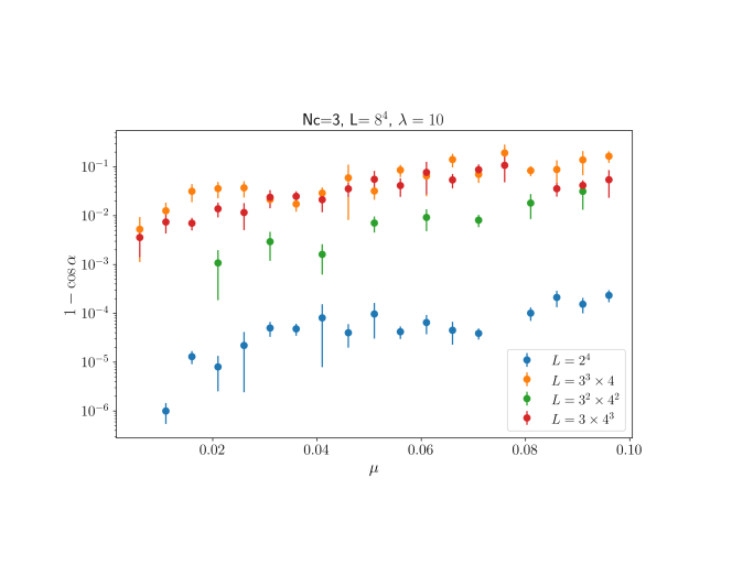
Figure 6: $1-cos(\alpha)$ vs $\mu$ for $L=2^{4},3^{3}\times 4,3^{2}\times 4^{2},4^{3}\times 3$

where $M$ is the fermion operator and the fractional power is replaced by a rational fraction approximation Clark:2006wq . In principle this throws away any phase in the fermion operator. In the appendix (fig. 6) we show that this phase is always small even at strong coupling for sufficiently small $\mu^{2}$. Typical ensembles used in our analysis consist of $3500-4000$ HMC trajectories with $750-800$ discarded for thermalization. Errors are assessed using a jackknife procedure using $20-40$ bins. We also fix $\kappa=1$ for all our simulations.

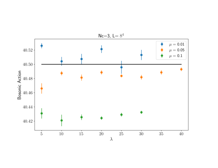
Figure 1: Bosonic Action vs $\lambda$ for $8^{4}$ lattice at $\kappa=1.0$ for various values of $\mu$

One of the simplest observables that can be measured is the expectation value of the bosonic action. This can be calculated exactly at any coupling by exploiting the exact lattice supersymmetry. We start by rescaling the fermions to remove the dependence of the ${\cal Q}$-closed term on $\beta=\frac{N}{4\lambda}$ so that the partition function $Z$ is given by

$$Z=\beta^{\frac{-6N^{2}V}{2}}\int D\eta D\psi D\chi DUD{\overline{\cal U}}Dd\;e^{-\beta{\cal Q}\Lambda-\chi{\overline{\cal D}}\chi}$$ (12)

where $\Lambda$ generates the ${\cal Q}$-exact terms in the action and $V$ is the number of lattice points. After integrating over the auxiliary field $d$ one finds that the coefficient $-\frac{6}{2}N^{2}V$ is shifted to $-\frac{7}{2}N^{2}V$. But

$$-\frac{\partial\ln{Z}}{\partial\beta}=<S_{B}>-<S_{F}>=-\frac{7N^{2}V}{2\beta}+<{\cal Q}\Lambda>$$ (13)

Using the ${\cal Q}$ Ward identity $<{\cal Q}\Lambda>=0$ and the fact that the expectation value of the fermion action can be trivially found by a scaling argument since the fermion fields appear only quadratically one finds the final result

$$\frac{1}{V}\beta S_{B}=\frac{9N^{2}}{2}$$ (14)

Fig.1 shows the bosonic action density as a function of $\lambda$ for several values of the susy breaking mass $\mu$. It should be clear that the measured values approach the exact result $<\beta\frac{S_{B}}{V}>=40.5$ independent of $\lambda$ as $\mu\to 0$.

To check that we have indeed suppressed the $U(1)$ modes we plot the expectation value of the link determinant in fig. 2. Clearly the observed value of the link determinant lies close to unity for all ’t Hooft couplings provided that $\mu$ is small enough. Notice that both the bosonic action and the link determinant show no sign of a phase transition over the range $0<\lambda<40$. This is consistent with the continuum expectation that the ${\cal N}=4$ SYM theory exists in a single phase out to arbitrarily strong coupling.

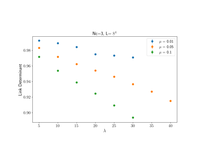
Figure 2: Link Determinant vs $\lambda$ for $8^{4}$ lattice and $\kappa=1.0$

The conclusion is strengthened further by examining a variety of supersymmetric Wilson loop corresponding to the product of complexified lattice gauge fields around a closed loop on the lattice. We have plotted the logarithm of such Wilson loops as a function of $\sqrt{\lambda}$ in fig. 3. Clearly the behavior is smooth as $\lambda$ varies and again there is no sign of any phase transition. Furthermore the linear dependence of $W$ seen for large $\lambda$ is consistent with holography. Indeed, both square and circular Wilson loops can be computed in the strong coupling planar limit and show a $\sqrt{\lambda}$ dependence on the ’t Hooft coupling Maldacena:1998im ; Drukker:2000rr .

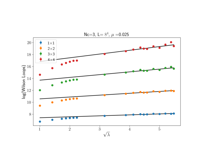
Figure 3: $R\times R$ Wilson Loops vs $\sqrt{\lambda}$ for $8^{4}$ lattices at $\mu=0.025$ and $\kappa=1.0$

It should be noted that this $\lambda$ dependence cannot be seen in perturbation theory and constitutes a non-trivial test that the lattice model is able to reproduce the non-perturbative physics of the continuum theory.

However fig. 3 makes it clear that there is also a perimeter dependence to the Wilson loop. This is not unexpected and arises also in the continuum calculations as a regulator term associated with a bare quark mass. In general the Wilson loop arises as the amplitude for the propagation of heavy fundamental sources that interact via a static potential of the form

$$V(r)=-\frac{\alpha}{r}+M$$ (15)

where $M$ represents the static quark mass. To subtract the perimeter term from our analysis and look for the presence of an underlying non-abelian Coulomb term in the static potential we have turned to another related observable – the correlation function of two Polyakov lines. These are just Wilson lines that close via the toroidal boundary conditions. The measured correlator is defined by

$$P(r)=\sum_{x,y}\left[<P(x)P^{\dagger}(y)>-<P(x)><P^{\dagger}(y)>\delta(r,|x-y|)\right]$$ (16)

where $|x-y|$ is the distance in the $A_{4}^{*}$ lattice. As for the Wilson loop it is expected to vary like

$$P(r)\sim e^{-V(r)t}$$ (17)

with $V(r)$ the static potential.

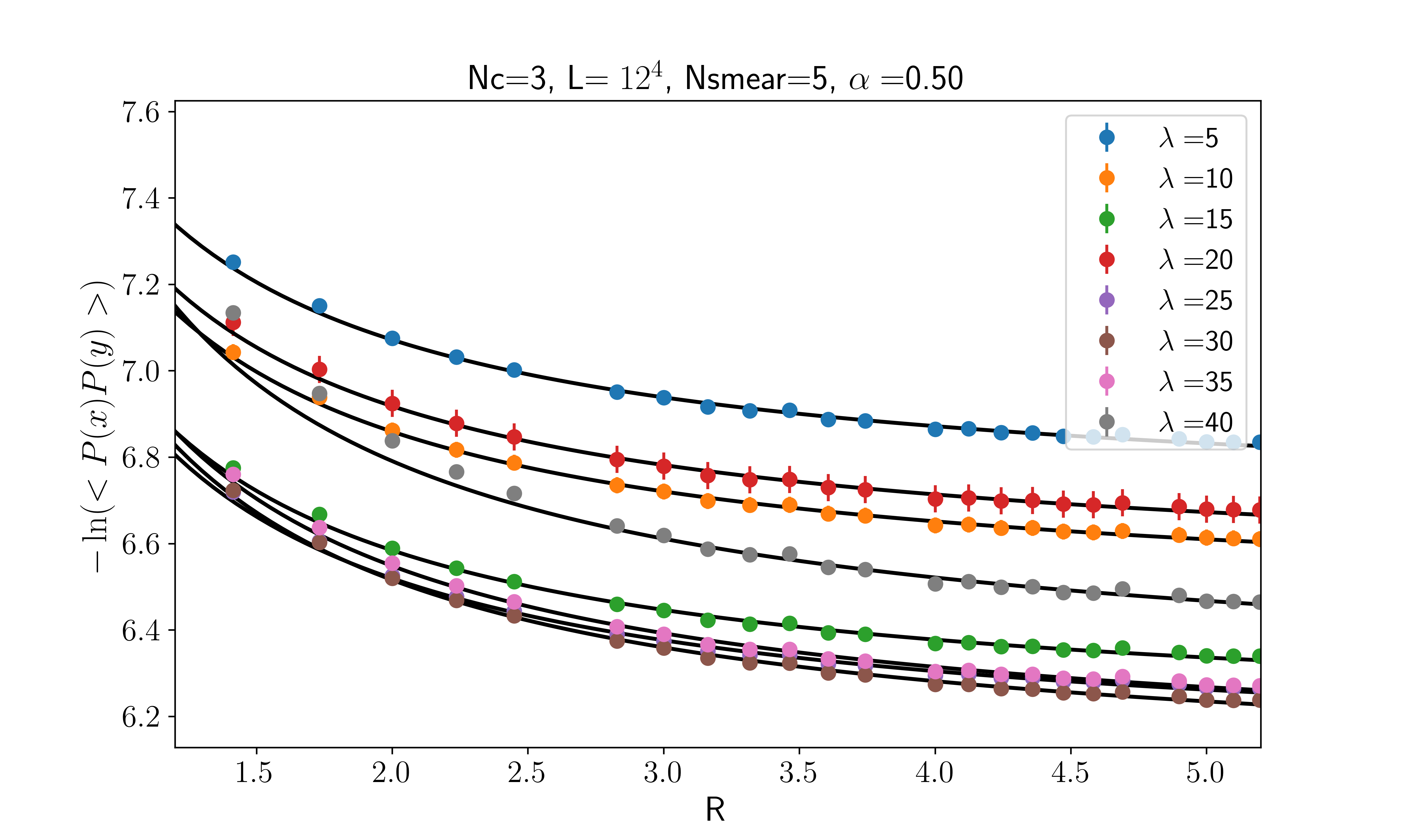
Figure 4: $-\ln{<P(x)P(y)>}$ vs $R$ for $12^{4}$ lattices at $\mu=0.05$ and $\kappa=1.0$

In practice we have computed this correlator on ensembles of smeared Polyakov lines. Smearing the lattice gauge fields is a procedure for replacing each of the lattice gauge links by an average over neighboring link paths or staples. This smearing procedure has the effect of reducing U.V effects and increasing the signal to noise ratio in observables that depend on the gauge field. It also suppresses the contribution of any bare quark mass. We have used the APE smearing procedure which replaces the link fields ${\cal U}$ in the following way

$${\cal U}_{a}(x)^{(N_{smear})}=(1-\alpha){\cal U}_{a}(x)^{(N_{smear}-1)}+\frac{\alpha}{8(1-\alpha)}{\cal S}_{a}(x)^{(N_{smear}-1)}$$ (18)

where ${\cal S}$ denotes the sum over directional staples, $N_{smear}$ denotes the number of iterative smearing steps and $\alpha$ is the smearing coefficient albanese1987glueball .

We have fitted the correlator for a range of smearing parameters at each value of $\lambda$ assuming a non-abelian Coulomb form for $V(r)$ – see the tables 1-3 in the appendix. In practice we find that $N_{smear}=5$ and $0.45\leq\alpha\leq 0.55$ yields good, robust fits to the data over the range $2<r<5$ on a $12^{4}$ lattice. Fig. 4 shows the logarithm of this correlator for a lattice of size $L=12^{4}$ with $\mu=0.05$ with $N_{smear}=5,\alpha=0.50$.

Taking the coefficients from these Coulomb fits and plotting them as a function of $\sqrt{\lambda}$ we again see a linear dependence on $\sqrt{\lambda}$ which is consistent with the holographic expectation Chu:2009qt . Indeed, even the numerical coefficient in the fit lies within $10\%$ or so of the holographic prediction which can be seen in fig.5. Note that the holographic prediction has been expressed in terms of the lattice coupling $\lambda$ and not the continuum coupling. In the appendix B we include equivalent fits (figs.10 and 10) for a range of different smearing parameters thereby verifying that the agreement with the holographic prediction is robust.

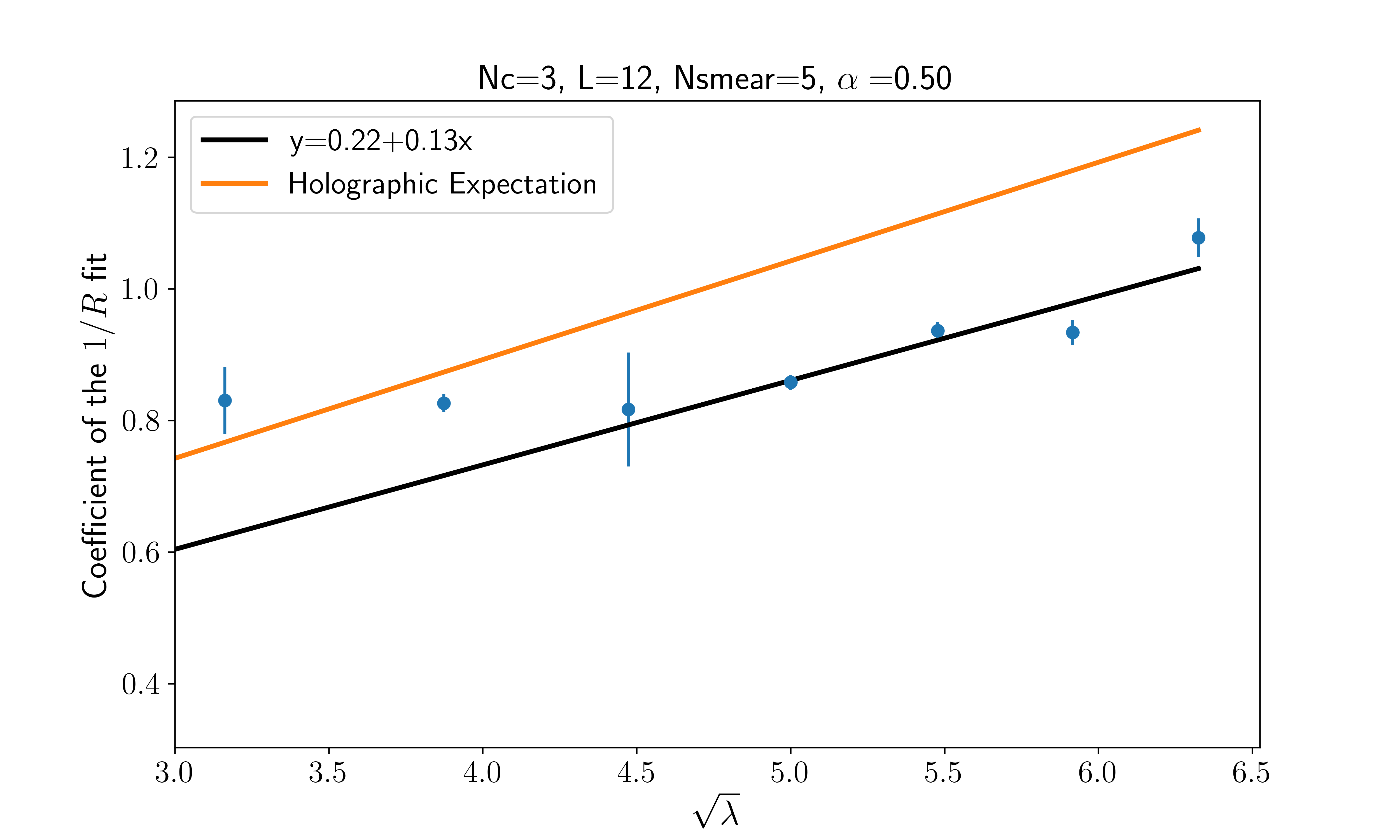
Figure 5: Coefficient of the $1/r$ vs $\sqrt{\lambda}$ for $12^{4}$ lattices at $\mu=0.05$

4 Conclusions

We have studied a new supersymmetric lattice action for ${\rm N}=4$ super Yang-Mills in four dimensions at strong ’t Hooft coupling. We have focused on the case of three colors $N=3$ and utilized lattices as large as $12^{4}$. Correlators of (smeared) Polyakov lines show that the static potential exhibits a non-Abelian Coulomb form $V(r)=\frac{\alpha\sqrt{\lambda}}{r}$ where the value of $\alpha$ and the square root dependence on the ’t Hooft coupling match expectations from holography.

Appendix A Appendix - Phase of the Pfaffian

Appendix B Appendix – Dependence of the fits on smearing parameters

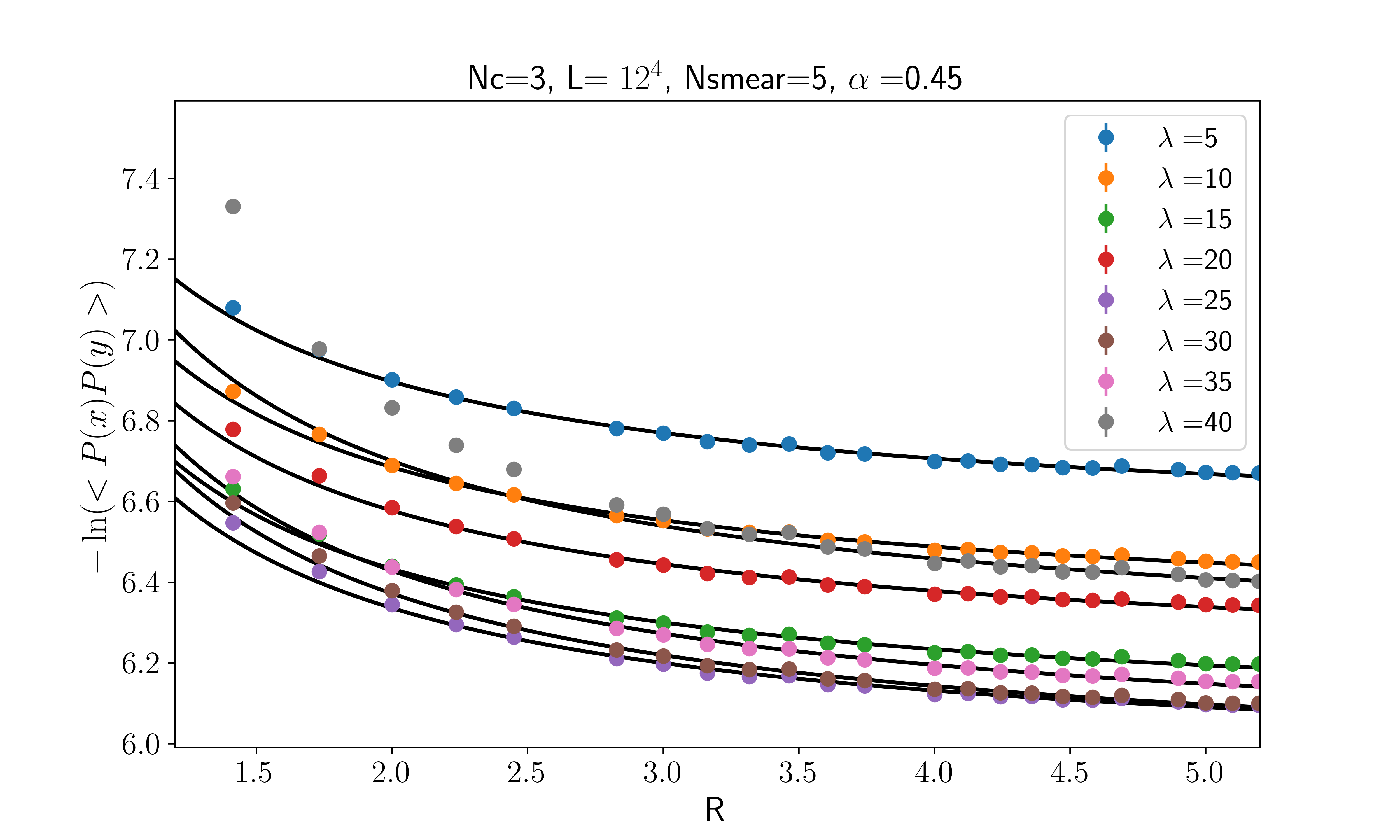
Figure 7: $-\ln{<P(x)P(y)>}$ for $\alpha=0.45$

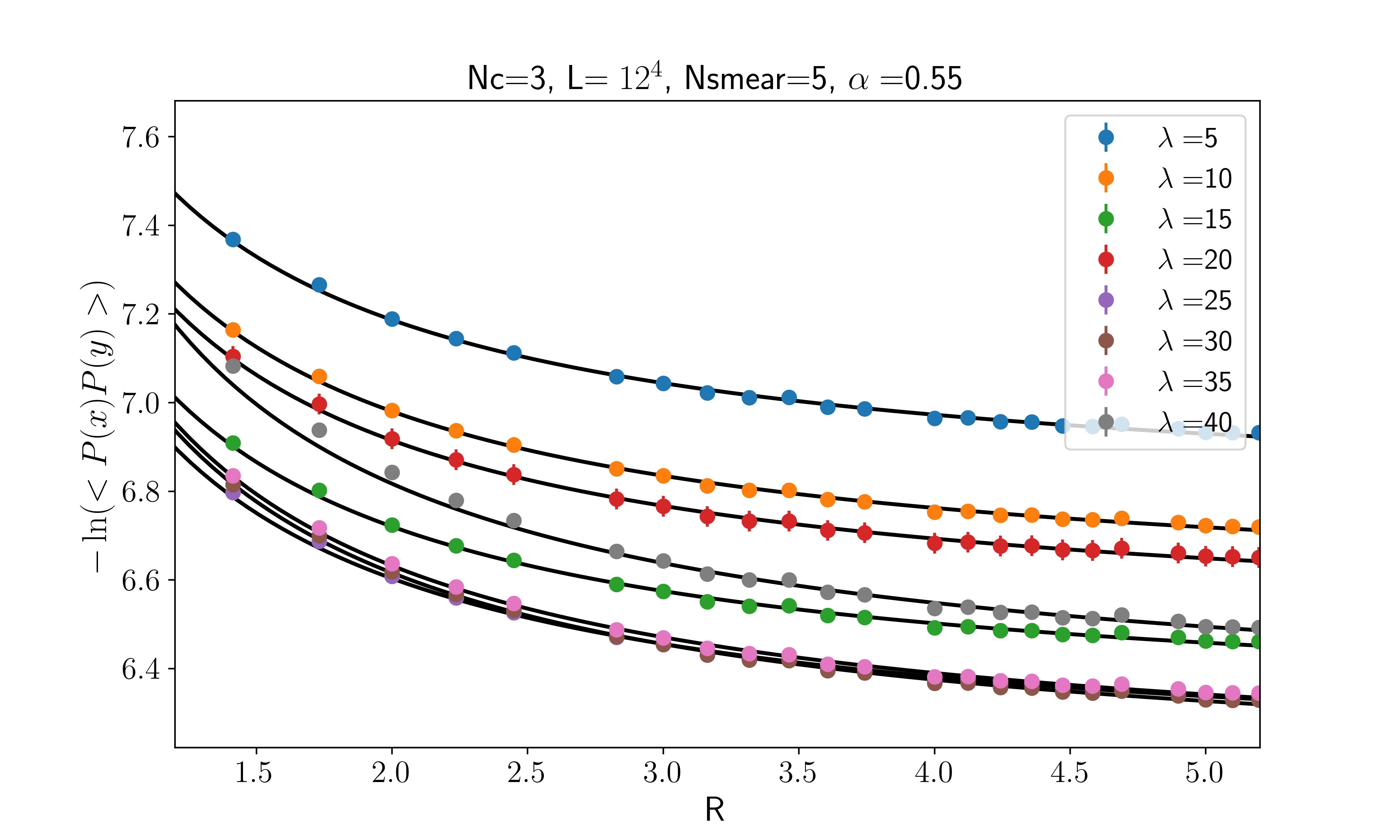
Figure 8: $-\ln{<P(x)P(y)>}$ for $\alpha=0.55$

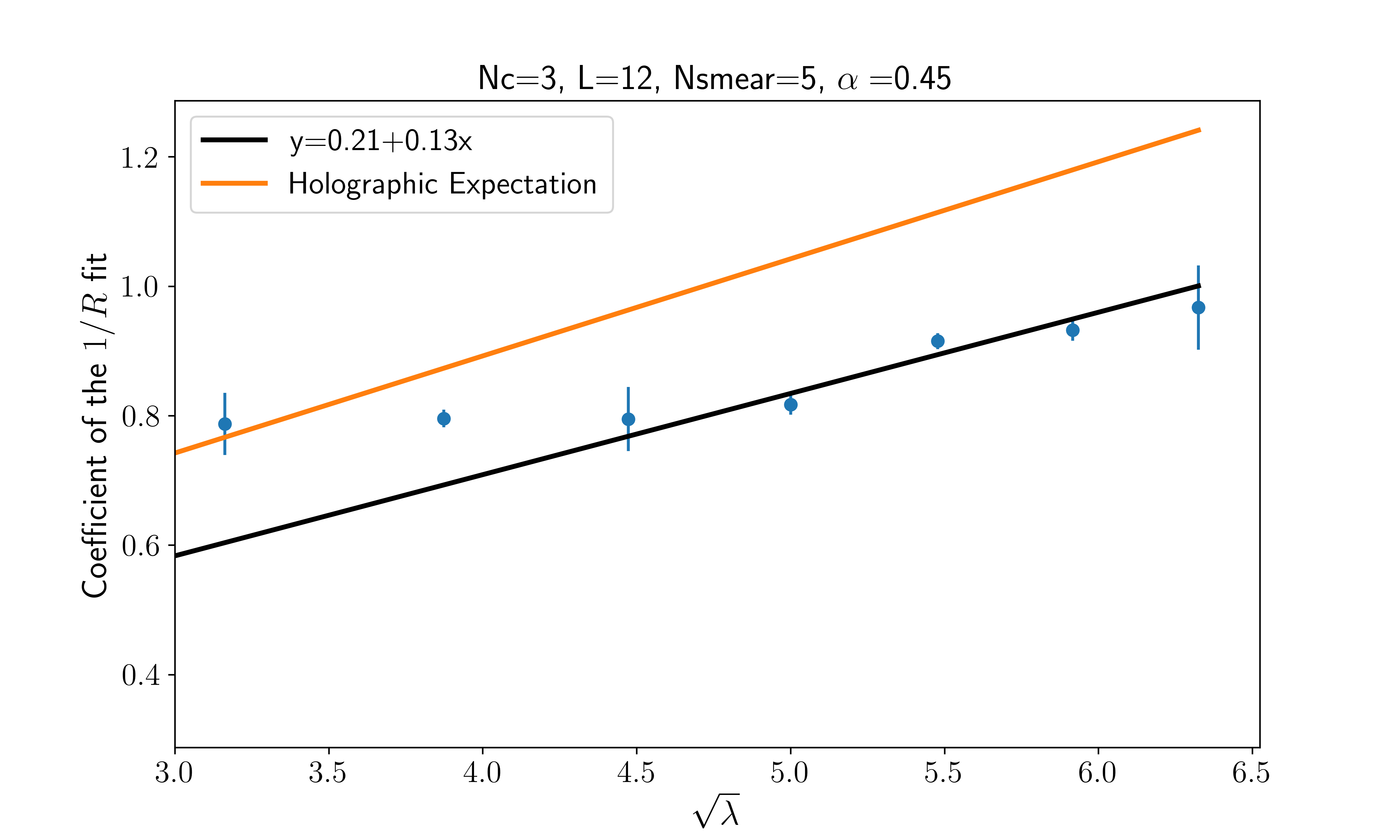
Figure 9: Coefficient of the $1/r$ vs $\sqrt{\lambda}$ for $\alpha=0.45$

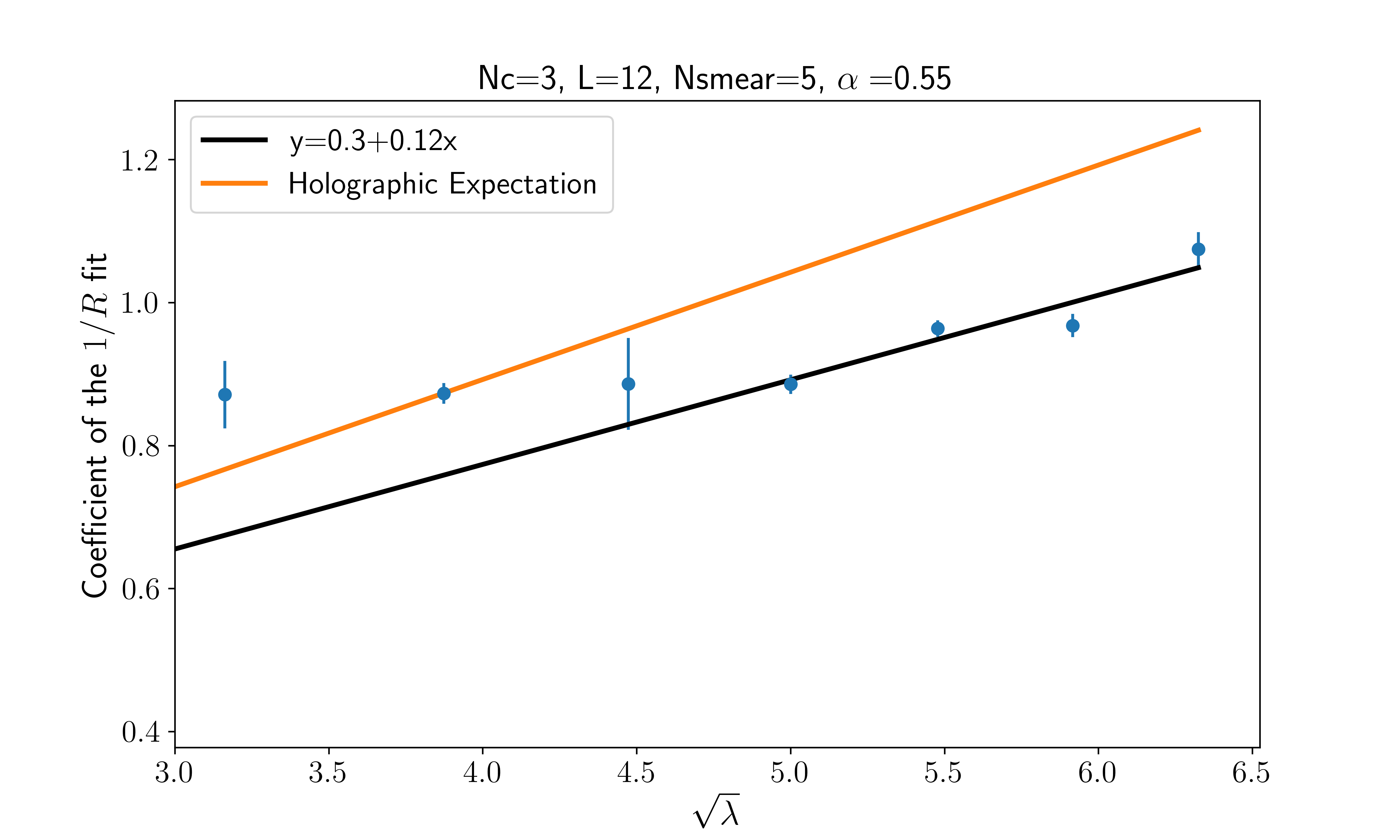
Figure 10: Coefficient of the $1/r$ vs $\sqrt{\lambda}$ for $\alpha=0.55$

$\lambda$	$a+b/R$	Reduced-$\chi^{2}$
$5$	$6.51(1)+0.76(3)/R$	0.18
$10$	$6.29(1)+0.78(5)/R$	0.085
$15$	$6.03(4)+0.79(1)/R$	1.6
$20$	$6.06(1)+0.80(5)/R$	0.13
$25$	$5.92(1)+0.81(2)/R$	1.4
$30$	$5.91(1)+0.92(1)/R$	1.8
$35$	$5.96(1)+0.93(2)/R$	1.2
$40$	$6.22(2)+0.97(1)/R$ ($3.5<R<5.0$)	2.3

Table 1: $1/R$ Fitting results for $L=12^{4},\mu=0.05,N_{smear}=5,\alpha=0.45$

$\lambda$	$a+b/R$	Reduced-$\chi^{2}$
$5$	$6.67(1)+0.79(4)/R$	0.16
$10$	$6.44(2)+0.83(5)/R$	0.07
$15$	$6.17(1)+0.82(1)/R$	1.50
$20$	$6.51(3)+0.81(8)/R$	0.04
$25$	$6.09(1)+0.86(2)/R$	2.10
$30$	$6.09(1)+0.937(1)/R$	1.34
$35$	$6.05(1)+0.934(2)/R$	0.92
$40$	$6.25(1)+1.07(2)/R$ ($3.0<R<5.0$)	3.03

Table 2: $1/R$ Fitting results for $L=12^{4},\mu=0.05,N_{smear}=5,\alpha=0.50$

$\lambda$	$a+b/R$	Reduced-$\chi^{2}$
$5$	$6.76(1)+0.85(3)/R$	0.17
$10$	$6.54(1)+0.87(5)/R$	0.09
$15$	$6.28(1)+0.87(1)/R$	1.23
$20$	$6.47(2)+0.88(6)/R$	0.06
$25$	$6.09(1)+0.88(1)/R$	1.53
$30$	$6.13(1)+0.96(1)/R$	1.47
$35$	$6.14(1)+0.97(2)/R$	0.90
$40$	$6.28(1)+1.07(2)/R$ ($2.5<R<5.0$)	2.48

Table 3: $1/R$ Fitting results for $L=12^{4},\mu=0.05,N_{smear}=5,\alpha=0.55$