Correspondence between field theory in Rindler frame and thermofield-double formalism

Abstract

Considering two accelerated observers with same acceleration in two timelike wedges of Rindler frame we calculate all the thermal Feynmann propagators for a real scalar field with respect to the Minkowski vacuum. Only the same wedge correlators are symmetric in exchange of thermal bath and Unruh thermal bath. Interestingly, they contains a cross term which is a collective effects of acceleration and thermal nature of field. Particularly the zero temperature description corresponds to usual thermofield double formalism. However, unlike in later formulation, the two fields are now parts of the original system. Moreover it bears the features of a spacial case of closed time formalism where the Keldysh contour is along the increasing Rindler time in the respective Rindler wedges through a specific complex time intra-connector. Hence Rindler frame field theory seems to be a viable candidate to deal thermal theory of fields and may illuminate the search for a bridge between the usual existing formalims.

1 Introduction

In zero-temperature limit the conventional quantum field theory (QFT) predictions match exceptionally well with the existing experiments. However, many real-world systems can not be well approximated as zero-temperature ones. The study of hot quark-gluon plasma [1, 2], thermal phase transitions [3, 2], cosmological inflation [4, 5, 6, 7, 8, 2], and the evolution of a neutron star [2] requires a sophisticated formalism of thermal field theory. There are various approaches to deal the thermal nature of a system. Usually the thermal ensemble average of any operator is done with the thermal density operator $\rho(\beta)=e^{-\beta\mathcal{H}}$ where $\beta$ and $\mathcal{H}$ are the inverse temperature and Hamiltonian of the system. A significant development in understanding the theory of fields in thermal equilibrium is made by Matsubara [9], which is known as Matsubara formalism or imaginary time formalism. In this formalism, time takes imaginary values from $0$ to $-i\beta$ and the limit variable $\beta$ plays the role of the system’s inverse temperature. The thermal Green function is then evaluated from that of the zero temperature field theory through an infinite series sum. The thermofield double (TFD) formalism [10, 11, 12] is another one in which thermal vacuum state is defined to mimic the ensemble average. In this construction, one needs to add a fictitious (tilde) system along with the original system, which is identical to the original system, except it follows conjugation rules [13, 10]. The TFD state (expressed as $|0,\beta\rangle$) is a superposition state of the combined eigenstates of two identical systems ($|n\rangle\otimes|\tilde{n}\rangle$) and is connected to the zero-temperature vacuum of the combined system by a Bogoliubov transformation. For this combined system, one may construct four types of the thermal propagators. These are, the Feynman propagator for the original system, the anti-Feynman propagator for the tilde system, and two cross propagators for combination of fields in both original and tilde systems. These propagators form a $2\times 2$ matrix comprising zero-temperature and thermal parts of the propagators. This formalism plays a vital role in understanding of the time-evolution of entanglement entropy [14, 15, 16, 17], scrambling and quantum chaos [18, 19, 20, 21], firewalls [22, 23, 24], ER=EPR [23, 25], and emergent spacetime [26], etc.

Close time path (CTP) formalism, also known as “in-in” or real-time formalism (mainly based on Schwinger-Keldysh formulation) is another one to deal thermal theory of fields [27, 28]. One particular choice of the Keldysh contour (see Fig. 1) has two real parts ($C_{+}$ and $C_{-}$) and two imaginary parts ($C_{3}$ and $C_{4}$). The assigning of two physical fields on two real time axes ($\phi_{+}$ on $C_{+}$ and $\phi_{-}$ on $C_{-}$) provides four components of propagator and therefore can be represented by a $2\times 2$ matrix. The branch $C_{2}$ has imaginary values from $0$ to $-i\sigma$ with $0\leq\sigma\leq\beta$. It has been observed that for the choice $\sigma=\beta/2$ provides the thermal propagators which are identical to those obtained in TFD with the identification original and tilde fields in TFD as $\phi=\phi_{+}$ and $\tilde{\phi}=\phi_{-}$, respectively. The time in the $C_{-}$ branch runs in the opposite direction as compared to the $C_{+}$ branch. This is analogous to the conjugation rule for the tilde fields in TFD. In spite of such similarities, these two formalims are not physically equivalent. In TFD the tilde field is fictitious and both the fields commute with each other. Whereas, the fields in CTP have physical existance and their commutation relations are not such trivial one. Moreover in interacting theory these formalisms behave differently.

Nonetheless, there are certain advantages in the respective formulations. As described, TFD is capable of describing the thermal-vacuum state, while CTP dose not. But the later one deals with two physically existing fields. Then naturally one might be wondering whether there is any other way of describing thermal field theory which can provide a middle root such that those issues can be tackled in a better way. We show here that the field theory in Rindler frame can be one such candidate. Let us now provide the motivation for such possibility. It is well known that an accelerated observer always gets casually restricted to a quadrant of the Minkowski spacetime. The null paths passing through the origin act as the Rindler horizons for the observer. These paths devide the whole spacetime into four parts: left (L), right (R), past (P), and future (F) Rindler wedges. In this case two timelike regions are possible, namely the right Rindler wedge (RRW) and the left Rindler wedge (LRW). The regions RRW and LRW are causally disconnected, and their coordinate times run in the opposite directions. Also existance of two fields ($\phi^{R}$ and $\phi^{L}$) natually appears in these two accelerating frames. These features are similar to CTP formalism. Moreover, since the respective frame see the Minkowski vacuum as thermal bath (known as Unruh effect [29, 30, 31, 32]), it is possible that the thermal vacuum state in TFD formalism can be mimicked by the Minkowski vacuum while expressing this as a linear combinations of composite Fock states of the two Rindler fields. Therefore it seems that the field theory in Rindler frames may be a natural candidate to describe thermal theory of fields.

In this paper we consider two observers which are accelerating with same constant acceleration $a$ in RRW and LRW, respectively. For generality, the Rindler fields (which are taken to be real scalar ones) are considered as thermal at inverse temperature $\beta_{0}$. All the possible combinations for Feynman progators, namely $G_{RR}$ , $G_{LL}$, $G_{RL}$ and $G_{LR}$, are being calculated through ensemble averaging procedure with respect to the vacuum of the Minkowski observer. We observe that $G_{RR}$ and $G_{LL}$ indivitually consists of four parts – usual non-thermal, thermal due to $\beta_{0}$, Unruh thermal due to acceleration at inverse temperature $\beta_{U}=2\pi/a$ and a cross term due to both $\beta_{0}$ as well as $\beta_{U}$. These two correlators are symmetric under the exchange of $\beta_{0}\leftrightarrow\beta_{U}$. Whereas other two consist of a pure Unruh thermal and a cross-term. These do not carry the symmetric property. The cross contribution is usually interpreted as the stimulating effect due to presence of both actual thermal and Unruh thermal baths [33, 34]. This structure of Feynman propagators implies that in presence of interaction the physical quantities in Rindler frame will not only be affected by acceleration which is exactly like the same due to $\beta_{0}$, but also a stimulating effect must show its presence.

Among the two limits, $\beta_{U}\to\infty$ and $\beta_{0}\to\infty$, we observe that the later one is very interesting. For this the Rindler propagators reduce to those in TFD with the identifications $\phi^{R}\equiv\phi$, $\phi^{L}\equiv\tilde{\phi}$ and $\beta_{U}\equiv\beta$. Thus must be identical to those in CTP for $\sigma=\beta_{U}/2$. Thus our investigation suggests a profound correspondence between the accelerated and thermal systems. Such an observation has various implications. These are as follows.

• Unlike TFD, in the two Rindler wedges we have two physical fields and therefore these are parts of our system. Moreover the thermal vacuum can be constructed from composite Fock space of these fields. Therefore such an analysis not only encodes the logistics of TFD, but also provides more physical picture in terms of the realization of both the fields.

• Similar to CTP, in our discussion we have a clear Keldysh contour for the Rindler time coordinate $\eta$. One part is the hyperbolic path in RRW, runs from $\eta=-\infty$ to $\eta=\infty$. The last part is the hyperbolic trajectory in LRW (runs from $\eta=\infty$ to $\eta=-\infty$) which is the mirror image of that in RRW. They are connected by a complex branch from $\eta=\infty$ to $\eta=\infty-i\beta_{U}/2$. Therefore Rindler frame QFT also encodes the language of CTP. But here, unlike CTP, both the fields commute with each other.

In summary, the zero temperature ($\beta_{0}\to\infty$) field theory in Rindler frames, at least in the non-interacting level, can completely mimic the TFD formalism with added avantages like both the fields are now parts of the original system and can also encode features of CTP. Therefore we feel that this can be a deserving formalism to deal thermal theory of fields and also can be possible candidate to bridge between CTP and TFD for $\sigma=\beta/2=\beta_{U}/2$.

We organize this paper in the following way. In Sec. 2, a brief review on TFD and CTP is presented. Sec. 3 contains the main results regarding the thermal propagators in Rindler frame with respect to Minkowski vacuum. In this section we discuss the implications of our investigation and possible relation with TFD and CTP. Finally, in Sec. 4, we conclude.

2 Brief review of the Thermofield dynamics

The ensemble average value of an observable $A$ for a system (denoted by Hamiltonian $H=\sum_{\textbf{k}}\omega_{\textbf{k}}a_{\textbf{k}}^{\dagger}a_{\textbf{k}}$) in thermal equilibrium at inverse temperature $\beta$ is given by $\langle A\rangle_{\beta}={\text{Tr}(e^{-\beta H}A)}/{\text{Tr}(e^{-\beta H})}$. In this formulation the thermal Green’s function in field theory can be expressed as the sum of a infinite series for the Green’s function corresponding to zero temperature field theory with the complexification of time. This is known as Matsubara [9] or the imaginary time formalism. On the other hand such an averaging process can be equivalently described by introducing a thermal vacuum state ($|0,\beta\rangle$) such that $\langle 0,\beta|A|0,\beta\rangle=\langle A\rangle_{\beta}$. In order to construct the state, one introduces a fictitious system, which is identical to the original system, except it follows a tilde conjugation rule [10, 35]. This is known as thermofield double state (TFD) formalism. For the scalar field, this is given by [10]

$$|0,\beta\rangle=U(\theta)|0,\tilde{0}\rangle=e^{-\sum_{\textbf{k}}\theta_{\textbf{k}}(\beta)(\tilde{a}_{\textbf{k}}a_{\textbf{k}}-a_{\textbf{k}}^{\dagger}\tilde{a}_{\textbf{k}}^{\dagger})}|0,\tilde{0}\rangle\,=\frac{1}{\sqrt{Z(\beta)}}\sum_{\textbf{k},n_{\textbf{k}}}e^{-\beta n_{\textbf{k}}\omega_{\textbf{k}}/2}|n_{\textbf{k}},\,\tilde{n}_{\textbf{k}}\rangle\,~{},$$ (1)

where $Z(\beta)=\sum_{\textbf{k}}(1-e^{-\beta\omega_{\textbf{k}}})^{-1}$. In the above tilde denotes quantities for fictitious system whereas without tilde ones are for original system. $|n_{\textbf{k}},\,\tilde{n}_{\textbf{k}}\rangle\,$ is the Fock space for the composite system. The variable $\theta$ is function of $\beta$, and is given by $\tanh\theta_{\textbf{k}}(\beta)=e^{-\beta\omega_{\textbf{k}}/2}$.

In this formalism the thermal propagator is defined through $iG_{\beta}(x,y)=\langle 0,\beta|\mathcal{T}[\Phi(x)\Phi^{T}(y)]|0,\beta\rangle$ where

$$\Phi(x)=\begin{pmatrix}\phi(x)\\ \tilde{\phi}(x)\end{pmatrix}$$ (2)

is a doublet constructed by original field $\phi(x)$ and tilde field $\tilde{\phi}(x)$ configurations. $\mathcal{T}$ and $T$ denote time-ordering and transpose, respectively. The propagator is represented by a $2\times 2$ matrix. In momentum space this is given by

$$G_{\beta}(k) =\begin{pmatrix}\frac{1}{k^{2}-m^{2}+i\epsilon}&0\\ 0&-\frac{1}{k^{2}-m^{2}-i\epsilon}\end{pmatrix}-2i\pi\,n_{\beta}(|k^{0}|)\,\delta(k^{2}-m^{2})\begin{pmatrix}1&e^{\beta|k^{0}|/2}\\ e^{\beta|k^{0}|/2}&1\end{pmatrix}\,,$$ (3)

where $n_{\beta}(|k^{0}|)=(e^{\beta\omega_{\textbf{k}}}-1)^{-1}$ is bosonic number density. Here $k^{2}$ is the square of norm of the four-momentum, $m$ is the mass of the field and $|k^{0}|=\omega_{\textbf{k}}=(\textbf{k}^{2}+m^{2})^{1/2}$. The first and last diagonal elements are Feynman propagators for $\phi$ and $\tilde{\phi}$, respectively. The off-diagonals terms are ($\langle\phi\tilde{\phi}\rangle$ (top-right term) and$\langle\tilde{\phi}\phi\rangle$ (bottom-left term)) cross propagators between the original and the tilde fields. The thermal propagator has two contributions: the non-thermal propagator and the temperature dependent contributions. The thermal contribution contains bosonic number density and a Dirac delta function selecting only the on-shell modes. Due to the thermal contributions the off-diagonal terms are also non-vanishing.

Another approach to thermal field theory which is reminiscent to TFD is the closed time path (CTP) formalism. Such a formalism is based on a particular choice of Keldysh contour. For the choice, as shown in Fig. 1

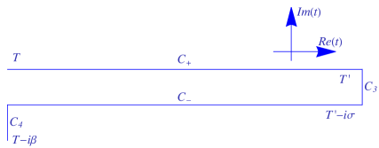
Figure 1: Closed time contour of Schwinger-Keldysh formalism with real branches $C_{+}$ and $C_{-}$, imaginary branches $C_{3}$ and $C_{4}$. Here one take the limits $T\to-\infty$ and $T^{\prime}\to\infty$. For thermal system we have $\sigma=\beta/2$.

one introduces two-field configurations. The parts of the contour can be named as $C_{+}$, $C_{-}$ $C_{3}$ and $C_{4}$. On $C_{+}$ and $C_{-}$ branches time runs from $-\infty$ to $\infty$ and from $\infty$ to $-\infty$, respectively. In the imaginary time branches $C_{3}$ and $C_{4}$ time ranges are $(\infty$,$\infty-i\sigma$) and ($-\infty-i\sigma$, $-\infty-i\beta$), respectively with $0\leq\sigma\leq\beta$. We denote the field lying on $C_{+}$ branch as $\phi_{+}$ and the same on $C_{-}$ is labeled as $\phi_{-}$. In this formalism the propagator is represented by $2\times 2$ matrix as well and is given by

$$G(k)=\begin{pmatrix}G_{++}&G_{+-}\\ G_{-+}&G_{--}\end{pmatrix}=\begin{pmatrix}\frac{1}{k^{2}-m^{2}+i\epsilon}&0\\ 0&-\frac{1}{k^{2}-m^{2}-i\epsilon}\end{pmatrix}$$

$$-2i\pi\,\delta(k^{2}-m^{2})\begin{pmatrix}n_{\beta}(\omega_{\textbf{k}})\,&e^{\sigma\omega_{\textbf{k}}}(n_{\beta}(\omega_{\textbf{k}})\,+\Theta(-\omega_{\textbf{k}}))\\ e^{-\sigma\omega_{\textbf{k}}}(n_{\beta}(\omega_{\textbf{k}})\,+\Theta(\omega_{\textbf{k}}))&n_{\beta}(\omega_{\textbf{k}})\,\end{pmatrix}\,.$$ (4)

Here, $\Theta$ is the Heaviside step function. The first-row elements are for $(t,t^{\prime}\in C_{+})$ and $(t,\in C_{+};\,t^{\prime}\in C_{-})$, respectively. While those in the second row are for $(t,\in C_{-};\,t^{\prime}\in C_{+})$ and $(t,t^{\prime}\in C_{-})$, respectively.

Although (2) are (3)) in-general different, but for a specific choice $\sigma=\beta/2$ they coincide. In this particular case it appears that $\phi=\phi_{+}$ and $\tilde{\phi}$ gets a physical identity as $\phi_{-}$ and hence TFD and CTP are equivalent formalisms. But in reality these are not physically equivalent. In TFD different fields commute whereas the commutation relation between two types of fields in CTP is different. Also in presence of interactions, these two formalisms behave differently.

So far we observed that TFD and CTP formalisms, although physically different, conicide at free theory level for a certain choice of $\sigma$. Moreover there are certain advantages or disadvantages in the respective formulations. For example, TFD is capable of describing the thermal-vacuum state; but deals with a fictitious field. Whereas as CTP dose suffer from the first issue while it is free of later one. Then naturally one might be wondering whether there is any other way of describing thermal field theory which can provide a middle root such that those issues can be tackled in a better way. We found that field theory in Rindler frame can be one such candidate. Let us now provide the motivation for such possibility and show how far we can proceed.

3 Free field theory in Rindler frame

In $(1+1)$-dimension trajectory of a uniformly accelerated observer with uniform acceleration $a$ is given by the coordinate transform

$$t=\frac{e^{a\xi}}{a}\sinh{a\eta};~{}~{}x=\frac{e^{a\xi}}{a}\cosh{a\eta}\,,$$ (5)

where $(t,x)$ are the Minkowski coordinates. And $(\eta,\,\xi)$ are the Rindler coordinates, which are extended from $-\infty$ to $\infty$. However these coordinate system covers only a single quadrant (where $|t|<x$) of the total Minkowski spacetime. This region is called the right Rindler wedge (RRW). In a similar way one may get another Rindler wedge by the following transformation

$$t=-\frac{e^{a\xi^{\prime}}}{a}\sinh{a\eta^{\prime}};~{}~{}x=-\frac{e^{a\xi^{\prime}}}{a}\cosh{a\eta^{\prime}}\,,$$ (6)

where the coordinates covers the region bounded by $|t|<-x$. This region is known as the left Rindler wedge. There are another two Rindler wedges, known as the future and past Rindler wedges (FRW and PRW). Since timelike trajectories can be formed only in RRW and LRW, it is then natural to consider two obserevers which can be thought of two systems. Under these frames one can the introduce two species of fields. Therefore such two accelerated frames can describe two physically existing fields – one is lying in RRW and another is in LRW.

The trajectories of an accelerated observers are provided by a hyperbola as shown in Fig. 2. Coordinate transformation of the both regions give the same line element as

$$ds^{2}=e^{2a\xi}\left[d\eta^{2}-d\xi^{2}\right]\,,$$ (7)

which is conformally flat and one obtain the KG modes in the right and left Rindler wedges as [31, 36]

$${}^{R}u_{k} =\frac{1}{\sqrt{4\pi\omega_{\textbf{k}}}}e^{i\textbf{k}\xi-i\omega_{\textbf{k}}\eta}~{}~{}~{}\textup{in~{}RRW}$$ (8)

$$=0~{}~{}~{}~{}~{}~{}~{}~{}~{}~{}~{}~{}~{}~{}~{}~{}~{}~{}~{}~{}\textup{in~{}LRW}$$

$${}^{L}u_{k} =\frac{1}{\sqrt{4\pi\omega_{\textbf{k}}}}e^{i\textbf{k}\xi+i\omega_{\textbf{k}}\eta}~{}~{}~{}\textup{in~{}LRW}$$

$$=0~{}~{}~{}~{}~{}~{}~{}~{}~{}~{}~{}~{}~{}~{}~{}~{}~{}~{}~{}~{}\textup{in~{}RRW}.$$

These sets of modes are complete in either RRW or LRW, not in the full Minkowski space. However they together are forms complete basis for the whole spacetime. Using them one can find two physical entities of field configuration corresponding to two Rindler observers:

$$\phi^{R}(x) =\sum_{\textbf{k}=-\infty}^{\infty}\left[b^{R}_{\textbf{k}}~{}^{R}u_{\textbf{k}}+b^{R^{\dagger}}_{\textbf{k}}~{}^{R}u_{\textbf{k}}^{*}\right]\,,$$ (9)

$$\phi^{L}(x) =\sum_{\textbf{k}=-\infty}^{\infty}\left[b^{L}_{\textbf{k}}~{}^{L}u_{\textbf{k}}+b^{L^{\dagger}}_{\textbf{k}}~{}^{L}u_{\textbf{k}}^{*}\right]\,.$$

Superscript $L$ and $R$ correspond to the left and the right Rindler wedges respectively, and the annihilation operators $b_{\textbf{k}}^{R,L}$ annihilate the Rindler vacuum $|0_{\mathcal{R}}\rangle$. To make life easy it will be better to work with Unruh operators $(d^{1}_{k},d^{2}_{k})$ which annihilate the Minkowski Vacuum $(d^{1}_{\textbf{k}}|0_{M}\rangle=d^{2}_{\textbf{k}}|0_{M}\rangle=0)$, provided by Unruh [29] in $1976$. Then the above becomes [31]

$$\phi^{R}(x) =\sum_{\textbf{k}=-\infty}^{\infty}\frac{1}{\sqrt{2\sinh{\frac{\pi\omega_{\textbf{k}}}{a}}}}\left[d^{1}_{\textbf{k}}~{}e^{\frac{\pi\omega}{2a}}~{}^{R}u_{\textbf{k}}+d^{2}_{\textbf{k}}~{}e^{-\frac{\pi\omega}{2a}}~{}^{R}u^{*}_{-\textbf{k}}\right]+h.c.\,,$$

$$\phi^{L}(x) =\sum_{\textbf{k}=-\infty}^{\infty}\frac{1}{\sqrt{2\sinh{\frac{\pi\omega_{\textbf{k}}}{a}}}}\left[d^{1}_{\textbf{k}}e^{-\frac{\pi\omega_{\textbf{k}}}{2a}}~{}^{L}u^{*}_{-\textbf{k}}+d^{2}_{\textbf{k}}e^{\frac{\pi\omega_{\textbf{k}}}{2a}}~{}^{L}u_{\textbf{k}}\right]+h.c.\,.$$

In this discussion for generality we consider the fields are inherently thermal with same inverse temperature $\beta_{0}$. Then defining the Wightman function with respect to Minkowski vacuum as $G_{W_{ij}}(x_{1},x_{2})=\langle 0_{M}|e^{-\beta_{0}(H_{i}+H_{j})}\phi^{i}(\eta_{1},\xi_{1})\phi^{j}(\eta_{2},\xi_{2})|0_{M}\rangle/Z(\beta_{0})$ under the concept of ensemble average of the field operators, we have four propagators. We name the propagators as $G_{W_{RR}},\,G_{W_{RL}},\,,G_{W_{LR}}$ and $G_{W_{LL}}$. We also consider equal magnitudes of the acceleration for both observers. We obtain the following Wightman functions [37]

$$G_{W_{RR}}\left(\Delta\xi,\Delta\eta\right)= \int_{-\infty}^{\infty}\frac{d\textbf{k}~{}n_{\beta_{0}}(\omega_{\textbf{k}})}{8\pi\omega_{\textbf{k}}\sinh{\frac{\pi\omega_{\textbf{k}}}{a}}}\left[e^{\beta_{0}\omega_{\textbf{k}}}(\omega)\left\{e^{i\textbf{k}\Delta\xi-i\omega_{\textbf{k}}\Delta\eta}~{}e^{\frac{\pi\omega_{\textbf{k}}}{a}}+e^{i\textbf{k}\Delta\xi+i\omega_{\textbf{k}}\Delta\eta}~{}e^{-\frac{\pi\omega_{\textbf{k}}}{a}}\right\}\right.$$ (10)

$$\left.~{}~{}~{}~{}~{}~{}~{}~{}~{}~{}~{}~{}~{}~{}~{}~{}~{}~{}~{}~{}~{}~{}~{}+\left\{e^{-i\textbf{k}\Delta\xi+i\omega_{\textbf{k}}\Delta\eta}~{}e^{\frac{\pi\omega_{\textbf{k}}}{a}}+~{}e^{-i\textbf{k}\Delta\xi-i\omega_{\textbf{k}}\Delta\eta}~{}e^{-\frac{\pi\omega_{\textbf{k}}}{a}}\right\}\right]\,;$$

$$G_{W_{LL}}\left(\Delta\xi,\Delta\eta\right)= \int_{-\infty}^{\infty}\frac{d\textbf{k}~{}n_{\beta_{0}}(\omega_{\textbf{k}})}{8\pi\omega_{\textbf{k}}\sinh{\frac{\pi\omega_{\textbf{k}}}{a}}}\left[e^{\beta_{0}\omega_{\textbf{k}}}\left\{e^{i\textbf{k}\Delta\xi+i\omega_{\textbf{k}}\Delta\eta}~{}e^{\frac{\pi\omega_{\textbf{k}}}{a}}+e^{i\textbf{k}\Delta\xi-i\omega_{\textbf{k}}\Delta\eta}~{}e^{-\frac{\pi\omega_{\textbf{k}}}{a}}\right\}\right.$$

$$\left.~{}~{}~{}~{}~{}~{}~{}~{}~{}~{}~{}~{}~{}~{}~{}~{}~{}~{}~{}~{}~{}~{}~{}+\left\{e^{-i\textbf{k}\Delta\xi-i\omega_{\textbf{k}}\Delta\eta}~{}e^{\frac{\pi\omega_{\textbf{k}}}{a}}+~{}e^{-i\textbf{k}\Delta\xi+i\omega_{\textbf{k}}\Delta\eta}~{}e^{-\frac{\pi\omega_{\textbf{k}}}{a}}\right\}\right]\,;$$

$$G_{W_{LR}}\left(\Delta\xi,\Delta\eta\right)= \int_{-\infty}^{\infty}\frac{d\textbf{k}~{}n_{\beta_{0}}(\omega_{\textbf{k}})}{8\pi\omega_{\textbf{k}}\sinh{\frac{\pi\omega_{\textbf{k}}}{a}}}\left[e^{\beta_{0}\omega_{\textbf{k}}}\left\{e^{i\textbf{k}\Delta\xi-i\omega_{\textbf{k}}\Delta\eta}+e^{i\textbf{k}\Delta\xi+i\omega_{\textbf{k}}\Delta\eta}\right\}\right.$$

$$\left.~{}~{}~{}~{}~{}~{}~{}~{}~{}~{}~{}~{}~{}~{}~{}~{}~{}~{}~{}~{}~{}~{}~{}+\left\{e^{-i\textbf{k}\Delta\xi+i\omega_{\textbf{k}}\Delta\eta}+~{}e^{-i\textbf{k}\Delta\xi-i\omega_{\textbf{k}}\Delta\eta}~{}\right\}\right]\,;$$

$$G_{W_{RL}}\left(\Delta\xi,\Delta\eta\right)= \int_{-\infty}^{\infty}\frac{d\textbf{k}~{}n_{\beta_{0}}(\omega_{\textbf{k}})}{8\pi\omega_{\textbf{k}}\sinh{\frac{\pi\omega_{\textbf{k}}}{a}}}\left[e^{\beta_{0}\omega_{\textbf{k}}}\left\{e^{-i\textbf{k}\Delta\xi+i\omega_{\textbf{k}}\Delta\eta}+e^{-i\textbf{k}\Delta\xi-i\omega_{\textbf{k}}\Delta\eta}\right\}\right.$$

$$\left.~{}~{}~{}~{}~{}~{}~{}~{}~{}~{}~{}~{}~{}~{}~{}~{}~{}~{}~{}~{}~{}~{}~{}+\left\{e^{i\textbf{k}\Delta\xi-i\omega_{\textbf{k}}\Delta\eta}+~{}e^{i\textbf{k}\Delta\xi+i\omega_{\textbf{k}}\Delta\eta}~{}\right\}\right]\,.$$

Having these positive frequency Wightman functions, we can now define the respective Feynman-like propagators through the relation

$$iG_{{ij}}\left(\Delta\xi,\Delta\eta\right)= \theta(\Delta\eta)G_{W_{ij}}\left(\Delta\xi,\Delta\eta\right)+\theta(-\Delta\eta)G_{W_{ij}}\left(\Delta\xi,-\Delta\eta\right)\,,$$ (11)

where the subscripts are $i,\,j=R,\,L$. In $4$-momentum space these are given by

$$iG_{{RR}}({k}) =\int_{-\infty}^{\infty}d\Delta\eta\int_{-\infty}^{\infty}d\Delta\xi\,iG_{{RR}}\left(\Delta\xi,\Delta\eta\right)\,e^{-i{\textbf{k}}\Delta\xi+i{\omega}\Delta\eta}$$ (12)

$$=i\,\left\{\frac{1}{({\omega}^{2}-\omega_{{\textbf{k}}}^{2}+i\epsilon)}-2i\pi\,n_{\beta_{0}}\,\delta({\omega}^{2}-\omega_{{\textbf{k}}}^{2})-2i\pi\,n_{a}\,\delta({\omega}^{2}-\omega_{{\textbf{k}}}^{2})-4i\pi\,n_{\beta_{0}}\,n_{a}\,\delta({\omega}^{2}-\omega_{{\textbf{k}}}^{2})\right\}$$

$$=i\,\left\{\frac{1}{({k}^{2}-m^{2}+i\epsilon)}-2i\pi\,n_{\beta_{0}}\,\delta({k}^{2}-m^{2})-2i\pi\,n_{a}\,\delta({k}^{2}-m^{2})-4i\pi\,n_{\beta_{0}}\,n_{a}\,\delta({k}^{2}-m^{2})\right\}\,,$$

$$iG_{{LL}}({k}) =\int_{-\infty}^{\infty}d\Delta\eta\int_{-\infty}^{\infty}d\Delta\xi\,iG_{{LL}}\left(\Delta\xi,\Delta\eta\right)\,e^{-i{\textbf{k}}\Delta\xi+i{\omega}\Delta\eta}$$ (13)

$$=i\,\left\{-\frac{1}{({\omega}^{2}-\omega_{{\textbf{k}}}^{2}-i\epsilon)}-2i\pi\,n_{\beta_{0}}\,\delta({\omega}^{2}-\omega_{{\textbf{k}}}^{2})-2i\pi\,n_{a}\,\delta({\omega}^{2}-\omega_{{\textbf{k}}}^{2})-4i\pi\,n_{\beta_{0}}\,n_{a}\,\delta({\omega}^{2}-\omega_{{\textbf{k}}}^{2})\right\}$$

$$=i\,\left\{-\frac{1}{({k}^{2}-m^{2}-i\epsilon)}-2i\pi\,n_{\beta_{0}}\,\delta({k}^{2}-m^{2})-2i\pi\,n_{a}\,\delta({k}^{2}-m^{2})-4i\pi\,n_{\beta_{0}}\,n_{a}\,\delta({k}^{2}-m^{2})\right\}\,.$$

$$iG_{{RL}}({k}) =\int_{-\infty}^{\infty}d\Delta\eta\int_{-\infty}^{\infty}d\Delta\xi\,iG_{{RL}}\left(\Delta\xi,\Delta\eta\right)\,e^{-i{\textbf{k}}\Delta\xi+i{\omega}\Delta\eta}$$ (14)

$$=i\,e^{\frac{\pi\omega_{{\textbf{k}}}}{a}}\,n_{a}\,\left(2\,n_{\beta_{0}}+1\right)\left[-2i\pi\delta({\omega}^{2}-\omega_{{\textbf{k}}}^{2})\right]$$

$$=i\,e^{\frac{\pi\omega_{{\textbf{k}}}}{a}}\,n_{a}\,\left(2\,n_{\beta_{0}}+1\right)\left[-2i\pi\delta({k}^{2}-m^{2})\right]\,=iG_{{LR}}({k}).$$

In the above we define ${k}=({\omega},\,{\textbf{k}})$, $\omega_{{\textbf{k}}}^{2}={\textbf{k}}^{2}+m^{2}$, $n_{\beta_{0}}=(e^{\beta_{0}\omega_{\bf{k}}}-1)^{-1}$ and $n_{a}=(e^{\frac{2\pi\omega_{\bf{k}}}{a}}-1)^{-1}$. Explicite steps to obtain the above forms are given in Supplemental meaterial. Here both $iG_{{RR}}({k})$ and $iG_{{LL}}({k})$ have four terms. The first term is independent of temperature and acceleration of the detectors. This represents the propagator for inertial motion of the observers in the zero-temperature field theory. The second term has only temperature dependent. The first and second terms together represent the propagator for inertial observers in finite temperature. The third term has only acceleration dependent, shows the contribution for accelerated motion of the detectors in the zero-temperate field theory. However the last term contains both temperature and motion dependence. Moreover, these are symmetric under the exchange of $\beta_{0}\leftrightarrow\beta_{U}=2\pi/a$, where $\beta_{U}$ is the inverse Unruh temperature. This is the reflection of the well known fact that the field theory in indivitual Rindler frame mimics thermal field theory. On the other hand other two are not in similar structure. Presence of cross terms in the propagators implies that the calculation of the physical quantities in interaction scenario with respect to Rindler frame not only contributed by acceleration effect which is identical to thermal field theory in Minkowski frame, but also by a stimulating effect in which $\beta_{0}$ and $\beta_{U}$ are stimulating each other. Let us now consider two important limits – one is $\beta_{0}\to\infty$ and other one is $\beta_{U}\to\infty$.

For the first limit (corresponds to zero temperature field theory in Rindler frame) the above reduces to

$$G_{{RR}}({k})=\frac{1}{({k}^{2}-m^{2}+i\epsilon)}-2i\pi\,n_{a}\,\delta({k}^{2}-m^{2})\,,$$ (15)

$$G_{{LL}}({k})=-\frac{1}{({k}^{2}-m^{2}-i\epsilon)}-2i\pi\,n_{a}\,\delta({k}^{2}-m^{2})\,,$$ (16)

$$G_{{RL}}({k})=e^{\frac{\pi\omega_{{\textbf{k}}}}{a}}\,n_{a}\,\left[-2i\pi\delta({k}^{2}-m^{2})\right]\,=G_{{LR}}({k})\,.$$ (17)

Arranging these in the following matrix form:

$$G=\begin{pmatrix}G_{RR}&G_{RL}\\ G_{LR}&G_{LL}\end{pmatrix}\,.$$ (18)

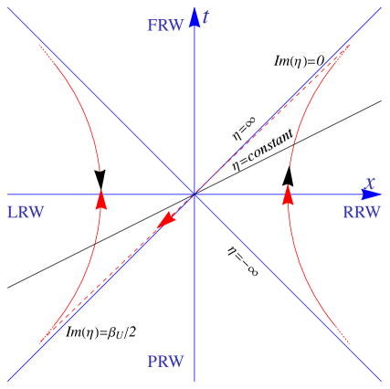
Figure 2: Trajectory of an accelerated detector in RRW and LRW are shown as red hyperbolas. The black arrows represent direction of the Rindler time propagation. The Rindler time ($\eta$) in RRW is increasing upward. In LRW, it is decreasing upward. The dashed red line represents a complex Rindler time propagation (consider it as an imaginary line in complex $\eta$-plane), connecting two Rindler time branches in RRW and LRW. The red arrows represent the direction of time ($\eta$) propagation in the closed contour.

we observe that this is identical to that of TFD (see Eq. (3)) with the identification $\beta_{U}=\beta$. Thus the propagators of two accelerated observers in right and left Rindler wedges in zero-temperature field theory have same structure as the thermal propagators obtained through TFD formalism. Moreover since both the fields have real existance, it has a quite resemblance with the CTP. The shematic Schwinger-Keldysh path in this case shown in Fig. 2 . In this case the transition from one part of path to the other part is done by a fixed value $\sigma=\beta_{U}/2$ and hence, unlike CTP formalism, can not be any arbitrary value between $0$ and $\beta_{U}$. In this regard, it may be pointed out that exactly the same value was taken for time to connect the two Rindler wedges in discussing Unruh effect through path integral approach [38]. The thermal vacuum is then given by (1) with the Fock basis is identified as $|n_{\textbf{k}},\,\tilde{n}_{\textbf{k}}\rangle=|n^{R}_{\textbf{k}},\,n^{L}_{\textbf{k}}\rangle$ which are in Rindler frames and $|0,\beta\rangle=|0_{M}\rangle$. Therefore it seems that the field theory in Rindler frame, at least in absence of interaction, carries all necessary information which TFD and CTP are collectively providing and hence can be considered as a possible candidate for dealing thermal theory of fields. Moreover, it can act as a possible bridge between these two existing formalisms and thereby may provide a unified picture between them. However here, like in TFD but unlike in CTP, $\phi^{R}$ and $\phi^{L}$ commute.

For the other limit $\beta_{U}\to\infty$ (corresponds to inertial motions of the observers), the matrix (18) becomes diagonal. $G_{RR}$ takes the form of usual thermal Feynman propagator and $G_{LL}$ becomes corresponding anti-Feynman propagator.

4 Conclusions

Dealing thermal properties of a system through TFD and CTP formalims has various applications in different branches of physics. Although such formulations are very robust, but as mentioned earlier, these have their own advantages and dis-advantages. In general they are by construction different and moreover carries different information. However two formalisms, at the propagator level, match with each other for a particular choice of complex path in CTP (which has been denoted earlier as $\sigma=\beta/2$). Here we tried to illuminate some of the missing links in the respective formalisms and tried to search for a possible bridge between them. We found the QFT in Rindler frames may be a possible candidate to provide a parallel formalism for thermal description of fields and in addition it may help to build a bridge between these two formulations.

We considered two accelerated observers in RRW and LRW with a same conatant acceleration. For generality the quantum fields are taken to be thermal with inverse temperature $\beta_{0}$. The possible four combinations for Feynman-like propagators, using the thermal ensemble averaging process, have been calculated. It has been observed that both $G_{RR}$ and $G_{LL}$ have two contributions due to the background and Unruh-thermal baths along with the usual non-thermal contribution. Additionally there is a cross-term due to the simultaneous presence of real and Unruh thermal baths. Interestingly they are symmetric under exchange of $\beta_{0}\leftrightarrow\beta_{U}$. The other two (cross) propagators do not have identical exchange symmetry. For these propagators, there are two terms; one term only depends on acceleration, and another on both acceleration and real thermal bath. Such a result has a strong implication in various physical processes in accelerated frame. Particularly, the presence of cross term will show stimulating effect in various field theoretic calculations with respect to the Rindler observer.

Here we discussed two limiting cases: $\beta_{U}\to\infty$ and $\beta_{0}\to\infty$. The second one is of particular interest to us. In this limit we observed that all four propagators are indentical to those in TFD with the identification $\beta_{U}=\beta$. Moreove the Minkowski vacuum can be considered as the thermal vacuum in TFD. This implies that TFD formalism can be mimicked in Rindler frame. However the later one has added advantages. Here, unlike in TFD, the fields are the parts of the original system. In fact it goes beyond that. For the choice $\sigma=\beta_{U}/2$, like usual formulations, it leads to CTP with the Keldysh contour is identified as shown in Fig. 2. Hence the Rindler frame formulation of quantum field theory at zero temperature corresponds to TFD with more physical picture of the structure of fields. Furthermore as it mimicks CTP for a particular choice of contour, this may considered as a viable theory of thermal fields which may illuminate the unknown bridge among TFD and CTP formalisms. In this sense, at least at the free theory level, the present prescription can be considered as a hybridigation of TFD and CTP.

So far these observations provide few suggestive implications. In order to justify them concretely, we need further investigation. Particularly we know that in CTP, $\sigma$ is completely arbitrary and runs from $0$ to $\beta$. Here we showed that Rindler frame formulation corresponds to a particular choice of $\sigma$. We feel that this is due to consideration of same acceleration for the two frames. It would be interesting to investigate by considering different accelerations of RRW and LRW observers and check whether such situation, with continously varying one of the accelerations, can mimick all possible choices of $\sigma$. Furthermore given the values of the Feynmann propagators at finite temperature one can study the various interecting theories, particularly the physical processes, in Rindler frames. Also note that the present analysis has been done in $(1+1)$-spacetime dimensions. It would be interesting to extend the present analysis in $(3+1)$-spacetime and look for the implications. We leave these directions for future studies.

Acknowledgments: DB would like to acknowledge Ministry of Education, Government of India for providing financial support for his research via the Prime Minister’s Research Fellows (PMRF) May 2021 scheme.

Supplemental Material

Appendix A Feynman propagators in momentum representation

To evaluate the Fourier transformation (FT) of the propagators given in Eq. (11) and (10) one calculates

$$\int_{-\infty}^{\infty}d\Delta\eta\int_{-\infty}^{\infty}d\Delta\xi\,iG_{{ij}}\left(\Delta\xi,\Delta\eta\right)\,e^{-i\bar{\textbf{k}}\Delta\xi+i\bar{\omega}\Delta\eta}~{}.$$ (A.1)

The variables $\bar{\textbf{k}}$ and $\bar{\omega}$ are arbitrary 2-vector i.e., $\bar{k}^{a}=(\bar{\omega},\,\bar{\textbf{k}})$. We often need the following results to evaluate the above:

$$\int_{-\infty}^{\infty}d\Delta\xi\,e^{-i\bar{\textbf{k}}\Delta\xi}e^{\pm i{\textbf{k}}\Delta\xi}=2\pi\delta(\bar{\textbf{k}}\pm\textbf{k})~{};$$ (A.2)

$$\int_{-\infty}^{\infty}d\Delta\eta\,\,\theta(\pm\Delta\eta)\,e^{i\bar{\omega}\Delta\eta}\,e^{i(\text{sgn}(\omega)\omega\pm i\epsilon)\Delta\eta}=\frac{\pm i}{\bar{\omega}+\text{sgn}(\omega)\omega\pm i\epsilon}~{},~{}~{}~{}~{}~{}~{}~{}(\textrm{with}~{}~{}~{}\epsilon>0)$$

$G_{RR}$: – To evaluate the FT of $iG_{F_{RR}}\left(\Delta\xi,\Delta\eta\right)$, we use the expression of $G_{F_{RR}}\left(\Delta\xi,\Delta\eta\right)$ provided in Eq. (10), (11). Then, the $\Delta\eta$ and $\Delta\xi$-integrations can be evaluated using the identities in Eq. (A.2). Then one obtains

$$iG_{RR}(\bar{k}) =\int_{-\infty}^{\infty}d\Delta\eta\int_{-\infty}^{\infty}d\Delta\xi\,iG_{{RR}}\left(\Delta\xi,\Delta\eta\right)\,e^{-i\bar{\textbf{k}}\Delta\xi+i\bar{\omega}\Delta\eta}$$ (A.3)

$$=i\int_{-\infty}^{\infty}\frac{d\textbf{k}~{}n_{\beta_{0}}(\omega_{\textbf{k}})}{4\omega_{\textbf{k}}\sinh{\frac{\pi\omega_{\textbf{k}}}{a}}}$$

$$\left\{e^{\beta_{0}\omega_{\textbf{k}}}\left[\left(\frac{\delta(\textbf{k}-\bar{\textbf{k}})}{(\bar{\omega}-\omega_{\textbf{k}}+i\epsilon)}-\frac{\delta(\textbf{k}-\bar{\textbf{k}})}{(\bar{\omega}+\omega_{\textbf{k}}-i\epsilon)}\right)\,e^{\frac{\pi\omega_{\textbf{k}}}{a}}+\left(\frac{\delta(\textbf{k}-\bar{\textbf{k}})}{(\bar{\omega}+\omega_{\textbf{k}}+i\epsilon)}-\frac{\delta(\textbf{k}-\bar{\textbf{k}})}{(\bar{\omega}-\omega_{\textbf{k}}-i\epsilon)}\right)e^{-\frac{\pi\omega_{\textbf{k}}}{a}}\right]\right.$$

$$+\left.\left[\left(\frac{\delta(\textbf{k}+\bar{\textbf{k}})}{(\bar{\omega}+\omega_{\textbf{k}}+i\epsilon)}-\frac{\delta(\textbf{k}+\bar{\textbf{k}})}{(\bar{\omega}-\omega_{\textbf{k}}-i\epsilon)}\right)\,e^{\frac{\pi\omega_{\textbf{k}}}{a}}+\left(\frac{\delta(\textbf{k}+\bar{\textbf{k}})}{(\bar{\omega}-\omega_{\textbf{k}}+i\epsilon)}-\frac{\delta(\textbf{k}+\bar{\textbf{k}})}{(\bar{\omega}+\omega_{\textbf{k}}-i\epsilon)}\right)e^{-\frac{\pi\omega_{\textbf{k}}}{a}}\right]\right\}$$

$$=\frac{i\,n_{\beta_{0}}(\omega_{\bar{\textbf{k}}})}{2\sinh{\frac{\pi\omega_{\bar{\textbf{k}}}}{a}}}\left\{e^{\beta_{0}\omega_{\bar{\textbf{k}}}}\left[\frac{e^{\frac{\pi\omega_{\bar{\textbf{k}}}}{a}}}{(\bar{\omega}^{2}-\omega_{\bar{\textbf{k}}}^{2}+i\epsilon)}-\frac{e^{-\frac{\pi\omega_{\bar{\textbf{k}}}}{a}}}{(\bar{\omega}^{2}-\omega_{\bar{\textbf{k}}}^{2}-i\epsilon)}\right]-\left[\frac{e^{\frac{\pi\omega_{\bar{\textbf{k}}}}{a}}}{(\bar{\omega}^{2}-\omega_{\bar{\textbf{k}}}^{2}-i\epsilon)}-\frac{e^{-\frac{\pi\omega_{\bar{\textbf{k}}}}{a}}}{(\bar{\omega}^{2}-\omega_{\bar{\textbf{k}}}^{2}+i\epsilon)}\right]\right\}\,,$$

where the last line is obtained after performing the k-integral. Finally re-arranging the above we obtain (12).

$G_{LL}$: – Use the expression Eq. (10) and (11) along with (A.2) yields

$$iG_{LL}(\bar{k})= \int_{-\infty}^{\infty}d\Delta\eta\int_{-\infty}^{\infty}d\Delta\xi\,iG_{{LL}}\left(\Delta\xi,\Delta\eta\right)\,e^{-i\bar{\textbf{k}}\Delta\xi+i\bar{\omega}\Delta\eta}$$ (A.4)

$$=i\int_{-\infty}^{\infty}\frac{d\textbf{k}~{}n_{\beta_{0}}(\omega_{\textbf{k}})}{4\omega_{\textbf{k}}\sinh{\frac{\pi\omega_{\textbf{k}}}{a}}}$$

$$\left\{e^{\beta_{0}\omega_{\textbf{k}}}\left[\left(\frac{\delta(\textbf{k}-\bar{\textbf{k}})}{(\bar{\omega}+\omega_{\textbf{k}}+i\epsilon)}-\frac{\delta(\textbf{k}-\bar{\textbf{k}})}{(\bar{\omega}-\omega_{\textbf{k}}-i\epsilon)}\right)\,e^{\frac{\pi\omega_{\textbf{k}}}{a}}+\left(\frac{\delta(\textbf{k}-\bar{\textbf{k}})}{(\bar{\omega}-\omega_{\textbf{k}}+i\epsilon)}-\frac{\delta(\textbf{k}-\bar{\textbf{k}})}{(\bar{\omega}+\omega_{\textbf{k}}-i\epsilon)}\right)e^{-\frac{\pi\omega_{\textbf{k}}}{a}}\right]\right.$$

$$+\left.\left[\left(\frac{\delta(\textbf{k}+\bar{\textbf{k}})}{(\bar{\omega}-\omega_{\textbf{k}}+i\epsilon)}-\frac{\delta(\textbf{k}+\bar{\textbf{k}})}{(\bar{\omega}+\omega_{\textbf{k}}-i\epsilon)}\right)\,e^{\frac{\pi\omega_{\textbf{k}}}{a}}+\left(\frac{\delta(\textbf{k}+\bar{\textbf{k}})}{(\bar{\omega}+\omega_{\textbf{k}}+i\epsilon)}-\frac{\delta(\textbf{k}+\bar{\textbf{k}})}{(\bar{\omega}-\omega_{\textbf{k}}-i\epsilon)}\right)e^{-\frac{\pi\omega_{\textbf{k}}}{a}}\right]\right\}$$

$$=\frac{i\,n_{\beta_{0}}(\omega_{\bar{\textbf{k}}})}{2\sinh{\frac{\pi\omega_{\bar{\textbf{k}}}}{a}}}\left\{e^{\beta_{0}\omega_{\bar{\textbf{k}}}}\left[-\frac{e^{\frac{\pi\omega_{\bar{\textbf{k}}}}{a}}}{(\bar{\omega}^{2}-\omega_{\bar{\textbf{k}}}^{2}-i\epsilon)}+\frac{e^{-\frac{\pi\omega_{\bar{\textbf{k}}}}{a}}}{(\bar{\omega}^{2}-\omega_{\bar{\textbf{k}}}^{2}+i\epsilon)}\right]+\left[\frac{e^{\frac{\pi\omega_{\bar{\textbf{k}}}}{a}}}{(\bar{\omega}^{2}-\omega_{\bar{\textbf{k}}}^{2}+i\epsilon)}-\frac{e^{-\frac{\pi\omega_{\bar{\textbf{k}}}}{a}}}{(\bar{\omega}^{2}-\omega_{\bar{\textbf{k}}}^{2}-i\epsilon)}\right]\right\}\,.$$

This reduces to (13).

$G_{LR}$: – Similarly, we obtain

$$iG_{LR}(\bar{k})= \int_{-\infty}^{\infty}d\Delta\eta\int_{-\infty}^{\infty}d\Delta\xi\,iG_{{LR}}\left(\Delta\xi,\Delta\eta\right)\,e^{-i\bar{\textbf{k}}\Delta\xi+i\bar{\omega}\Delta\eta}$$ (A.5)

$$=i\int_{-\infty}^{\infty}\frac{d\textbf{k}~{}n_{\beta_{0}}(\omega_{{\textbf{k}}})}{4\omega_{\textbf{k}}\sinh{\frac{\pi\omega_{\textbf{k}}}{a}}}$$

$$\left\{e^{\beta_{0}\omega_{{\textbf{k}}}}\left[\left(\frac{\delta(\textbf{k}-\bar{\textbf{k}})}{(\bar{\omega}-\omega_{\textbf{k}}+i\epsilon)}-\frac{\delta(\textbf{k}-\bar{\textbf{k}})}{(\bar{\omega}+\omega_{\textbf{k}}-i\epsilon)}\right)\,+\left(\frac{\delta(\textbf{k}-\bar{\textbf{k}})}{(\bar{\omega}+\omega_{\textbf{k}}+i\epsilon)}-\frac{\delta(\textbf{k}-\bar{\textbf{k}})}{(\bar{\omega}-\omega_{\textbf{k}}-i\epsilon)}\right)\right]\right.$$

$$+\left.\left[\left(\frac{\delta(\textbf{k}+\bar{\textbf{k}})}{(\bar{\omega}+\omega_{\textbf{k}}+i\epsilon)}-\frac{\delta(\textbf{k}+\bar{\textbf{k}})}{(\bar{\omega}-\omega_{\textbf{k}}-i\epsilon)}\right)\,+\left(\frac{\delta(\textbf{k}+\bar{\textbf{k}})}{(\bar{\omega}-\omega_{\textbf{k}}+i\epsilon)}-\frac{\delta(\textbf{k}+\bar{\textbf{k}})}{(\bar{\omega}+\omega_{\textbf{k}}-i\epsilon)}\right)\right]\right\}$$

$$=\frac{i\,n_{\beta_{0}}(\omega_{\bar{\textbf{k}}})}{2\sinh{\frac{\pi\omega_{\bar{\textbf{k}}}}{a}}}\left\{e^{\beta_{0}\omega_{\bar{\textbf{k}}}}\left[\frac{1}{(\bar{\omega}^{2}-\omega_{\bar{\textbf{k}}}^{2}+i\epsilon)}-\frac{1}{(\bar{\omega}^{2}-\omega_{\bar{\textbf{k}}}^{2}-i\epsilon)}\right]-\left[\frac{1}{(\bar{\omega}^{2}-\omega_{\bar{\textbf{k}}}^{2}-i\epsilon)}-\frac{1}{(\bar{\omega}^{2}-\omega_{\bar{\textbf{k}}}^{2}+i\epsilon)}\right]\right\}\,,$$

which finally leads to (14).

Exactly in identical manner $G_{RL}(\bar{k})$ can be evaluated.

References

• [1] J. R. J. Kapusta, B. Müller, Quark-Gluon Plasma: Theoretical Foundations. An Annotated Reprint Collection, Elsevier, 2003.
• [2] M. Laine and A. Vuorinen, Basics of Thermal Field Theory, vol. 925. Springer, 2016.
• [3] E. Witten, “Anti-de Sitter space, thermal phase transition, and confinement in gauge theories,” Adv. Theor. Math. Phys., vol. 2, pp. 505–532, 1998.
• [4] A. Albrecht and R. H. Brandenberger, “Realization of new inflation,” Phys. Rev. D, vol. 31, pp. 1225–1231, Mar 1985.
• [5] R. H. Brandenberger, “Quantum field theory methods and inflationary universe models,” Rev. Mod. Phys., vol. 57, pp. 1–60, Jan 1985.
• [6] U. Kraemmer and A. Rebhan, “Self-consistent cosmological perturbations from thermal field theory,” Phys. Rev. Lett., vol. 67, pp. 793–796, Aug 1991.
• [7] A. Berera, “Thermal properties of an inflationary universe,” Phys. Rev. D, vol. 54, pp. 2519–2534, Aug 1996.
• [8] A. Berera, “Warm inflation in the adiabatic regime — a model, an existence proof for inflationary dynamics in quantum field theory,” Nuclear Physics B, vol. 585, no. 3, pp. 666–714, 2000.
• [9] T. Matsubara, “A New approach to quantum statistical mechanics,” Prog. Theor. Phys., vol. 14, pp. 351–378, 1955.
• [10] A. Das, Finite Temperature Field Theory. World Scientific, 1997.
• [11] W. Cottrell, B. Freivogel, D. M. Hofman, and S. F. Lokhande, “How to Build the Thermofield Double State,” JHEP, vol. 02, p. 058, 2019.
• [12] A. Azizi, “Kappa vacua: A generalization of the thermofield double state,” Jan 2023.
• [13] N. P. Landsman and C. G. van Weert, “Real- and imaginary-time field theory at finite temperature and density,” Phys. Rep., vol. 145, pp. 141–249, Jan. 1987.
• [14] T. Hartman and J. Maldacena, “Time Evolution of Entanglement Entropy from Black Hole Interiors,” JHEP, vol. 05, p. 014, 2013.
• [15] S. Chapman, J. Eisert, L. Hackl, M. P. Heller, R. Jefferson, H. Marrochio, and R. C. Myers, “Complexity and entanglement for thermofield double states,” SciPost Phys., vol. 6, no. 3, p. 034, 2019.
• [16] C.-J. Lin, Z. Li, and T. H. Hsieh, “Entanglement renormalization of thermofield double states,” Phys. Rev. Lett., vol. 127, p. 080602, Aug 2021.
• [17] P. Dadras, “Disentangling the thermofield-double state,” JHEP, vol. 01, p. 075, 2022.
• [18] S. H. Shenker and D. Stanford, “Black holes and the butterfly effect,” JHEP, vol. 03, p. 067, 2014.
• [19] S. H. Shenker and D. Stanford, “Multiple Shocks,” JHEP, vol. 12, p. 046, 2014.
• [20] D. A. Roberts, D. Stanford, and L. Susskind, “Localized shocks,” JHEP, vol. 03, p. 051, 2015.
• [21] A. del Campo, J. Molina-Vilaplana, L. F. Santos, and J. Sonner, “Decay of a Thermofield-Double State in Chaotic Quantum Systems,” Eur. Phys. J. ST, vol. 227, no. 3-4, pp. 247–258, 2018.
• [22] A. Almheiri, D. Marolf, J. Polchinski, D. Stanford, and J. Sully, “An Apologia for Firewalls,” JHEP, vol. 09, p. 018, 2013.
• [23] J. Maldacena and L. Susskind, “Cool horizons for entangled black holes,” Fortsch. Phys., vol. 61, pp. 781–811, 2013.
• [24] K. Papadodimas and S. Raju, “An Infalling Observer in AdS/CFT,” JHEP, vol. 10, p. 212, 2013.
• [25] L. Susskind, “ER=EPR, GHZ, and the consistency of quantum measurements,” Fortsch. Phys., vol. 64, pp. 72–83, 2016.
• [26] M. Van Raamsdonk, “Building up spacetime with quantum entanglement,” Gen. Rel. Grav., vol. 42, pp. 2323–2329, 2010.
• [27] J. Schwinger, “Brownian motion of a quantum oscillator,” Journal of Mathematical Physics, vol. 2, no. 3, pp. 407–432, 1961.
• [28] L. V. Keldysh, “Diagram technique for nonequilibrium processes,” Zh. Eksp. Teor. Fiz., vol. 47, pp. 1515–1527, 1964.
• [29] W. Unruh, “Notes on black hole evaporation,” Phys.Rev., vol. D14, p. 870, 1976.
• [30] W. G. Unruh and R. M. Wald, “What happens when an accelerating observer detects a Rindler particle,” Phys. Rev. D, vol. 29, pp. 1047–1056, 1984.
• [31] N. D. Birrell and P. C. W. Davies, Quantum fields in curved space. Cambridge Monographs on Mathematical Physics, Cambridge University Press, 1984.
• [32] L. C. B. Crispino, A. Higuchi, and G. E. A. Matsas, “The Unruh effect and its applications,” Rev. Mod. Phys., vol. 80, pp. 787–838, 2008.
• [33] S. Kolekar and T. Padmanabhan, “Quantum field theory in the Rindler-Rindler spacetime,” Phys. Rev. D, vol. 89, no. 6, p. 064055, 2014.
• [34] S. Kolekar and T. Padmanabhan, “Indistinguishability of thermal and quantum fluctuations,” Class. Quant. Grav., vol. 32, no. 20, p. 202001, 2015.
• [35] M. Saeki, “Non-Equilibrium Thermo-Field Dynamics for a Fourth-Order Hamiltonian,” Progress of Theoretical Physics, vol. 124, pp. 95–123, 07 2010.
• [36] S. Carroll, Spacetime and geometry. An introduction to general relativity. AW, 2004.
• [37] D. Barman, S. Barman, and B. R. Majhi, “Role of thermal field in entanglement harvesting between two accelerated Unruh-DeWitt detectors,” JHEP, vol. 07, p. 124, 2021.
• [38] T. Padmanabhan, Quantum Field Theory: The Why, What and How. Graduate Texts in Physics, Springer, 2016.