F²-NeRF: Fast Neural Radiance Field Training with Free Camera Trajectories

Abstract

This paper presents a novel grid-based NeRF called F²-NeRF (Fast-Free-NeRF) for novel view synthesis, which enables arbitrary input camera trajectories and only costs a few minutes for training. Existing fast grid-based NeRF training frameworks, like Instant-NGP, Plenoxels, DVGO, or TensoRF, are mainly designed for bounded scenes and rely on space warping to handle unbounded scenes. Existing two widely-used space-warping methods are only designed for the forward-facing trajectory or the 360^∘ object-centric trajectory but cannot process arbitrary trajectories. In this paper, we delve deep into the mechanism of space warping to handle unbounded scenes. Based on our analysis, we further propose a novel space-warping method called perspective warping, which allows us to handle arbitrary trajectories in the grid-based NeRF framework. Extensive experiments demonstrate that F²-NeRF is able to use the same perspective warping to render high-quality images on two standard datasets and a new free trajectory dataset collected by us. Project page: https://totoro97.github.io/projects/f2-nerf.

1 Introduction

Figure 1: Top: (a) Forward-facing camera trajectory. (b) 360^∘ object-centric camera trajectory. (c) Free camera trajectory. In (c), the camera trajectory is long and contains multiple foreground objects, which is extremely challenging. Bottom: Rendered images of the state-of-the-art fast NeRF training methods and F²-NeRF on a scene with a free trajectory.

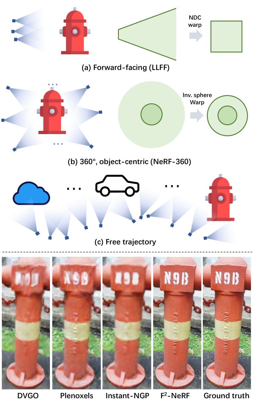
The research progress of novel view synthesis has advanced drastically in recent years since the emergence of the Neural Radiance Field (NeRF) [25, 43]. Once the training is done, NeRF is able to render high-quality images from novel camera poses. The key idea of NeRF is to represent the scene as a density field and a radiance field encoded by Multi-layer Perceptron (MLP) networks, and optimize the MLP networks with the differentiable volume rendering technique. Though NeRF is able to achieve photo-realistic rendering results, training a NeRF takes hours or days due to the slow optimization of deep neural networks, which limits its application scopes.

Recent works demonstrate that grid-based methods, such as Plenoxels [58], DVGO [39], TensoRF [6], and Instant-NGP [26], enable fast training a NeRF within a few minutes. However, the memory consumption of such grid-based representations grows in cubic order with the size of the scene. Though various techniques, such as voxel pruning [58, 39], tensor decomposition [6] or hash indexing [26], are proposed to reduce the memory consumption, these methods still can only process bounded scenes when grids are built in the original Euclidean space.

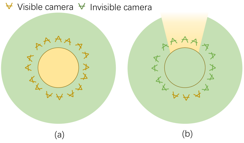
To represent unbounded scenes, a commonly-adopted strategy is to use a space-warping method that maps an unbounded space to a bounded space [25, 3, 62]. There are typically two kinds of warping functions. (1) For forward-facing scenes (Fig. 1 (a)), the Normalized Device Coordinate (NDC) warping is used to map an infinitely-far view frustum to a bounded box by squashing the space along the z-axis [25]; (2) For 360^∘ object-centric unbounded scenes (Fig. 1 (b)), the inverse-sphere warping can be used to map an infinitely large space to a bounded sphere by the sphere inversion transformation [3, 62]. Nevertheless, these two warping methods assume special camera trajectory patterns and cannot handle arbitrary ones. In particular, when a trajectory is long and contains multiple objects of interest, called free trajectories, as shown in Fig. 1 (c), the quality of rendered images degrades severely.

The performance degradation on free trajectories is caused by the imbalanced allocation of spatial representation capacity. Specifically, when the trajectory is narrow and long, many regions in the scenes are empty and invisible to any input views. However, the grids of existing methods are regularly tiled in the whole scene, no matter whether the space is empty or not. Thus, much representation capacity is wasted on empty space. Although such wasting can be alleviated by using the progressive empty-voxel-pruning [58, 39], tensor decomposition [6] or hash indexing [26], it still causes blurred images due to limited GPU memory. Furthermore, in the visible spaces, multiple foreground objects in Fig. 1 (c) are observed with dense and near input views while background spaces are only covered by sparse and far input views. In this case, for the optimal use of the spatial representation of the grid, dense grids should be allocated for the foreground objects to preserve shape details and coarse grids should be put in background space. However, current grid-based methods allocate grids evenly in the space, causing the inefficient use of the representation capacity.

To address the above problems, we propose F²-NeRF (Fast-Free-NeRF), the first fast NeRF training method that accommodates free camera trajectories for large, unbounded scenes. Built upon the framework of Instant-NGP [26], F²-NeRF can efficiently be trained on unbounded scenes with diverse camera trajectories and maintains the fast convergence speed of the hash-grid representation.

In F²-NeRF , we give the criterion on a proper warping function under an arbitrary camera configuration. Based on this criterion, we develop a general space-warping scheme called the perspective warping that is applicable to arbitrary camera trajectories. The key idea of perspective warping is to first represent the location of a 3D point ${\bf p}$ by the concatenation of the 2D coordinates of the projections of ${\bf p}$ in the input images and then map these 2D coordinates into a compact 3D subspace space using Principle Component Analysis (PCA) [52]. We empirically show that the proposed perspective warping is a generalization of the existing NDC warping [25] and the inverse sphere warping [62, 3] to arbitrary trajectories in a sense that the perspective warping is able to handle arbitrary trajectories while could automatically degenerate to these two warping functions in forward-facing scenes or 360^∘ object-centric scenes. In order to implement the perspective warping in a grid-based NeRF framework, we further propose a space subdivision algorithm to adaptively use coarse grids for background regions and fine grids for foreground regions.

We conduct extensive experiments on the unbounded forward-facing dataset, the unbounded 360^∘ object-centric dataset, and a new unbounded free trajectory dataset. The experiments show that F²-NeRF uses the same perspective warping to render high-quality images on the three datasets with different trajectory patterns. On the new Free dataset with free camera trajectories, our method outperforms baseline grid-based NeRF methods,while only using $\sim$12 minutes on training on a 2080Ti GPU.

2 Related Works

Novel view synthesis. Novel view synthesis (NVS) aims to synthesize novel view images from input posed images. The NVS problem has been extensively studied with lumigraph [5, 13] and light field functions [8, 16] to directly interpolate input images. To improve the quality of the synthesized image, many methods resort to an explicit 3D reconstruction of the scene via meshes [9, 44, 48, 53], voxels [14, 21, 22, 35], point clouds [1, 55], depth maps [10, 32, 33, 46], and multi-plane images (MPI) [12, 17, 24, 37, 45, 64], and then synthesize novel images with the help of these 3D reconstructions. F²-NeRF also aims to solve the NVS task but with a neural representation.

Neural scene representations. Since the emergence of NeRF [25, 2, 42], there have been intensive studies on neural representations for the tasks of novel view synthesis [25, 36, 43], relighting [4, 27, 61, 63], generalization to new scenes [60, 51, 20, 7, 49, 38], shape representation [23, 40, 26], and multi-view reconstruction [57, 50, 28, 56]. The representation can be either totally neural networks [25, 34, 11, 18, 30], or hybrid parametric encodings with space subdivisions [40, 23, 26, 19] for efficient training and inference. F²-NeRF also subdivides the scene for flexible space warping and uses the hybrid neural scene representation [26] for fast training and high-quality rendering.

Fast NeRF training with space warping. Recent works show that the training of NeRF can be accelerated significantly with grid-based representations [58, 6, 39, 26]. Instead of using a huge MLP network to predict the density and color, Plenoxels [58] directly store the density values and colors on a voxel grid. Instant-NGP [26], TensoRF [6] and DVGO [39] construct a feature grid and the density and compute the density and the color for a specific point from an interpolated feature vector using a tiny MLP network. However, these grids are regularly constructed in an axis-aligned manner and require additional space warping to represent unbounded scenes. There are two kinds of existing space warping functions, the NDC warping [25] for the forward-facing scenes and the inverse sphere warping [3, 2, 62] for the 360^∘ object-centric scenes. Both of these warping functions cannot handle long and narrow trajectories. In F²-NeRF , we propose a novel perspective warping to enable these fast grid-based methods to process arbitrary camera trajectories.

Large-scale Neural Radiance Fields. Recent works [47, 54, 41] managed to reconstruct the radiance field on a large-scale scene by decomposing the scene into blocks and separately training different NeRFs for different blocks. F²-NeRF aims at small-scale scenes with arbitrary camera trajectories, which has the potential to serve as the backbone NeRF of a single block in large-scale NeRFs.

Figure 2: A 2D example. (a) The gray regions at the orange points align with the image resolutions. (b) Axis-aligned grids in the original Euclidean space are not aligned with the camera rays.

3 Our Approach

Given a set of images $\{\mathcal{I}_{i}\}$ with arbitrary but known poses in an unbounded scene, the goal of F²-NeRF is to reconstruct a radiance field of the scene for the novel view synthesis task. In the following, we first give an overview of F²-NeRF .

3.1 Overview

In order to build a grid-based neural representation in an unbounded scene, a space warping function $F(\mathbf{x})$ is introduced to warp the unbounded space to a bounded region. In Sec. 3.2, we first analyze the mechanism of space warping and propose a novel perspective warping method. The proposed perspective warping subdivides whole the space under consideration into small regions, as shown in Sec. 3.3. Then, on the warp space, we build a grid-based neural representation in Sec. 3.4. Based on the built representation, we adopt the volume rendering [25] to render novel-view images.

Volume rendering with perspective warping. In order to render the color $\hat{c}$ for a pixel, we first apply a novel point sampling strategy, called the perspective sampling in Sec. 3.5, to sample points $\mathbf{x}_{i}$ on the camera ray emitting from the pixel. Then, these sampled points are warped by the perspective warping to the warp space, and the density $\sigma_{i}$ and the color $c_{i}$ on sampled points are computed from the neural representation built on the warp space. Finally, we composite the colors to compute the pixel color $\hat{c}$ by

$$\hat{c}=\sum_{i}{T_{i}\alpha_{i}c_{i}},$$ (1)

where $T_{i}=\prod_{j=0}^{i-1}(1-\alpha_{j})$ is the accumulated transmittance and $\alpha_{i}=1-\exp(-\delta_{i}\sigma_{i})$ is the opacity of the point.

3.2 Perspective warping

It has been demonstrated that space warping functions, such as the NDC warping [25] and the inverse sphere warping [62, 3], are effective for rendering unbounded scenes. In this section, we start with a 2D intuitive analysis of why a space warping method is effective.

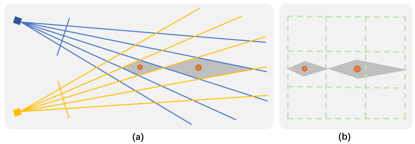
2D analysis. First, let us consider a simple case in the 2D space as shown in Fig. 2 (a). In this setting, two 2D cameras project the points from 2D space onto their 1D image planes. Consider the two orange points in the figure. The gray rhombuses are the irregular grids formed by camera rays and the gray regions are the smallest distinguishable region due to the limited resolution of the two cameras. However, a vanilla grid-based representation consists of axis-aligned regular grids as shown in Fig. 2 (b), which is not aligned with the gray rhombuses. Moreover, such misalignment becomes more severe as the distance from the cameras increases. The key requirement for space warping is that we need to warp the original Euclidean space and build axis-aligned grids in the warp space so that these grids are aligned with the camera rays. Clearly, in this 2D case, a proper warping function $F(\mathbf{x}):\mathbb{R}^{2}\rightarrow\mathbb{R}^{2}$ can be constructed by $F(\mathbf{x})=(C_{1}(\mathbf{x}),C_{2}(\mathbf{x}))$, where $C_{1}(\mathbf{x})$ and $C_{2}(\mathbf{x})$ denotes the 1D image coordinates of projecting $\mathbf{x}$ onto the camera 1 and camera 2 respectively. Then, the axis-aligned grids built on the $F(\mathbf{x})$ space will exactly align with camera rays.

Proper space warping. Based on the 2D analysis above, we define a proper space warping function as follows.

Definition 1

Given a region $S$ in the 3D Euclidean space and a set of cameras $\{C_{i}|i=1,2,...,n_{c}\}$ which are visible to $S$, a warping function $F:\mathbb{R}^{3}\to\mathbb{R}^{3}$ is called a proper warping function, if for any two points $\mathbf{x}_{1},\mathbf{x}_{2}\in S$, the distance between these two points in the warp space equals to the sum of distances between these two points on all visible cameras, i.e. $\|F(\mathbf{x}_{1})-F(\mathbf{x}_{2})\|_{2}^{2}=\sum_{i}^{n}\|C_{i}(\mathbf{x}_{1})-C_{i}(\mathbf{x}_{2})\|_{2}^{2}$.

Clearly, the warping function $F(\mathbf{x})=(C_{1}(\mathbf{x}),C_{2}(\mathbf{x}))$ in the 2D toy example is a proper 2D warping function. Note that whether a warping function is proper or not is a local property, which only relates to the visible cameras.

Figure 3: Our perspective warping method.

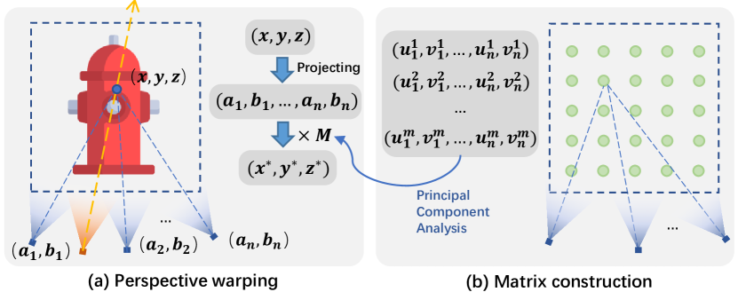
3D perspective warping. Given the region $S$ and the cameras $C_{i}$, we now would like to construct a proper 3D warping function $F(\mathbf{x}):\mathbb{R}^{3}\rightarrow\mathbb{R}^{3}$. We begin with an observation that the function $\mathbf{y}=G(\mathbf{x})=[C_{1}(\mathbf{x}),...,C_{n_{c}}(\mathbf{x})]:\mathbb{R}^{3}\to\mathbb{R}^{2n_{c}}$ which maps the 3D point to its projected coordinates on all $n$ cameras $C_{i}$ is a proper warping function because this is a trivial construction based on the definition of a proper warping function. However, what we want to construct eventually is a function that maps a 3D space to a 3D space. Hence, we consider constructing an approximately proper warping function $F$ with the following formulation.

Problem 1

Let $\{\mathbf{x}_{j}|j=1,2,...,n_{p}\}$ denote $n_{p}$ evenly-sampled points in the local region $S$ of the original Euclidean space, we want to find a projection matrix $M\in\mathbb{R}^{3\times 2n_{c}}$ that maps the coordinate $\mathbf{y}_{j}=G(\mathbf{x}_{j})\in\mathbb{R}^{2n_{c}}$ to $\mathbf{z}_{j}\in\mathbb{R}^{3}$ by $\mathbf{z}_{j}=M\mathbf{y}_{j}$, so that $M$ minimizes $\sum_{j}^{K}\|M^{\intercal}\mathbf{z}_{j}-\mathbf{y}_{j}\|_{2}^{2}$

In comparison with Definition 1, Problem 1 makes two relaxations. First, we only consider the distances between sampled points $x_{i}\in S$ in Problem 1 while Definition 1 considers arbitrary point pairs. Second, we apply a projection matrix such that the distances between $\mathbf{y}_{i}$ are preserved as much as possible. It can be shown that the solution to this problem is exactly the Principle Component Analysis (PCA) [52] on the set of projection points $\{\mathbf{y}_{j}\}$. The matrix $M$ is constructed from the first three eigenvectors of the covariance matrix of $\{\mathbf{y}_{j}\}$. Therefore, the proposed perspective warping function is $F(\mathbf{x})=MG(\mathbf{x})$, as shown Fig. 3. In our implementation, we perform a post normalization on $F(\mathbf{x})$ to make the resulting points $\{\mathbf{z}_{j}\}$ in the warp space located around the origin, which is introduced in details in the supplementary material.

Figure 4: Visualization of the effect of perspective warping. (a) Points in the original Euclidean space. (b) Points in the warp space and the corresponding camera angles.

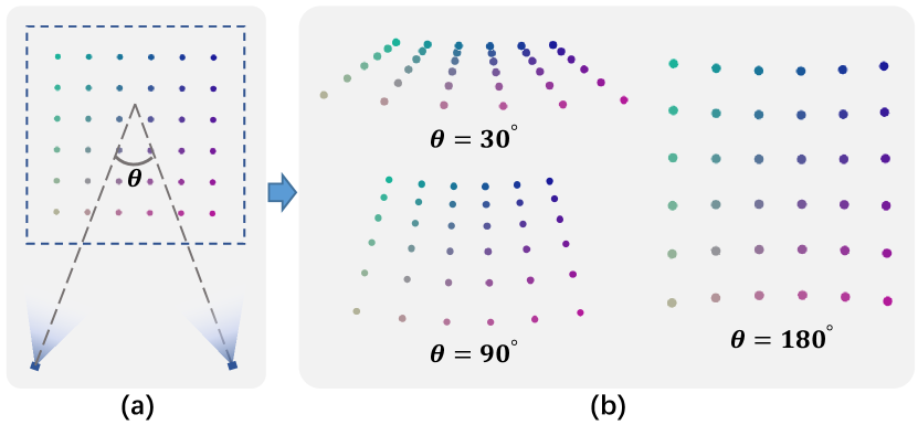
Intuition of $F(\mathbf{x})$. $F(\mathbf{x})$ maps the region $S$ in the original space to a region around the origin of the warp space. Fig. 4 shows the perspective warping with different angles between two neighboring cameras. As we can see, when the angle $\theta$ is small, the space is squashed more on the far region, which is a similar behavior to the NDC warping. In this case, the perspective warping reduces to the NDC warping if all the cameras are forward-facing. When the angle becomes larger, the warp space is more similar to the original Euclidean space.

Figure 5: Inverse sphere warping. (a) The inner unit sphere are visible to all cameras around. Thus, the warp space is a Euclidean space, which corresponds to the 180^∘ case of perspective warping in Fig. 4. (b) The outer space is only visible to a part of cameras. The outer space uses an NDC warping, which corresponds to the 30^∘ case of perspective warping in Fig. 4.

Figure 6: Pipeline of F²-NeRF . (a) Given a large region of interest, we subdivide the space according to the input view frustums. (b) For each sub-region, we construct a perspective warping function based on the visible cameras. The densities and colors are decoded from the scene feature vectors fetched from the same hash table (d) but using different hash functions (c).

Relationship with inverse sphere warping. We empirically show that inverse sphere warping [62, 3] is also a handcrafted approximation of our perspective warping function. As shown in Fig. 5 (a), the warp space of the inverse sphere warping for the inner unit sphere is simply the original Euclidean space because all the cameras around are visible to this unit sphere, which corresponds to the $180^{\circ}$ case in Fig. 4 of the perspective warping. The outer space (Fig. 5 (b)) is only visible from a few far cameras and thus is warped similarly as the NDC warping, which corresponds to the $30^{\circ}$ case in Fig. 4 of the perspective warping.

3.3 Space subdivision

In order to apply the perspective warping function $F(\mathbf{x})$, we need to specify $n_{c}$ cameras onto which we project the point $\mathbf{x}$. According to Definition 1, the properness of the warping function is a local property which only relates the visible cameras for the point $\mathbf{x}$. However, for a free trajectory like Fig. 1 (c), visible cameras for different regions are different. This motivates us to adaptively subdivide the space into different regions such that the visible cameras used in $F(\mathbf{x})$ are the same inside a region but are different across regions. In this case, in each subdivided region $S_{i}$, a warping function $F_{i}(\mathbf{x})$ is applied to map $S_{i}$ to the warp space.

Subdivision strategy. We adopt an octree data structure to store the subdivided regions, which enables us to quickly search for a region and retrieve visible cameras. To construct the octree, we begin with an extremely large bounding box as the root node. Here the box size is $512$ times the bounding box size of all camera centers, which is able to contain extremely far-away sky or other objects. Then, starting from the octree root node, we perform a check-and-subdivide procedure. Specifically, on a tree node with $s$ as the side length, we retrieve all visible cameras whose view frustums intersect with this node. Then, if there is any visible camera center whose distance $d$ to the node center is $d\leq\lambda s$, where $\lambda$ is preset to 3, the node is subdivided into 8 child nodes with side length of $s/2$. Otherwise, the current node is small enough and we stop subdividing it and mark it as a leaf node. For each subdivided child node, we further check the distance and repeat this procedure until we get all $n_{l}$ leaf nodes $\{S_{i}|i=1,2,...,n_{l}\}$ as shown in Fig. 6 (a). Each leaf node is treated as the region $S$ in Problem 1, and for those regions that are visible by more than $n_{c}=4$ cameras, we further select $n_{c}$ visible cameras by making the minimal pair-wise distance of the selected cameras as large as possible. A more detailed description of the camera selection strategy can be found in the supplementary material. By applying the warping function $F_{i}$, each leaf node is mapped to a region around the origin of its warp space.

3.4 Scene representation

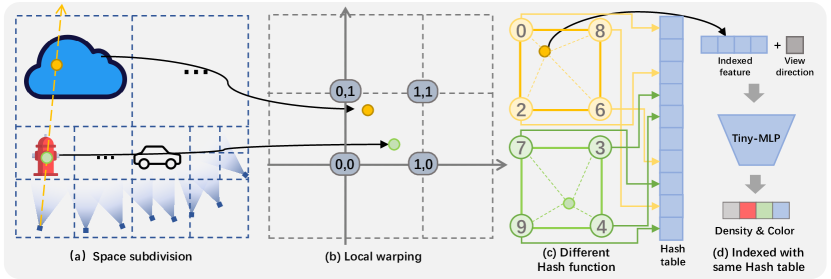
In this section, we will introduce how to build our grid-based scene representation on the warp space, which allows color and density computation for a given point in the warp space. Since the warping functions are different for different leaf nodes, we actually have $n_{l}$ different warp spaces. A naive solution would be to build $n_{l}$ different grid representations on each warp space. However, this would cause the number of parameters to grow with the number of leaf nodes. To limit parameter number, we suppose that all warping functions map different leaf nodes to the same warp space and build a hash-grid representation [26] on the warp space with multiple hash functions as shown in Fig. 6.

Hash grid with multiple hash functions. Sharing the same warp space for different leaf nodes will inevitably lead to conflicts, which means two different points in two leaf nodes with different densities and colors are mapped to the same point in the warp space. In the original Instant-NGP [26], there is only one hash function to compute hash values for grid vertices. Here, we use different hash functions for different leaf nodes to alleviate the conflict problem. Specifically, for a point $\mathbf{x}$ in the $i$-th leaf node, we map it to $\mathbf{z}=F_{i}(\mathbf{x})$ in the warp space and find $z$’s eight neighboring grid vertices $\hat{\mathbf{v}}$ with integer coordinates. Then, we compute a hash value for each vertex $\hat{\mathbf{v}}$ by a hash function conditioned on the leaf node index $i$ as follows

$${\rm Hash}_{i}(\hat{\mathbf{v}})=\left(\bigoplus_{k=1}^{3}\hat{\mathbf{v}}_{k}\pi_{i,k}+\Delta_{i,k}\right)\mod L,$$ (2)

where $\bigoplus$ denotes the bitwise xor operation, and both $\left\{\pi_{i,k}\right\}$ and $\left\{\Delta_{i,k}\right\}$ are random large prime numbers, which are fixed for a specific leaf node, $k=1,2,3$ means the index of $x,y,z$ coordinate of the warp space, $L$ is the length of the hash table. The computed hash value will be used in indexing the hash table to retrieve a feature vector for the vertex $\hat{\mathbf{v}}$ and then the feature vector of the point $z$ is trilinearly-interpolated from 8 vertex feature vectors. Finally, the feature vector of $z$ and the view direction $\mathbf{d}$ are fed into a tiny MLP network to produce color and density for the point $z$, as shown in Fig. 6 (d).

Intuition of Eq. 2. Using different numbers $\pi_{i,k}$ and different offsets $\Delta_{i,k}$ leads to different hash functions in Eq. 2. We use an example in Fig. 6 to show how Eq. 2 works: The green point and the yellow point in two different leaf nodes (Fig. 6 (a)) are mapped by two different warping functions to the same warp space (Fig. 6 (b)). Suppose that both points reside in the same voxel of the warp space. Although the coordinates of their neighboring vertices are the same, the two points will use different hash functions Eq. 2 to compute different hash values for these neighboring vertices (Fig. 6 (c)). Then, the computed hash values will be used in indexing the same hash table to retrieve feature vectors (Fig. 6 (d)). In this case, two points from different leaf nodes share the same neighboring vertices in the warp space but retrieve different vertex feature vectors, which greatly reduces the probability of conflicts. Though some conflicts still remain, they can naturally be resolved by the tiny MLP during the optimization process as observed by Instant-NGP [26].

3.5 Perspective sampling

A proper warping function $F$ also gives us a guideline for sampling points on rays in volume rendering. According to Definition 1, the distance between two points in the proper warp space equals the sum of distances between two projected points on image planes. In this case, by uniformly sampling the points in the warp space, we get a non-uniform sampling in the original Euclidean space but an approximately uniform sampling on images, which improves the sampling efficiency and brings more stable convergence. Specifically, considering a sample point $\mathbf{x}_{i}=\mathbf{o}+t_{i}\mathbf{d}$ where $\mathbf{o},\mathbf{d}$ are the camera origin and direction respectively, we first compute the Jacobian matrix $J_{i}\in\mathbb{R}^{3\times 3}$ of the perspective warping function $F$ at $\mathbf{x}_{i}$. Then, the next sample point $\mathbf{x}_{i+1}=\mathbf{x}_{i}+\frac{l}{\|J_{i}\mathbf{d}\|_{2}}\mathbf{d}$, where $l$ is a preset parameter controlling the sampling interval and we make a linear approximation here as discussed in the supplementary material.

3.6 Rendering with perspective warping

Based on the descriptions above, we now summarize the rendering procedure in two stages: the preparation stage and the actual rendering stage. (1) In the preparation stage, we subdivide the original space according to the view frustums of the cameras (Sec. 3.3), and construct the local warping functions based on the selected cameras for each sub-region (Sec. 3.2). (2) In the actual rendering stage, we follow the framework of volume rendering to render a pixel color, by sampling points on the camera ray (Sec. 3.5) and conducting weighted accumulation of the sampled colors (Sec. 3.1). The sampled densities and colors are fetched from the multi-resolution hash grid (Sec. 3.4).

3.7 Training

The training loss is defined as

$$\mathcal{L}=\mathcal{L}_{recon(c(r),c_{{\rm gt}})}+\lambda_{\rm Disp}\mathcal{L}_{\rm Disp}+\lambda_{\rm TV}\mathcal{L}_{\rm TV},$$ (3)

where $\mathcal{L}_{recon(c(r),c_{\rm gt})}=\sqrt{(c(r)-c_{{\rm gt}})^{2}+\epsilon}$ is a color reconstruction loss [3] with $\epsilon=10^{-4}$. $\mathcal{L}_{\rm Disp}$ and $\mathcal{L}_{\rm TV}$ are two regularization losses. The first is a disparity loss $\mathcal{L}_{\rm Disp}$ that encourages the disparity (inverse depth) not excessively large, which is useful to reduce the floating artifacts. The second is a total variance loss [31] $L_{\rm TV}$ that encourages the points at the borders of two neighboring octree nodes $i,j$ to have similar densities and colors. For all losses, we provide more details in the supplementary material.

4 Experiments

Figure 7: Trajectories of “Sky” and “Stair” in the Free dataset.

Figure 8: Visual comparison on the Free dataset.

4.1 Experimental Settings

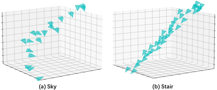
Datasets. We use three datasets for our evaluation. (1) A new unbounded dataset with free trajectories that we collected (called the Free dataset). The Free dataset contains seven scenes. Each scene has a narrow and long input camera trajectory and multiple focused foreground objects, which is extremely challenging to build a neural representation for the NVS task. Two of these trajectories are shown in Fig. 7; (2) LLFF dataset [24], which contains eight real unbounded forward-facing scenes with complex geometries; and (3) NeRF-360-V2 dataset [3], which contains seven unbounded 360-degree inward-facing outdoor and indoor scenes. For all the datasets, we follow the commonly-adopted settings that set one of every eight images as testing images and the other as the training set. We use three metrics, PSNR, SSIM, and LPIPS_VGG, for evaluation.

Baselines. We compare F²-NeRF with the state-of-the-art fast NeRF training methods, the voxel-based methods (1) DVGO [39], (2) Plenoxels [58] and the hash-grid based method (3) Instant-NGP [26]. We also report the results of MLP-based NeRF methods including NeRF++ [62], mip-NeRF [2], and mip-NeRF-360 [3]. Note that both F²-NeRF and Instant-NGP [26] are trained for 20k steps with the same batch size but we adopt a LibTorch [29] implementation while Instant-NGP uses a CUDA implementation, which is faster (6min) than ours (13min). All training times are evaluated on a single 2080Ti GPU. Implementation details of F²-NeRF are included in the supplementary material.

Warping functions. Different warping functions are adopted for baseline methods on different datasets. On the LLFF dataset, all baselines use the NDC warping function, and on both the Free dataset and the NeRF-360-V2 dataset, all baseline methods use the inverse sphere warping function, except Instant-NGP. In the Instant-NGP, we follow the official implementation to enlarge the ray marching bounding box to represent backgrounds and carefully tune the scale parameters on different scenes to achieve the best performance. In comparison, F²-NeRF always uses the perspective warping for all datasets.

Method	Tr. time	PSNR$\uparrow$	SSIM$\uparrow$	LPIPS(VGG)$\downarrow$
NeRF++ [62]	hours	23.47	0.603	0.499
mip-NeRF-360 [3]	hours	27.01	0.766	0.295
mip-NeRF-360short	30m	22.04	0.537	0.586
Plenoxels [58]	25m	19.13	0.507	0.543
DVGO [39]	21m	23.90	0.651	0.455
Instant-NGP [26]	6m	24.43	0.677	0.413
F2-NeRF	12m	26.32	0.779	0.276

Table 1: Results on the Free dataset. In mip-NeRF-360_short, we early stop the training to make them finished in 30 minutes. Training times are evaluated on a 2080ti GPU.

4.2 Comparative studies

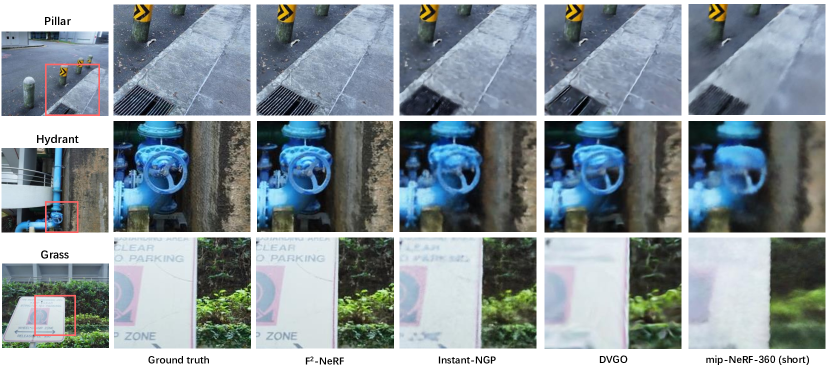
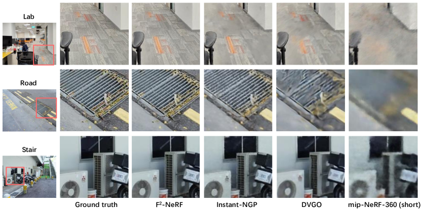
We report the quantitative comparisons on the Free dataset in Table 1. F²-NeRF achieves the best rendering quality among all the fast-training NeRFs. The results for qualitative comparison are shown in Fig. 8. The synthesized images of DVGO [39] and Plenoxels [59] are blurred due to their limited resolutions to represent such a long trajectory. The results of Instant-NGP look sharper but are not clear enough due to its unbalanced scene space organization. In comparison, F²-NeRF takes advantage of the perspective warping and the adaptive space subdivision to fully exploit the representation capacity, which enables F²-NeRF to produce better rendering quality. Meanwhile, we find that training a mip-NeRF-360 on the Free dataset for a long time is also able to render clear images. The reason is that during the training process, the large MLP networks used by mip-NeRF-360 are able to gradually concentrate on foreground objects and adaptively allocate more capacity to these foreground objects. However, these MLP networks have to spend a long training time for convergence on the Free Trajectory dataset. With a short training time (30 minutes), the results of mip-NeRF-360 contain many foggy artifacts.

We also evaluate our method on the widely-used unbounded forward-facing dataset (LLFF) and 360^∘ object-centric dataset (NeRF-360-V2) to show the compatibility of the perspective warping with these two kinds of specialized camera trajectories. On both datasets, F²-NeRF achieves comparable results to the other fast NeRF methods. Note these baseline fast NeRF methods adopt the specially-designed NDC warping or inverse sphere warping for the LLFF dataset or the NeRF-360-V2 dataset while F²-NeRF always uses the same perspective warping for all datasets. This demonstrates the compatibility of the perspective warping with different trajectories.

Method	Tr. time	PSNR$\uparrow$	SSIM$\uparrow$	LPIPS(VGG)$\downarrow$
NeRF++ [62]	hours	26.21	0.729	0.348
mip-NeRF-360 [2]	hours	28.94	0.837	0.208
Plenoxels [58]	22m	23.35	0.651	0.471
DVGO [39]	16m	25.42	0.695	0.429
Instant-NGP [26]	6m	26.24	0.716	0.404
F2-NeRF	14m	26.39	0.746	0.361

Table 2: Results on the NeRF-360-V2 dataset.

Method	Tr. time	PSNR$\uparrow$	SSIM$\uparrow$	LPIPS(VGG)$\downarrow$
NeRF [25]	hours	26.50	0.811	0.250
mip-NeRF [2]	hours	26.60	0.814	0.246
Plenoxels [58]	17m	26.29	0.839	0.210
DVGO [39]	11m	26.34	0.838	0.197
TensoRF [6]	48m	26.73	0.839	0.204
Instant-NGP [26]	6m	25.09	0.758	0.267
F2-NeRF	13m	26.54	0.844	0.189

Table 3: Results on the LLFF dataset.

4.3 Ablation studies

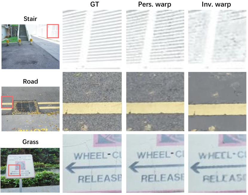
We conduct ablation studies on the “pillar” from the Free dataset. In the ablation studies, we use the multi-resolution hash grid [26] as the scene representation and change the warping functions and the sampling strategies. The warping functions include the inverse sphere warping (Inv. warp), the perspective warping (Pers. warp), and no warping (w/o warp). In the implementation of inverse sphere warping on the Free dataset, we use the bounding sphere of all camera positions as the foreground inner sphere and treat the space outside the sphere as backgrounds. For the point sampling strategies, we consider sampling by disparity (inverse-depth) (Disp. Sampling) used in mip-NeRF-360 [3], sampling by the exponential function (Exp. Sampling) used in Instant-NGP [26], and our perspective sampling (Sec. 3.5). The quantitative results are shown in Table 4 and some qualitative results are shown in Fig. 9.

As shown in Table 4, the basic model (A) without space warping and using disparity sampling performs worst. The model (B) with Inv. warping improves the performances, which shows better compatibility with unbounded scenes compared with no warping (A). The model (C) replaces the disparity sampling with the exponential sampling, which makes the results better. The model (D) uses the proposed perspective warping, whose performance increases drastically compared to the inverse sphere warping. This demonstrates the effectiveness of our perspective warping on free trajectories. The model (E) further applies perspective sampling, which produces the best performance.

Figure 9: Visual comparison of different warping techniques. Our perspective warping renders more clear images than inverse sphere warping [3].

Setting	PSNR$\uparrow$	SSIM$\uparrow$	LPIPS$\downarrow$
A) w/o warp + Disp. sample	26.81	0.693	0.385
B) Inv. warp + Disp. sample	27.09	0.711	0.358
C) Inv. warp + Exp. sample	27.86	0.751	0.289
D) Pers. warp + Exp. sample	28.65	0.796	0.221
E) Pers. warp + Pers. sample	28.76	0.798	0.219

Table 4: Ablation study on the “pillar” scene of the Free dataset. F²-NeRF with perspective warping and sampling achieves the best quantitative results.

5 Conclusion

In the NVS task of unbounded scenes, previous NeRF methods mainly rely on the NDC warping or the inverse sphere warping to process the forward-facing camera trajectory or the 360^∘ object-centric trajectory. In this paper, we conduct an in-depth analysis of the space warping function and propose a novel perspective warping, which is able to handle arbitrary input camera trajectories. Based on the perspective warping, we develop a novel F²-NeRF in the grid-based NeRF framework. Extensive experiments demonstrate that the proposed F²-NeRF is able to render high-quality images with arbitrary trajectories while only requiring a few minutes of training time.

Potential negative societal impact. F²-NeRF can be possibly used for misleading fake image generation.

Acknowledgement. This study is supported by the Ministry of Education, Singapore, under its MOE AcRF Tier 2 (MOE-T2EP20221-0012), NTU NAP, and under the RIE2020 Industry Alignment Fund – Industry Collaboration Projects (IAF-ICP) Funding Initiative, as well as cash and in-kind contribution from the industry partner(s). Lingjie Liu and Christian Theobalt have been supported by the ERC Consolidator Grant 4DReply (770784).

- Supplementary -

A Additional Implementation Details

Figure 10: Camera rectification.

A.1 Camera processing

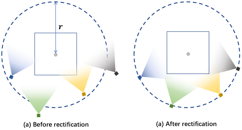
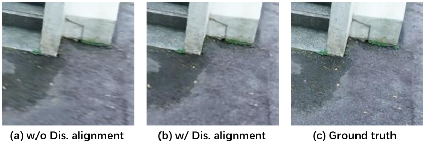
Camera rectification. After the procedure of space-subdivision (Sec 3.3 of the main paper), for each sub-region $S$, we obtain a set of visible cameras whose view frustums intersect with $S$. We note that visible cameras are not suitable to be directly used in computing of the perspective warping, because some cameras do not fully cover the region and look at the region as shown in Fig. 10(a). Thus, we propose an empirical but effective camera rectification strategy, that we rotate the camera view directions to make them look at the center of the region $S$. This simple strategy helps ensure most points inside $S$ can be warped to meaningful coordinates. Moreover, we find that aligning their distances to the center of $S$ with the same distance $r$ can help improve the rendering quality, as shown in Fig. 12. Here $r$ is empirically set as the mean distance to the region center among the 1/4 nearest visible cameras.

Camera selection. When the number of visible cameras is larger than $n_{c}=4$, we select a subset of the visible cameras for better computational efficiency. We select the cameras based on the farthest point sampling: First, we randomly select a camera as the seed, and then we repeatedly add the farthest visible camera for $n_{c}-1$ times.

Figure 11: The effect of distance alignment.

A.2 Construction of $M$

In this section, we give a detailed description of how we construct the matrix $M$ for our perspective warping.

Principal component analysis. Given the region $S$ with the selected cameras, we first uniformly sample $n=32^{3}$ points $\{{\bf x}_{i}\}$ inside $S$. Then, we project the points to the selected cameras, concatenate the projected coordinates, and obtain the high-dimensional coordinates $\left\{\left[C_{1}({\bf x}_{i}),...,C_{n_{c}}({\bf x}_{i})\right]=\left[u_{1}^{i},v_{1}^{i},...,u_{n_{c}}^{i},v_{n_{c}}^{i}\right]\right\}.$ These coordinates are formed in a coordinate matrix $K\in\mathbb{R}^{2n_{c}\times n}$, then we compute the covariance matrix $Q=(K-\overline{K})(K-\overline{K})^{\top}$, where $\overline{K}$ is the mean coordinate of all projected coordinates. By eigendecomposition, we obtain the matrix $M^{\prime}\in\mathbb{R}^{3\times 2n_{c}}$ formed by the eigenvectors with the first three largest eigenvalues. The matrix $M^{\prime}$ defines the directions of the projection axes.

Figure 12: The Jacobian matrices among different spaces.

Computing the axis length. After the matrix $M^{\prime}\in\mathbb{R}^{3\times 2n_{c}}$ is found, we now need to perform a post normalization by scaling each axis. Specifically, we would like to find three proper scale parameters $\{s_{1},s_{2},s_{3}\}$, and $M=SM^{\prime}$, where $S\in\mathbb{R}^{3}$ is the diagonal matrix formed by $\{s_{1},s_{2},s_{3}\}$. The key idea of these scaling parameters is that we expect the unit length in the warp space can be approximately aligned with the unit length in the image space. More specifically, for each axis in the warp space, when a point moves along the axis by a unit length, we expect the maximum spatial transition of all image coordinates to be approximately a pixel length.

We take a point ${\bf x}$ inside the region $S$ for example. Let us denote the Jacobian matrix from the original space to the image space as $J_{O\rightarrow I}\in\mathbb{R}^{3\times 2n_{c}}$ derived from the image projection function, and the Jacobian matrix from the image space to the warp space as $J_{I\rightarrow W}=M=SM^{\prime}$. Our target is to compute the Jacobian matrix $J_{W\rightarrow I}\in\mathbb{R}^{2n_{c}\times 3}$ and put a constraint that the maximum value of each column vector of $J_{W\rightarrow I}$ equals one. Note $J_{W\rightarrow I}$ may not be directly computed by inverting $J_{I\rightarrow W}$, which is not a square matrix. Alternatively, we present it by $J_{W\rightarrow I}=J_{O\rightarrow I}J_{W\rightarrow O}$, which can be further represented by

$$\begin{split}J_{W\rightarrow I}&=J_{O\rightarrow I}J_{O\rightarrow W}^{-1}\\ &=J_{O\rightarrow I}(J_{I\rightarrow W}J_{O\rightarrow I})^{-1}\\ &=J_{O\rightarrow I}(SM^{\prime}J_{O\rightarrow I})^{-1}\\ &=J_{O\rightarrow I}(M^{\prime}J_{O\rightarrow I})^{-1}S^{-1}.\end{split}$$ (4)

What we expect is that the maximum value of each column vector of $J_{W\rightarrow I}$ equals one. This constraint can solve the values of $\{s_{1},s_{2},s_{3}\}$ for the example point ${\bf x}$. For all the sampled points $\{{\bf x}_{i}\}$, we take the average values of $\{s_{1},s_{2},s_{3}\}$ for our final scale parameters.

A.3 Perspective sampling

As stated in the main paper (Sec 3.5), when sampling points in ray marching, we perform uniform sampling on the warp space, and we get a non-uniform sampling in the original space. To be specific, for the current sample point ${\bf x}_{i}={\bf o}+t_{i}{\bf d}$, we expect to find the next sample point ${\bf x}_{i+1}={\bf x}_{i}+\delta_{i}{\bf d}$, such that $\|F({\bf x}_{i+1})-F({\bf x}_{i})\|_{2}=l$. Here $l$ is the parameter controlling sample density and we empirically set $l=\sqrt{3}$, i.e., the diagonal length of the unit cube in the warp space [26]. To compute the marching step $\delta_{i}$ in the original space efficiently, we perform a linear approximation that

$$F({\bf x}_{i+1})\approx F({\bf x}_{i})+\delta_{i}\cdot J_{i}{\bf d},$$ (5)

Where $J_{i}$ is the Jacobian matrix at ${\bf x}_{i}$ from the original space to the warp space. Hence, the distance between $F({\bf x}_{i+1})$ and $F({\bf x}_{i})$ is approximated by $\delta_{i}\|J_{i}{\bf d}\|_{2}$. We let it equals $l$ and get $\delta_{i}=\frac{l}{\|J_{i}{\bf d}\|_{2}}$.

A.4 Loss functions

As described in the main paper, the loss of training is defined as

$$\mathcal{L}=\mathcal{L}_{recon(c(r),c_{{\rm gt}})}+\lambda_{\rm Disp}\mathcal{L}_{\rm Disp}+\lambda_{\rm TV}\mathcal{L}_{\rm TV},$$ (6)

where the first term $\mathcal{L}_{recon(c(r),c_{\rm gt})}=\sqrt{(c(r)-c_{{\rm gt}})^{2}+\epsilon}$ is a color reconstruction loss [3] with $\epsilon=10^{-4}$, and the last two terms are the regularization losses.

The disparity loss $\mathcal{L}_{\rm Disp}$ of the sampled rays is defined by

$$\mathcal{L}_{\rm Disp}=\frac{1}{n_{r}}\sum_{k}{\rm disp}_{k}^{2},$$ (7)

where the disparity of a ray is computed by the weighted sum of the sampled inverse distance that ${\rm disp}=\sum_{i}w_{i}\frac{1}{t_{i}}$, and $\{w_{i}\}$ are the weights computed by volume rendering.

The aim of total variation loss $\mathcal{L}_{\rm TV}$ is to encourage the border points of two neighboring octree nodes to have similar densities and colors. To achieve this goal, in each training iteration, we randomly sample $n_{b}=8192$ points on the borders of the octree nodes, then the loss is defined by

$$\mathcal{L}_{\rm TV}=\frac{1}{n_{b}}\sum_{k}\|{\rm feat}_{0}^{k}-{\rm feat}_{1}^{k}\|_{2}^{2}.$$ (8)

Here, for each sample point $k$, ${\rm feat}_{0}^{k}$ and ${\rm feat}_{1}^{k}$ are the feature vectors fetched from the hash table using two different functions conditioned on its two neighboring octree nodes.

In LLFF dataset we set $\lambda_{\rm Disp}=2.5\times 10^{-4},\lambda_{\rm TV}=10^{-1}$, and in Free dataset and NeRF-360-V2 dataset we set $\lambda_{\rm Disp}=10^{-3},\lambda_{\rm TV}=10^{-1}$.

A.5 More implementation details

Architecture details. We follow a similar setting to Instant-NGP [26] and use the hash table with $16$ levels, and each level contain $2^{19}$ feature vectors with dimension of $2$. The fetched hash feature vectors of size 32 are fed to a tiny MLP with one hidden layer of width 64, to get the scene features and the volume densities, then, the scene features are concatenated with the spherical harmonics encoding of view directions and are fed to another rendering MLP with two hidden layers of width 64 to get the RGB colors.

Training details. We follow Instant-NGP [26] and set the fixed batch size of point samples as 256k while the batch size of rays is dynamic, depending on the average sampled points on rays. We train the parameters with Adam optimizer [15], whose learning rate linearly grows from zero to $1\times 10^{-1}$ in the first 1k steps and the decay to $10^{-2}$ at the end of training with cosine scheduling. For all the scenes in the experiments, we train F²-NeRF for 20k steps. We implement F²-NeRF using LibTorch [29]. The training time depends on the scene’s complexity, and for most cases, it is between 10 minutes and 15 minutes on a single Nvidia 2080Ti GPU.

Figure 13: Different warp coordinates.

B Connection to NDC warping and Inv. sphere warping

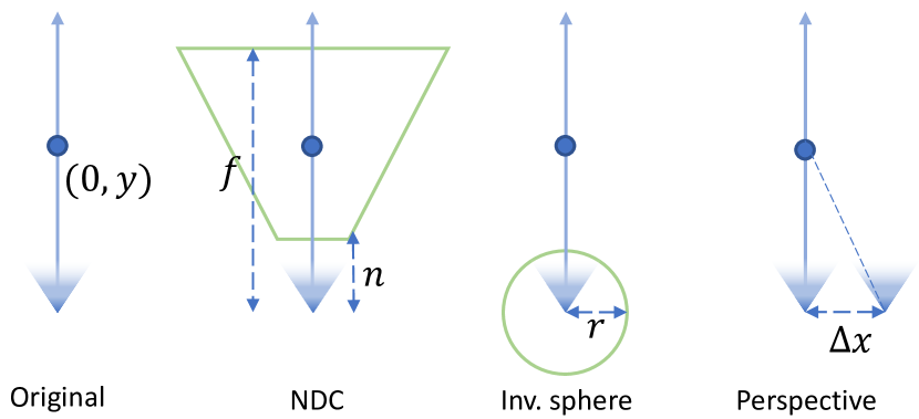
In the main paper, we intuitively show the connection of our proposed perspective warping to NDC warping and inverse sphere warping. Here we mathematically analyze the connections using two forward-facing 1D cameras that project 2D points onto their 1D camera plane as shown in Fig. 13. The proper perspective warping utilizes the image coordinates of two cameras as the warping coordinates. Thus, the point with coordinate $(0,y)$ in the original Euclidean space will be mapped to $(0,-\frac{\Delta_{x}}{y})$ in the warping space. Meanwhile, the coordinates of this point in the NDC space and inverse sphere space are $(0,\frac{f+n}{f-n}-\frac{2fn}{f-n}\cdot\frac{1}{y})$ and $(0,2-\frac{r}{y})$ respectively, where $n,f$ are preset near-far depth and $r$ is preset sphere radius. When $\Delta_{x}=\frac{2fn}{f-n}$ or $\Delta_{x}=r$, the perspective warping is equivalent to NDC warping or inverse sphere warping with a constant offset. However, theoretically proving such connections in general cases of the 3D space is very complex since it involves sampling points and PCA analysis on sample points.

C Additional Experimental Results

C.1 Training for longer steps

We provide quantitative results on training F²-NeRF and instant-NGP for a longer time on the Free dataset (Table 5) and NeRF-360-V2 dataset (Table 6). When trained for a longer time, F²-NeRF and Instant-NGP can obtain better rendering quality. As shown in Table 5, on the Free dataset, training Instant-NGP for a longer time (15m, 50k steps) does not achieve better rendering quality than F²-NeRF (12m, 20k steps). Moreover, increasing the hash table size from $2^{19}$ to $2^{20}$ helps improve the performance of F²-NeRF on the Free dataset (F²-NeRF _50k-large).

Method	Tr. time	PSNR$\uparrow$	SSIM$\uparrow$	LPIPS(VGG)$\downarrow$
Instant-NGP20k	6m	24.43	0.677	0.413
Instant-NGP50k	15m	25.07	0.703	0.376
F2-NeRF 20k	12m	26.32	0.779	0.276
F2-NeRF 50k	30m	26.85	0.811	0.235
F2-NeRF 50k-large	36m	27.19	0.833	0.204

Table 5: Training Instant-NGP and F²-NeRF for longer time on the Free dataset.

Method	Tr. time	PSNR$\uparrow$	SSIM$\uparrow$	LPIPS(VGG)$\downarrow$
Instant-NGP20k	6m	26.24	0.716	0.404
Instant-NGP50k	17m	26.55	0.733	0.382
F2-NeRF 20k	14m	26.39	0.746	0.361
F2-NeRF 50k	33m	26.92	0.771	0.333

Table 6: Training Instant-NGP and F²-NeRF for longer time on the NeRF-360-V2 dataset.

Warping method	Fern	Flower	Fortress	Horns	Leaves	Orchids	Room	Trex	Mean
NDC Warp	24.82	27.87	31.22	27.37	20.74	19.91	31.75	26.77	26.31
Inv. Warp	24.40	27.40	30.96	27.19	20.59	19.72	31.23	26.66	26.02
Pers. Warp	24.71	27.88	31.22	27.22	20.84	19.82	31.64	27.03	26.29

Table 7: Different warping functions on MLP-based NeRFs on the LLFF dataset.

Figure 14: Visual comparions among different warping methods on the “Room” case of LLFF dataset.

C.2 Compatibility with MLP-based NeRF

In this section, we provide results of applying perspective warping on MLP-based NeRF. In this experiment, for each setting, we train a neural radiance field represented by an 8-layer fully-connected MLP for 250K steps, and use different warping functions before feeding the positional encoding to the MLP. For the perspective warping, we do not subdivide the spaces and also only use one single MLP. We also provide results of other warping functions using the same MLP-based NeRF, as shown in Table 7. In the forward-facing setting, our perspective warping (mean PSNR: 26.29) and NDC warping (26.31) perform better than the inverse sphere warping (26.02). The PSNR of NDC warping is slightly worse than the reported PSNR by the original paper [25] due to fewer training steps (ours: 250K steps, official: 1M steps). Fig. 14 provides qualitative results on the “Room” case of LLFF dataset, and our perspective warping method presents more visual details in the synthesized image, which demonstrates that the proposed perspective warping is compatible with MLP-based NeRF.

C.3 View extrapolation

Here we additionally conduct an experiment for view extrapolation on the “Lego” case from the NeRF synthetic dataset. In this experiment, we choose images with elevation angles less than 30^∘ for training and the others for testing. As shown in Table 8 and Fig. 15, the result of our perspective warping method is similar to that using original Euclidean space.

Elevation	$[0^{\circ},30^{\circ})$	$[30^{\circ},60^{\circ})$	$[60^{\circ},90^{\circ})$
Pers. warp	37.63	30.19	27.35
w/o warp	37.15	30.35	27.03

Table 8: Results on view extrapolation in the metric of PSNR.

Figure 15: The NVS result of an extrapolated view.

C.4 Additional ablations

Setting	Hydrant	Lab	Pillar	Road	Sky	Stair	Grass
w/o warp + Disp. sample	23.23	25.06	26.81	25.46	25.44	27.64	21.33
Inv. warp + Disp. sample	24.05	25.43	27.09	26.24	26.27	27.66	22.34
Inv. warp + Exp. sample	24.15	25.58	27.86	26.21	26.27	28.41	21.94
Pers. warp + Exp. sample	24.31	25.79	28.65	26.60	26.15	29.08	22.89
Pers. warp + Pers. sample	24.34	25.92	28.76	26.76	26.41	29.19	22.87

Table 9: Scene breakdown of our ablation studies on the warping and sampling methods.

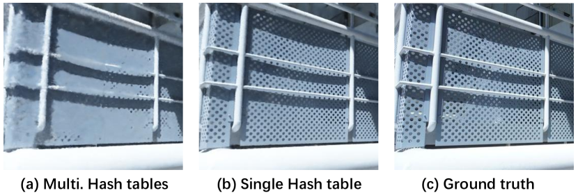
Single v.s. multiple hash tables. We test F²-NeRF on the setting with multiple hash tables, i.e., one hash table for each octree node, with the same budget of parameters as the setting of a single hash table used in the paper. In this setting, the size of each hash table is $L/n_{l}$, where $L=2^{19}$ is the overall table size and $n_{l}$ is the number of leaf octree nodes. Fig. 16 shows that when using multiple hash tables, the quality degrades clearly compared to the setting of using a single hash table with multiple hash functions. The reason is that using a global hash table has more flexibility in allocating the representation capacity to different regions.

Figure 16: Visual comparison between using multiple hash tables (a) and single hash table (b) on the “Sky” case of Free dataset.

Figure 17: Visual comparison between w/o regularization losses (a) and w/ regularization losses (b) on the “Bonsai” case in NeRF-360-V2 dataset.

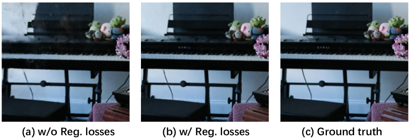
Effect of regularization losses. As shown in Fig. 17, when regularization losses are not used, the foggy artifacts appear and the rendered result is not clear, especially on the regions with pure colors.

Method	Hydrant	Lab	Pillar	Road	Sky	Stair	Grass
NeRF++ [62]	22.21	21.82	25.73	23.29	23.91	26.08	21.26
mip-NeRF-360	25.03	26.57	29.22	27.07	26.99	29.79	24.39
mip-NeRF-360 (short) [3]	21.01	21.17	24.12	21.49	22.29	24.27	19.87
Plenoxels [58]	19.82	18.12	18.74	21.31	18.22	21.41	16.28
DVGO [39]	22.10	23.78	26.22	23.53	24.26	26.65	20.75
Instant-NGP [26]	22.30	23.21	25.88	24.24	25.80	27.79	21.82
F2-NeRF	24.34	25.92	28.76	26.76	26.41	29.19	22.87

Table 10: Scene breakdown on the Free dataset.

Method	Fern	Flower	Fortress	Horns	Leaves	Orchids	Room	Trex
NeRF [25]	25.17	27.40	31.16	27.45	20.92	20.36	32.70	26.80
mip-NeRF [2]	25.12	27.79	31.42	27.55	20.97	20.28	32.52	27.16
Plenoxels [58]	25.46	27.83	31.09	27.58	21.41	20.24	30.22	26.48
TensoRF [6]	25.27	28.60	31.36	28.14	21.30	19.87	32.35	26.97
DVGO [39]	25.08	27.62	30.44	27.59	21.00	20.33	31.53	27.17
Instant-NGP [26]	25.13	27.07	30.96	27.32	12.08	19.80	31.56	26.82
F2-NeRF	25.26	27.48	31.49	27.84	20.68	20.10	32.23	27.26

Table 11: Scene breakdown on the LLFF dataset.

Method	Bicycle	Bonsai	Counter	Garden	Kitchen	Room	Stump
NeRF++ [62]	22.64	29.15	26.38	24.32	27.80	28.87	24.34
mip-NeRF-360 [3]	23.99	33.06	29.51	26.10	32.13	31.53	26.27
Plenoxels [58]	21.39	23.65	25.23	22.71	24.00	26.38	20.08
DVGO [39]	22.12	27.80	25.76	24.34	26.00	28.33	23.59
Instant-NGP [26]	22.08	29.86	26.37	24.26	28.27	28.90	23.93
F2-NeRF	22.11	29.65	25.36	24.76	28.97	29.30	24.60

Table 12: Scene breakdown on the NeRF-360-V2 dataset.

C.5 Per-scene results

We provide the per-scene results on the Free dataset, NeRF-360-V2 dataset, and LLFF dataset in Table 10, Table 12, and Table 11 respectively. The results are reported in the metric of PSNR. Table 9 provides per-scene results on different warping and sampling methods on the Free dataset. We note that the longer the trajectory is (e.g., the “stair” and “grass”), the relatively better performance our perspective warping method with the perspective sampling achieves than the inverse sphere warping method.

Figure 18: Additional visual comparions on the Free dataset.

C.6 More visual results

We provide more visual comparisons on the Free dataset in Fig. 18.

References

- [1] Kara-Ali Aliev, Artem Sevastopolsky, Maria Kolos, Dmitry Ulyanov, and Victor Lempitsky. Neural point-based graphics. In ECCV, 2020.
- [2] Jonathan T. Barron, Ben Mildenhall, Matthew Tancik, Peter Hedman, Ricardo Martin-Brualla, and Pratul P. Srinivasan. Mip-nerf: A multiscale representation for anti-aliasing neural radiance fields. In ICCV, 2021.
- [3] Jonathan T. Barron, Ben Mildenhall, Dor Verbin, Pratul P. Srinivasan, and Peter Hedman. Mip-nerf 360: Unbounded anti-aliased neural radiance fields. In CVPR, 2022.
- [4] Mark Boss, Raphael Braun, Varun Jampani, Jonathan T. Barron, Ce Liu, and Hendrik P. A. Lensch. Nerd: Neural reflectance decomposition from image collections. In ICCV, 2021.
- [5] Chris Buehler, Michael Bosse, Leonard McMillan, Steven J. Gortler, and Michael F. Cohen. Unstructured lumigraph rendering. In SIGGRAPH, 2001.
- [6] Anpei Chen, Zexiang Xu, Andreas Geiger, Jingyi Yu, and Hao Su. Tensorf: Tensorial radiance fields. In ECCV, 2022.
- [7] Anpei Chen, Zexiang Xu, Fuqiang Zhao, Xiaoshuai Zhang, Fanbo Xiang, Jingyi Yu, and Hao Su. Mvsnerf: Fast generalizable radiance field reconstruction from multi-view stereo. In ICCV, 2021.
- [8] Abe Davis, Marc Levoy, and Frédo Durand. Unstructured light fields. Comput. Graph. Forum, 2012.
- [9] Paul E. Debevec, Camillo J. Taylor, and Jitendra Malik. Modeling and rendering architecture from photographs: A hybrid geometry- and image-based approach. In SIGGRAPH, 1996.
- [10] Helisa Dhamo, Keisuke Tateno, Iro Laina, Nassir Navab, and Federico Tombari. Peeking behind objects: Layered depth prediction from a single image. Pattern Recognit. Lett., 2019.
- [11] Rizal Fathony, Anit Kumar Sahu, Devin Willmott, and J Zico Kolter. Multiplicative filter networks. In International Conference on Learning Representations, 2020.
- [12] John Flynn, Michael Broxton, Paul E. Debevec, Matthew DuVall, Graham Fyffe, Ryan S. Overbeck, Noah Snavely, and Richard Tucker. Deepview: View synthesis with learned gradient descent. In CVPR, 2019.
- [13] Steven J. Gortler, Radek Grzeszczuk, Richard Szeliski, and Michael F. Cohen. The lumigraph. In SIGGRAPH, 1996.
- [14] Tong He, John P. Collomosse, Hailin Jin, and Stefano Soatto. Deepvoxels++: Enhancing the fidelity of novel view synthesis from 3d voxel embeddings. In ACCV, 2020.
- [15] Diederik P Kingma and Jimmy Ba. Adam: A method for stochastic optimization. arXiv preprint arXiv:1412.6980, 2014.
- [16] Anat Levin and Frédo Durand. Linear view synthesis using a dimensionality gap light field prior. In CVPR, 2010.
- [17] Zhengqi Li, Wenqi Xian, Abe Davis, and Noah Snavely. Crowdsampling the plenoptic function. In ECCV, 2020.
- [18] David B Lindell, Dave Van Veen, Jeong Joon Park, and Gordon Wetzstein. Bacon: Band-limited coordinate networks for multiscale scene representation. In Proceedings of the IEEE/CVF Conference on Computer Vision and Pattern Recognition, pages 16252–16262, 2022.
- [19] Lingjie Liu, Jiatao Gu, Kyaw Zaw Lin, Tat-Seng Chua, and Christian Theobalt. Neural sparse voxel fields. In NeurIPS, 2020.
- [20] Yuan Liu, Sida Peng, Lingjie Liu, Qianqian Wang, Peng Wang, Christian Theobalt, Xiaowei Zhou, and Wenping Wang. Neural rays for occlusion-aware image-based rendering. arxiv CS.CV 2107.13421, 2021.
- [21] Stephen Lombardi, Tomas Simon, Jason M. Saragih, Gabriel Schwartz, Andreas M. Lehrmann, and Yaser Sheikh. Neural volumes: learning dynamic renderable volumes from images. ACM Trans. Graph., 2019.
- [22] Stephen Lombardi, Tomas Simon, Gabriel Schwartz, Michael Zollhöfer, Yaser Sheikh, and Jason M. Saragih. Mixture of volumetric primitives for efficient neural rendering. ACM Trans. Graph., 2021.
- [23] Julien NP Martel, David B Lindell, Connor Z Lin, Eric R Chan, Marco Monteiro, and Gordon Wetzstein. Acorn: Adaptive coordinate networks for neural scene representation. arXiv preprint arXiv:2105.02788, 2021.
- [24] Ben Mildenhall, Pratul P. Srinivasan, Rodrigo Ortiz Cayon, Nima Khademi Kalantari, Ravi Ramamoorthi, Ren Ng, and Abhishek Kar. Local light field fusion: practical view synthesis with prescriptive sampling guidelines. ACM Trans. Graph., 2019.
- [25] Ben Mildenhall, Pratul P. Srinivasan, Matthew Tancik, Jonathan T. Barron, Ravi Ramamoorthi, and Ren Ng. Nerf: Representing scenes as neural radiance fields for view synthesis. In ECCV, 2020.
- [26] Thomas Müller, Alex Evans, Christoph Schied, and Alexander Keller. Instant neural graphics primitives with a multiresolution hash encoding. ACM Trans. Graph., 2022.
- [27] Jacob Munkberg, Jon Hasselgren, Tianchang Shen, Jun Gao, Wenzheng Chen, Alex Evans, Thomas Müller, and Sanja Fidler. Extracting triangular 3d models, materials, and lighting from images. In CVPR, 2022.
- [28] Michael Oechsle, Songyou Peng, and Andreas Geiger. UNISURF: unifying neural implicit surfaces and radiance fields for multi-view reconstruction. In ICCV, 2021.
- [29] Adam Paszke, Sam Gross, Francisco Massa, Adam Lerer, James Bradbury, Gregory Chanan, Trevor Killeen, Zeming Lin, Natalia Gimelshein, Luca Antiga, et al. Pytorch: An imperative style, high-performance deep learning library. In NeurIPS, 2019.
- [30] Sameera Ramasinghe and Simon Lucey. Beyond periodicity: Towards a unifying framework for activations in coordinate-mlps. In European Conference on Computer Vision, pages 142–158. Springer, 2022.
- [31] Leonid I Rudin and Stanley Osher. Total variation based image restoration with free local constraints. In Proceedings of 1st international conference on image processing, volume 1, pages 31–35. IEEE, 1994.
- [32] Jonathan Shade, Steven J. Gortler, Li-wei He, and Richard Szeliski. Layered depth images. In SIGGRAPH, 1998.
- [33] Meng-Li Shih, Shih-Yang Su, Johannes Kopf, and Jia-Bin Huang. 3d photography using context-aware layered depth inpainting. In CVPR, 2020.
- [34] Vincent Sitzmann, Julien Martel, Alexander Bergman, David Lindell, and Gordon Wetzstein. Implicit neural representations with periodic activation functions. Advances in Neural Information Processing Systems, 33:7462–7473, 2020.
- [35] Vincent Sitzmann, Justus Thies, Felix Heide, Matthias Nießner, Gordon Wetzstein, and Michael Zollhöfer. Deepvoxels: Learning persistent 3d feature embeddings. In CVPR, 2019.
- [36] Vincent Sitzmann, Michael Zollhöfer, and Gordon Wetzstein. Scene representation networks: Continuous 3d-structure-aware neural scene representations. In NeurIPS, 2019.
- [37] Pratul P. Srinivasan, Richard Tucker, Jonathan T. Barron, Ravi Ramamoorthi, Ren Ng, and Noah Snavely. Pushing the boundaries of view extrapolation with multiplane images. In CVPR, 2019.
- [38] Mohammed Suhail, Carlos Esteves, Leonid Sigal, and Ameesh Makadia. Generalizable patch-based neural rendering. arXiv preprint arXiv:2207.10662, 2022.
- [39] Cheng Sun, Min Sun, and Hwann-Tzong Chen. Direct voxel grid optimization: Super-fast convergence for radiance fields reconstruction. In CVPR, 2022.
- [40] Towaki Takikawa, Joey Litalien, Kangxue Yin, Karsten Kreis, Charles Loop, Derek Nowrouzezahrai, Alec Jacobson, Morgan McGuire, and Sanja Fidler. Neural geometric level of detail: Real-time rendering with implicit 3d shapes. In Proceedings of the IEEE/CVF Conference on Computer Vision and Pattern Recognition, pages 11358–11367, 2021.
- [41] Matthew Tancik, Vincent Casser, Xinchen Yan, Sabeek Pradhan, Ben Mildenhall, Pratul P Srinivasan, Jonathan T Barron, and Henrik Kretzschmar. Block-nerf: Scalable large scene neural view synthesis. In CVPR, 2022.
- [42] Matthew Tancik, Ethan Weber, Evonne Ng, Ruilong Li, Brent Yi, Justin Kerr, Terrance Wang, Alexander Kristoffersen, Jake Austin, Kamyar Salahi, Abhik Ahuja, David McAllister, and Angjoo Kanazawa. Nerfstudio: A modular framework for neural radiance field development, 2023.
- [43] Ayush Tewari, Justus Thies, Ben Mildenhall, Pratul Srinivasan, Edgar Tretschk, W Yifan, Christoph Lassner, Vincent Sitzmann, Ricardo Martin-Brualla, Stephen Lombardi, et al. Advances in neural rendering. Computer Graphics Forum, 41(2):703–735, 2022.
- [44] Justus Thies, Michael Zollhöfer, and Matthias Nießner. Deferred neural rendering: image synthesis using neural textures. ACM Trans. Graph., 2019.
- [45] Richard Tucker and Noah Snavely. Single-view view synthesis with multiplane images. In CVPR, 2020.
- [46] Shubham Tulsiani, Richard Tucker, and Noah Snavely. Layer-structured 3d scene inference via view synthesis. In ECCV, 2018.
- [47] Haithem Turki, Deva Ramanan, and Mahadev Satyanarayanan. Mega-nerf: Scalable construction of large-scale nerfs for virtual fly-throughs. In CVPR, 2022.
- [48] Michael Waechter, Nils Moehrle, and Michael Goesele. Let there be color! large-scale texturing of 3d reconstructions. In ECCV, 2014.
- [49] Dan Wang, Xinrui Cui, Septimiu Salcudean, and Z Jane Wang. Generalizable neural radiance fields for novel view synthesis with transformer. arXiv preprint arXiv:2206.05375, 2022.
- [50] Peng Wang, Lingjie Liu, Yuan Liu, Christian Theobalt, Taku Komura, and Wenping Wang. Neus: Learning neural implicit surfaces by volume rendering for multi-view reconstruction. In NeurIPS, 2021.
- [51] Qianqian Wang, Zhicheng Wang, Kyle Genova, Pratul P. Srinivasan, Howard Zhou, Jonathan T. Barron, Ricardo Martin-Brualla, Noah Snavely, and Thomas A. Funkhouser. Ibrnet: Learning multi-view image-based rendering. In CVPR, 2021.
- [52] Svante Wold, Kim Esbensen, and Paul Geladi. Principal component analysis. Chemometrics and intelligent laboratory systems, 2(1-3):37–52, 1987.
- [53] Daniel N. Wood, Daniel I. Azuma, Ken Aldinger, Brian Curless, Tom Duchamp, David Salesin, and Werner Stuetzle. Surface light fields for 3d photography. In SIGGRAPH, 2000.
- [54] Yuanbo Xiangli, Linning Xu, Xingang Pan, Nanxuan Zhao, Anyi Rao, Christian Theobalt, Bo Dai, and Dahua Lin. Bungeenerf: Progressive neural radiance field for extreme multi-scale scene rendering. In ECCV, 2022.
- [55] Qiangeng Xu, Zexiang Xu, Julien Philip, Sai Bi, Zhixin Shu, Kalyan Sunkavalli, and Ulrich Neumann. Point-nerf: Point-based neural radiance fields. In CVPR, 2022.
- [56] Lior Yariv, Jiatao Gu, Yoni Kasten, and Yaron Lipman. Volume rendering of neural implicit surfaces. Advances in Neural Information Processing Systems, 34:4805–4815, 2021.
- [57] Lior Yariv, Yoni Kasten, Dror Moran, Meirav Galun, Matan Atzmon, Basri Ronen, and Yaron Lipman. Multiview neural surface reconstruction by disentangling geometry and appearance. NeurIPS, 2020.
- [58] Alex Yu, Sara Fridovich-Keil, Matthew Tancik, Qinhong Chen, Benjamin Recht, and Angjoo Kanazawa. Plenoxels: Radiance fields without neural networks. In CVPR, 2022.
- [59] Alex Yu, Ruilong Li, Matthew Tancik, Hao Li, Ren Ng, and Angjoo Kanazawa. Plenoctrees for real-time rendering of neural radiance fields. In ICCV, 2021.
- [60] Alex Yu, Vickie Ye, Matthew Tancik, and Angjoo Kanazawa. pixelnerf: Neural radiance fields from one or few images. In CVPR, 2021.
- [61] Kai Zhang, Fujun Luan, Qianqian Wang, Kavita Bala, and Noah Snavely. Physg: Inverse rendering with spherical gaussians for physics-based material editing and relighting. In CVPR, 2021.
- [62] Kai Zhang, Gernot Riegler, Noah Snavely, and Vladlen Koltun. Nerf++: Analyzing and improving neural radiance fields. arxiv CS.CV 2010.07492, 2020.
- [63] Xiuming Zhang, Pratul P. Srinivasan, Boyang Deng, Paul E. Debevec, William T. Freeman, and Jonathan T. Barron. Nerfactor: Neural factorization of shape and reflectance under an unknown illumination. arxiv CS.CV 2106.01970, 2021.
- [64] Tinghui Zhou, Richard Tucker, John Flynn, Graham Fyffe, and Noah Snavely. Stereo magnification: learning view synthesis using multiplane images. ACM Trans. Graph., 2018.