A reinforced learning approach to optimal design under model uncertainty

Abstract

Optimal designs are usually model-dependent and likely to be sub-optimal if the postulated model is not correctly specified. In practice, it is common that a researcher has a list of candidate models at hand and a design has to be found that is efficient for selecting the true model among the competing candidates and is also efficient (optimal, if possible) for estimating the parameters of the true model. In this article, we use a reinforced learning approach to address this problem. We develop a sequential algorithm, which generates a sequence of designs which have asymptotically, as the number of stages increases, the same efficiency for estimating the parameters in the true model as an optimal design if the true model would have correctly been specified in advance. A lower bound is established to quantify the relative efficiency between such a design and an optimal design for the true model in finite stages. Moreover, the resulting designs are also efficient for discriminating between the true model and other rival models from the candidate list. Some connections with other state-of-the-art algorithms for model discrimination and parameter estimation are discussed and the methodology is illustrated by a small simulation study.

Keywords: Model discrimination; Optimal design; Reinforcement learning; Sequential design; Thompson sampling.

1 Introduction

To enhance the statistical efficiency of experiments with limited budgets, optimal design is one of the most commonly used concepts in statistics. Meanwhile, there exists an enormous amount of literature on constructing optimal designs (see, for example, Pukelsheim,, 2006; Atkinson et al.,, 2007; Pronzato and Pázman,, 2013, and the references therein). Most of the existing approaches are model dependent, which means that the statistical relationship between control factors and possible responses is assumed to be known before planning an experiment. Therefore, one can leverage model information to find optimal designs.

In many applications, a model cannot be specified before the experiment and a common approach to address this situation in the construction of designs is to assume that the true model is contained in a class of candidate models. In this case, a good design should be efficient for the identification of the true model and for the estimation of the corresponding parameters. However, it is well known that an optimal design for model discrimination often has a relatively poor performance for parameter estimation (see, for example, Atkinson,, 2008). On the other hand, an optimal design for parameter estimation under a given parametric model usually does not provide enough design points to check its goodness-of-fit, for example by comparing it with a wider candidate model.

Because of the importance to incorporate model uncertainty in the design of experiments, several authors have worked on the problem of constructing efficient designs for competing candidate models and meanwhile there exists a vast amount of literature on this topic. A common approach is to conduct a two-stage (or multi-stage) design where the first stage is tailored for model discrimination, and in the later stages, an optimal design is constructed for the selected model (see, for example, Hill et al.,, 1968; Montepiedra and Yeh,, 1998). Other authors propose designs to optimize compound or constraint optimality criteria that incorporate all candidate models. Typical examples are the maximization average or the minimum of design efficiencies for all candidate models (see Läuter,, 1974; Dette,, 1990; Woods et al.,, 2006, among many others) or the maximization of a criterion for one particular model under the constraint that the efficiencies in all other candidate models exceed certain thresholds (see Cook and Wong,, 1994; Biedermann et al.,, 2009, among others). Alternatively, one may embed the model of interest in a more general model and then find either an optimal design for estimating all parameters in the enlarged model or an optimal design for estimating the parameters in the enlarged model which are not contained in the original model (see Stigler,, 1971; Song and Wong,, 1999). Closely related to this approach are $T$-optimal designs, which are particularly tailored to model discrimination between not necessarily nested models (Atkinson and Fedorov,, 1975; López-Fidalgo et al.,, 2007; Dette and Titoff,, 2009). Moreover, some model-free designs, such as uniform designs, are usually served as another possible solution. In particular, Hickernell and Liu, (2002) demonstrate that uniform designs yield both reasonable efficiencies and robustness and Moon et al., (2012) and Joseph et al., (2015) point out that uniform designs with good projection properties are desirable for factor screening. Finally, one may combine optimality criteria for model discrimination and parameter estimation by a compound or constrained criterion to find a good design for both purposes (see Dette and Franke,, 2000; Atkinson,, 2008; Tommasi,, 2009; López-Fidalgo et al.,, 2007; May and Tommasi,, 2014). Another possibility is to hybrid two types of designs (see, for example Waterhouse et al.,, 2008).

Despite the great success achieved by these methods, they do not yield to an optimal solution, namely a design, which approximates the optimal design for parameter estimation in the true (but before the experiment unknown) model under investigation. In particular, selection uncertainty unavoidably occurs in multi-stage approaches and the resulting designs may be far away from the optimal one. Increasing budgets on model discrimination will mitigate selection inaccuracy, but the resultant designs may still have poor performance since discrimination designs are usually not efficient for parameter estimation. Except for some specific examples, one can not expect that a robust design is also an optimal design for parameter estimation under the true model. Optimal designs for a compound or constraint criterion addressing model discrimination and parameter estimation also suffer from a similar problem.

Our contribution: In this article, we use a reinforced learning approach to construct a sequence of sequential designs, which approximates the optimal design for the true (but unknown) model in the presence of a list of competing candidate models. Our basic idea is to select in each stage an optimal design from the list of optimal designs for the candidate models by Thompson sampling, which has been proved to be optimal in the reinforcement learning framework (see, for example, Auer et al.,, 2002; Agrawal and Goyal,, 2012). The regret required for this approach is defined by design efficiencies, and the posterior distribution is updated by a model selection step in each stage. As our method achieves a minimal regret in design efficiency, we obtain an asymptotically optimal design (for the true model) combining all designs from the different stages. It is proved that the sequence of efficiencies (in the true model) of the resulting designs converge to one, meaning that the designs approximate the optimal design in the true model. In particular, we derive explicit lower bounds for the efficiency of the sequential design after a finite number of stages.

By the reinforced learning approach, we implement a design strategy, which addresses the different statistical objectives at different stages of the experiment and can be regarded as an efficient adaptive hybrid design. The works most similar to ours are Biswas and Chaudhuri, (2002), Tommasi, (2009) and May and Tommasi, (2014), who propose sequential algorithms in model discrimination and parameter estimation for nested linear and non-linear models. Here the key idea is to sequentially adjust the weights in a compound (or hybrid) criterion that incorporates the estimation efficiency in the different candidate models. However, these methods only take the design in the final stage into account and rely heavily on the assumption of nested models. Moreover, both the sequential designs in Biswas and Chaudhuri, (2002) and May and Tommasi, (2014) require that all competing models are estimable using the data from the current stage or all historical data. As a result, the experimenter may spend more costs in model discrimination than is really necessary. The reinforced learning approach avoids these problems and provides an interesting alternative to the commonly used strategies for designing experiments under model uncertainty.

2 Preliminaries

2.1 Problem setups

Consider an experiment, where for a given predictor, say $\bm{x}$, a response $y$ can be observed. For the statistical analysis, it is usually assumed that $y$ is a realization of a random variable $Y$ with a conditional distribution function $F(y|\bm{x})$. Let ${\cal X}$ denote a compact subset of an Euclidean space, then we assume that we can take observations at each $\bm{x}\in{\cal X}$, where observations at different experimental conditions are assumed to be independent. As pointed out in the introduction, a large part of the literature on optimal design assumes a parametric model, say $F(y|\bm{x};\bm{\beta})$ for the distribution of $Y$. Here $F$ is a known conditional distribution and $\bm{\beta}$ is the parameter of interest, which has to be estimated from the data.

In many applications, it is difficult to fix a concrete model before any experiments have been carried out. However, often the experimenter has several candidate models in mind which could fit the data well. To address this problem in the construction of optimal designs, we assume that the “true” model is an element of a set of $\mathrm{K}$ candidate models denoted by $\mathcal{M}=\{M_{1},\ldots,M_{\mathrm{K}}\}$, where the distribution of the $j$th model $M_{j}$ is given by $F_{j}(y|\bm{x};\bm{\beta}_{j})$ and $\bm{\beta}_{j}$ denotes the $p_{j}$-dimensional parameter of interest ($j=1,\ldots,\mathrm{K}$). We emphasize that the design space for the predictor $\bm{x}$ may be different for different models although this is not reflected in our notation. In this work, we aim to find designs that have the highest estimation efficiency under the true model.

We begin with introducing some basic concepts and notations of optimal design theory for a given model, say $M_{j}\in\mathcal{M}$. We define an approximate design as a probability measure with finite support, that is $\xi=\{(\bm{x}_{i},\omega_{i}):i=1,\ldots,m\}$, where $\bm{x}_{1},\ldots,\bm{x}_{m}\in{\cal X}$, $\omega_{1},\ldots,\omega_{m}>0$ and $\sum_{i=1}^{m}\omega_{i}=1$. If $n$ independent observations can be taken to estimate $\bm{\beta}_{j}$, the quantities $n\omega_{i}$ are rounded to integers, say $n_{i}$, such that $\sum_{i=1}^{m}n_{i}=n$, and $n_{i}$ observations are taken at each $\bm{x}_{i}$ ($i=1,\ldots,m$). In this case, under standard assumptions, the asymptotic covariance matrix of the maximum likelihood estimator is given by $n^{-1}I_{j}^{-1}(\xi)$, where $I_{j}(\xi)=\sum_{i=1}^{m}\omega_{i}I_{j}(\bm{x}_{i},\bm{\beta}_{j})$ is the information matrix of the design $\xi$, $I_{j}(\bm{x}_{i},\bm{\beta}_{j})$ denotes the Fisher information matrix at a single design point $\bm{x}_{i}$ (in model $M_{j}$), and we do not reflect a possible dependence of the information matrix $I_{j}(\xi)$ on the parameter $\bm{\beta}_{j}$ in our notation. The model $M_{j}$ (more precisely the parameter $\bm{\beta}_{j}$) is called estimable by the design $\xi$ if the matrix $I_{j}(\xi)$ is non-singular. An optimal design for the model $M_{j}$ maximizes a real-valued function, say $\phi_{j}$ of the information matrix $I_{j}(\xi)$ in the class of all designs. Here $\phi_{j}$ is an information function in the sense of Pukelsheim, (2006), that is a positively homogeneous, concave, non-negative, non-constant, and upper semi-continuous function on the space of non-negative definite matrices. Typical examples include the famous $D$-optimality criterion $\phi_{j}(\xi)=\{\det(I_{j}(\xi))\}^{1/p_{j}}$ and the $A$-optimality criterion $\phi_{j}(\xi)=\{{\rm tr}({p_{j}}^{-1}I_{j}^{-1}(\xi))\}^{-1}$, where $p_{j}$ denotes the dimension of the parameter $\bm{\beta}_{j}$. Throughout this paper we denote a design maximizing $\phi_{j}$ as $\phi_{j}$-optimal design and assume that $\phi_{j}(\xi)=0$ if the information matrix $I_{j}(\xi)$ is singular. This property is satisfied for almost all optimality criteria considered in practice.

In many cases, in particular for non-linear models, the information matrix also depends on the unknown parameter. Following Chernoff, (1953), we use the concept of “locally optimal” design and assume in this case that an initial guess for the unknown parameter $\bm{\beta}_{j}$ is available. Such an approach is reasonable if the locally optimal designs are not too sensitive with respect to the choice of the unknown parameter. A typical example appears in the modeling of dose-response relationships in phase II clinical trials by non-linear regression models, where already some information from phase I is available (see, for example, Bretz et al.,, 2005). In this context, Dette et al., (2008) investigated the robustness of optimal designs for estimating the minimum effective dose from a dose-response curve with respect to the specification of the unknown parameter. Their results suggest that locally optimal designs are moderately robust with respect to a misspecification of the model parameters but highly sensitive with respect to a misspecification of the regression function.

To address this problem in the design of experiments under model uncertainty, we denote the index corresponding to the true model, say $M_{\mathrm{true}}\in\mathcal{M}=\{M_{1},\ldots,M_{\mathrm{K}}\}$, by the subscript “$\mathrm{true}$” in the following discussion. Of course, an optimal design for the true model in the set $\mathcal{M}$ conceptually refers to a design $\xi^{*}$ maximizing $\phi_{\mathrm{true}}(\xi)=\phi_{\mathrm{true}}(I_{\mathrm{true}}(\xi))$. However, a little care is necessary since the optimal design for the true model may not be unique in general, and an optimal design under an incorrect model may also be optimal for the true model as indicated in the following example.

Example 1.

Assume that the class $\mathcal{M}$ consists of three trigonometric regression models

$$Y=\beta_{0}+\sum_{l=1}^{j}\left(\beta_{2l-1}\cos(lt)+\beta_{2l}\sin(lt)\right)+\varepsilon~{},~{}~{}$$

of degree $j=1,2,3$ and that the design space is given by the interval $[0,2\pi)$. It is proved in Section 9.16 of Pukelsheim, (2006) that every uniform design with more than $2j+1$ support points is $\Phi_{q}$-optimal for the trigonometric regression model of degree $j$, which means that the design maximizes the criterion $\Phi_{q}(\xi)=\{{p_{j}}^{-1}{\rm tr}(I_{j}^{q}(\xi))\}^{1/q}$, where $q\in[-\infty,1)$. Note that the cases $q=0$, $q=-1$, and $q=-\infty$ correspond to widely used $D$-, $A$- and $E$-optimality criterion, respectively. Consequently, a uniform design with seven equispaced support points is optimal for all three models. However, when $M_{1}$ or $M_{2}$ is the true model, one can also construct a design with less than seven supports to achieve the same efficiency. In this case, an experimenter would prefer this design since it further reduces the cost of altering the experimental settings.

In the following, we formally define an optimal design for the true model among the competing candidate models from the set $\mathcal{M}$.

Definition 1.

A design $\xi^{*}$ is said to be $\mathcal{M}$-optimal, if and only if $\xi$ maximizes the functional

$$\phi_{\mathrm{true}}(\xi)\gamma_{\xi},$$ (2.1)

where $\gamma_{\xi}$ is an indicator, which is one if and only if the number of support points of $\xi$ is minimal among all $\phi_{\mathrm{true}}$-optimal designs for the true model.

Note that the true model can not be estimated by the design under consideration if the corresponding Fisher information matrix $I_{\mathrm{true}}(\xi)$ is singular. In this case, the criterion value is zero (because the criteria vanish for singular matrices, by assumption). Therefore, maximizing the criterion in (2.1) will always result in a design that can be used to estimate all parameters in the true model. On the other hand, a design constructed for a more complicated model is not necessarily a good solution, since a more complex model usually involves more support points. In this scenario, statistical efficiency is not the only standard, the economic costs caused by taking observations at more different experimental conditions should also be taken into account. In general $\phi_{\mathrm{true}}(\xi)\gamma_{\xi}$ will not be maximal unless the design $\xi$ is $\phi_{\mathrm{true}}$-optimal under the true model $M_{\mathrm{true}}$ with a minimal number of support points.

It is worth mentioning that constructing an optimal design with a minimal number of support points is not an easy task. In practice, this condition can be relaxed by the optimal design with a minimal number of support points among optimal designs for the candidate models. For the sake of a simple notation, all optimal designs in this paper refer to the optimal designs for the corresponding models with a minimal number of support points.

2.2 Multi-stage designs

One can not expect to obtain an $\mathcal{M}$-optimal design when the experiment can only be carried out in one stage without enough prior knowledge. In the following, we introduce multi-stage (approximate) designs which is one of the key ingredients in finding an $\mathcal{M}$-optimal design.

In the multi-stage design context, $n_{t}$ observations are taken according to an approximate design $\xi_{(t)}$ at each stage $t$ for $t\in\{1,\ldots,T\}$, where $T$ denotes the total number of possible stages. Let $n:=\sum_{t=1}^{T}{n_{t}}$ be the total sample size. We are interested in finding an $\mathcal{M}$-optimal multi-stage design, that is a sequence of designs $\xi_{(1)},\ldots,\xi_{(T)}$ such that the convex combination $\xi_{\mathcal{M},T}=\sum_{t=1}^{T}(n_{t}/n)\xi_{(t)}$ is in some sense “close” to an $\mathcal{M}$-optimal design. For this purpose we define a corresponding gain of conducting $\xi_{(t)}$ at stage $t$ by

$$r(\xi_{(t)})=\phi_{\mathrm{true}}(\xi_{(t)})\gamma_{\xi_{(t)}},$$ (2.2)

where $\gamma_{\xi_{(t)}}$ is defined in Definition 1. Our approach is then based on finding a sequence of designs $\xi_{(1)},\ldots,\xi_{(T)}$ that achieves the maximum gain at each stage $t$. One possible solution to reach this goal is to select a design from the locally $\phi_{1},\ldots,\phi_{K}$-optimal designs $\xi_{1}^{*},\ldots,\xi_{\mathrm{K}}^{*}$ for the models $M_{1},\ldots,M_{\mathrm{K}}$, respectively. Clearly, if one can select the design $\xi_{\mathrm{true}}^{*}$ infinitely often, such that ${\#\{t|\xi_{(t)}\not=\xi_{\mathrm{true}}^{*}\}}/T$ converges to $0$ as $T\to\infty$ and the sample sizes $n_{t}$ at each stage are of the same order, then an asymptotically $\mathcal{M}$-optimal design can be constructed by aggregating these designs. By this approach, we simplify the problem to a discrete choice problem. Finding a maximum gain design in each stage could then serve as a proxy for finding an $\mathcal{M}$-optimal design.

3 Sequential designs by reinforced learning

To achieve a maximum gain in each stage, the researchers have to appropriately balance two objectives: (a) exploiting the most promising model in the current stage and finding an optimal design to further improve its parameter estimation; (b) exploring an alternative model that may turn out to be the true model in the future and performing an optimal design for it.

Borrowing ideas from reinforcement learning, we will to use multi-armed bandits’ strategies to achieve the balance between exploitation and exploration. To be precise, one can treat the $\mathrm{K}$ candidate designs as arms. One may conduct a batch of experiments sequentially trying out various arms (or candidate designs in our setting) and collect gains to prioritize a design that is good for the true model. Identifying the arm with the highest expected gain and pulling this arm (i.e., conducting experiments according to the corresponding optimal design) infinitely often could then serve as a natural solution for constructing a design which is approximating an $\mathcal{M}$-optimal design.

As pointed out in Agrawal and Goyal, (2013), Thompson’s sampling strategy (Thompson,, 1933) is a Bayesian heuristic reinforcement learning algorithm that can achieve a nearly optimal solution for the dilemma between exploitation and exploration. In the following, we will link the Thompson sampling strategy to the multi-stage $\mathcal{M}$-optimal design. Similar to traditional Thompson sampling, the proposed algorithm for searching a multi-stage $\mathcal{M}$-optimal design alternates among the selection, evaluation, and updating.

We start with some necessary notations. Denote the observations at the stage $t$ according to a design $\xi_{({t})}$ by

$${\cal D}_{t}:=\{(\bm{x}_{n_{0}+\ldots+n_{t-1}+1},Y_{n_{0}+\ldots+n_{t-1}+1}),\ldots,(\bm{x}_{n_{0}+\ldots+n_{t}},Y_{n_{0}+\ldots+n_{t}})\}$$ (3.1)

and define $\zeta_{j}(t)\in\{0,1\}$ as an indicator whether the model $M_{j}$ is chosen as the true model using the data ${\cal D}_{t}$. It is worth mentioning that $\zeta_{j}(t)$ is a random variable. Through the lens of Bayesian model checking and selection techniques, we can further define the posterior probability

$$\theta_{j}(\xi_{({t})}):=\mathbb{P}(\zeta_{j}(t)=1|{\cal D}_{t})$$ (3.2)

that $M_{j}$ is the true model conditional on the data ${\cal D}_{t}$. For mathematical rigor, we only define $\theta_{j}(\xi_{(t)})$ for the models which are estimable. As in traditional Thompson Sampling, the $t$th stage starts off by sampling $\eta_{j}(t)\sim\mathrm{Beta}(a_{j}(t),b_{j}(t))$ from a posterior distribution that serves as a surrogate for $\theta_{j}(\xi_{(t)})$. To be precise, $a_{j}(t)-1$ and $b_{j}(t)-1$ are the numbers of times that model $M_{j}$ is treated as the true model (success) and the improper model (failure) in the first $t-1$ stages, respectively ($j=1,\ldots,\mathrm{K}$). Then, following the Thompson sampling policy we select the index $\tau_{t}\in\{1,\ldots,\mathrm{K}\}$ corresponding to the highest value among $\eta_{1}(t),\ldots,\eta_{\mathrm{K}}(t)$ at stage $t$ and denote by $\xi_{\tau_{t}}^{*}$ the corresponding optimal design. For the first stage, we simply put $a_{j}(1)=b_{j}(1)=1$ for all candidate models opportunities to be selected as the true model at the beginning.

Then in the evaluation step, the user will evaluate all models in the candidate pool and score them using a sample of observations from the design $\xi_{\tau_{t}}^{*}$. However, some care is necessary here, as there might exist models which are not estimable by the design $\xi_{\tau_{t}}^{*}$. To address this problem we conduct some additional experiments at stage $t$ according to a uniform design. More precisely, in each stage $t$, we take $n_{t}$ observations according to a hybrid design $\rho_{t}\xi_{\tau_{t}}^{*}+(1-\rho_{t})\xi_{\rm unif}$, where $\xi_{\rm unif}$ denotes a uniform design and $\rho_{t}\in(0,1)$ denotes the proportion of observations taken according to the optimal design at stage $t$. We use the uniform design here since it has desirable maximin properties with respect to goodness-of-fit testing (Wiens,, 2009). Other discrimination designs can also be applied here as well. We will allow the proportion $\rho_{t}$ to change with $t$, since as the observations began to accumulate we have more confidence in the optimal design we selected. A possible specification of $\rho_{t}$ is $N_{\tau_{t}}(t)/(N_{\tau_{t}}(t)+1)$, where $N_{j}(t)$ denotes the number of times that design $\xi_{j}^{*}$ was chosen until stage $t$. Because all models are estimable by this design we can use a model selection criterion to select the “best” model, say $M_{\psi_{t}}$, among the candidates. In the following we will work with the Bayesian information criterion (BIC, see Schwarz,, 1978), but other model selection techniques including goodness-of-fit tests could be considered as well. Finally, we assign a score $\zeta_{\psi_{t}}(t)=1$ for the selected model and the score $\zeta_{j}{(t)}=0$ for $j\neq{\psi_{t}}$.

The algorithm concludes with an updating step for the beta posterior distribution, setting $a_{j}(t+1)=a_{j}(t)+\zeta_{j}(t)$ and $b_{j}(t+1)=b_{j}(t)+(1-\zeta_{j}(t))$. The details are summarized in Algorithm 1.

Initialize $n_{0}:=0$ and $a_{j}(1)=1$ and $b_{j}(1)=1$ for each arm $j=1,\ldots,\mathrm{K}$.

for $t=1,\ldots,T-1$ do

      

(1) Selection Step

• Generate random variables $\eta_{j}(t)\sim\mathrm{Beta}(a_{j}(t),b_{j}(t))$ for $j=1,\ldots,\mathrm{K}$.

• Choose the one with the largest value among $\{\eta_{j}(t)\}_{j=1}^{\mathrm{K}}$ and denote its index by $\tau_{t}$.

•  

  Take $n_{t}$ observations ${\cal D}_{t}$ defined in (3.1) according to $\xi_{(t)}^{\rm hyb}:=\rho_{t}\xi^{*}_{\tau_{t}}+(1-\rho_{t})\xi_{\rm unif}$,

       where $\xi^{*}_{\tau_{t}}$ is the (locally) optimal design for model $M_{\tau_{t}}$, and $\xi_{\rm unif}$ is a uniform design.

      (2) Evaluation Step

      

• Use the data ${\cal D}_{t}$ and the BIC criterion to select a model in $\mathcal{M}$, and denote the corresponding index by $\psi_{t}$.

• $\zeta_{j}(t)=1$ (true model) if $j=\psi_{t}$ and $\zeta_{j}(t)=0$ if $j\not=\psi_{t}$.

      (3) Updating Step

• Set $a_{j}(t+1)=a_{j}(t)+\zeta_{j}(t)$ and $b_{j}(t+1)=b_{j}(t)+(1-\zeta_{j}(t))$.

Output: The design ($n:=\sum_{t=1}^{T}{n_{t}}$)

$$\textstyle{\xi_{\mathcal{M},T}:=\sum\limits_{t=1}^{T}\frac{n_{t}}{n}\xi_{(t)}^{\rm hyb}=\sum\limits_{t=1}^{T}\frac{n_{t}}{n}\left\{\rho_{t}\xi^{*}_{\tau_{t}}+(1-\rho_{t}){\xi_{\rm unif}}\right\}.}$$ (3.3)

Algorithm 1 Multi-stage $\mathcal{M}$-Optimal Design Algorithm

Remark 1.

Constructing an optimal design in the selection step is not an easy task and in many cases these designs have to be found numerically. Fortunately, many efficient numerical algorithms have been developed for generating optimal designs in different models with respect to different criteria (see, for example, Yu,, 2010; Yang et al.,, 2013; Harman and Lenka,, 2019, for some recent references). Thus, we do not specify a detailed algorithm here for the selection step. After obtaining an approximate optimal design, users may apply a rounding procedure (Pukelsheim,, 2006) to decide about the number of replications at each design point. Alternatively, the exact optimal design algorithm based on mixed-integer second-order cone programming proposed by Sagnol and Harman, (2015) can also be applied.

Remark 2.

To reduce the costs, we can first conduct $n_{\rm test}$ experiments at the beginning. Then we use these $n_{\rm test}$ observations together with $n_{t}-n_{\rm test}$ observations according to the optimal design $\xi_{\tau_{t}}^{*}$ at each stage $t$ to select the best model. Note that conditional on these $n_{\rm test}$ experimental units, the selection results are still independent thus the effects of choosing improper designs will also not be propagated over time.

Remark 3.

In some cases (for example, if the sample size $n_{t}$ is too small) not all models in the class $\mathcal{M}$ may be estimable using observations according to the hybrid design $\xi_{(t)}^{\rm hyb}:=\rho_{t}\xi_{\tau_{t}}^{*}+(1-\rho_{t})\xi_{\rm unif}$ (or by the design in Remark 2). In such a scenario, we propose to modify the operation at stage $t$ as follows. We skip the updating step (3) for the models which are not estimable, say $M_{j}$, and keep $a_{j}(t+1)=a_{j}(t),b_{j}(t+1)=b_{j}(t)$. Consequently, we still have chance to explore such models at the stage $t+1$ due to the relatively large variance of the $\mathrm{Beta}(a_{j}(t+1),b_{j}(t+1))$ distribution. For all estimable models, we adopt a goodness-of-fit test (see, for example Dette,, 1999) and assign $\zeta_{j}(t)=0$ to all models which are rejected. Among the models that cannot be reject by the goodness-of-fit test, we select a model by BIC and define $\zeta_{\psi_{t}}(t)=1$ for the selected model and $\zeta_{j}(t)=0$ for the rest. Note that this procedure will assign $\zeta_{\psi_{t}}(t)=0$ to all models of $\mathcal{M}$ if the goodness-of-fit test rejects all models.

Remark 4.

Compared with searching compound or constrained optimal designs our method offers a computational advantage since we do not need to search for designs for various values of weights or constraints in the criteria. This is a considerable benefit when the multi-objective design is hard to obtain.

Remark 5.

Unlike most sequential designs such as Biswas and Chaudhuri, (2002), which use all observations from previous stages to conduct the model evaluation, Algorithm 1 only uses the data $\mathcal{D}_{t}$ from stage $t$. As a consequence, the algorithm has some ability for exploration and the effects of choosing improper designs will not be propagated over time.

Remark 6.

From the evaluation step and updating step in Algorithm 1, one can clearly see the difference to the single-armed bandit problem. In the evaluation step, we propose to evaluate as many models as possible to make full use of the information from an experiment. Thus, sometimes it can be more efficient than the single-armed bandit in the sense of data exploration. More importantly, such an evaluation method can help the researcher to efficiently identify the true model from the candidates that are well-fitted (or overfitted) with the observed data.

4 Theoretical results

In this section, we investigate some theoretical properties of the proposed algorithm. In particular, two fundamental questions regarding Algorithm 1 will be answered. First, can the true model be correctly identified by the proposed design? Second, how well approximates the design $\xi_{\mathcal{M},T}$ obtained by Algorithm 1 the optimal design $\xi^{*}_{\mathrm{true}}$ in terms of design efficiency? For the sake of a simple notation, we assume throughout this section that the number of runs in all stages is the same, i.e. $n_{1}=\ldots=n_{T}.$

4.1 Asymptotic properties

By Definition 1, the resulting design $\xi_{\mathcal{M},T}$ in (3.3) approximates the $\mathcal{M}$-optimal design $\xi_{\mathcal{M}}$ if one chooses $\xi^{*}_{\mathrm{true}}$ infinitely often in the selection step of Algorithm 1 such that $\#\{t|\xi_{\tau_{t}}\not=\xi^{*}_{\mathrm{true}}\}/T\to 0$. If this happens, the answers to the above two questions are straightforward. In fact, we will show below that the proposed method selects a wrong design only $O(\log(T))$ times - see Lemma 3 in the supplement, for more details. For notational simplicity, we assume $\rho_{t}=N_{\tau_{t}}(t)/(N_{\tau_{t}}(t)+1)$ as suggested in Section 3. Before we present the main results we will impose a mild condition on the selection criterion used in the evaluation step (which is in our case the BIC procedure).

Condition 1.

There exists two constants $\alpha\in(0,1/2)$ and $c\in(\alpha,1-\alpha)$, such that any design $(1-\rho)\xi_{l}^{*}+\rho\xi_{\rm unif}$ with $\rho\in{\cal R}:=\{1/2,2/3,3/4,\ldots\}$ and $l\in\{1,\ldots,\mathrm{K}\}$ satisfies

$$\theta_{\mathrm{true}}(\rho\xi_{l}^{*}+(1-\rho)\xi_{\rm unif})>c+\alpha,$$ (4.1)

and

$$\theta_{j}(\rho\xi_{l}^{*}+(1-\rho)\xi_{\rm unif})<c-\alpha,$$ (4.2)

for any $j\neq\mathrm{true}$.

Condition 1 essentially requires that the decision (or the selection) is stable according to different kinds of designs. Note that the BIC enjoys the selection consistency property (see, for example Claeskens and Hjort,, 2008) and with probability converging to one, this method is able to select the true model from the candidate models. Thus one can expect that Condition 1 holds when $n_{t}$ is not too small. In this case we can show that the design obtained by Algorithm 1 approximates the $\mathcal{M}$-optimal design since the event $\{M_{\tau_{t}}\not=M_{\mathrm{true}}\}$ occurs only finitely many times as $T\to\infty$. Our first result makes this statement precise. Note that by definition the index $\tau_{t}$ is a random variable and consequently the resulting design $\xi_{\mathcal{M},T}$ in Algorithm 1 and its efficiencies are random objects as well.

Theorem 1.

Assume that Condition 1 holds. Then, as $T\to\infty$,

$$\phi_{\mathrm{true}}(\xi_{\mathcal{M},T})\to\phi_{\mathrm{true}}(\xi_{\mathrm{true}}^{*})$$ (4.3)

in probability, where $\xi_{\mathcal{M},T}$ is the design obtained by Algorithm 1, and $\xi_{\mathrm{true}}^{*}$ is the (locally) optimal design for the true model.

Note that Condition 1 is an assumption on the model selection procedure and Theorem 1 holds for any procedure that identifies the true model with high probability. The BIC in Algorithm 1 is one option and one can use other techniques as well to score the candidate models.

Recall the notation of $N_{j}(t)$ as the number of stages where $\xi_{j}^{*}$ is chosen to construct the hybrid design in the selection step of Algorithm 1 until time $t$. When the algorithm stops at time $T$, we propose to finally choose model $M_{j}$ such that $N_{j}(T)$ is the maximum number among $\{N_{1}(T),\ldots,N_{\mathrm{K}}(T)\}$. Our next result yields, as a by-product, the selection consistency of this method.

Theorem 2.

If Condition 1 holds, then the expected number of times that the event $\mathcal{A}(t)=\{M_{\tau_{t}}\neq M_{\mathrm{true}}\}$ happens satisfies

$$\mathbb{E}\Big{[}\sum_{t=1}^{T}\mathbb{I}\left(\mathcal{A}(t)\right)\Big{]}\leq\mathrm{K}\left(2+\frac{2}{\alpha^{2}}\right)+\frac{8\log(T)}{\alpha^{2}}.$$

In particular, as $T\to\infty$, with probability approaching one,

$$N_{\mathrm{true}}(T)=\max\big{\{}N_{1}(T),\ldots,N_{\mathrm{K}}(T)\big{\}}~{}.$$

4.2 Finite stage analysis

In many applications experimental units are expensive, and the number of stages may be limited when users have to take costs into account. In the following, we will take a closer look at the potential loss when the number of different stages has to be restricted. For this purpose we denote by $\xi_{\mathrm{true}}^{*}$ the optimal design for the true model and define

$$\mathrm{Eff}_{\mathrm{true}}(\xi)=\frac{\phi_{\mathrm{true}}(\xi)}{\phi_{\mathrm{true}}(\xi_{\mathrm{true}}^{*})}\in[0,1]$$

as the $\phi_{\mathrm{true}}$-efficiency of a design $\xi$. The following result gives a lower bound for the expectation of this random variable.

Theorem 3.

Assume that Condition 1 holds and that all models in ${\cal M}$ are estimable by $\xi_{(t)}^{\rm hyb}(t=1,\ldots,T)$, then

$$\mathbb{E}\big{[}\mathrm{Eff}_{\mathrm{true}}(\xi_{\mathcal{M},T})\big{]}\geq 1-\frac{(8+\alpha^{2})\log(T)}{\alpha^{2}T}-\frac{\left(2+{2}/{\alpha^{2}}\right)\mathrm{K}}{T}.$$ (4.4)

In the following, we provide an analogous result to Theorem 3 when the Algorithm 1 is modified as proposed in Remark 3. For this statement, we require a slightly stronger assumption than Condition 1.

Condition 2.

If the true model is estimable by the design $\xi_{(t)}^{\rm hyb}$ at stage $t$, then there exists two constants $\alpha\in(0,1/2)$ and $c\in(\alpha,1-\alpha)$, such that any design $(1-\rho)\xi_{l}^{*}+\rho\xi_{\rm unif}$ with $\rho\in{\cal R}:=\{1/2,2/3,3/4,\ldots\}$ and $l\in\{1,\ldots,\mathrm{K}\}$ satisfies

$$\theta_{\mathrm{true}}(\rho\xi_{l}^{*}+(1-\rho)\xi_{\rm unif})>c+\alpha,$$

and

$$\theta_{j}(\rho\xi_{l}^{*}+(1-\rho)\xi_{\rm unif})<c-\alpha,$$

for any $j\neq\mathrm{true}$. Otherwise, for any estimable model $M_{j}$, it holds that

$$\theta_{j}(\rho\xi_{l}^{*}+(1-\rho)\xi_{\rm unif})<c-\alpha.$$

Equipped with Condition 2, we are ready to provide a lower bound of $\mathbb{E}[\mathrm{Eff}_{\mathrm{true}}(\xi_{\mathcal{M},T})]$, which also directly implies the analogous result of Theorem 1 for the modification of Algorithm 1 according to Remark 3.

Theorem 4.

Assume that Condition 2 holds for all $t\in\{1,\ldots,T\}$. If the design $\xi_{\mathcal{M},T}$ is calculated by the modification of Algorithm 1 as proposed in Remark 3, then

$$\mathbb{E}\big{[}\mathrm{Eff}_{\mathrm{true}}(\xi_{\mathcal{M},T})\big{]}\geq 1-\frac{(8\mathrm{K}-8+\alpha^{2})\log(T)}{\alpha^{2}T}-\frac{\left(3+{4}/{\alpha^{2}}\right)\mathrm{K}}{T}-\frac{1}{T}.$$ (4.5)

Remark 7.

It is interesting to see that the risk bound in Theorem 4 is smaller compared with the bound in Theorem 3, especially for a large $\mathrm{K}$. This is the price we have pay for the cases where one cannot explore all candidate models simultaneously.

As shown in Lai and Robbins, (1985), the term $\log(T)$ is the leading order term in the lower bound for any multi-armed bandit algorithm. This can be regarded as a necessary price we pay for model exploration. Roughly speaking, in our algorithm the random variables $\eta_{j}(t)$ may not be concentrated around the mode of the $\mathrm{Beta}(a_{j}(t),b_{j}(t))$ distribution when $a_{j}(t)+b_{j}(t)$ is much smaller than $O(\log(T))$.

5 Numerical studies

In this section we study the finite sample properties of the proposed method through several examples.

5.1 Nonlinear models for dose-response studies

In our first example we consider the following three non-linear models which are widely adopted in the dose-response experiments. The three candidates are the Emax, linear and exponential model defined by

$$\begin{split}M_{1}:&~{}~{}Y=f_{1}(d,\bm{\beta}_{1})+\varepsilon:=\beta_{0}+\beta_{1}\frac{d}{d+\beta_{2}}+\varepsilon,\\ M_{2}:&~{}~{}Y=f_{2}(d,\bm{\beta}_{2})+\varepsilon:=\beta_{0}+\beta_{1}d+\varepsilon,\\ M_{3}:&~{}~{}Y=f_{3}(d,\bm{\beta}_{3})+\varepsilon:=\beta_{0}+\beta_{1}\exp(d/\beta_{2})+\varepsilon,\end{split}$$ (5.1)

respectively, where we assume that the error is standard normal distributed. Following the setting in Section 10.5.3 of Pinheiro et al., (2006), the dose $d$ varies in the interval $[0,1]$ and the noise is normal distributed with standard deviation $\sigma=0.65$. The vector of parameters is given by $\bm{\beta}_{1}=(0.2,0.7\delta,0.2)^{\top}$, $\bm{\beta}_{2}=(0.2,0.6\delta)^{\top}$ and $\bm{\beta}_{3}=(0,0.2,1/\log(1+3\delta))^{\top}$, for model $M_{1}$, $M_{2}$ and $M_{3}$, respectively. Here the parameter $\delta$ is used to control the signal-to-noise ratio (SNR) ${\rm var}(\mathbb{E}(Y|d))/\sigma^{2}$. Note that $d_{\infty}:=\min_{i\neq j}\sup_{d}|f_{i}(d,\bm{\beta}_{i})-f_{j}(d,\bm{\beta}_{j})|$ is given by $0.5$ and $0.9$ for $\delta=3$ and $\delta=5$, respectively. We set that total sample size to be $n=150$.

In this example, we investigate the $D$-optimality criterion, that is $\phi_{j}(\xi)=\big{(}\det(I_{j}(\xi))\big{)}^{1/p_{j}}$. Consequently, the $D$-efficiency of a design for the true model is given by

$$\mathrm{Eff}_{\mathrm{true}}^{D}(\xi)=\Big{(}\frac{\det(I_{\mathrm{true}}(\xi))}{\det(I_{\mathrm{true}}(\xi_{\mathrm{true}}^{*}))}\Big{)}^{1/p_{\mathrm{true}}}~{},$$ (5.2)

where $p_{\mathrm{true}}$ is the dimension of the vector of parameters for the true model. The locally $D$-optimal designs for the Emax ($M_{1}$) and exponential model ($M_{3}$) have been determined explicitly in Dette et al., (2010). They are uniform designs supported $d=0$ and $d=1$ and a third point in the interval $(0,1)$, which depends on the model under consideration. These authors also demonstrated that a design for a given model has often low $D$-efficiency for another model. The optimal design for the linear model ($M_{2}$) is is supported at $0$ and $1$ with equal weights .

We apply Algorithm 1 with $T={10}$ stages and sample size $n_{t}=15$ for $t=1,\ldots,{10}$ to conduct a sequential design. Additionally, a “standard design” adopted in Pinheiro et al., (2006) with equal weights at the points $\{0,0.05,0.2,0.6,1\}$, a uniform design with five support points, a compound design maximizing $\{\mathrm{Eff}_{M_{1}}^{D}(\xi)\mathrm{Eff}_{M_{2}}^{D}(\xi)\mathrm{Eff}_{M_{3}}^{D}(\xi)\}^{1/3}$ and a hybrid optimal design defined by $\sum_{k=1}^{3}3^{-1}\xi_{k}^{*}$ are considered for the sake comparison. These designs can be found in Section B of online supplement. Besides the efficiency, the designs are evaluated by their selection accuracy (ACC), which is defined as the probability that the true model is selected using the BIC for model selection based on the final $150$ observations (which are obtained by the different designs). The efficiency and selection accuracy are estimated by $500$ simulation runs. In each simulation we use the $150$ observations obtained by Algorithm 1 for model selection and parameter estimation. For the other designs considered in our study we simply take $150$ new observations at each replication according to the design under consideration.

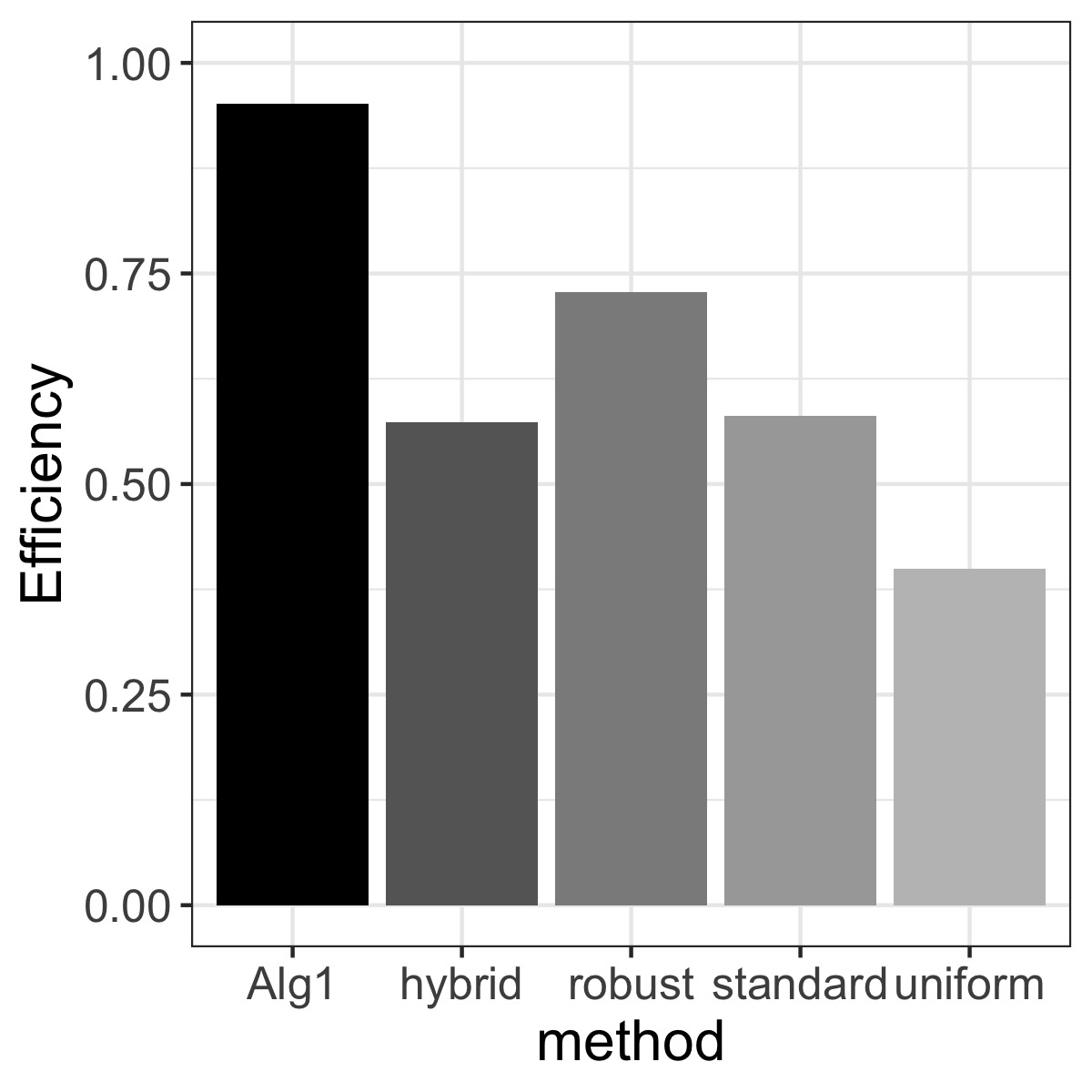
(a) $M_{1}$

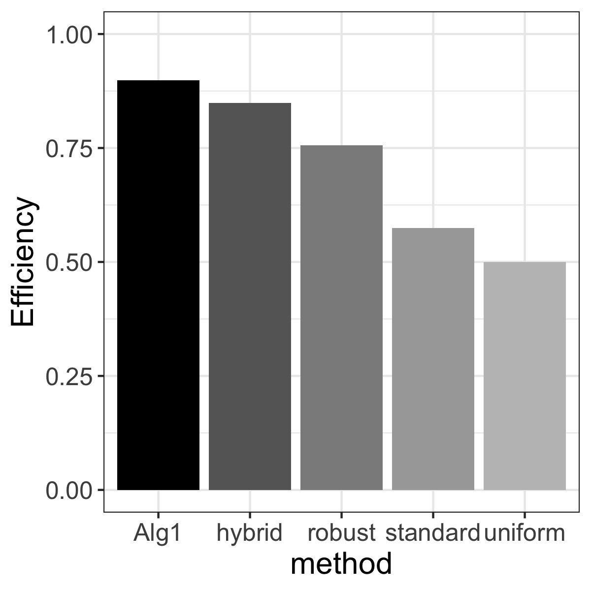
(b) $M_{2}$

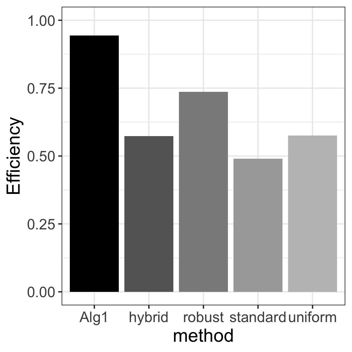
(c) $M_{3}$

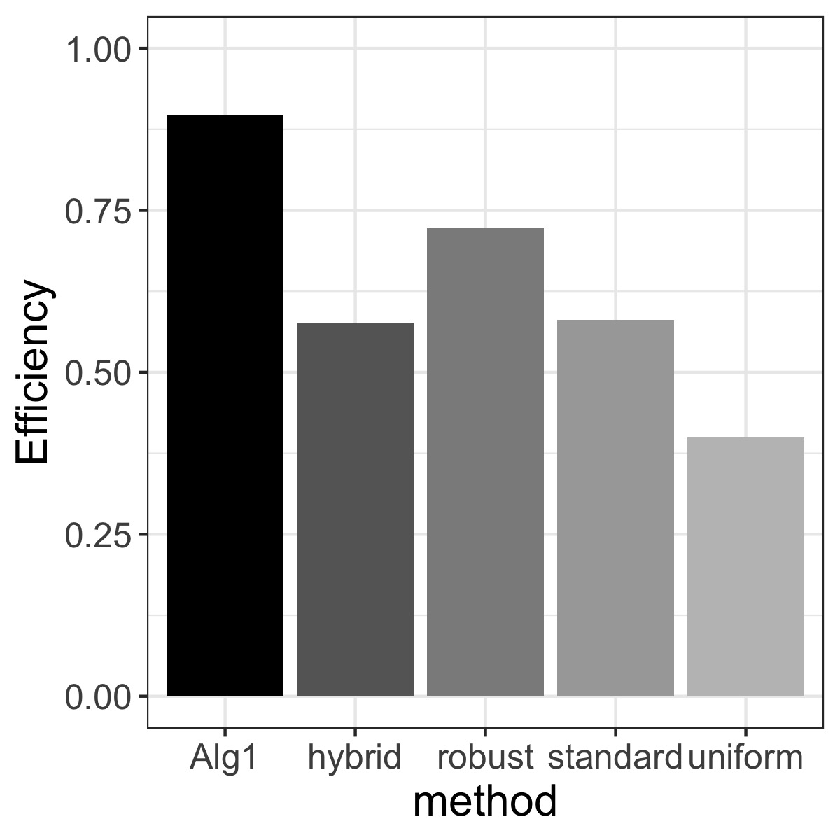
(d) $M_{1}$

(e) $M_{2}$

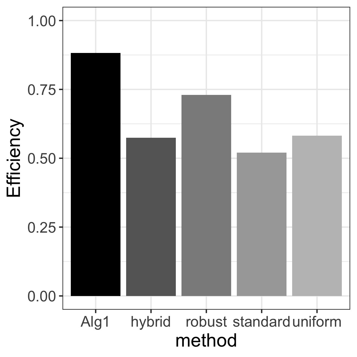
(f) $M_{3}$

Figure 1: $D$-efficiencies defined in (5.2) of different designs under different true models defined in (5.1). Upper part: SNR=3.75; lower part: SNR=1.35.

The $D$-efficiencies are displayed in Figure 1. We observe that for the SNR of $3.75$ the efficiencies of the design $\xi_{\mathcal{M}.T}$ calculated by Algorithm 1 are close to $1$ in all cases under consideration. On the other hand, for a SNR of $1.35$, the $D$-efficiency of the sequential designs are a little smaller. Note that in this case it is harder to distinguish the dose-response curves among the three models based on $15$ observations, which implies a smallr value of $\alpha$ in Condition 1. Thus the numerical results for both scenarios confirm our theoretical findings in Theorem 1 and 3. Moreover, in all cases under consideration the $D$-efficiencies of the proposed sequential designs are larger than the efficiencies of the other competing designs under consideration.

In Figure 2, we investigate the relation between the $D$-efficiency and total sample size $n$ in case, where $M_{1},M_{2}$, and $M_{3}$ is the true model and the SNR is either $1.35$ or $3.75$. We observe that the $D$-efficiencies quickly increase to $1$ when the number of stages increases. We observe that for a SNR of $1.35$ the $D$-efficiencies of the sequential designs obtained by Algorithm 1 are a little smaller than for $3.75$. The difference difference is mostly visible for model $M_{3}$. It can be explained by the fact that in this case the linear and the exponential model are very similar and therefore the BIC tends to select a simpler model instead of the true model.

(a) $M_{1}$

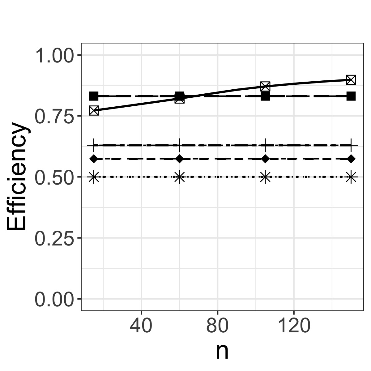
(b) $M_{2}$

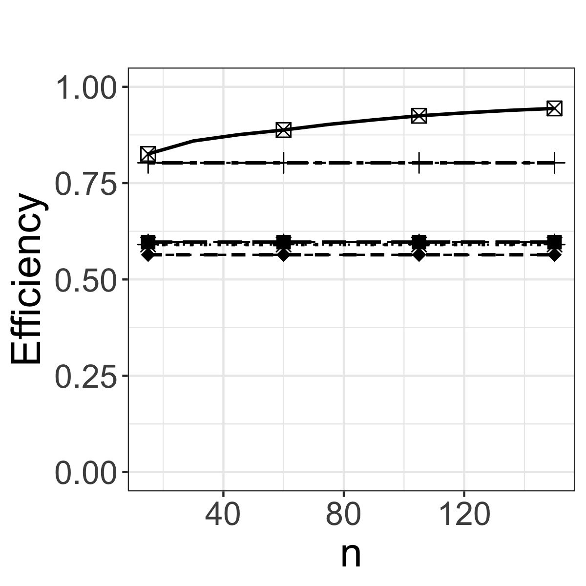
(c) $M_{3}$

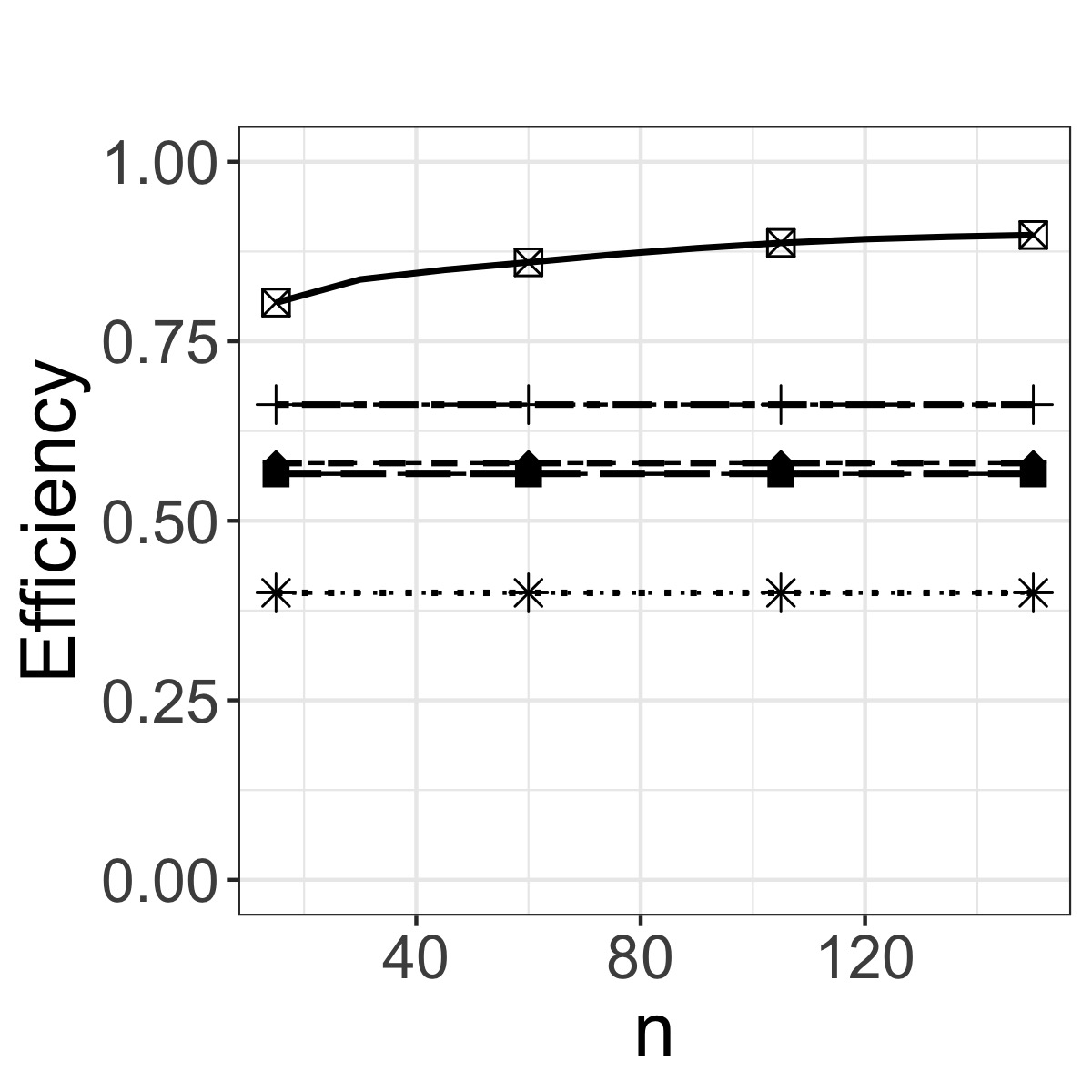
(d) $M_{1}$

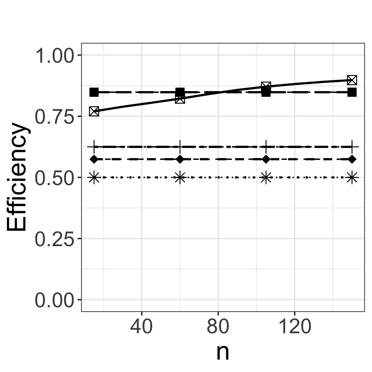
(e) $M_{2}$

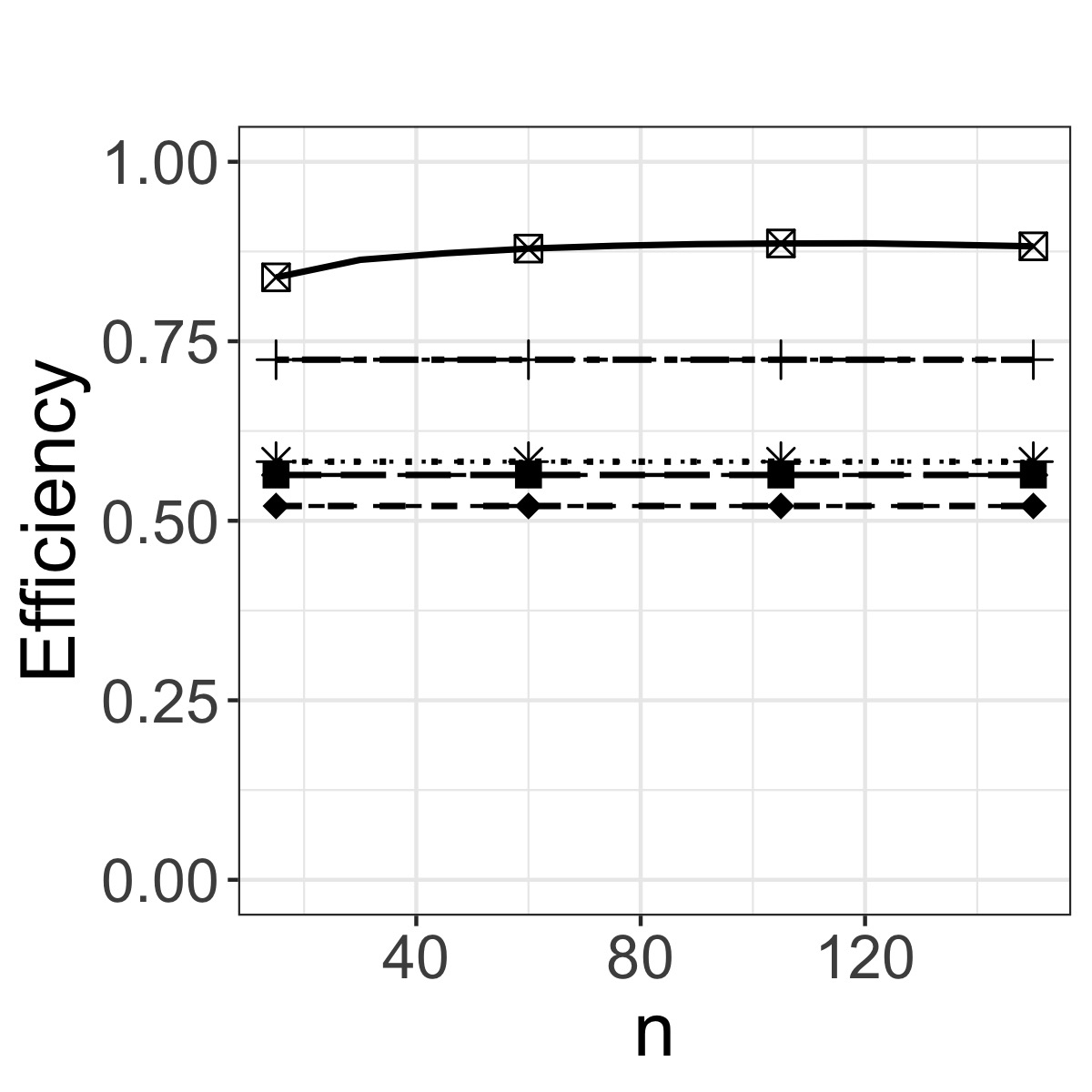
(f) $M_{3}$

Figure 2: $D$-efficiencies (5.2) for the true model as the the total sample size $n$ of the sequential design is increasing. The models are given by (5.1). Five designs are compared: sequential design constructed by Algorithm 1 ($\boxtimes$); robust design ($+$); uniform design with five supports ($\ast$); standard design ($\blacklozenge$); hybrid design ($\blacksquare$). Upper part: SNR=3.75; lower part: SNR=1.35.

The corresponding selection accuracy of the BIC based on $150$ observations from the different designs is displayed in Figure 3, and we observe that the differences between the different designs are rather small, except in the case where $M_{3}$ is the true model and the SNR is $1.35$. Here the uniform design and the design obtained by Algorithm 1 yield the best accuracy.

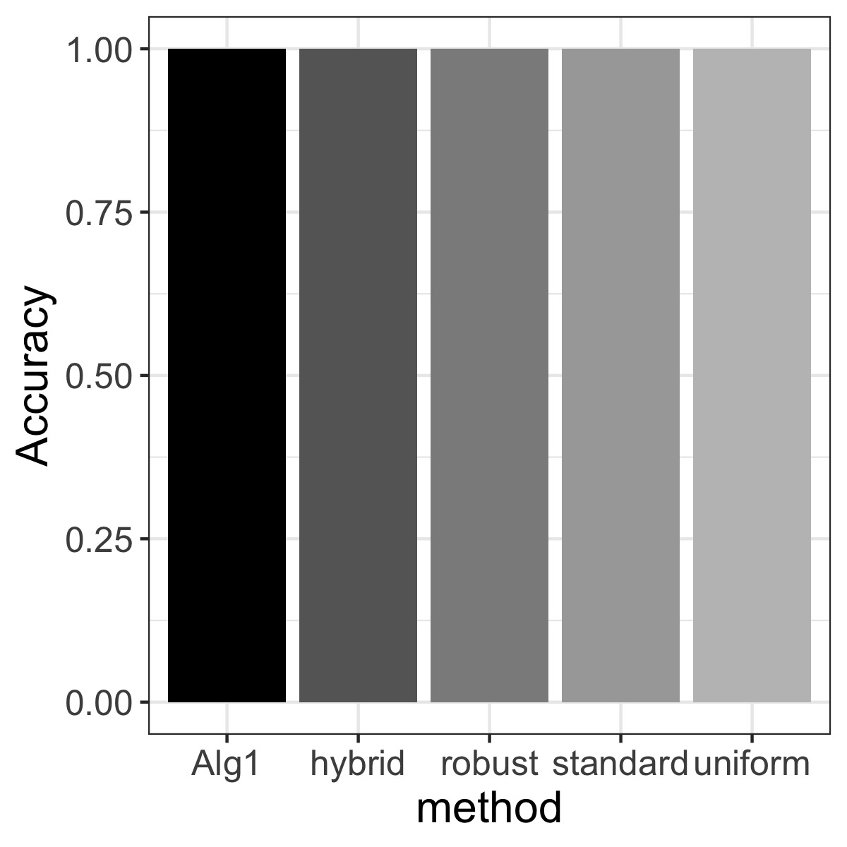
(a) $M_{1}$

(b) $M_{2}$

(c) $M_{3}$

(d) $M_{1}$

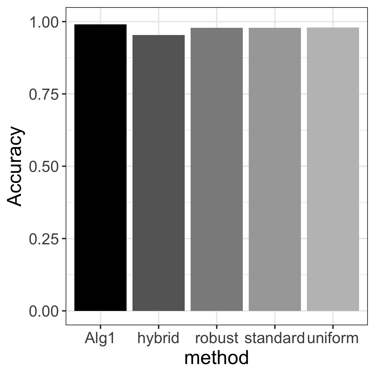
(e) $M_{2}$

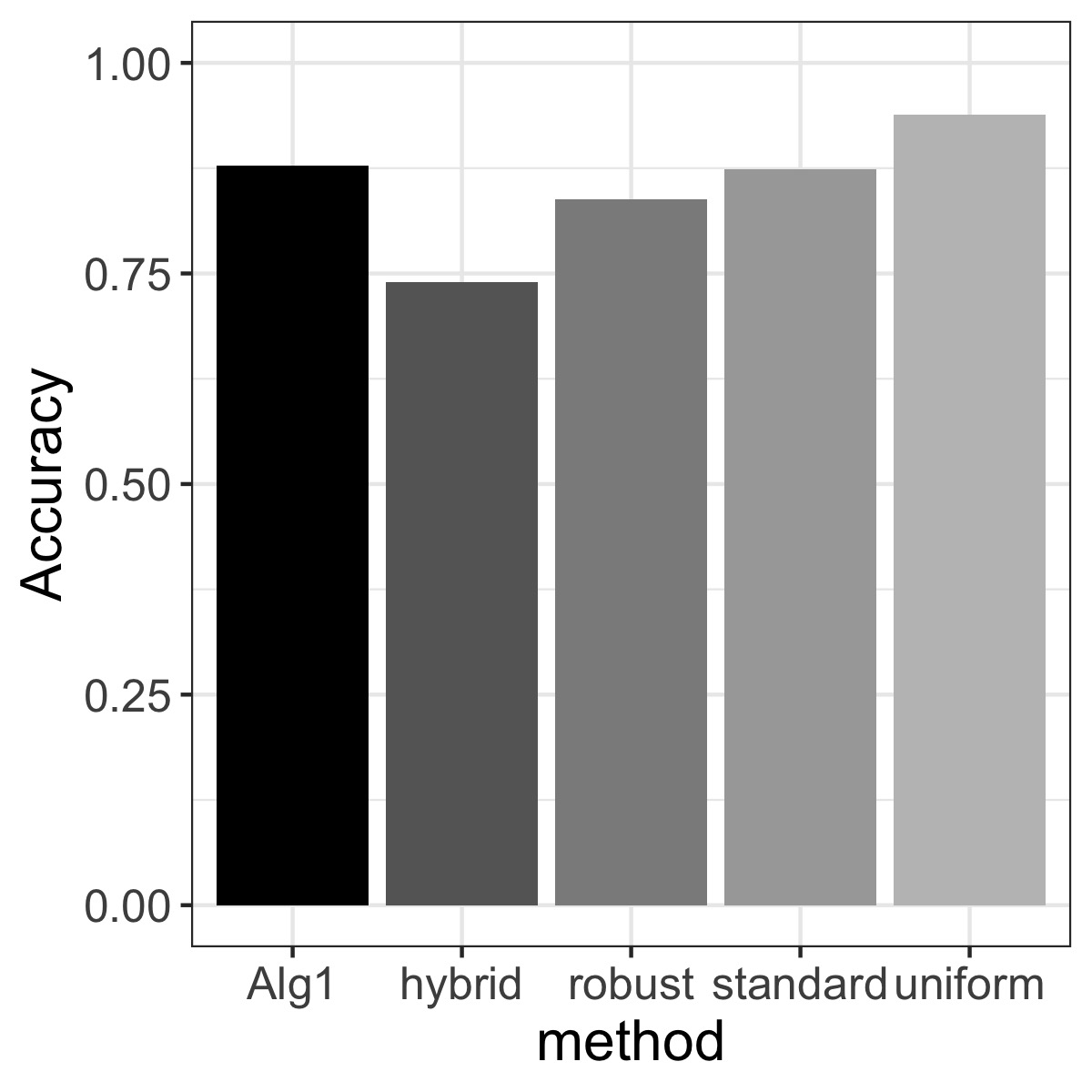
(f) $M_{3}$

Figure 3: Selection accuracy of the BIC based on $150$ observations from different designs in different true models defined by (5.1). Upper part: SNR=3.75; lower part: SNR=1.35.

5.2 Models for robust parameter design

In a robust parameter design, the input variable are divided into two classes: control factors $(\bm{x})$ and noise factors $(\bm{z})$. Control factors refer to the design factors whose values are fixed once they are chosen. Noise factors refers to the design variables that are hard or expansive to control during the user conditions but can be observed. More details can be found in Chapter 11 of Wu and Hamada, (2021). Engineers aim to find a setting of control factors to make it less sensitive to noise variation. We consider a typical example with three control factors and three noise factors and the model

$$M_{\rm full}:Y= \beta_{0}+\beta_{1}x_{1}+\beta_{2}x_{2}+\beta_{3}x_{3}+(\beta_{4}+\beta_{5}x_{1}+\beta_{6}x_{2}+\beta_{7}x_{3})z_{1}$$

$$+(\beta_{8}+\beta_{9}x_{1}+\beta_{10}x_{2}+\beta_{11}x_{3})z_{2}+(\beta_{12}+\beta_{13}x_{1}+\beta_{14}x_{2}+\beta_{15}x_{3})z_{3}+\varepsilon,$$

to explore the response surface and choose the control factor $\bm{x}$ such that the coefficients of $\bm{z}$, for example $\beta_{4}+\beta_{5}x_{1}+\beta_{6}x_{2}+\beta_{7}x_{3}$, $\beta_{8}+\beta_{9}x_{1}+\beta_{10}x_{2}+\beta_{11}x_{3}$, $\beta_{12}+\beta_{13}x_{1}+\beta_{14}x_{2}+\beta_{15}x_{3}$, are close to zero. In practice, one may not known which noise factor has impact to the response. Thus, we consider the following seven reduced model as candidates

$$M_{1}: ~{}Y=\beta_{0}+\beta_{1}x_{1}+\beta_{2}x_{2}+\beta_{3}x_{3}+\varepsilon,$$

$$M_{2}: ~{}Y=\beta_{0}+\beta_{1}x_{1}+\beta_{2}x_{2}+\beta_{3}x_{3}+(\beta_{4}+\beta_{5}x_{1}+\beta_{6}x_{2}+\beta_{7}x_{3})z_{1}+\varepsilon,$$

$$M_{3}: ~{}Y=\beta_{0}+\beta_{1}x_{1}+\beta_{2}x_{2}+\beta_{3}x_{3}+(\beta_{4}+\beta_{5}x_{1}+\beta_{6}x_{2}+\beta_{7}x_{3})z_{2}+\varepsilon,$$

$$M_{4}: ~{}Y=\beta_{0}+\beta_{1}x_{1}+\beta_{2}x_{2}+\beta_{3}x_{3}+(\beta_{4}+\beta_{5}x_{1}+\beta_{6}x_{2}+\beta_{7}x_{3})z_{3}+\varepsilon,$$ (5.3)

$$M_{5}: ~{}Y=\beta_{0}+\beta_{1}x_{1}+\beta_{2}x_{2}+\beta_{3}x_{3}+(\beta_{4}+\beta_{5}x_{1}+\beta_{6}x_{2})z_{1}+(\beta_{7}+\beta_{8}x_{1}+\beta_{9}x_{3})z_{3}+\varepsilon,$$

$$M_{6}: ~{}Y=\beta_{0}+\beta_{1}x_{1}+\beta_{2}x_{2}+\beta_{3}x_{3}+(\beta_{4}+\beta_{5}x_{1}+\beta_{6}x_{2})z_{1}+(\beta_{7}+\beta_{8}x_{2}+\beta_{9}x_{3})z_{3}+\varepsilon,$$

$$M_{7}: ~{}Y=\beta_{0}+\beta_{1}x_{1}+\beta_{2}x_{2}+\beta_{3}x_{3}+(\beta_{4}+\beta_{5}x_{1}+\beta_{6}x_{3})z_{1}+(\beta_{7}+\beta_{8}x_{2}+\beta_{9}x_{3})z_{2}+\varepsilon,$$

where both the control and noise factor vary in the interval $[-1,1]$. In this case, the $D$-optimal design for the model $M_{\rm full}$ is a product designs of two $2^{3}$ full factorial designs with eight replications, and this design is also $D$-optimal for the models $M_{1},\ldots,M_{7}$. However, when model $M_{1}$ is the true model, one can just use a $2^{3}$ full factorial design with only $64$ replications to achieve the same statistical efficiency. Clearly, the later one is more appreciated since it certainly reduces the costs in controlling the noise factors

We now illustrate the application of Algorithm 1, where the total number of experiment units is fixed as $n=512$ and the size $n_{t}$ of observations at each stage $t$ depends on the design we adopt. To be precise, when we choose an optimal design for the models $M_{1},\ldots M_{4}$, at stage $t$, we set $n_{t}=16$. If we choose the optimal design for the models $M_{5},\ldots M_{7}$ we set $n_{t}=32$. When a component $z_{j}$ of $\bm{z}$ is not controlled by the selected design at stage $t$, we assume that it is generated from a uniform distribution on the interval $[\min(x_{j},0),\max(x_{j},0)]$. Since the noise factor can be easily observed, we also assume that the value of $\bm{z}$ will be recorded such that all candidate models are estimable. Therefore we use Algorithm 1 with $\rho_{t}=0$ for all $t$.

The $D$-efficiencies of the sequential design generated by Algorithm 1 are shown in Figure 4 for an increasing total sample size $n$, where the true model is given by $M_{1}$, $M_{2}$, and $M_{5}$. As in Section 5.1, we compare the new method with the robust optimal design which maximize the geometric mean of the $D$-efficiencies in the models $M_{1}-M_{7}$, the uniform design with $64$ support points, and a hybrid design defined by $\sum_{k=1}^{7}7^{-1}\xi_{k}^{*}$.

The uniform design has rather low efficiencies. If model $M_{1}$ is the true model, all other designs have efficiency one. If $M_{2}$ or $M_{5}$ is the true model, the efficiency of the sequential design increases quickly and exceeds the efficiency of the hybrid design already for sample sizes $48$ and $80$ (usually after three or four stages), respectively. Moreover, if the sample size is further increased the efficiency approaches $1$. For example, of $n=256$, the efficiencies of the sequential design are approximately $97\%$, if the true model is given by $M_{2}$ or $M_{5}$.

To further compare the optimal design $\xi^{*}_{\mathrm{true}}$ for the true model and the robust optimal design with the sequential designs generated by Algorithm 1 we evaluate their costs in Figure 5. To be precise, the costs are calculated by $1+5m_{z}$ for each experimental unit where $m_{z}$ is the number of noise factors that are controlled in the corresponding unit. We observe that the new method method has competitive performance with the optimal design $\xi^{*}_{\mathrm{true}}$ for the true model (the $D$-efficiencies are larger than $98\%$). Moreover, the sequential design generated by Algorithm 1 and the design $\xi^{*}_{\mathrm{true}}$ (which can only be used if the true model is known before the experiment)  require a substantially smaller budget compared to the robust optimal design, because this design controls some redundant noise factors.

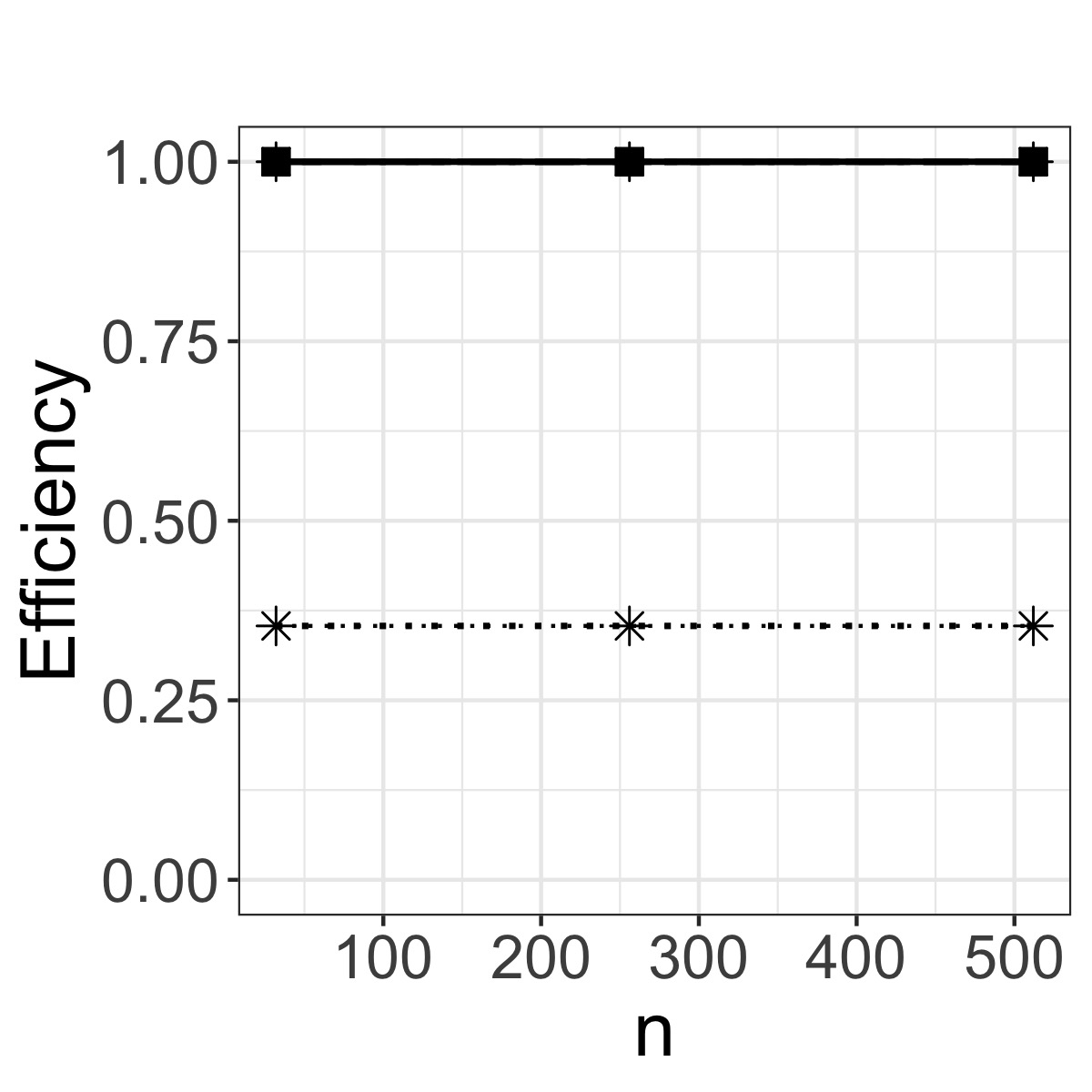
(a) $M_{1}$

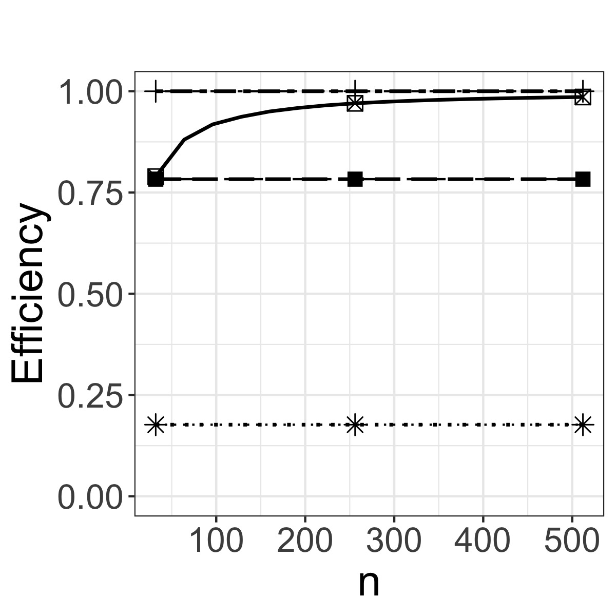
(b) $M_{2}$

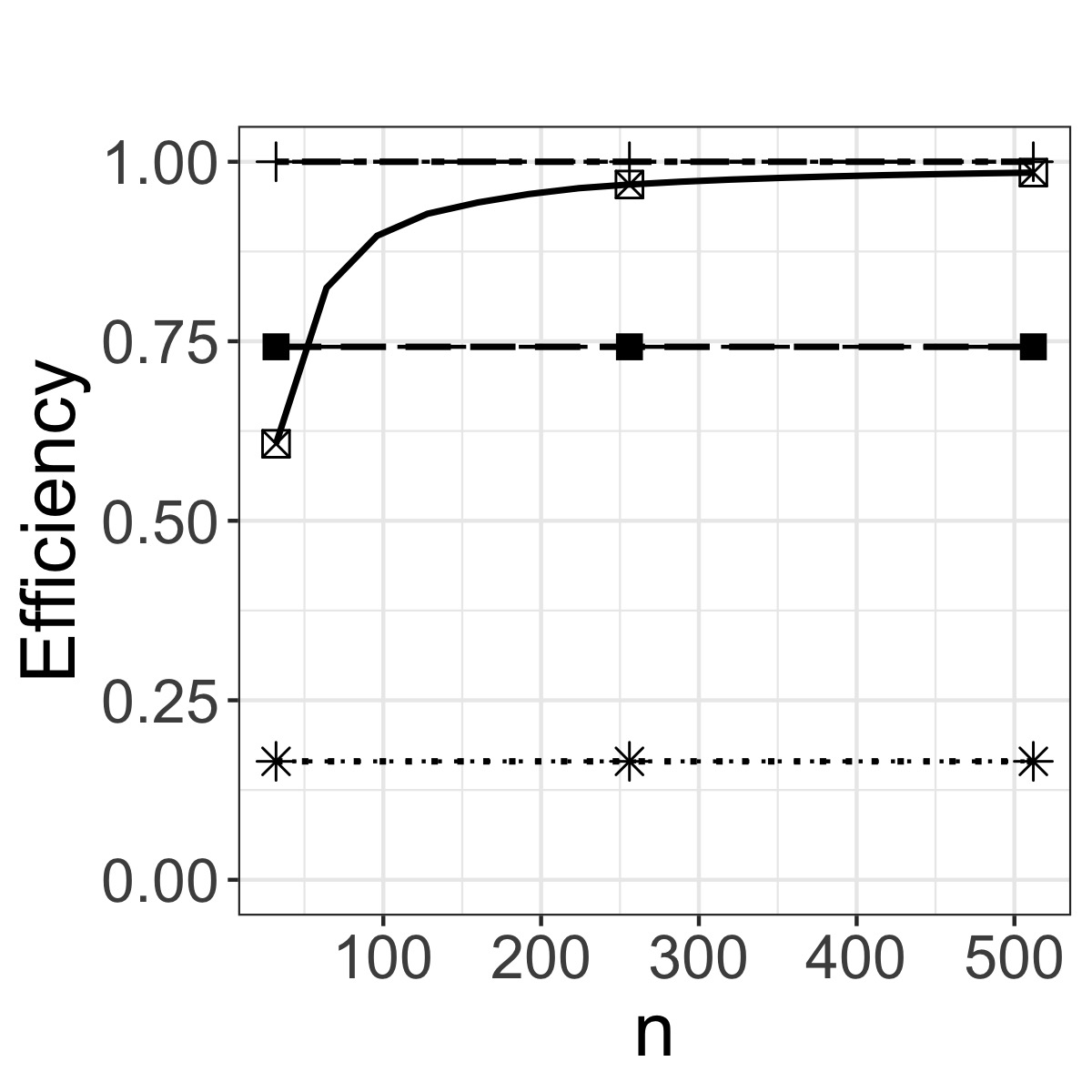
(c) $M_{5}$

Figure 4: $D$-efficiencies (5.2) for the true model as the the total sample size $n$ of the sequential design is increasing. The models are defined by (5.3). Four designs are compared: sequential design constructed by Algorithm 1 ($\boxtimes$); robust design ($+$); uniform design with 64 supports ($\ast$); hybrid design ($\blacksquare$).

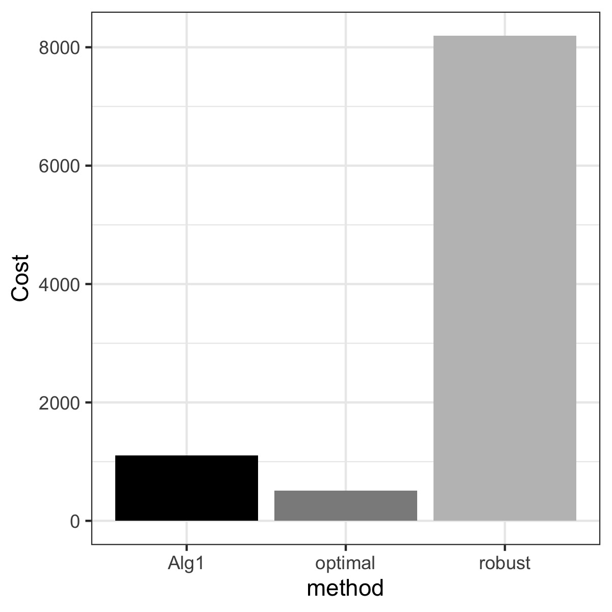
(a) $M_{1}$

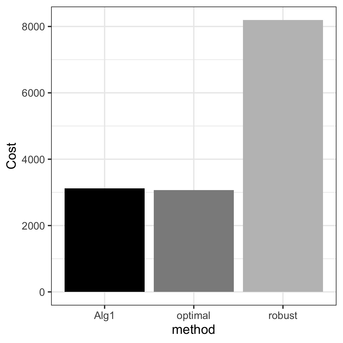
(b) $M_{2}$

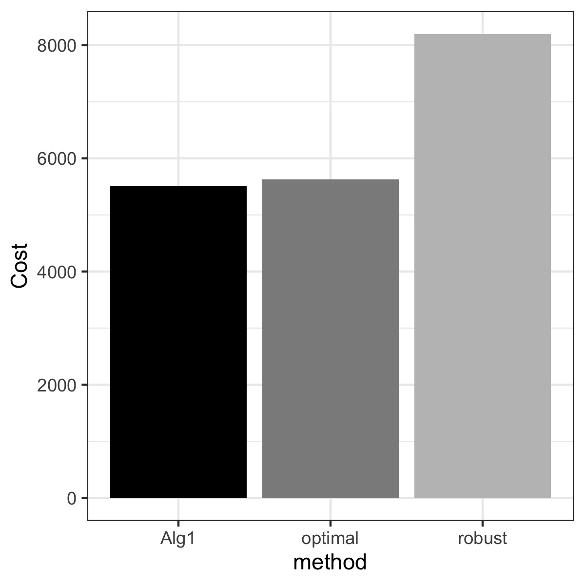
(c) $M_{5}$

Figure 5: Design costs for different methods under $512$ experiment units when $M_{1},M_{2}$, and $M_{5}$ is the true model, respectively. The models are defined by (5.3). Here the results for the uniform design are omitted since the design efficiencies are not comparable with other methods.

5.3 Models with multivariate predictors

In this subsection, we will illustrate how the modified Algorithm 1 according to Remark 3 works. Consider the following six linear regression with the design region ${\cal X}=[-1,1]^{3}$.

$$M_{1}: ~{}~{}Y=\beta_{0}+\beta_{1}x_{1}+\beta_{2}x_{2}+\beta_{3}x_{3}+\varepsilon,$$

$$M_{2}: ~{}~{}Y=\beta_{0}+\beta_{1}x_{1}+\beta_{2}x_{2}+\beta_{3}x_{3}+\beta_{4}x_{1}x_{2}+\beta_{5}x_{3}^{2}+\varepsilon,$$

$$M_{3}: ~{}~{}Y=\beta_{0}+\beta_{1}x_{1}+\beta_{2}x_{2}+\beta_{3}x_{3}+\beta_{4}x_{2}x_{3}+\beta_{5}x_{1}^{2}+\varepsilon,$$ (5.4)

$$M_{4}: ~{}~{}Y=\beta_{0}+\beta_{1}x_{1}+\beta_{2}x_{2}+\beta_{3}x_{3}+\beta_{4}x_{1}x_{2}+\beta_{5}x_{1}x_{3}+\varepsilon,$$

$$M_{5}: ~{}~{}Y=\beta_{0}+\beta_{1}x_{1}+\beta_{2}x_{2}+\beta_{3}x_{3}+\beta_{4}x_{1}x_{2}+\beta_{5}x_{2}x_{3}+\varepsilon,$$

$$M_{6}: ~{}~{}Y=\beta_{0}+\beta_{1}x_{1}+\beta_{2}x_{2}+\beta_{3}x_{3}+\beta_{4}x_{1}x_{2}+\beta_{5}x_{2}x_{3}+\beta_{6}x_{1}x_{3}+\beta_{7}x_{1}^{2}+\beta_{8}x_{2}^{2}+\beta_{9}x_{3}^{2}+\varepsilon.$$

According to Chapter 15.11 of Pukelsheim, (2006), a design with equal masses at the points $(1,1,1),(1,1,-1),(1,-1,1),(1,-1,-1),(-1,1,1),(-1,1,-1),(-1,-1,1)$, and $(-1,-1,-1)$ is D-optimal for model $M_{1},M_{4}$, and $M_{5}$. However, with this design the models $M_{2}$ and $M_{6}$ are not estimable since the quadratic term is the alias of the intercept term. Note that this problem can also be easily solved by Algorithm 1 with a hybrid design but we use the modified algorithm here for illustrative purposes.

Recall that ${\cal D}_{t}=\{(\bm{x}_{n_{0}+\ldots+n_{t-1}+1},Y_{n_{0}+\ldots+n_{t-1}+1}),\ldots,(\bm{x}_{n_{0}+\ldots+n_{t}},Y_{n_{0}+\ldots+n_{t}})\}$ is the set of $n_{t}$ observations taken at stage $t$. We denote by $\bm{\tilde{x}_{ti}},\ldots,\bm{\tilde{x}_{tm}}$ the different experimental conditions in ${\cal D}_{t}$ and by $Y_{tij}$ ($i=1,\ldots,n_{ti}$) the observations taken at each $\bm{\tilde{x}_{ti}}$ ($i=1,\ldots,m$) such that $\sum_{i=1}^{m}n_{ti}=n_{t}$. As suggested in Chapter 2.3 in McCullagh and Nelder, (1989), we use Pearson $\chi^{2}$ statistic

$$\chi^{2}_{t}=\sum_{i=1}^{m}\sum_{j=1}^{n_{ti}}(Y_{tij}-\hat{\mu}_{i,M_{k}})^{2}/\hat{\sigma}^{2},$$

for testing the goodness-of-fit of the plausible model $M_{k}$. Here $\hat{\mu}_{i,M_{k}}$ is the prediction at the point $\bm{\tilde{x}_{ti}}$ using model $M_{k}$ estimated from the data ${\cal D}_{t}$, $\hat{\sigma}^{2}={(n_{t}-m)^{-1}}\sum_{i=1}^{m}\sum_{j=1}^{n_{ti}}(Y_{tij}-\bar{Y}_{ti})^{2}$ is an estimate of the variance and $\bar{Y}_{ti}=n_{i}^{-1}\sum_{j=1}^{n_{ti}}Y_{tij}$.

As in Section 5.1, we also compare the proposed design with a robust design which maximizes the geometric mean of the $D$-efficiencies in model $M_{1}$–$M_{6}$, a hybrid design defined by $6^{-1}\sum_{k=1}^{6}\xi^{*}_{k}$ and a uniform design with $8$ supports. In this example, we set $n_{t}=36$ and $T=15$. The results are shown in Figure 6, where the errors are standard normal distributed and all parameters $\beta_{j}$ are set to one. We observe that for an increasing number of stages the proposed designs are close to the optimal design under the true model in all cases under consideration. This confirms our theoretical findings in in Theorem 1. For models $M_{1}$ and $M_{5}$ the sequential design already outperforms its competitors for small sample sizes. On the other hand, if the true model is the widest model $M_{6}$ and $T$ is relatively small, the robust methods have larger $D$-efficiency since at the beginning the proposed method takes some designs with zero efficiency in true model. This is the price we pay for model exploration.

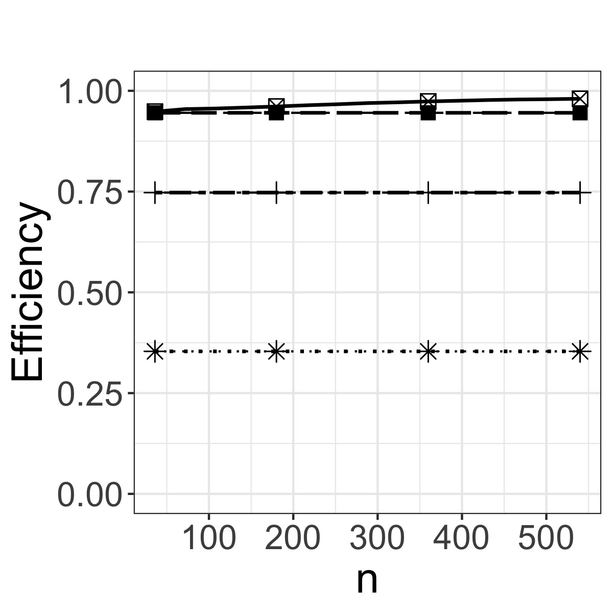
(a) $M_{1}$

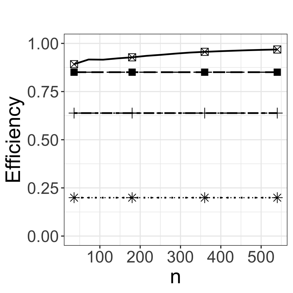
(b) $M_{5}$

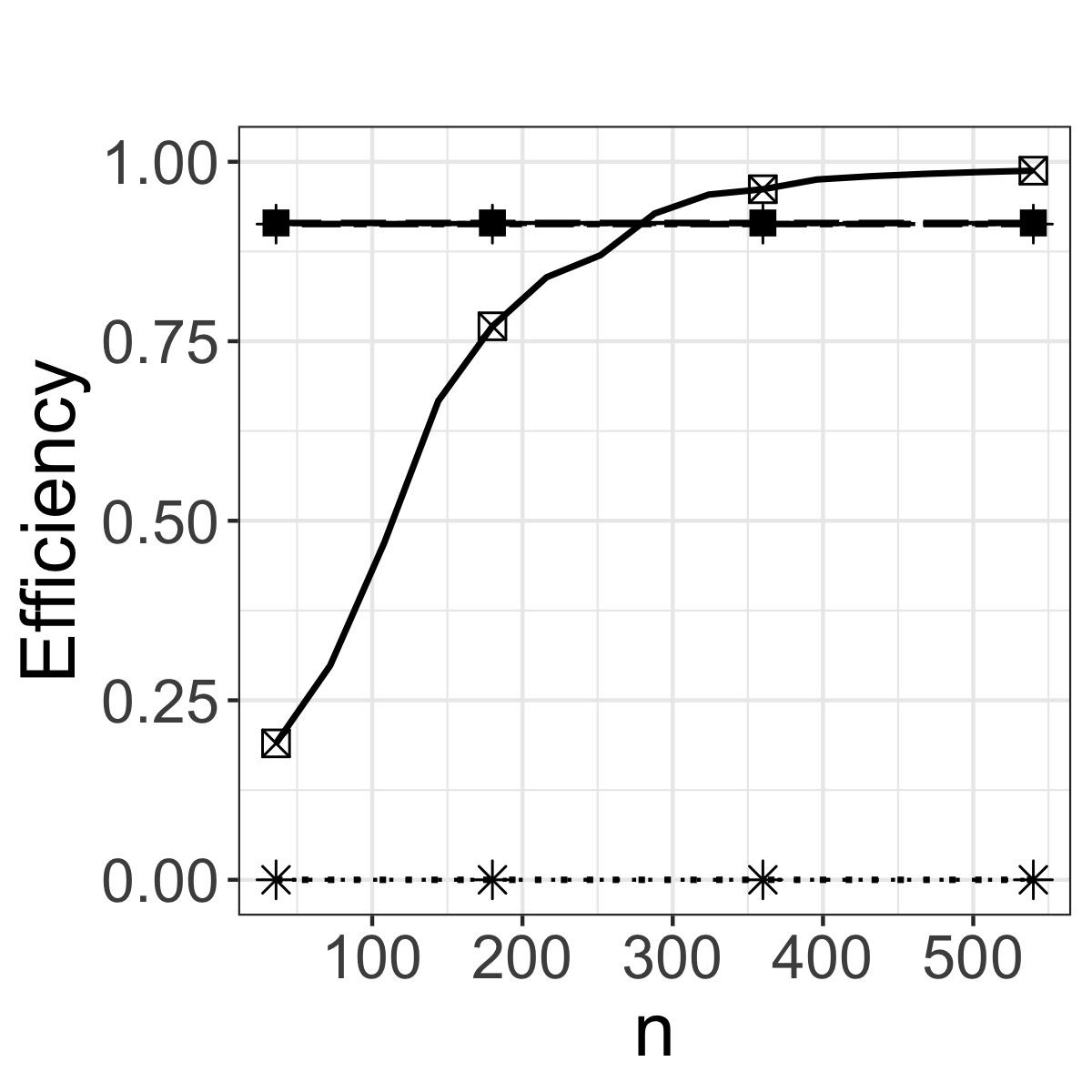
(c) $M_{6}$

Figure 6: $D$-efficiencies (5.2) for the true model as the total sample size $n$ of the sequential design is increasing. The models are defined by (5.4). Four designs are compared: sequential design constructed by the modified Algorithm 1 according to Remark 3 ($\boxtimes$); uniform design with five supports ($\ast$); robust design($+$); and hybrid design ($\blacksquare$).

6 Concluding remarks

Optimal designs are frequently criticized for their dependence on model specification. In practice, it is common to see that several plausible models are available to describe the relation between the predictors and experimental outputs, and the goal is to estimate the parameters in the most appropriate (true) model among the candidate models. Consequently, design of experiments has to take the different goals, most efficient estimation in the true (but unknown) model and identifying the true model, into account. In this paper we address this problem by a reinforcement learning approach and construct sequential designs which achieve a specified balance between estimation and discrimination. The key idea is to feed only a small batch of experimental units at a time and to collect the gains to prioritize a design that is suitable for the true model, i.e., reinforcing the positive outcomes. From a theoretical side we prove that our method provides a sequence of design with efficiencies converging $1$ for the true model. Moreover, we also derive finite sample lower bounds for the expected efficiency in true model, and show that the sequential algorithm also identifies the true model with a probability converging to one. From a practical side we demonstrate by means of a simulation study that the new sequential designs have very good finite sample properties compared to other well-developed design procedures for model discrimination and parameter estimation.

In this paper we concentrate on linear models and locally optimal designs for non-linear models, which require some prior information about the unknown parameters. An interesting direction of future research is the extension of the reinforcement learning approach to construct sequential designs with respect to robust optimality criteria, such as Bayes- maximin-criteria (see, for example Chaloner and Verdinelli,, 1995; Dette,, 1997; Müller and Pázman,, 1998, among many others). Moreover, it would be also interesting to study different strategies in the evaluation step for power improvement.

Acknowledgements. The authors would like to thank Birgit Tormöhlen who typed parts of this manuscript with considerable technical expertise. The work of H. Dette was partially supported by the DFG Research unit 5381 Mathematical Statistics in the Information Age, project number 460867398.

Appendix A Appendix: Technical details

A.1 Proof of the results in Section 4.1

Proof of Theorem 1.

This is a direct result from Theorem 3 (which will be shown later) by letting $T\to\infty$. ∎

Proof of Theorem 2.

The first part comes from the result in Lemma 3 (which will be shown later). For the second part, note the fact that $\sum_{j=1}^{T}N_{j}(T)=T$. Thus it is sufficient to show that $N_{\mathrm{true}}(T)\geq T/2$ with probability approaching one. Without loss of generality, we assume $M_{\mathrm{true}}=M_{1}$. By the Markov’s inequality, it follows that

$$\mathbb{P}(N_{1}(t)<T/2) =\mathbb{P}\Big{(}T-\sum_{j=2}^{\mathrm{K}}N_{j}(t)<T/2\Big{)}=\mathbb{P}\Big{(}\sum_{j=2}^{\mathrm{K}}N_{j}(t)>T/2\Big{)}$$

$$\leq\frac{2}{T}\mathbb{E}\Big{[}\sum_{t=1}^{T}\mathbb{I}(\mathcal{A}(t))\Big{]}\leq\frac{2}{T}(C_{1}\log(T)+C_{2})=o(1),$$

as $T\to\infty$, where $C_{1},C_{2}$ are some constants and the second inequality is a consequence of Lemma 3 (which will be shown later). ∎

A.2 Proof of the results in Section 4.2

In this subsection, we will begin with dealing with the result in Theorems 3. The proof of Theorem 4 is postponed to the end of this section.

A.2.1 Proof of Theorem 3

Before proving Theorem 3, we introduce some addition notations and several auxiliary results. First, we define $\hat{\theta}_{j}(t)=(a_{j}(t)-1)/(t-1)$ for $t>1$ as a “rough estimator” of the posterior probability $\theta_{j}$ in (3.2) and define $\hat{\theta}_{j}(1)=0$ for all $j$. We further introduce the following three events

$$\mathcal{B}(t) =\left\{\hat{\theta}_{\mathrm{true}}(t)\leq c+\frac{\alpha}{2}\text{ or }\exists M_{j}\neq M_{\mathrm{true}}\text{ s.t. }\hat{\theta}_{j}(t)\geq c-\frac{\alpha}{2}\right\},$$ (A.1)

$$\mathcal{C}(t) =\left\{\hat{\theta}_{\mathrm{true}}(t)-\eta_{\mathrm{true}}(t)\geq\frac{\alpha}{2}\text{ or }\exists M_{j}\neq M_{\mathrm{true}}\text{ s.t. }\eta_{j}(t)-\hat{\theta}_{j}(t)\geq\frac{\alpha}{2}\right\},$$ (A.2)

$$\mathcal{D}(t) =\Big{\{}t>\frac{8\log(T)}{\alpha^{2}}+1\Big{\}}.$$ (A.3)

Lemma 1.

Under Condition 1, it holds that

$$\mathscr{R}_{1}(T):=\sum_{t=1}^{T}\mathbb{E}(\mathbb{I}(\mathcal{A}(t)\cap\mathcal{B}(t)))\leq\mathrm{K}\Big{(}1+\frac{2}{\alpha^{2}}\Big{)}.$$ (A.4)

Proof of Lemma 1.

The risk $\mathscr{R}_{1}(T)$ can be decomposed as

$$\mathscr{R}_{1}(T)\leq\mathbb{E}\Big{[}\sum_{t=1}^{T}\mathbb{I}\left(\hat{\theta}_{\mathrm{true}}(t)\leq{c}+\frac{\alpha}{2}\right)\Big{]}+\sum_{M_{j}\neq M_{\mathrm{true}}}\mathbb{E}\Big{[}\sum_{t=1}^{T}\mathbb{I}\left(\hat{\theta}_{j}(t)\geq{c}-\frac{\alpha}{2}\right)\Big{]}$$ (A.5)

and for the sake of brevity, we only deal with the first term showing that

$$\mathbb{E}\Big{[}\sum_{t=1}^{T}\mathbb{I}\left(\hat{\theta}_{\mathrm{true}}(t)\leq c+\frac{\alpha}{2}\right)\Big{]}\leq 1+\frac{2}{\alpha^{2}}.$$ (A.6)

The inequality for the second term in (A.5) can be obtained analogously. With the definition of $\theta_{j}(\xi_{t}^{\rm hyb})$ we denote by

$$\bar{\theta}_{j}(t) =\frac{1}{t-1}\sum_{k=1}^{t-1}\theta_{j}(\xi_{(k)}^{\rm hyb})=\frac{1}{t-1}\sum_{k=1}^{t-1}\theta_{j}(\rho_{k}\xi_{\tau_{k}}^{*}+(1-\rho_{k})\xi_{\rm unif})$$

$$=\frac{1}{t-1}\sum_{k=1}^{t-1}\mathbb{E}[\zeta_{j}(t)]=\frac{1}{t-1}\mathbb{E}[a_{j}(t)-1]=\mathbb{E}[\hat{\theta}_{j}(t)]$$

the expectation of $\hat{\theta}(t)$ for $t=2,\ldots,T$. Simple calculations and Condition 1 yield that (note that $\hat{\theta}_{\mathrm{true}}(1)=0$ and $\bar{\theta}_{\mathrm{true}}(t)>c+\alpha$ for all $t>1$)

$$\mathbb{E}\Big{[}\sum_{t=1}^{T}\mathbb{I}(\hat{\theta}_{\mathrm{true}}(t)\leq c+\alpha/2)\Big{]}= 1+\sum_{t=2}^{T}\mathbb{P}\left(\hat{\theta}_{{\mathrm{true}}}(t)-\bar{\theta}_{{\mathrm{true}}}(t)\leq c+\alpha/2-\bar{\theta}_{\mathrm{true}}(t)\right)$$

$$\leq 1+\sum_{t=2}^{T}\mathbb{P}\left(\hat{\theta}_{{\mathrm{true}}}(t)-\bar{\theta}_{{\mathrm{true}}}(t)\leq-\alpha/2\right)$$

$$\leq 1+\sum_{t=1}^{T}\exp\left(-t\alpha^{2}/2\right)\leq 1+\sum_{t=1}^{\infty}\exp\left(-t\alpha^{2}/2\right)$$

$$\leq 1+\frac{\exp\left(-\alpha^{2}/2\right)}{1-\exp\left(-\alpha^{2}/2\right)}<1+\frac{2}{\alpha^{2}},$$

where we have used Hoeffding’s inequality and the last inequality comes from the fact that $1/(\exp(x)-1)<1/x$. This yields (A.6). The second term can be bounded analogously, which concludes the proof of this Lemma. ∎

Lemma 2.

The following bound holds when the Algorithm 1 is applied.

$$\mathscr{R}_{2}(T):=\sum_{t=1}^{T}\mathbb{E}\{\mathbb{I}(\mathcal{A}(t)\cap\mathcal{B}^{c}(t)\cap\mathcal{C}(t)\cap\mathcal{D}(t))\}\leq\mathrm{K}.$$ (A.7)

Proof of Lemma 2.

For the indices in the set $\mathcal{D}(t)$ we have $t-1>{8\log(T)}/{\alpha^{2}}$, which implies ${\alpha}/{2}>\big{(}{2\log(T)}/({t-1})\big{)}^{1/2}$. The event $\mathcal{B}^{c}(t)\cap\mathcal{C}(t)\cap\mathcal{D}(t)\subseteq\mathcal{C}(t)\cap\mathcal{D}(t)$ is then a subset of

$$\Big{\{}\exists M_{j}\neq M_{\mathrm{true}}:\eta_{j}(t)-\hat{\theta}_{j}(t)\geq\Big{(}{\frac{2\log(T)}{{t-1}}}\Big{)}^{1/2}~{}\text{or}~{}~{}~{}\hat{\theta}_{\mathrm{true}}(t)-\eta_{\mathrm{true}}(t)\geq\Big{(}{\frac{2\log(T)}{{t-1}}}\Big{)}^{1/2}\Big{\}}.$$

As $\hat{\theta}_{j}(t)=(a_{j}(t)-1)/(t-1)=(a_{j}(t)-1)/(a_{j}(t)+b_{j}(t)-2)$ is the mode of a random variable sampled from a $\mathrm{Beta}(a_{j}(t),b_{j}(t))$ distribution, we can use Lemma 4 in Wang and Chen, (2018) to obtain the bound

$$\sum_{t=1}^{T}\mathbb{P}\left(\mathcal{A}(t)\cap\mathcal{B}^{c}(t)\cap\mathcal{C}(t)\cap\mathcal{D}(t)\right) \leq\sum_{t=1}^{T}\mathbb{P}\left(\mathcal{B}^{c}(t)\cap\mathcal{C}(t)\cap\mathcal{D}(t)\right)\leq\mathrm{K},$$

which gives the desired result. ∎

Our next result provides a bound on the expected number of times that the event $\mathcal{A}(t)=\{M_{\tau_{t}}\neq M_{\mathrm{true}}\}$ happens for $t=1,\ldots,T$.

Lemma 3.

If Condition 1 is satisfied and all models are estimable under the design selected by Algorithm 1, we have

$$\mathbb{E}\Big{[}\sum_{t=1}^{T}\mathbb{I}\left(\mathcal{A}(t)\right)\Big{]}\leq\mathrm{K}\Big{(}2+\frac{2}{\alpha^{2}}\Big{)}+\frac{8\log(T)}{\alpha^{2}}.$$ (A.8)

Proof of Lemma 3.

We use the decomposition

$$\mathbb{I}\left(\mathcal{A}(t)\right) =\mathbb{I}\left(\mathcal{A}(t)\cap\mathcal{B}(t)\right)+\mathbb{I}\left(\mathcal{A}(t)\cap\mathcal{B}^{c}(t)\cap\mathcal{C}(t)\right)+\mathbb{I}\left(\mathcal{A}(t)\cap\mathcal{B}^{c}(t)\cap\mathcal{C}^{c}(t)\right).$$ (A.9)

and derive bounds for the three terms separately.

The first term has already been considered in Lemma 1. For the second term we use a further decomposition

$$\mathbb{I}\left(\mathcal{A}(t)\cap\mathcal{B}^{c}(t)\cap\mathcal{C}(t)\right) =\mathbb{I}\left(\mathcal{A}(t)\cap\mathcal{B}^{c}(t)\cap\mathcal{C}(t)\cap\mathcal{D}(t)\right)+\mathbb{I}\left(\mathcal{A}(t)\cap\mathcal{B}^{c}(t)\cap\mathcal{C}(t)\cap\mathcal{D}^{c}(t)\right).$$

To evaluate the second term of the above equality, note that the worst scenario appears in the case where the designs selected in the first $t\leq 8\log(T)/\alpha^{2}$ stages are all incorrect, which implies for the corresponding risk

$$\mathbb{E}\Big{[}\sum_{t=1}^{T}\mathbb{I}\left(\mathcal{A}(t)\cap\mathcal{B}^{c}(t)\cap\mathcal{C}(t)\cap\mathcal{D}^{c}(t)\right)\Big{]}\leq 8\log(T)/\alpha^{2}.$$

Now, an application of Lemma 2 gives

$$\mathbb{E}\Big{[}\sum_{t=1}^{T}\mathbb{I}\left(\mathcal{A}(t)\cap\mathcal{B}^{c}(t)\cap\mathcal{C}(t)\right)\Big{]}\leq\mathrm{K}+8\log(T)/\alpha^{2}$$

Finally, we deal with the last term in (A.9). Note that

$$\mathcal{B}^{c}(t)\cap\mathcal{C}^{c}(t){=}\big{\{}{\eta_{\mathrm{true}}}(t)>c~{}\text{and}~{}\forall M_{j}\neq M_{\mathrm{true}}\,\,\,\,{\eta_{j}(t)}<c\big{\}},$$

which implies that ${\eta_{\mathrm{true}}}(t)$ corresponds to the largest value among all $\{\eta_{j}(t)\}_{j=1}^{\mathrm{K}}$ at stage $t$. In other words Algorithm 1, selects the optimal design under the true model, which means that $\mathcal{A}^{c}(t)$ happens at stage $t$. Thus, $\mathbb{I}(\mathcal{A}(t)\cap\mathcal{B}^{c}(t)\cap\mathcal{C}^{c}(t))=0$, and the desired result follows by combining the estimates for the three terms in (A.9). ∎

Proof of Theorem 3.

Recall that the number of runs in each stage is the same, which implies $n_{t}/n=1/T$ and that $\rho_{t}=N_{\tau_{t}}(t)/(N_{\tau_{t}}(t)+1)$, where ${\tau_{t}}$ denotes the index of the model selected at stage $t$ and $N_{j}(t)$ is the number of times that design $\xi_{j}^{*}$ was chosen in the first $t$ stages. Using the concavity of the criterion function $\phi_{\mathrm{true}}(\cdot)$ yields

$$\mathrm{Eff}_{\mathrm{true}}(\xi_{\mathcal{M},T}) =\frac{\phi_{\mathrm{true}}(\xi_{\mathcal{M},T})}{\phi_{\mathrm{true}}(\xi_{\mathrm{true}}^{*})}=\frac{\phi_{\mathrm{true}}(\sum_{t=1}^{T}{T}^{-1}\{\rho_{t}\xi^{*}_{\tau_{t}}+(1-\rho_{t})\xi_{\rm unif}\})}{\phi_{\mathrm{true}}(\xi_{\mathrm{true}}^{*})}$$

$$\geq\frac{\frac{1}{T}\sum_{t=1}^{T}\rho_{t}\phi_{\mathrm{true}}(\xi^{*}_{\tau_{t}})}{\phi_{\mathrm{true}}(\xi_{\mathrm{true}}^{*})}\geq\frac{1}{T}\sum_{t=1}^{T}\rho_{t}\mathbb{I}\left(\mathcal{A}^{c}(t)\right)$$

$$=\frac{1}{T}\sum_{t=1}^{T}\left(1-\frac{1}{N_{\mathrm{true}}(t)+1}\right)\mathbb{I}\left(\mathcal{A}^{c}(t)\right)\geq\frac{1}{T}\sum_{t=1}^{T}\mathbb{I}\left(\mathcal{A}^{c}(t)\right)-\frac{1}{T}\sum_{t=1}^{T}\frac{1}{t}$$

$$\geq\frac{1}{T}\sum_{t=1}^{T}\left(1-\mathbb{I}\left(\mathcal{A}(t)\right)\right){-}\frac{1}{T}\log(T),$$

where the second last third inequality follows from the fact that $1/2+1/3+\cdots+1/(N_{\mathrm{true}}(T)+1)\leq 1+1/2+\cdots+1/T$, since $N_{\mathrm{true}}(T)\leq T$. Thus the result follows immediately from Lemma 3.

A.2.2 Proof of Theorem 4

Note that in the situation considered in Theorem 4 only a part of the models can be examined at stage $t$. To obtain the parallel results of Lemmas 1–3, we denote by $\mathrm{N}_{\rm check}^{(j)}(t):=a_{j}(t)+b_{j}(t)-2$ $(j=1,\ldots,\mathrm{K})$ the number of times that the $j$th model has been checked, and define $\hat{\theta}_{j}(t)=(a_{j}(t)-1)/(a_{j}(t)+b_{j}(t)-2)$ for $j=1,\ldots,\mathrm{K}$ (note that in the situation considered in Theorem 3 we have $\hat{\theta}_{j}(t)=t-1$). Recall that

$$\mathcal{A}(t) =\{M_{\tau_{t}}\neq M_{\mathrm{true}}\}=\left\{\xi_{(t)}^{\rm hyb}\neq\rho_{t}\xi^{*}_{\mathrm{true}}+(1-\rho_{t})\xi_{\rm unif}\right\},$$

$$\mathcal{C}(t) =\left\{\hat{\theta}_{\mathrm{true}}(t)-\eta_{\mathrm{true}}(t)\geq\frac{\alpha}{2}\text{ or }\exists M_{j}\neq M_{\mathrm{true}}\text{ s.t. }\eta_{j}(t)-\hat{\theta}_{j}(t)\geq\frac{\alpha}{2}\right\},$$

and redefine the events

$$\mathcal{B}(t)= \Big{\{}M_{\mathrm{true}}\text{ can be checked under design }\xi_{(t)}^{\rm hyb},~{}~{}\hat{\theta}_{\mathrm{true}}(t)\leq c+\frac{\alpha}{2}\Big{\}}$$

$$\bigcup\Big{\{}~{}\exists M_{j}\text{ can be checked under design }\xi_{(t)}^{\rm hyb},\text{ and }M_{j}\neq M_{\mathrm{true}}\text{ s.t. }\hat{\theta}_{j}(t)\geq c-\frac{\alpha}{2}\Big{\}},$$

$${\mathcal{D}}(t)= \bigcap_{j\in\{1,\ldots,k\}}\Big{\{}\mathrm{N}_{\rm check}^{(j)}(t)>\frac{8\log(T)}{\alpha^{2}}\Big{\}}$$

Note that $\mathrm{N}_{\rm check}^{(j)}(t)={t-1}$ and the models can always be checked for the case we studied in Lemma 1. Therefore we still use notations $\mathcal{B}(t)$ and ${\mathcal{D}}(t)$ for the ease of presentation. According to the construction of $\xi_{(t)}^{\rm hyb}$, one can expect that the model $M_{\tau_{t}}$ can be checked for $t=1,\ldots,T$, since $M_{\tau_{t}}$ is estimable under $\xi_{\tau_{t}}^{*}$ and a uniform design provide additional design points for model checking. On the other hand, if a model $M_{j}$ can not be checked at stage $t$, we have $\xi_{(t)}^{\rm hyb}\neq\rho_{t}\xi^{*}_{j}+(1-\rho_{t})\xi_{\rm unif}$, i.e., $M_{\tau_{t}}\neq M_{j}$ at stage $t$.

Lemma 4.

Under Condition 2, we have

$$\mathscr{R}_{1}(T):=\sum_{t=1}^{T}\mathbb{E}(\mathbb{I}(\mathcal{A}(t)\cap\mathcal{B}(t)))\leq\mathrm{K}\Big{(}1+\frac{2}{\alpha^{2}}\Big{)}.$$ (A.10)

Proof of Lemma 4.

Note that

$$\mathscr{R}_{1}(T)\leq ~{}\mathbb{E}\Big{[}\sum_{t=1}^{T}\mathbb{I}\Big{(}M_{\mathrm{true}}\text{ can be checked under }\xi_{(t)}^{\rm hyb},~{}\hat{\theta}_{\mathrm{true}}(t)\leq c+\frac{\alpha}{2}\Big{)}\Big{]}$$

$$~{}+\sum_{M_{j}\neq M_{\mathrm{true}}}\mathbb{E}\Big{[}\sum_{t=1}^{T}\mathbb{I}\Big{(}M_{j}\text{ can be checked under }\xi_{(t)}^{\rm hyb},~{}\hat{\theta}_{j}(t)\geq c-\frac{\alpha}{2}\Big{)}\Big{]}.$$

As in the proof of Lemma 1, we show for the first term

$$\mathbb{E}\Big{[}\sum_{t=1}^{T}\mathbb{I}\left(M_{\mathrm{true}}\text{ can be checked under }\xi_{(t)}^{\rm hyb},~{}\hat{\theta}_{\mathrm{true}}(t)\leq c+\frac{\alpha}{2}\right)\Big{]}\leq 1+\frac{2}{\alpha^{2}}$$ (A.11)

and a similar inequality for the second term proves the result. For this purpose we introduce the notation

$$\bar{\theta}_{j}(t)=\frac{1}{\mathrm{N}_{\rm check}^{(j)}(t)}\sum_{k=1}^{t}\mathbb{I}(M_{j}~{}\text{is checked at stage}~{}k)\theta_{j}(\xi_{(k)}^{\rm hyb})$$

and a decomposition of the time interval $(0,T]=(\iota_{0},\iota_{1}]\cup(\iota_{1},\iota_{2}]\cup\ldots$, where $0=\iota_{0}<\iota_{1}<\iota_{2}<\ldots$ are the times where model $M_{\mathrm{true}}$ has been checked. Note that in each time interval $(\iota_{\ell},\iota_{\ell+1}]$ the model $M_{\mathrm{true}}$ can only be checked once. Recall that the model $M_{\mathrm{true}}$ will be checked if it can be checked according to the modification of Algorithm 1 in Remark 3. For $0<\iota_{w-1}<\iota_{w}\leq T$ we have

$$\mathbb{E}\Big{[}\sum_{t=\iota_{w-1}+1}^{\iota_{w}}\mathbb{I}(M_{\mathrm{true}}\text{ can be checked under }\xi_{(t)}^{\rm hyb},~{}\hat{\theta}_{\mathrm{true}}(t)<c+\alpha/2)\Big{]}$$

$$~{}~{}=\sum_{\iota_{1}<\ldots<\iota_{w-1}}\mathbb{P}\Big{(}M_{\mathrm{true}}\text{ has been checked at}~{}\iota_{1},\iota_{2},\ldots,\iota_{w},~{}\hat{\theta}_{\mathrm{true}}(\iota_{w})<c+\alpha/2\Big{)}$$

$$~{}~{}\leq\sum_{\iota_{1}<\ldots<\iota_{w-1}}\mathbb{P}\left(\hat{\theta}_{\mathrm{true}}(\iota_{w})-\bar{\theta}_{{\mathrm{true}}}(\iota_{w})<-\alpha/2|M_{\mathrm{true}}\text{ has been checked at}~{}\iota_{1},\iota_{2},\ldots,\iota_{w}\right)$$

$$~{}~{}~{}~{}~{}~{}~{}\times\mathbb{P}(M_{\mathrm{true}}\text{ has been checked at}~{}\iota_{1},\iota_{2},\ldots,\iota_{w})$$

$$~{}~{}\leq\exp\left(-w\alpha^{2}/2\right)\sum_{\iota_{1}<\ldots<\iota_{w-1}}\mathbb{P}(M_{\mathrm{true}}\text{ has been checked at}~{}\iota_{1},\iota_{2},\ldots,\iota_{w})$$

$$~{}~{}\leq\exp\left(-w\alpha^{2}/2\right).$$ (A.12)

Here the second inequality is a consequence of Condition 2 and Hoeffding’s inequality by observing that

$$\bar{\theta}_{{\mathrm{true}}}(\iota_{w})=\mathbb{E}[\hat{\theta}_{{\mathrm{true}}}(\iota_{w})|M_{\mathrm{true}}\text{ has been checked at}~{}\iota_{1},\iota_{2},\ldots,\iota_{w}].$$

As $\sum_{\iota_{1}<\ldots<\iota_{w-1}}\mathbb{P}(M_{\mathrm{true}}\text{ has been checked at}$ $~{}\iota_{1},\iota_{2},\ldots,\iota_{w})$ equals to the marginal probability $\mathbb{P}(M_{\mathrm{true}}\text{ has been checked at}~{}\iota_{w})$, which can not exceed one, the last inequality holds as well.

Let $n_{\iota}\leq T$ denote the number of times that model $M_{\mathrm{true}}$ has been checked, then conditioning on the event $\{n_{\iota}>0\}$ and using (A.12) yields

$$\mathbb{E}\Big{[}\sum_{t=1}^{T}\mathbb{I}\left(M_{\mathrm{true}}\text{ can be checked under }\xi_{(t)}^{\rm hyb},~{}\hat{\theta}_{\mathrm{true}}(t)<c+\alpha/2\right)\Big{]}$$

$$~{}~{}~{}~{}\leq\mathbb{E}\Big{[}\sum_{w=0}^{n_{\iota}-1}\mathbb{E}\Big{[}\sum_{t=\iota_{w}+1}^{\iota_{w+1}}\mathbb{I}\left(M_{\mathrm{true}}\text{ can be checked under }\xi_{(t)}^{\rm hyb},~{}\hat{\theta}_{\mathrm{true}}(t)<c+\alpha/2\right)\Big{|}n_{\iota}\geq 1\Big{]}\Big{]}$$

$$~{}~{}~{}~{}~{}~{}~{}~{}~{}+\mathbb{P}(n_{\iota}=0)$$

$$~{}~{}~{}~{}\leq 1+\sum_{w=1}^{\infty}\exp\left(-w\alpha^{2}/2\right)=1+\frac{\exp\left(-\alpha^{2}/2\right)}{1-\exp\left(-\alpha^{2}/2\right)}\leq 1+\frac{2}{\alpha^{2}}~{},$$

which proves (A.11). ∎

Lemma 5.

Under Condition 2 we have

$$\mathscr{R}_{2}(T):=\sum_{t=1}^{T}\mathbb{E}\{\mathbb{I}(\mathcal{A}(t)\cap\mathcal{B}^{c}(t)\cap\mathcal{C}(t)\cap\mathcal{D}(t))\}\leq\mathrm{K}.$$

Proof.

On the event ${\mathcal{D}}(t)$, we have ${\alpha}/{2}>\sqrt{{2\log(T)}/{\mathrm{N}_{\rm check}^{(j)}(t)}}$ for all $j=1,\ldots,\mathrm{K}$. The event $\mathcal{B}^{c}(t)\cap\mathcal{C}(t)\cap{\mathcal{D}}(t)$ is a subset of

$$\Big{\{}\exists M_{j}\neq M_{\mathrm{true}}:\eta_{j}(t)-\hat{\theta}_{j}(t)>\sqrt{\frac{2\log(T)}{\mathrm{N}_{\rm check}^{(j)}(t)}}\text{ or }\hat{\theta}_{\mathrm{true}}(t)-\eta_{\mathrm{true}}(t)>\sqrt{\frac{2\log(T)}{\mathrm{N}_{\rm check}^{(j)}(t)}}\Big{\}},$$

with $\mathrm{N}_{\rm check}^{(i)}(t)\geq 1$. Observing that $\mathrm{N}_{\rm check}^{(j)}(t)=a_{j}(t)+b_{j}(t)-2$. and using Lemma 4 in Wang and Chen, (2018) we obtain

$$\sum_{t=1}^{T}\mathbb{P}\left(\mathcal{A}(t)\cap\mathcal{B}^{c}(t)\cap\mathcal{C}(t)\cap{\mathcal{D}}(t)\right) \leq\sum_{t=1}^{T}\mathbb{P}\left(\mathcal{B}^{c}(t)\cap\mathcal{C}(t)\cap{\mathcal{D}}(t)\right)\leq\mathrm{K},$$

which is the desired result.

∎

Lemma 6.

Assume that Condition 2 holds and that Algorithm 1 is modified according to Remark 3, then

$$\mathbb{E}\Big{[}\sum_{t=1}^{T}\mathbb{I}\Big{(}\mathcal{A}(t)\Big{)}\Big{]}\leq\mathrm{K}\left(3+\frac{4}{\alpha^{2}}+\frac{8\log(T)}{\alpha^{2}}\right).$$ (A.13)

Proof of Lemma 6.

We use the decomposition

$$\mathbb{I}\left(\mathcal{A}(t)\right) =\mathbb{I}\left(\mathcal{A}(t)\cap\mathcal{B}(t)\right)+\mathbb{I}\left(\mathcal{A}(t)\cap\mathcal{B}^{c}(t)\cap\mathcal{C}(t)\right)+\mathbb{I}\left(\mathcal{A}(t)\cap\mathcal{B}^{c}(t)\cap\mathcal{C}^{c}(t)\right)$$

and consider the three terms separately, where the first term has already been considered in the proof of Lemma 4 and the last term is zero.

Thus we focus on the second term, which is further decomposed

$$\mathbb{I}\left(\mathcal{A}(t)\cap\mathcal{B}^{c}(t)\cap\mathcal{C}(t)\right) =\mathbb{I}\left(\mathcal{A}(t)\cap\mathcal{B}^{c}(t)\cap\mathcal{C}(t)\cap{\mathcal{D}}(t)\right)$$

$$+\mathbb{I}\left(\mathcal{A}(t)\cap\mathcal{B}^{c}(t)\cap\mathcal{C}(t)\cap{\mathcal{D}}^{c}(t)\right).$$ (A.14)

According to Lemma 5 the first term is bounded by $\mathrm{K}$, and it remains to consider the second term of (A.14). Note that $\mathcal{A}(t)\cap\mathcal{B}^{c}(t)\cap\mathcal{C}(t)\cap\mathcal{D}^{c}(t)\subseteq\mathcal{A}(t)\cap\mathcal{D}^{c}(t)$. As only one arm is selected at time $t$ and $M_{j}$ can be checked when $\xi^{*}_{j}$ is chosen to construct the hybrid design, the number of times where $\xi^{*}_{j}$ is chosen to construct the hybrid design either exceeds $8\log(T)/\alpha^{2}$ times or not. Observing that that $N_{j}(t)\leq\mathrm{N}_{\rm check}^{(j)}(t)$, it follows $\mathcal{D}^{c}(t)\subset\{\exists~{}j\text{ such that }N_{j}(t)\leq 8\log(T)/\alpha^{2}\}$. Thus, for any $M_{j}\neq M_{\mathrm{true}}$, the total risk caused by the selection is bounded $8\log(T)/\alpha^{2}$ if $N_{j}(t)\leq 8\log(T)/\alpha^{2}$. Otherwise, if $N_{j}(t)>8\log(T)/\alpha^{2}$, the same arguments as given in the proof of Lemma 2 show that the accumulated risk from $t$ to $T$ is bounded by $1$. Therefore, we have

$$\mathbb{E}\left[\mathbb{I}\left(\mathcal{A}(t)\cap\mathcal{B}^{c}(t)\cap\mathcal{C}(t)\cap\mathcal{D}^{c}(t)\right)\right]\leq (\mathrm{K}-1)+8(\mathrm{K}-1)\log(T)/\alpha^{2},$$

and the desired result follows. ∎

Proof of Theorem 4.

The proof now follows by the same arguments as given in the proof of Theorem 3, where Lemma 3 is replaced by Lemma 6.

Appendix B The designs used in Section 5.1

In this subsection, we will give the explicit form of the optimal designs and designs we used for comparison.

Uniform design:

$$\xi=\begin{Bmatrix}0&0.25&0.5&0.75&1\\ 1/5&1/5&1/5&1/5&1/5\end{Bmatrix}.$$

Standard design:

$$\xi=\begin{Bmatrix}0&0.05&0.2&0.6&1\\ 1/5&1/5&1/5&1/5&1/5\end{Bmatrix}.$$

Hybrid design:

$$\xi=\begin{Bmatrix}0&x_{emax}^{*}&x_{exp}^{*}&1\\ 7/18&2/18&2/18&7/18\end{Bmatrix},$$

where $x_{emax}^{*}=0.14285$ for both $\delta=3$ and $5$, and $x_{exp}^{*}=0.67682,0.70560$ for $\delta=3$ and $5$, respectively.

Robust design with $\delta=3$ and $5$:

$$\xi_{\delta=3}=\begin{Bmatrix}0&0.131&0.678&1\\ 14/46&9/46&9/46&14/46\end{Bmatrix},$$

$$\xi_{\delta=5}=\begin{Bmatrix}0&0.129&0.726&1\\ 14/46&9/46&9/46&14/46\end{Bmatrix},$$

References

- Agrawal and Goyal, (2012) Agrawal, S. and Goyal, N. (2012). Analysis of thompson sampling for the multi-armed bandit problem. In Proceedings of the 25th Annual Conference on Learning Theory, volume 23 of Proceedings of Machine Learning Research, pages 39.1–39.26. PMLR.
- Agrawal and Goyal, (2013) Agrawal, S. and Goyal, N. (2013). Further optimal regret bounds for thompson sampling. In Proceedings of the Sixteenth International Conference on Artificial Intelligence and Statistics, volume 31 of Proceedings of Machine Learning Research, pages 99–107. PMLR.
- Atkinson, (2008) Atkinson, A. (2008). DT-optimum designs for model discrimination and parameter estimation. Journal of Statistical Planning and Inference, 138:56–64.
- Atkinson et al., (2007) Atkinson, A. C., Donev, A., and Tobias, R. (2007). Optimum Experimental Designs, with SAS. Oxford University Press.
- Atkinson and Fedorov, (1975) Atkinson, A. C. and Fedorov, V. V. (1975). The design of experiments for discriminating between two rival models. Biometrika, 62:57–70.
- Auer et al., (2002) Auer, P., Cesa-Bianchi, N., and Fischer, P. (2002). Finite-time analysis of the multiarmed bandit problem. Machine Learning, 47:235–256.
- Biedermann et al., (2009) Biedermann, S., Dette, H., and Hoffmann, P. (2009). Constrained optimal discrimination designs for fourier regression models. Annals of the Institute of Statistical Mathematics, 61(1):143–157.
- Biswas and Chaudhuri, (2002) Biswas, A. and Chaudhuri, P. (2002). An efficient design for model discrimination and parameter estimation in linear models. Biometrika, 89:709–718.
- Bretz et al., (2005) Bretz, F., Pinheiro, J. C., and Branson, M. (2005). Combining multiple comparisons and modeling techniques in dose-response studies. Biometrics, 61(3):738–748.
- Chaloner and Verdinelli, (1995) Chaloner, K. and Verdinelli, I. (1995). Bayesian experimental design: A review. Statistical Science, 10(3):273–304.
- Chernoff, (1953) Chernoff, H. (1953). Locally optimal designs for estimating parameters. The Annals of Mathematical Statistics, 24:586–602.
- Claeskens and Hjort, (2008) Claeskens, G. and Hjort, N. L. (2008). Model Selection and Model Averaging. Cambridge University Press, Cambridge.
- Cook and Wong, (1994) Cook, R. D. and Wong, W. K. (1994). On the equivalence of constrained and compound optimal designs. Journal of the American Statistical Association, 89:687–692.
- Dette, (1990) Dette, H. (1990). A generalization of - and -optimal designs in polynomial regression. The Annals of Statistics, 18:1784 – 1804.
- Dette, (1997) Dette, H. (1997). Designing experiments with respect to “standardized” optimality criteria. Journal of the Royal Statistical Society, Ser. B, 59:97–110.
- Dette, (1999) Dette, H. (1999). A consistent test for the functional form of a regression based on a difference of variance estimators. The Annals of Statistics, 27(3):1012 – 1040.
- Dette et al., (2008) Dette, H., Bretz, F., Pepelyshev, A., and Pinheiro, J. (2008). Optimal designs for dose-finding studies. Journal of the American Statistical Association, 103(483):1225–1237.
- Dette and Franke, (2000) Dette, H. and Franke, T. (2000). Constrained - and -optimal designs for polynomial regression. The Annals of Statistics, 28:1702 – 1727.
- Dette et al., (2010) Dette, H., Kiss, C., Bevanda, M., and Bretz, F. (2010). Optimal designs for the emax, log-linear and exponential models. Biometrika, 97:513–518.
- Dette and Titoff, (2009) Dette, H. and Titoff, S. (2009). Optimal discrimination designs. The Annals of Statistics, 37:2056–2082.
- Harman and Lenka, (2019) Harman, R. and Lenka, F. (2019). OptimalDesign: A Toolbox for Computing Efficient Designs of Experiments. R package version 1.0.1.
- Hickernell and Liu, (2002) Hickernell, F. J. and Liu, M. (2002). Uniform designs limit aliasing. Biometrika, 89:893–904.
- Hill et al., (1968) Hill, W. J., Hunter, W. G., and Wichern, D. W. (1968). A joint design criterion for the dual problem of model discrimination and parameter estimation. Technometrics, 10:145–160.
- Joseph et al., (2015) Joseph, V. R., Gul, E., and Ba, S. (2015). Maximum projection designs for computer experiments. Biometrika, 102:371–380.
- Lai and Robbins, (1985) Lai, T. and Robbins, H. (1985). Asymptotically efficient adaptive allocation rules. Advances in Applied Mathematics, 6:4–22.
- Läuter, (1974) Läuter, E. (1974). Experimental design in a class of models. Mathematische Operationsforschung und Statistik, 5:379–398.
- López-Fidalgo et al., (2007) López-Fidalgo, J., Tommasi, C., and Trandafir, P. C. (2007). An optimal experimental design criterion for discriminating between non-normal models. Journal of the Royal Statistical Society: Series B (Statistical Methodology), 69:231–242.
- May and Tommasi, (2014) May, C. and Tommasi, C. (2014). Model selection and parameter estimation in non-linear nested models: A sequential generalized DKL-optimum design. Statistica Sinica, 24:63–82.
- McCullagh and Nelder, (1989) McCullagh, P. and Nelder, J. A. (1989). Generalized Linear Models. Chapman & Hall/CRC, 2nd edition.
- Montepiedra and Yeh, (1998) Montepiedra, G. and Yeh, A. B. (1998). Two-stage designs for model discrimination and parameter estimation. In Atkinson, A. C., Pronzato, L., and Wynn, H. P., editors, MODA 5 — Advances in Model-Oriented Data Analysis and Experimental Design, pages 195–203, Heidelberg. Physica-Verlag HD.
- Moon et al., (2012) Moon, H., Dean, A., and Santner, T. (2012). Two-stage sensitivity-based group screening in computer experiments. Technometrics, 54:376–387.
- Müller and Pázman, (1998) Müller, C. H. and Pázman, A. (1998). Applications of necessary and sufficient conditions for maximum efficient designs. Metrika, 48:1–19.
- Pinheiro et al., (2006) Pinheiro, J., Bretz, F., and Branson, M. (2006). Analysis of dose–response studies–modeling approaches. In Ting, N., editor, Dose Finding in Drug Development, pages 146–171. Springer, New York.
- Pronzato and Pázman, (2013) Pronzato, L. and Pázman, A. (2013). Design of Experiments in Nonlinear Models. Springer New York, NY.
- Pukelsheim, (2006) Pukelsheim, F. (2006). Optimal Design of Experiments. SIAM, 2nd edition.
- Sagnol and Harman, (2015) Sagnol, G. and Harman, R. (2015). Computing exact -optimal designs by mixed integer second-order cone programming. The Annals of Statistics, 43:2198 – 2224.
- Schwarz, (1978) Schwarz, G. (1978). Estimating the dimension of a model. The Annals of Statistics, 6:461–464.
- Song and Wong, (1999) Song, D. and Wong, W. K. (1999). On the construction of -optimal designs. Statistica Sinica, 9:263–272.
- Stigler, (1971) Stigler, S. (1971). Optimal experimental design for polynomial regression. Journal of the American Statistical Association, 66:311–318.
- Thompson, (1933) Thompson, W. R. (1933). On the likelihood that one unknown probability exceeds another in view of the evidence of two samples. Biometrika, 25:285–294.
- Tommasi, (2009) Tommasi, C. (2009). Optimal designs for both model discrimination and parameter estimation. Journal of Statistical Planning and Inference, 139:4123–4132.
- Wang and Chen, (2018) Wang, S. and Chen, W. (2018). Thompson sampling for combinatorial semi-bandits. In Proceedings of the 35th International Conference on Machine Learning, volume 80 of Proceedings of Machine Learning Research, pages 5114–5122. PMLR.
- Waterhouse et al., (2008) Waterhouse, T., Woods, D., Eccleston, J., and Lewis, S. (2008). Design selection criteria for discrimination/estimation for nested models and a binomial response. Journal of Statistical Planning and Inference, 138:132–144.
- Wiens, (2009) Wiens, D. P. (2009). Robust discrimination designs. Journal of the Royal Statistical Society: Series B (Statistical Methodology), 71:805–829.
- Woods et al., (2006) Woods, D. C., Lewis, S. M., Eccleston, J. A., and Russell, K. G. (2006). Designs for generalized linear models with several variables and model uncertainty. Technometrics, 48:284–292.
- Wu and Hamada, (2021) Wu, C. F. J. and Hamada, M. S. (2021). Experiments: Planning, Analysis, and Optimization. John Wiley & Sons, Ltd, 3 edition.
- Yang et al., (2013) Yang, M., Biedermann, S., and Tang, E. (2013). On optimal designs for nonlinear models: A general and efficient algorithm. Journal of the American Statistical Association, 108:1411–1420.
- Yu, (2010) Yu, Y. (2010). Monotonic convergence of a general algorithm for computing optimal designs. The Annals of Statistics, 38:1593–1606.