Smoothing Gradient Tracking for Decentralized Optimization over the Stiefel Manifold with Non-smooth Regularizers

Abstract

Recently, decentralized optimization over the Stiefel manifold has attacked tremendous attentions due to its wide range of applications in various fields. Existing methods rely on the gradients to update variables, which are not applicable to the objective functions with non-smooth regularizers, such as sparse PCA. In this paper, to the best of our knowledge, we propose the first decentralized algorithm for non-smooth optimization over Stiefel manifolds. Our algorithm approximates the non-smooth part of objective function by its Moreau envelope, and then existing algorithms for smooth optimization can be deployed. We establish the convergence guarantee with the iteration complexity of $\mathcal{O}(\epsilon^{-4})$. Numerical experiments conducted under the decentralized setting demonstrate the effectiveness and efficiency of our algorithm.

I INTRODUCTION

Given a set of $d$ agents connected by a communication network, we focus on the optimization problem over the Stiefel manifold $\mathcal{S}_{n,p}:=\{X\in\mathbb{R}^{n\times p}\mid X^{\top}X=I_{p}\}$ with non-smooth regularizers of the following form:

$$\min\limits_{X\in\mathcal{S}_{n,p}} \sum_{i=1}^{d}(f_{i}(X)+g_{i}(X)),$$ (1)

where $f_{i}:\mathbb{R}^{n\times p}\to\mathbb{R}$ and $g_{i}:\mathbb{R}^{n\times p}\to\mathbb{R}$ are two local functions privately owned by agent $i\in[d]:=\{1,\dotsc,d\}$, and $I_{p}$ denotes the $p\times p$ identity matrix with $p\leq n$. We consider the scenario that the agents can only exchange information with their immediate neighbors through the network, which can be modeled as a connected undirected graph. Under this decentralized setting, there is not a center to aggregate the local information and coordinate the optimization process. Consequently, each agent has to maintain a local variable $X_{i}$ as a copy of the common variable $X$. The goal of decentralized optimization is to seek a global consensus such that each local variable is a solution to problem (1) through local communication.

Throughout this paper, we make the following assumptions about problem (1).

Assumption 1

The functions $f_{i}$ and $g_{i}$ satisfy the following conditions for any $i\in[d]$.

1. $f_{i}$ is first-order differentiable and its Euclidean gradient $\nabla f_{i}$ is Lipschitz continuous over $\mathcal{S}_{n,p}$ with the corresponding Lipschitz constant $L_{f_{i}}\geq 0$.

2. $g_{i}$ is convex and Lipschitz continuous with the corresponding Lipschitz constant $L_{g_{i}}\geq 0$.

For convenience, we denote $L_{f}:=\max_{i\in[d]}L_{f_{i}}$ and $L_{g}:=\max_{i\in[d]}L_{g_{i}}$.

By virtue of its versatility, problem (1) arises naturally in many scientific and engineering applications, such as sparse principal component analysis (PCA) [1, 2], deep neural networks with orthogonality constraints [3, 4], dual principal component analysis [5, 6], and dictionary learning [7, 8]. However, under the decentralized setting, it is quite changing to solve problem (1). The difficulty lies primarily in the non-smoothness of objective function and the non-convexity of manifold constraint.

I-A Related Works

Recent years have seen the extensive development of decentralized optimization over Stiefel manifolds. Existing algorithms can be divided into two categories. The first category leverages the geometric tools from Riemannian optimization [9] to solve this problem, including DRGTA [10] and DRNGD [11]. These algorithms directly seek a consensus on Stiefel manifolds [12], which require multiple rounds of communications to guarantee the convergence. As a result, this communication bottleneck hinders the scalability in large-scale networks. The second category, built on a different framework, constructs exact penalty models for optimization over Stiefel manifolds, which are then solved by unconstrained decentralized algorithms. Therefore, this category attempts to reach a consensus in the ambient Euclidean space alternatively. Two members of this category are DESTINY [13] and VRSGT [14]. These algorithms only invoke a single round of communications per iteration, which can provide a high degree of communication-efficiency in general.

We emphasize that the above mentioned methods are tailored for smooth optimization problems over Stiefel manifolds, since the gradients of objective function are computed per iteration. To the best of our knowledge, there is no decentralized algorithm that can solve the non-smooth problem (1).

It is worthy of mentioning that smoothing methods have been introduced in Riemannian optimization to solve the non-smooth problems. For example, [15] extends the smoothing steepest descent method from Euclidean spaces to Riemannian manifolds. Moreover, [16] and [17] propose a family of Riemannian gradient type methods based on the smooth approximation of objective functions. Generally speaking, these algorithms require some global information that is not available under the decentralized setting. In addition, a Riemannian ADMM algorithm is developed in [18] to solve the smoothed problem with a favorable numerical performance. The convergence is not guaranteed with the additional consensus constraint under the decentralized setting. In summary, the above-mentioned algorithms are tailored for centralized optimization problems, which can not be straightforwardly extended to the decentralized setting.

I-B Contributions

In this paper, we propose the first decentralized algorithm for the optimization problem (1) over the Stiefel manifold with non-smooth regularizers. The smoothing technique tides us over the obstacle to handling the combination of non-smoothness and non-convexity. Our algorithm attempts to solve the smoothed proxy of problem (1), where the non-smooth regularizers are replaced by their Moreau envelopes. Even under the centralized setting, our algorithm provides a novel alternative for the non-smooth optimization problem over the Stiefel manifold.

We establish the global convergence of our algorithm to a first-order $\epsilon$-stationary point in $\mathcal{O}(\epsilon^{-4})$ iterations. Such theoretical guarantee matches the complexities of centralized approaches to non-smooth optimization over Stiefel manifolds, such as Riemannian ADMM algorithm [18] and Riemannian subgradient-type method [19]. Preliminary numerical experiments validate the effectiveness of our smoothing technique. Moreover, our algorithm has a promising performance in sparse PCA problems.

I-C Notations

The Euclidean inner product of two matrices $Y_{1},Y_{2}$ with the same size is defined as $\left\langle Y_{1},Y_{2}\right\rangle=\mathrm{tr}(Y_{1}^{\top}Y_{2})$, where $\mathrm{tr}(B)$ stands for the trace of a square matrix $B$. And the notation $\mathrm{sym}(B)=(B+B^{\top})/2$ represents the symmetric part of $B$. The Frobenius norm and 2-norm of a given matrix $C$ are denoted by $\left\|C\right\|_{\mathrm{F}}$ and $\left\|C\right\|_{2}$, respectively. The $(i,j)$-th entry of a matrix $C$ is represented by $C(i,j)$. Given a differentiable function $f(X):\mathbb{R}^{n\times p}\to\mathbb{R}$, the Euclidean gradient of $f$ with respect to $X$ is represented by $\nabla f(X)$.

II PRELIMINARIES

This section introduces several preliminaries of our algorithm.

II-A Stationarity Condition

We first introduce the definition of Clarke subgradient [20] for non-smooth functions.

Definition 1

Suppose $f:\mathbb{R}^{n\times p}\to\mathbb{R}$ is a Lipschitz continuous function. The generalized directional derivative of $f$ at the point $X\in\mathbb{R}^{n\times p}$ along the direction $H\in\mathbb{R}^{n\times p}$ is defined by:

$$f^{\circ}(X;H):=\limsup\limits_{Y\to X,\,t\to 0^{+}}\dfrac{f(Y+tH)-f(Y)}{t}.$$

Based on generalized directional derivative of $f$, the (Clark) subgradient of $f$ is defined by:

$$\partial f(X):=\{G\in\mathbb{R}^{n\times p}\mid\left\langle G,H\right\rangle\leq f^{\circ}(X;H)\}.$$

As discussed in [21] and [22], the first-order stationarity condition of (1) can be stated as follows.

Definition 2

A point $X\in\mathbb{R}^{n\times p}$ is called a first-order stationary point of (1) if it satisfies the following conditions.

$$\left\{\begin{aligned} &0\in\mathrm{proj}_{X}\left(\sum_{i=1}^{d}\left(\nabla f_{i}(X)+\partial g_{i}(X)\right)\right),\\ &X^{\top}X=I_{p},\end{aligned}\right.$$

where $\mathrm{proj}_{X}(Y):=Y-X\mathrm{sym}(X^{\top}Y)$.

For a point $X\in\mathcal{S}_{n,p}$, $\mathrm{proj}_{X}(\cdot)$ is nothing but the orthogonal projection onto the tangent space of $\mathcal{S}_{n,p}$ [9]. Based on Definition 2, we define the following notion of first-order $\epsilon$-stationary point.

Definition 3

A point $X\in\mathbb{R}^{n\times p}$ is called a first-order $\epsilon$-stationary point of (1) if there exists $\{Y_{i}\in\mathbb{R}^{n\times p}\}_{i=1}^{d}$ such that the following conditions hold.

$$\left\{\begin{aligned} &\mathrm{dist}\left(0,\mathrm{proj}_{X}\left(\sum_{i=1}^{d}\left(\nabla f_{i}(X)+\partial g_{i}(Y_{i})\right)\right)\right)\leq\epsilon,\\ &\left\|X-Y_{i}\right\|_{\mathrm{F}}\leq\epsilon,\quad i\in[d],\\ &\left\|X^{\top}X-I_{p}\right\|_{\mathrm{F}}\leq\epsilon.\end{aligned}\right.$$

One can readily check that a first-order $\epsilon$-stationary point will reduce to a first-order stationary point if $\epsilon=0$.

II-B Mixing Matrix

In the context of decentralized optimization, we usually associate the network with a mixing matrix denoted by $W=[W(i,j)]\in\mathbb{R}^{d\times d}$ to conform to the underlying communication structure.

Assumption 2

The mixing matrix $W\in\mathbb{R}^{d\times d}$ satisfies the following conditions.

1. $W$ is symmetric.

2. $W$ is doubly stochastic, namely, $W$ is nonnegative and $W\mathbf{1}_{d}=W^{\top}\mathbf{1}_{d}=\mathbf{1}_{d}$, where $\mathbf{1}_{d}\in\mathbb{R}^{d}$ stands for the $d$-dimensional vector of all ones.

3. $W(i,j)=0$ if $i$ and $j$ are not connected and $i\neq j$.

The mixing matrix $W$ in Assumption 2, which is standard in the literature, always exists and can be constructed efficiently via exchange of local degree information between the agents. We refer interested readers to [23, 24, 25] for more details. According to the Perron-Frobenius Theorem [26], we know that the eigenvalues of $W$ lie in $[-1,1]$ and

$$\lambda:=\left\|W-\mathbf{1}_{d}\mathbf{1}_{d}^{\top}/d\right\|_{2}<1.$$

The parameter $\lambda$ measures the connectedness of networks.

III SMOOTHING TECHNIQUE

Based on the smoothing technique, we propose a novel decentralized algorithm to solve the optimization problem (1) with non-smooth regularizers.

III-A Moreau Envelope

Under the decentralized setting, the combination of non-smoothness and non-convexity makes it intractable to tackle the problem (1). If there is only one of them, this problem is relatively easier to solve. This motivates us to replace the non-smooth part of objective function by its Moreau envelope [27, 28] as a smooth approximation. Then we can take advantage of existing algorithms for smooth problems to solve problem (1). This kind of algorithm is usually called smoothing algorithm [29]. The Moreau envelope and the closely related proximal operator are defined as follows.

Definition 4

For a proper, convex and lower semi-continuous function $g:\mathbb{R}^{n\times p}\to\mathbb{R}$, the Moreau envelope of $g$ with the smoothing parameter $\sigma>0$ is given by

$$\mathrm{env}_{\sigma,g}(X):=\min_{Y\in\mathbb{R}^{n\times p}}\left\{g(Y)+\dfrac{1}{2\sigma}\left\|Y-X\right\|^{2}_{\mathrm{F}}\right\}.$$ (2)

And the proximal operator of $g$ is the global minimizer of the above optimization problem, that is,

$$\mathrm{prox}_{\sigma,g}(X):=\operatorname*{arg\,min}_{Y\in\mathbb{R}^{n\times p}}\left\{g(Y)+\dfrac{1}{2\sigma}\left\|Y-X\right\|^{2}_{\mathrm{F}}\right\}.$$ (3)

The following proposition indicates that the Moreau envelope $\mathrm{env}_{\sigma,g}(X)$ can be used to approximate the non-smooth function $g$, and the approximation error is controlled by the smoothing parameter $\sigma$.

Proposition 1 ([30])

Let $g:\mathbb{R}^{n\times p}\to\mathbb{R}$ be a proper, convex and lower semi-continuous function. Suppose $g$ is Lipschitz continuous with the corresponding Lipschitz constant $L\geq 0$. Then for any $\sigma>0$, it holds that

$$\mathrm{env}_{\sigma,g}(X)\leq g(X)\leq\mathrm{env}_{\sigma,g}(X)+\dfrac{1}{2}\sigma L^{2}.$$

Furthermore, the Moreau envelope $\mathrm{env}_{\sigma,g}(X)$ is a smooth function with the parameter $\sigma$ controlling the amount of smoothness.

Proposition 2 ([30])

Let $g:\mathbb{R}^{n\times p}\to\mathbb{R}$ be a proper, convex and lower semi-continuous function. Suppose $g$ is Lipschitz continuous with the corresponding Lipschitz constant $L\geq 0$. Then the Moreau envelope $\mathrm{env}_{\sigma,g}(X)$ is first-order continuously differentiable, and its Euclidean gradient has the following form:

$$\nabla\mathrm{env}_{\sigma,g}(X)=\dfrac{1}{\sigma}(X-\mathrm{prox}_{\sigma,g}(X)).$$

Moreover, for any $X\in\mathbb{R}^{n\times p}$, we have

$$\left\|\nabla\mathrm{env}_{\sigma,g}(X)\right\|_{\mathrm{F}}\leq L.$$

Finally, $\nabla\mathrm{env}_{\sigma,g}(X)$ is Lipschitz continuous with the corresponding Lipschitz constant $1/\sigma$.

III-B Smoothed Problem

Based on Proposition 1 and Proposition 2, the Moreau envelope offers a smooth approximation to non-smooth functions. By resorting to this powerful tool, we can obtain the following smoothed problem of (1).

$$\min\limits_{X\in\mathcal{S}_{n,p}} \sum_{i=1}^{d}h_{i}(X),$$ (4)

where $h_{i}(X):=f_{i}(X)+\mathrm{env}_{\sigma,g_{i}}(X)$ is a local function privately held by agent $i$.

According to the discussions in [31], a point $X\in\mathbb{R}^{n\times p}$ satisfies the first-order $\epsilon$-stationarity condition of problem (4) if and only if

$$\left\{\begin{aligned} &\left\|\mathrm{proj}_{X}\left(G(X)\right)\right\|_{\mathrm{F}}\leq\epsilon,\\ &\left\|X^{\top}X-I_{p}\right\|_{\mathrm{F}}\leq\epsilon,\end{aligned}\right.$$

where $G(X)=\sum_{i=1}^{d}G_{i}(X)$ with

$$G_{i}(X):=\nabla h_{i}(X)=\nabla f_{i}(X)+\nabla\mathrm{env}_{\sigma,g_{i}}(X).$$

We have the following lemma.

Lemma 3

Suppose $X\in\mathbb{R}^{n\times p}$ is a first-order $\epsilon$-stationary point of the smoothed problem (4) with

$$0<\sigma\leq\dfrac{\epsilon}{2L_{g}}.$$

Then $X$ is also a first-order $\epsilon$-stationary point of problem (1).

Proof:

Let $Y_{i}=\mathrm{prox}_{\sigma,g_{i}}(X)$. Then it follows from the optimality condition of (2) that

$$0\in\partial g_{i}(Y_{i})+\dfrac{1}{\sigma}(Y_{i}-X),$$

which further yields that

$$\nabla\mathrm{env}_{\sigma,g_{i}}(X)=\dfrac{1}{\sigma}(X-Y_{i})\in\partial g_{i}(Y_{i}).$$

Hence, we can obtain that

$$\mathrm{dist}\left(0,\mathrm{proj}_{X}\left(\sum_{i=1}^{d}\left(\nabla f_{i}(X)+\partial g_{i}(Y_{i})\right)\right)\right)$$

$$\leq\left\|\mathrm{proj}_{X}\left(G(X)\right)\right\|_{\mathrm{F}}\leq\epsilon.$$

In addition, according to the definition of proximal operator, we have

$$g_{i}(Y_{i})+\dfrac{1}{2\sigma}\left\|Y_{i}-X\right\|^{2}_{\mathrm{F}}\leq g_{i}(X).$$

This together with the Lipschitz continuity of $g_{i}$ that

$$\dfrac{1}{2\sigma}\left\|X-Y_{i}\right\|^{2}_{\mathrm{F}}\leq g_{i}(X)-g_{i}(Y)\leq L_{g_{i}}\left\|X-Y_{i}\right\|_{\mathrm{F}},$$

which implies that $\left\|X-Y_{i}\right\|_{\mathrm{F}}\leq 2\sigma L_{g_{i}}\leq\epsilon$. According to Definition 3, we know that $X$ is a first-order $\epsilon$-stationary point of problem (1). The proof is completed. ∎

Lemma 3 guarantees that one can always find an approximate first-order stationary point of (1) by solving the smoothed problem (4).

III-C Algorithm Development

In this subsection, we intend to solve the smoothed problem (4). Among existing algorithms introduced in Subsection I-A, DESTINY [13] is chosen due to its communication-efficiency.

Let $X_{i}^{(k)}$ and $D_{i}^{(k)}$ denote the $k$-th iterate of local variable and gradient tracker at agent $i$, respectively. In our algorithm, the local variable is first updated by performing a descent step along the direction of $D_{i}^{(k)}$ and communicating with neighbors, that is,

$$X_{i}^{(k+1)}:=\sum_{j=1}^{d}W(i,j)\left(X_{j}^{(k)}-\eta D_{j}^{(k)}\right),$$ (5)

where $\eta>0$ is the stepsize. Then, the local descent direction $H_{i}^{(k+1)}$ can be evaluated as follows.

$$H_{i}^{(k+1)}:={} \beta X_{i}^{(k+1)}\left((X_{i}^{(k+1)})^{\top}X_{i}^{(k+1)}-I_{p}\right)$$ (6)

$$+R_{i}(X_{i}^{(k+1)}),$$

where $\beta>0$ is a penalty parameter and

$$R_{i}(X):=\dfrac{1}{2}G_{i}(X)\left(3I_{p}-X^{\top}X\right)-X\mathrm{sym}\left(X^{\top}G_{i}(X)\right).$$

For more details about the construction of $H_{i}^{(k+1)}$, we refer interested readers to [13]. Finally, each agent $i$ updates $D_{i}^{(k+1)}$ based on the following gradient tracking technique.

$$D_{i}^{(k+1)}:=\sum_{j=1}^{d}W(i,j)D_{j}^{(k)}+H_{i}^{(k+1)}-H_{i}^{(k)}.$$ (7)

We formally present the detailed algorithmic framework as Algorithm 1, named “decentralized smoothing gradient tracking over Stiefel manifolds” and abbreviated to THANOS. In principle, one can devise an adaptive strategy to update the smoothing parameter based on the global objective function value, such as [29, 32, 33]. Such information is not available under the decentralized setting. Therefore, the smoothing parameter is fixed in THANOS.

1

2Input: initial guess $X_{\mathrm{initial}}\in\mathcal{S}_{n,p}$, stepsize $\eta>0$, smoothing parameter $\sigma>0$, and penalty parameter $\beta>0$.

3

4Set $k:=0$.

5For any $i\in[d]$, initialize $X_{i}^{(k)}:=X_{\mathrm{initial}}$ and $D_{i}^{(k)}:=H_{i}^{(k)}$.

6while “not converged” do

7      

8      for all $i\in[d]$ in parallel do

9            

10            Update $X_{i}^{(k+1)}$ by (5).

11            Compute $H_{i}^{(k+1)}$ by (6).

12            Update $D_{i}^{(k+1)}$ by (7).

13            Set $k:=k+1$.

14      

15

16Output: $\{X_{i}^{(k)}\}$.

17

Algorithm 1 Decentralized smoothing gradient tracking over Stiefel manifolds (THANOS).

IV CONVERGENCE ANALYSIS

This section is devoted to the convergence analysis of THANOS. Towards this end, we need to impose several mild conditions on $\beta$ and $\eta$, which are stated below to facilitate the narrative.

Condition 1

(i) The penalty parameter $\beta$ satisfies

$$\beta>\max\left\{\dfrac{6+21(M_{f}+L_{g})}{5},\,\dfrac{72(4+3M_{g})}{5},\,\dfrac{1}{7dp+6d},\,\right.$$

$$\left.22\left(L_{f}+\dfrac{1}{\sigma}\right)^{2}\right\},$$

where $M_{f}:=\sup_{i\in[d]}\,\{\left\|\nabla f_{i}(X)\right\|_{\mathrm{F}}\mid\left\|X\right\|_{\mathrm{F}}\leq\sqrt{7dp/6}+\sqrt{d}\}$ and $M_{g}:=3(M_{f}+L_{g})(7dp+6d+3)/6$ are two positive constants.

(ii) The stepsize $\eta$ satisfies

$$0<\eta<\dfrac{d(1-\lambda^{2})}{48(L_{r}+(7dp+6d)\beta)^{2}},$$

where $L_{r}:=7dp(L_{f}+1/\sigma)+6d+3$ is a positive constant.

Proposition 4

Suppose Assumption 1 and Assumption 2 hold, and $\{\bar{X}^{(k)}\}$ is the average sequence of local iterates generated by Algorithm 1, where $\bar{X}^{(k)}:=\sum_{i=1}^{d}X_{i}^{(k)}/d$. Let the algorithmic parameters $\beta$ and $\eta$ satisfy Condition 1. Then $\{\bar{X}^{(k)}\}$ has at least one accumulation point, and any accumulation point $\bar{X}^{\ast}$ is a first-order stationary point of the smoothed problem (4). Moreover, the following relationships hold.

$$\min_{k=0,1,\dotsc,K-1}\left\|R(\bar{X}^{(k)})\right\|^{2}_{\mathrm{F}}\leq\dfrac{2C}{\eta K},$$

and

$$\min_{k=0,1,\dotsc,K-1}\left\|(\bar{X}^{(k)})^{\top}\bar{X}^{(k)}-I_{p}\right\|^{2}_{\mathrm{F}}\leq\dfrac{2C}{\eta(L_{f}+1/\sigma)^{2}K},$$

where $R(X):=\sum_{i=1}^{d}R_{i}(X)$ and $C>0$ is a constant independent of $\sigma$.

Proof:

It follows from Proposition 2 that the local function $h_{i}$ in (4) is first-order differentiable. Moreover, $\nabla h_{i}$ is Lipschitz continuous over $\mathcal{S}_{n,p}$, and the corresponding Lipschitz constant is $L_{f_{i}}+1/\sigma$. Then according to Theorem 10 in [13], we can obtain the assertions of this proposition. The proof is completed. ∎

Theorem 5

Suppose all the conditions in Proposition 4 hold and

$$0<\sigma\leq\dfrac{\epsilon}{2L_{g}}.$$

Then Algorithm 1 will return a first-order $\epsilon$-stationary point of problem (1) in at most $\mathcal{O}(\epsilon^{-4})$ iterations.

Proof:

By straightforward calculations, we have

$$\left\|\mathrm{proj}_{\bar{X}^{(k)}}\left(G(\bar{X}^{(k)})\right)\right\|_{\mathrm{F}}$$

$$\leq\left\|R(\bar{X}^{(k)})\right\|_{\mathrm{F}}+\dfrac{1}{2}\left\|G(\bar{X}^{(k)})\right\|_{\mathrm{F}}\left\|(\bar{X}^{(k)})^{\top}\bar{X}^{(k)}-I_{p}\right\|_{\mathrm{F}}$$

$$\leq\left\|R(\bar{X}^{(k)})\right\|_{\mathrm{F}}+\dfrac{1}{2}(M_{f}+L_{g})\left\|(\bar{X}^{(k)})^{\top}\bar{X}^{(k)}-I_{p}\right\|_{\mathrm{F}}.$$

Then it can be readily verified that

$$\left\|\mathrm{proj}_{\bar{X}^{(k)}}\left(G(\bar{X}^{(k)})\right)\right\|^{2}_{\mathrm{F}}$$

$$\leq 2\left\|R(\bar{X}^{(k)})\right\|^{2}_{\mathrm{F}}+\dfrac{1}{2}(M_{f}+L_{g})^{2}\left\|(\bar{X}^{(k)})^{\top}\bar{X}^{(k)}-I_{p}\right\|^{2}_{\mathrm{F}},$$

which implies that

$$\min_{k=0,1,\dotsc,K-1}\left\|\mathrm{proj}_{\bar{X}^{(k)}}\left(G(\bar{X}^{(k)})\right)\right\|^{2}_{\mathrm{F}}$$

$$\leq\dfrac{4(L_{f}+1/\sigma)^{2}C+(M_{f}+L_{g})^{2}C}{\eta(L_{f}+1/\sigma)^{2}K}.$$

According to Lemma 3, Algorithm 1 is guaranteed to find a first-order $\epsilon$-stationary point if

$$\left\{\begin{aligned} &\dfrac{4(L_{f}+1/\sigma)^{2}C+(M_{f}+L_{g})^{2}C}{\eta(L_{f}+1/\sigma)^{2}K}\leq\epsilon^{2},\\ &\dfrac{2C}{\eta(L_{f}+1/\sigma)^{2}K}\leq\epsilon^{2},\end{aligned}\right.$$

namely,

$$K\geq\max \left\{\dfrac{4(L_{f}+1/\sigma)^{2}C+(M_{f}+L_{g})^{2}C}{\eta(L_{f}+1/\sigma)^{2}\epsilon^{2}},\right.$$

$$\quad\left.\dfrac{2C}{\eta(L_{f}+1/\sigma)^{2}\epsilon^{2}}\right\}=\mathcal{O}\left(\dfrac{1}{\epsilon^{4}}\right).$$

The proof is completed. ∎

V NUMERICAL EXPERIMENTS

Comprehensive numerical experiments are conducted in this section to evaluate the numerical performance of THANOS. We use the $\mathbf{Python}$ language to implement the tested algorithms with the communication realized via the package $\mathbf{mpi4py}$. And the corresponding experiments are performed on a workstation with two Intel Xeon Gold 6242R CPU processors (at $3.10$GHz$\times 20\times 2$) and 510GB of RAM under Ubuntu 20.04.

V-A Test Problem

In the numerical experiments, we test the performance of THANOS on the following sparse PCA problems.

$$\min\limits_{X\in\mathcal{S}_{n,p}} -\frac{1}{2}\sum_{i=1}^{d}\mathrm{tr}\left(X^{\top}A_{i}A_{i}^{\top}X\right)+\mu r(X),$$ (8)

where $A_{i}\in\mathbb{R}^{n\times m_{i}}$ is the local data matrix privately owned by agent $i\in[d]$ that consists of $m_{i}$ samples with $n$ features, the non-smooth regularizer $r(X)$ is imposed to promote specific sparsity structures in $X$, and $\mu>0$ is the parameter used to control the amount of sparseness. We use $A=[A_{1}\;A_{2}\;\dotsb\;A_{d}]\in\mathbb{R}^{n\times m}$ to denote the global data matrix such that each agent possesses a subset of samples, where $m=m_{1}+m_{2}+\dotsb+m_{d}$. This is a natural setting under the distributed circumstance [34]. One can readily verify that (8) is a special case of (1) by identifying $f_{i}(X)=-\mathrm{tr}(X^{\top}A_{i}A_{i}^{\top}X)/2$ and $g_{i}(X)=\mu r(X)/d$ for any $i\in[d]$.

We consider two different regularizers. The first one is $\ell_{l}$-norm regularizer [1]:

$$r(X)=\left\|X\right\|_{1}:=\sum_{i=1}^{n}\sum_{j=1}^{p}\left\lvert X(i,j)\right\rvert.$$ (9)

The second one is $\ell_{2,1}$-norm regularizer [35]:

$$r(X)=\left\|X\right\|_{2,1}:=\sum_{i=1}^{n}\left\|X(i,\cdot)\right\|_{2},$$ (10)

where $X(i,\cdot)$ denotes the $i$-th row of $X$.

V-B Numerical Results

In the following experiments, we randomly generate the test matrix $A$ with $n=10$ and $m=320$. The columns of $A$ are uniformly distributed into $d=32$ agents. Other parameters in problem (8) as set as $p=3$ and $\mu=0.1$. We construct an Erdos-Renyi network, where two agents are connected with a fixed probability $0.5$. This network is associated with the Metropolis constant matrix [24] as the mixing matrix $W$.

After the construction of $A$, we employ the SLPG [36] algorithm to generate a high-precision solution $X^{\ast}\in\mathcal{S}_{n,p}$ to problem (8) under the centralized environment. Then we test the performance of THANOS on problem (8) for different values of smoothing parameter $\sigma$ with fixed penalty parameter $\beta=1$. We use the BB stepsize proposed in [13] to accelerate the convergence. The initial point $X_{i}^{(0)}$ is constructed from the leading $p$ left singular vectors of $A$, which can be computed efficiently by DESTINY [13] under the decentralized setting.

In each iteration of THANOS, we compute and record the error term defined by

$$\mathrm{dist}^{(k)}:=\dfrac{1}{d}\sum_{i=1}^{d}\left\|X_{i}^{(k)}-X^{\ast}\right\|_{\mathrm{F}},$$

and the feasibility violation defined by

$$\mathrm{feas}^{(k)}:=\dfrac{1}{d}\sum_{i=1}^{d}\left\|(X_{i}^{(k)})^{\top}X_{i}^{(k)}-I_{p}\right\|_{\mathrm{F}},$$

as the performance measurements.

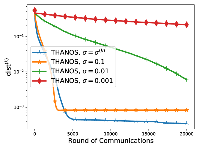
(a) $\mathrm{dist}^{(k)}$

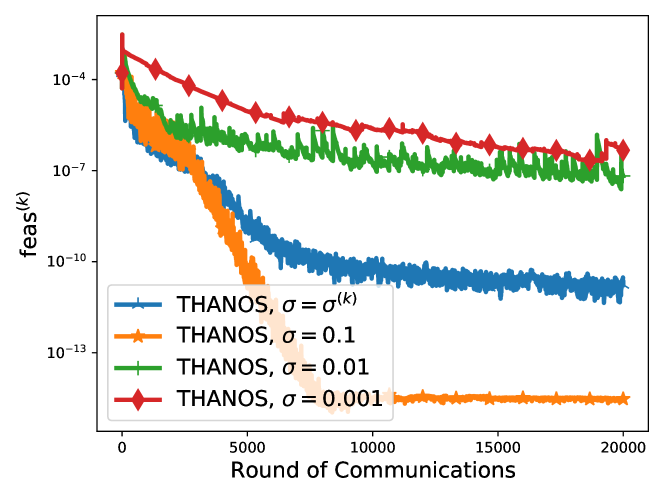
(b) $\mathrm{feas}^{(k)}$

Figure 1: Numerical performance of THANOS for different values of $\sigma$ on sparse PCA problems with $r(X)=\left\|X\right\|_{1}$.

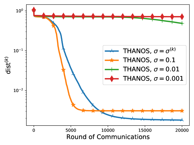
(a) $\mathrm{dist}^{(k)}$

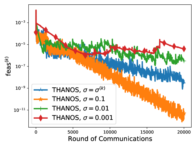
(b) $\mathrm{feas}^{(k)}$

Figure 2: Numerical performance of THANOS for different values of $\sigma$ on sparse PCA problems with $r(X)=\left\|X\right\|_{2,1}$.

Figure 1 and Figure 2 depict the numerical performance of THANOS for two regularizers (9) and (10), respectively. In both figures, we plot $\mathrm{dist}^{(k)}$ and $\mathrm{feas}^{(k)}$ against the iteration count $k$ corresponding to different values of $\sigma$, which are distinguished by colors. We can observe that, the smaller the value of $\sigma$ is, the worse the performance of THANOS becomes. The reason is that the smoothed problem (4) is ill-conditioned for small values of $\sigma$. Moreover, increasing the value of $\sigma$ will give rise to large approximation errors. In order to remedy this dilemma, we propose an updating scheme that gradually reduces the smoothing parameter, that is,

$$\sigma^{(k)}=k^{-1/3},$$

where $\sigma^{(k)}$ is the smoothing parameter at iteration $k$. The above updating scheme has a favorable numerical performance in practice, which is also shown in Figure 1 and Figure 2.

VI CONCLUSIONS

This paper considers a class of decentralized optimization problems over the Stiefel manifold with non-smooth regularizers. There is currently no algorithm in the literature that is capable of solving this problem. To overcome the difficulty of non-smoothness, we use the Moreau envelope to approximate the non-smooth regularizers in the objective function. Then we apply an existing algorithm to solve the obtained smooth proxy of the original problem. The resulting algorithm is called THANOS. We prove that THANOS will return a first-order $\epsilon$-stationary point in at most $\mathcal{O}(\epsilon^{-4})$ iterations. Preliminary numerical results illustrate that THANOS is of great potential.

References

- [1] I. T. Jolliffe, N. T. Trendafilov, and M. Uddin, “A modified principal component technique based on the LASSO,” Journal of Computational and Graphical Statistics, vol. 12, no. 3, pp. 531–547, 2003.
- [2] L. Wang, X. Liu, and Y. Zhang, “A communication-efficient and privacy-aware distributed algorithm for sparse PCA,” arXiv:2106.03320, 2021.
- [3] M. Arjovsky, A. Shah, and Y. Bengio, “Unitary evolution recurrent neural networks,” in International Conference on Machine Learning, pp. 1120–1128, PMLR, 2016.
- [4] L. Huang, X. Liu, B. Lang, A. W. Yu, Y. Wang, and B. Li, “Orthogonal weight normalization: Solution to optimization over multiple dependent Stiefel manifolds in deep neural networks,” in Thirty-Second AAAI Conference on Artificial Intelligence, 2018.
- [5] M. C. Tsakiris and R. Vidal, “Dual principal component pursuit,” Journal of Machine Learning Research, vol. 19, no. 18, pp. 1–49, 2018.
- [6] Z. Zhu, Y. Wang, D. Robinson, D. Naiman, R. Vidal, and M. Tsakiris, “Dual principal component pursuit: Improved analysis and efficient algorithms,” Advances in Neural Information Processing Systems, vol. 31, 2018.
- [7] Z. Zhu, T. Ding, D. Robinson, M. Tsakiris, and R. Vidal, “A linearly convergent method for non-smooth non-convex optimization on the grassmannian with applications to robust subspace and dictionary learning,” Advances in Neural Information Processing Systems, vol. 32, 2019.
- [8] Q. Lu and L. Lian, “Decentralized complete dictionary learning via -norm maximization,” arXiv:2211.03628, 2022.
- [9] P.-A. Absil, R. Mahony, and R. Sepulchre, Optimization algorithms on matrix manifolds. Princeton University Press, 2008.
- [10] S. Chen, A. Garcia, M. Hong, and S. Shahrampour, “Decentralized Riemannian gradient descent on the Stiefel manifold,” in Proceedings of the 38th International Conference on Machine Learning, vol. 139, pp. 1594–1605, PMLR, 2021.
- [11] J. Hu, K. Deng, N. Li, and Q. Li, “Decentralized Riemannian natural gradient methods with Kronecker-product approximations,” arXiv:2303.09611, 2023.
- [12] S. Chen, A. Garcia, M. Hong, and S. Shahrampour, “On the local linear rate of consensus on the Stiefel manifold,” arXiv:2101.09346, 2021.
- [13] L. Wang and X. Liu, “Decentralized optimization over the Stiefel manifold by an approximate augmented Lagrangian function,” IEEE Transactions on Signal Processing, vol. 70, pp. 3029–3041, 2022.
- [14] L. Wang and X. Liu, “A variance-reduced stochastic gradient tracking algorithm for decentralized optimization with orthogonality constraints,” Journal of Industrial and Management Optimization, Early Access, 2023.
- [15] C. Zhang, X. Chen, and S. Ma, “A Riemannian smoothing steepest descent method for non-Lipschitz optimization on submanifolds,” arXiv:2104.04199, 2021.
- [16] Z. Peng, W.-H. Wu, J. Hu, and K.-K. Deng, “Riemannian smoothing gradient type algorithms for nonsmooth optimization problem on manifolds,” arXiv:2212.03526, 2022.
- [17] J. Zhu, J. Huang, L. Yang, and Q. Li, “Smoothing algorithms for nonsmooth and nonconvex minimization over the stiefel manifold,” arXiv:2303.10852, 2023.
- [18] J. Li, S. Ma, and T. Srivastava, “A Riemannian ADMM,” arXiv:2211.02163, 2022.
- [19] X. Li, S. Chen, Z. Deng, Q. Qu, Z. Zhu, and A. Man-Cho So, “Weakly convex optimization over Stiefel manifold using Riemannian subgradient-type methods,” SIAM Journal on Optimization, vol. 31, no. 3, pp. 1605–1634, 2021.
- [20] F. H. Clarke, Optimization and nonsmooth analysis. SIAM, 1990.
- [21] W. H. Yang, L.-H. Zhang, and R. Song, “Optimality conditions for the nonlinear programming problems on Riemannian manifolds,” Pacific Journal of Optimization, vol. 10, no. 2, pp. 415–434, 2014.
- [22] S. Chen, S. Ma, A. Man-Cho So, and T. Zhang, “Proximal gradient method for nonsmooth optimization over the Stiefel manifold,” SIAM Journal on Optimization, vol. 30, no. 1, pp. 210–239, 2020.
- [23] K. Yuan, Q. Ling, and W. Yin, “On the convergence of decentralized gradient descent,” SIAM Journal on Optimization, vol. 26, no. 3, pp. 1835–1854, 2016.
- [24] W. Shi, Q. Ling, G. Wu, and W. Yin, “EXTRA: An exact first-order algorithm for decentralized consensus optimization,” SIAM Journal on Optimization, vol. 25, no. 2, pp. 944–966, 2015.
- [25] A. Nedić, A. Olshevsky, and M. G. Rabbat, “Network topology and communication-computation tradeoffs in decentralized optimization,” Proceedings of the IEEE, vol. 106, no. 5, pp. 953–976, 2018.
- [26] S. U. Pillai, T. Suel, and S. Cha, “The Perron-Frobenius theorem: some of its applications,” IEEE Signal Processing Magazine, vol. 22, no. 2, pp. 62–75, 2005.
- [27] J.-J. Moreau, “Proximité et dualité dans un espace hilbertien,” Bulletin de la Société Mathématique de France, vol. 93, pp. 273–299, 1965.
- [28] R. T. Rockafellar and R. J.-B. Wets, Variational analysis, vol. 317. Springer Science & Business Media, 2009.
- [29] X. Chen, “Smoothing methods for nonsmooth, nonconvex minimization,” Mathematical Programming, vol. 134, pp. 71–99, 2012.
- [30] A. Böhm and S. J. Wright, “Variable smoothing for weakly convex composite functions,” Journal of Optimization Theory and Applications, vol. 188, pp. 628–649, 2021.
- [31] L. Wang, B. Gao, and X. Liu, “Multipliers correction methods for optimization problems over the Stiefel manifold,” CSIAM Transactions on Applied Mathematics, vol. 2, no. 3, pp. 508–531, 2021.
- [32] W. Bian and X. Chen, “A smoothing proximal gradient algorithm for nonsmooth convex regression with cardinality penalty,” SIAM Journal on Numerical Analysis, vol. 58, no. 1, pp. 858–883, 2020.
- [33] W. Liu, X. Liu, and X. Chen, “Linearly constrained nonsmooth optimization for training autoencoders,” SIAM Journal on Optimization, vol. 32, no. 3, pp. 1931–1957, 2022.
- [34] L. Wang, X. Liu, and Y. Zhang, “Seeking consensus on subspaces in federated principal component analysis,” arXiv:2012.03461, 2020.
- [35] N. Xiao, X. Liu, and Y.-X. Yuan, “Exact penalty function for norm minimization over the Stiefel manifold,” SIAM Journal on Optimization, vol. 31, no. 4, pp. 3097–3126, 2021.
- [36] N. Xiao, X. Liu, and Y.-X. Yuan, “A penalty-free infeasible approach for a class of nonsmooth optimization problems over the Stiefel manifold,” arXiv:2103.03514, 2021.