Criteria for entropic curvature
on graph spaces

Abstract.

This paper presents local criteria for lower bounds on entropic curvature of graph spaces along Schrödinger bridges at zero temperature, according to the definition given by the second named author in [47], in the continuity of the work by C. Léonard [31] inspired by the Lott-Sturm-Villani theory.

A graph space is defined as a quadruple $({\mathcal{X}},d,L,m)$ where ${\mathcal{X}}$ is the set of vertices of a graph, $d$ is the combinatorial distance of the graph and $m$ is a reversible reference measure with respect to a generator $L$ of a Markov semi-group. The criteria are given by local optimization problems on balls of radius two, depending only on the generator $L$ and on the geometric discrete structure of these balls. General tensorization properties of the criteria are presented for the study of the Cartesian product of graphs.

This approach is robust since it applies to a very wide range of graph spaces and also for any measure $m$, including measures with interaction potential like Ising models, as example the so-called Sherrington-Kirkpatrick model from the spin glass theory (see Section 6). We also introduce very large classes of graphs for which the local criteria give non-negative entropic curvature for the uniform measure. A Bonnet-Myers type of theorem also ensures that any graph with positive entropic curvature is finite.

On any graph space $({\mathcal{X}},d,L,m)$ with $m({\mathcal{X}})<\infty$, positive entropic curvature provides transport-entropy inequalities with so-called weak optimal transport costs, as well as Poincaré or modified logarithmic-Sobolev inequalities for the renormalized probability measure $\mu=m/m({\mathcal{X}})$. These functional inequalities are well known to be related to refined concentration properties of the measure $\mu$, speed of convergence of semi-groups to the measure $\mu$ or bounds on its mixing time. For certain specific graph spaces, the local criteria are optimal and imply sharp functional inequalities.

We also present examples of graphs with negative curvature. Some comparisons of our results with other notions of curvature are established, such as Bakry-Emery curvature conditions [14, 15], Ollivier or Lin-Lu-Yau’s curvature [42, 32].

1. Introduction

Let us present the framework of this research, in keeping with the seminal papers [31, 47]. Let ${\mathcal{X}}$ be the set of vertices of a connected undirected graph $G=({\mathcal{X}},E)$ where $E$ denotes the set of edges, without multiple edges and without loops. Two vertices $x$ and $y$ are neighbours if $\{x,y\}$ is an edge of $E$, we write $x\sim y$ in this case. Let $d$ denote the combinatorial graph distance, so that $d(x,y)=1$ if and only if $x\sim y$. The graph $G$ is supposed to be locally finite, that is, the vertex degree $\text{deg}(x):=\sum_{y\sim x}1$ of any $x\in\mathcal{X}$ is finite. The maximal degree of the graph is denoted by $\Delta(G):=\sup_{x\in\mathcal{X}}\text{deg}(x)\in{\mathbb{N}}\cup\{+\infty\}$. A discrete geodesic path $\alpha$ joining two vertices $x$ and $y$ is a sequence of neighbours of minimal size $d=d(x,y)$: $\alpha=(z_{0},\ldots,z_{d})$ with $z_{0}=x$ and $z_{d}=y$ and for any $i\in[d]:=\{1,\cdots,d\}$, $\{z_{i-1},z_{i}\}\in E$. In the sequel, $z\in\alpha$ means that there exists $i\in\{0,\ldots,d\}$ such that $z=z_{i}$, and $(z,w)\in\alpha$ means that there exists $0\leq i<j\leq\ell$ such that $z=z_{i}$ and $w=z_{j}$. Let $G(x,y)$ be the set of all geodesic paths joining $x$ to $y$, and let $[x,y]$ be the set of all vertices that belong to a geodesic from $x$ to $y$,

$$[x,y]:=\big{\{}z\in{\mathcal{X}}\,\big{|}\,z\in\alpha,\alpha\in G(x,y)\big{\}},$$

$]x,y[:=[x,y]\setminus\{x,y\}$ and $[x,y[:=[x,y]\setminus\{y\}$. More generally, given two subsets $A$ and $B$ of ${\mathcal{X}}$, one defines

$$[A,B]:=\bigcup_{x\in A,y\in B}[x,y]\quad\mbox{and}\quad]A,B[:=\bigcup_{x\in A,y\in B}]x,y[.$$

The set ${\mathcal{X}}$ is endowed with the $\sigma$-algebra generated by singletons. Let $\mathcal{P}({\mathcal{X}})$ denote the set of probabilities on ${\mathcal{X}}$, and $\mathcal{P}_{b}({\mathcal{X}})$ the subset of probabilities with bounded support. The subset of probability measures $\mu$ satisfying $\int d(x_{0},y)d\mu(y)<\infty$ for some $x_{0}\in{\mathcal{X}}$, denoted by ${\mathcal{P}}_{1}({\mathcal{X}})$, can be endowed with the $W_{1}$-Wasserstein distance defined as usual by

(1) $$W_{1}(\nu_{0},\nu_{1}):=\inf_{\pi\in\Pi(\nu_{0},\nu_{1})}\iint d(x,y)\,d\pi(x,y),\qquad\nu_{0},\nu_{1}\in{\mathcal{P}}_{1}({\mathcal{X}}),$$

where $\Pi(\nu_{0},\nu_{1})$ is the set of probability measures on the product space ${\mathcal{X}}\times{\mathcal{X}}$ with first marginal $\nu_{0}$ and second marginal $\nu_{1}$. We call $W_{1}$-optimal coupling of $\nu_{0}$ and $\nu_{1}$ any coupling $\pi\in\Pi(\nu_{0},\nu_{1})$ that achieves the infimum in (1). For any non negative measure $M$ on a measurable space $\mathcal{Y}$, $\mathrm{supp}(M)$ denotes the support of this measure. For further use, note that any measure $\pi\in\Pi(\nu_{0},\nu_{1})$ admits the two following decompositions : for any $(x,y)\in\mathrm{supp}(\pi)$,

$$\pi(x,y)=\nu_{0}(x)\,{\pi}_{{}_{\rightarrow}}(y|x)=\nu_{1}(y)\,{\pi}_{{}_{\leftarrow}}(x|y),$$

defining thus two Markov kernels ${\pi}_{{}_{\rightarrow}}$ and ${\pi}_{{}_{\leftarrow}}$.

On a discrete space ${\mathcal{X}}$, recall that any generator $L$ acting on functions from ${\mathcal{X}}$ to ${\mathbb{R}}$ is entirely given by the jump rates from $x\in{\mathcal{X}}$ to $y\in{\mathcal{X}}$ denoted by $L(x,y)$, $L(x,y):=L\delta_{y}(x)$ with $\delta_{y}(y)=1$ and $\delta_{y}(z)=0$ for $z\neq y$.

In this paper, we call graph space any locally finite graph $G=({\mathcal{X}},E)$ as above endowed with a reference measure $m$ on ${\mathcal{X}}$ and a generator $L$ satisfying the following two conditions :

• The measure $m$ is reversible with respect to $L$, $m(x)L(x,y)=m(y)L(y,x)$ for any $x,y\in{\mathcal{X}}$.

• For any $x,y\in{\mathcal{X}}$, one has

  (2) $$L(x,y)>0\quad\mbox{ if and only if }\quad x\sim y,$$

  (and $L(x,x):=-\sum_{y\in{\mathcal{X}},y\neq x}L(x,y)$).

For simplicity, one also denotes $G=({\mathcal{X}},d,L,m)$ in that case.

In this paper, given $m$, two specific generic generators $L_{1}$ and $L_{2}$ will be considered at different places defined by, for all $x\neq y$

(3) $$L_{1}(x,y)=\Big{(}\frac{m(x)}{m(y)}\Big{)}^{1/2}dir0{o}_{x\sim y}\quad\mbox{and}\quad L_{2}(x,y)=\frac{1}{2}\Big{(}1+\frac{m(x)}{m(y)}\Big{)}dir0{o}_{x\sim y}.$$

Note that for the counting measure on ${\mathcal{X}}$, denoted by $m_{0}$ in this paper, these two generators are the same and one denotes in that case $L_{0}:=L_{1}=L_{2}$.

By definition, for any $x,y\in{\mathcal{X}}$ and $k\in{\mathbb{N}}^{*}$, one denotes

$$L^{k}(x,y):=\sum_{z_{1},z_{2},\ldots,z_{k-1}\in{\mathcal{X}}}L(x,z_{1})L(z_{1},z_{2})\cdots L(z_{k-1},y).$$

The property (2) ensures that for any $x,y\in{\mathcal{X}}$,

$$L^{d(x,y)}(x,y)=\sum_{\alpha\in G(x,y)}L(\alpha),\quad\mbox{where}\quad L(\alpha):=L(z_{0},z_{1})\cdots L(z_{d(x,y)-1},z_{d(x,y)}),$$

for any $\alpha=(z_{0},z_{1},\ldots,z_{d(x,y)})\in G(x,y)$.

As defined in [47], given $\nu_{0},\nu_{1}\in\mathcal{P}_{b}({\mathcal{X}})$, a Schrödinger bridge at zero temperature, denoted by $(\widehat{\nu}_{t})_{t\in[0,1]}$ in the present paper, is a particular $W_{1}$ constant speed geodesic between $\nu_{0}$ and $\nu_{1}$ on ${\mathcal{P}}({\mathcal{X}})$, namely, $\widehat{\nu}_{0}=\nu_{0}$, $\widehat{\nu}_{1}=\nu_{1}$, and for any $0\leq s\leq t\leq 1$,

$$W_{1}\big{(}\widehat{\nu}_{t},\widehat{\nu}_{s}\big{)}=(t-s)W_{1}(\nu_{0},\nu_{1}).$$

Such a path is obtained from a mixture of Schrödinger bridges, by a slowing down procedure as a temperature term goes to zero due to C. Léonard [30, Theorem 2.1] (see also [47]). These geodesic paths are mixture of $W_{1}$-constant speed geodesics $\nu_{t}^{x,y}$ between the Dirac measures $\delta_{x}$ at $x\in\mathrm{supp}(\nu_{0})$ and $\delta_{y}$ at $y\in\mathrm{supp}(\nu_{1})$, according to a coupling $\widehat{\pi}\in\Pi(\nu_{0},\nu_{1})$. Observe that given bounded marginals $\nu_{0}$ and $\nu_{1}$, the Léonard slowing down procedure selects a single coupling $\widehat{\pi}\in\Pi(\nu_{0},\nu_{1})$ if some conditions are satisfied on the underlying space [30, Result 0.3]. The main property of $\widehat{\pi}$ is to be a $W_{1}$-optimal coupling. As explained in [47], the structure of Schrödinger bridges at zero temperature that we also consider in this paper is the following: for any $z\in{\mathcal{X}}$

(4) $$\widehat{\nu}_{t}(z):=\sum_{x,y\in{\mathcal{X}}}\nu_{t}^{x,y}(z)\,\widehat{\pi}(x,y),$$

with for any $x,y\in{\mathcal{X}}$,

(5) $$\nu_{t}^{x,y}(z):=dir0{o}_{[x,y]}(z)\,r(x,z,z,y)\,{\rho}_{t}^{d(x,y)}(d(x,z)),$$

where for $x,z,v,y\in{\mathcal{X}}$,

(6) $$r(x,z,v,y):=\frac{L^{d(x,z)}(x,z)L^{d(v,y)}(v,y)}{L^{d(x,y)}(x,y)},$$

and ${\rho}_{t}^{d}$ denotes the binomial law with parameter $t\in[0,1]$, $d\in{\mathbb{N}}$ :

$${\rho}_{t}^{d}(k):=\binom{d}{k}\,t^{k}(1-t)^{d-k},\quad k\in\{0,\ldots,d\},$$

with the binomial coefficient $\binom{d}{k}:=\frac{d!}{k!(d-k)!}$. All along the paper one omits the dependence in $\nu_{0}$ and $\nu_{1}$ of $(\widehat{\nu}_{t})_{t\in[0,1]}$ and $\widehat{\pi}$ to lighten the notations.

After the Lott-Sturm-Villani theory of curvature on Riemannian manifold or more generally on geodesic spaces [36, 49, 53], it has been a challenging problem to define good notions of curvature in discrete spaces. In the paper [47], by analogy of the definition of entropic curvature due to Lott-Sturm-Villani, this property is expressed on a graph space $({\mathcal{X}},d,L,m)$ in terms of a convexity property of the relative entropy along Schrödinger bridges at zero temperature. By definition, the relative entropy of a probability measure $q$ on a measurable space $\mathcal{Y}$ with respect to a probability measure $r\in{\mathcal{P}}(\mathcal{Y})$ is given by

$${\mathcal{H}}(q|r):=\int_{\mathcal{Y}}\log(dq/dr)\,dq\qquad\in[0,\infty],$$

if $q$ is absolutely continuous with respect to $r$ and ${\mathcal{H}}(q|r):=+\infty$ otherwise. As recalled in [47], this definition extends to $\sigma$-finite non-negative measures $r$ adding weak conditions on $q\in{\mathcal{P}}(\mathcal{Y})$, and in that case ${\mathcal{H}}(q|r)\in(-\infty,\infty]$.

Definition 1.

[47] On the graph space $({\mathcal{X}},d,m,L)$, one says that the relative entropy is $C$-displa-cement convex where $C=(C_{t})_{t\in[0,1]}$, if for any probability measures $\nu_{0},\nu_{1}\in\mathcal{P}_{b}({\mathcal{X}})$, there exists a Schrödinger bridge at zero temperature $(\widehat{\nu}_{t})_{t\in[0,1]}$ whose structure is given by (4), and such that for any $t\in(0,1)$,

(7) $${\mathcal{H}}(\widehat{\nu}_{t}|m)\leq(1-t){\mathcal{H}}(\nu_{0}|m)+t\,{\mathcal{H}}(\nu_{1}|m)-\frac{t(1-t)}{2}C_{t}(\widehat{\pi}),$$

where $\widehat{\pi}$ is the $W_{1}$-optimal coupling between $\nu_{0}$ and $\nu_{1}$ that appears in (4).

Observe that such a property on graphs has been first proposed by M. Erbar and J. Maas [37, 19, 20] where the cost $C_{t}(\widehat{\pi})$ is replaced by $\kappa{\mathcal{W}}_{2}^{2}(\nu_{0},\nu_{1})$, with $\kappa\in{\mathbb{R}}$ and ${\mathcal{W}}_{2}$ an abstract Wasserstein distance on ${\mathcal{P}}({\mathcal{X}})$. In that framework, Schrödinger bridges at zero temperature are also replaced by a ${\mathcal{W}}_{2}$-geodesic, and the best constant $\kappa$ represents the so-called entropic curvature of the space. Actually, the distance ${\mathcal{W}}_{2}$ is defined using a discrete type of Benamou-Brenier formula in order to provide a Riemannian structure for the probability space ${\mathcal{P}}({\mathcal{X}})$. This distance ${\mathcal{W}}_{2}$ is greater than $\sqrt{2}W_{1}$, however ${\mathcal{W}}_{2}$ can not be expressed as a minimum of a cost among transference plans $\pi$ as in the definition (1) of $W_{1}$. As we will see further in this paper, one of the main advantages of the Schrödinger method initiated in [47], is to capture such types of costs and also to be able to introduce new interesting ones. These transport costs, also called weak optimal transport costs, appear in the literature to describe refined concentration phenomena in discrete spaces (see [23]).

Contents

1. 1 Introduction
2. 2 Main results for any graph space
3. 3 Refined results for structured graph spaces
4. 4 Perturbation results
   1. 4.1 Perturbation with a potential
   2. 4.2 Restriction to convex subsets
5. 5 Tensorization properties
6. 6 Entropic curvature on the discrete hypercube and on the lattice ${\mathbb{Z}}^{n}$ equipped with measures with interaction potential
   1. 6.1 The discrete hypercube and the Ising model
   2. 6.2 The lattice ${\mathbb{Z}}^{n}$
7. 7 Non positively curved graphs
8. 8 Geometric conditions for positive entropic curvature via the Motzkin-Strauss Theorem.
9. 9 Few comparisons with other notions of curvature.
10. 10 Appendix A
11. 11 Appendix B
    1. 11.1 Proofs of Theorem 1, Theorem 2 and Theorem 7
    2. 11.2 Proofs of Theorem 4, Theorem 6, Theorem 5, Theorem 8 and Theorem 11
       1. 11.2.1 Proofs of Lemma 1, Lemma 2 and Lemma 3
    3. 11.3 Proof of Proposition 6 and Proposition 7

2. Main results for any graph space

In this part, we focus on the convexity property (7) for very general graph spaces, which means without a particular geometric structure. One of the main result of this paper, Theorem 1 below, introduces a uniform local criteria on the graph space $({\mathcal{X}},d,m,L)$ under which the cost $C_{t}(\widehat{\pi})$ can be replaced by $\kappa\,T_{2}(\widehat{\pi})$ with

$$T_{2}(\widehat{\pi}):=\iint d(x,y)(d(x,y)-1)\,d{\widehat{\pi}}(x,y).$$

By definition, we call entropic curvature of the graph space $({\mathcal{X}},d,m,L)$ denoted by $\kappa$ the supremum of $k\in{\mathbb{R}}$ such that the $C$-displacement convexity property $\eqref{deplacebis}$ holds with $C_{t}=k\,T_{2}$. Observe that if $\kappa=+\infty$ then $\eqref{deplacebis}$ ensures that $T_{2}(\widehat{\pi})=0$ since $H(\widehat{\nu}_{t}|m)<+\infty$ for any $\nu_{0},\nu_{1}\in{\mathcal{P}}_{b}({\mathcal{X}})$. As a convention $\kappa T_{2}(\widehat{\pi})=0$ if $\kappa=+\infty$. When $\kappa>0$ (respectively $\kappa\geq 0$), one says that the space $({\mathcal{X}},d,m,L)$ has positive entropic curvature (respectively non-negative entropic curvature). More generally, given a family of cost functions $c=(c_{t})_{t\in(0,1)}$, $c_{t}:{\mathbb{N}}\to{\mathbb{R}}$, we call $T_{c}$-entropic curvature of the graph space $({\mathcal{X}},d,m,L)$ the best constant $\kappa_{c}\in{\mathbb{R}}\cup\{+\infty\}$ such that the $C$-displacement convexity property $\eqref{deplacebis}$ holds for all $t\in(0,1)$ with $C_{t}=\kappa_{c}\,T_{c_{t}}$ with

$$T_{c_{t}}(\widehat{\pi}):=\iint c_{t}(d(x,y))\,d{\widehat{\pi}}(x,y).$$

Similarly, let us also introduce a definition of ${\widetilde{T}}$-entropic curvature as the best constant $\widetilde{\kappa}\in{\mathbb{R}}$ such that (7) holds with $C_{t}=\widetilde{\kappa}\,\widetilde{T}$ and $\widetilde{T}=\max\big{(}\widetilde{T}_{{}_{\rightarrow}},\widetilde{T}_{{}_{\leftarrow}}\big{)},$ where

$$\widetilde{T}_{{}_{\rightarrow}}(\widehat{\pi}):=\int\left(\int d(x,w)\,d{\widehat{\pi}}_{{}_{\rightarrow}}(w|x)\right)^{2}d\nu_{0}(x)\quad\mbox{and}\quad\widetilde{T}_{{}_{\leftarrow}}(\widehat{\pi}):=\int\left(\int d(w,y)\,d{\widehat{\pi}}_{{}_{\leftarrow}}(w|y)\right)^{2}d\nu_{1}(y).$$

Let us note that as soon as ${\mathcal{X}}$ is not reduced to a singleton, there always exist $\nu_{0}$ and $\nu_{1}\in{\mathcal{P}}_{b}({\mathcal{X}})$ such that $\widetilde{T}_{{}_{\rightarrow}}(\widehat{\pi})>0$ or $\widetilde{T}_{{}_{\leftarrow}}(\widehat{\pi})>0$ in such a way that $\widetilde{\kappa}<+\infty$.

Analogously, we also call $W_{1}$-entropic curvature of the graph space $({\mathcal{X}},d,m,L)$ the best constant $\kappa_{1}\in{\mathbb{R}}$ such that (7) holds with $C_{t}=\kappa_{1}\,W_{1}^{2}.$ By the Cauchy-Schwarz inequality and since $\widehat{\pi}$ is a $W_{1}$-optimal coupling, one has $\widetilde{T}_{{}_{\rightarrow}}(\widehat{\pi})\geq W_{1}^{2}(\nu_{0},\nu_{1})$ and therefore, if $\widetilde{\kappa}\geq 0$ then one has

$$\kappa_{1}\geq\widetilde{\kappa}.$$

Further in this introduction, one gives examples of graphs for which this inequality is strict. A second main result of this paper, Theorem 2 below, presents refined criteria for non-negative $W_{1}$-entropic curvature, non-negative ${\widetilde{T}}$-entropic curvature and also some non-negative $T_{c}$-entropic curvature for a specific family of costs $c=(c_{t})_{t\in(0,1)}$, related to the cost $T_{2}$.

Let us now introduce the key quantities that allow to define the criteria of Theorem 1 and Theorem 2. For $z\in{\mathcal{X}}$, let $B_{1}(z):=\{w\in{\mathcal{X}}\,|\,d(z,w)\leq 1\}$ denotes the ball of radius one centered at $z$, and for $k=1$ or $k=2$ let the combinatorial sphere $S_{k}(z)$ denotes the set of vertices at distance $k$ from $z$

$$S_{k}(z):=\Big{\{}w\in{\mathcal{X}}\,\Big{|}\,d(z,w)=k\Big{\}}.$$

Given a vertex $z\in{\mathcal{X}}$ and a subset $W\subset S_{2}(z)$, the next non-negative key quantity will be used for local lower bound on entropic curvature

(8) $$K_{L}(z,W):=\sup\Biggl{\{}\sum_{z^{\prime\prime}\in W}L^{2}(z,z^{\prime\prime})\prod_{z^{\prime}\in]z,z^{\prime\prime}[}\left(\frac{\alpha(z^{\prime})}{L(z,z^{\prime})}\right)^{2\ell(z,z^{\prime},z^{\prime\prime})}\Biggl{|}\,{\alpha}:]z,W[\to\mathbb{R}_{+},\sum_{v\in]z,W[}\alpha(v)=1\Biggr{\}},$$

with $\ell(z,z^{\prime},z^{\prime\prime}):=\frac{L(z,z^{\prime})L(z^{\prime},z^{\prime\prime})}{L^{2}(z,z^{\prime\prime})}$. To simplify the notations, one omits the dependence in $L$ and notices $K=K_{L}$ when there is no possible confusions. In this definition as in the all paper, we use the convention that a sum indexed by an empty set is $0$. Therefore, $K(z,W)=0$ holds if and only if $W=\emptyset$. One may easily check that given $z$ the quantity $K(z,W)$ is increasing in $W$. Namely, for $W\subset W^{\prime}\subset S_{2}(z)$, it holds

(9) $$K(z,W)\leq K(z,W^{\prime})\leq K\big{(}z,S_{2}(z)\big{)}.$$

For more comprehension about this quantity, consider the special case where $m=m_{0}$ is the counting measure and $L=L_{0}$. Let $|A|$ denote the cardinal of any finite set $A\subset{\mathcal{X}}$. Then (8) becomes

(10) $$K_{0}(z,W):=K_{L_{0}}(z,W)=\sup_{\alpha}\Biggl{\{}\sum_{z^{\prime\prime}\in W}\big{|}]z,z^{\prime\prime}[\big{|}\Big{(}\prod_{z^{\prime}\in]z,z^{\prime\prime}[}{\alpha(z^{\prime})}\Big{)}^{\frac{2}{|]z,z^{\prime\prime}[|}}\Biggr{\}},$$

where the supremum runs over all $\alpha:]z,W[\to\mathbb{R}_{+}$ such that $\sum_{v\in]z,W[}\alpha(v)=1$. Note that given a vertex $z\in{\mathcal{X}}$, the existence of edges between vertices exclusively within $S_{1}(z)$ or $S_{2}(z)$ respectively does not change the value of $K\big{(}z,S_{2}(z)\big{)}$.

In order to introduce a first general criterion that provides lower bounds on entropic curvature, one needs to recall few notions dealing with optimal transport. According to the theory of optimal transport, the support of any $W_{1}$-optimal coupling is $d$-cyclically monotone (see [53, Theorem 5.10]). Recall that by definition, a subset $S\subset{\mathcal{X}}\times{\mathcal{X}}$ is $d$-cyclically monotone if for any family $(x_{1},y_{1}),\ldots,(x_{N},y_{N})$ of points in $S$,

$$\sum_{i=1}^{N}d(x_{i},y_{i})\leq\sum_{i=1}^{N}d(x_{i},y_{i+1}),$$

with the convention $y_{N+1}=y_{1}$. As a trivial example, for any $z\in{\mathcal{X}}$ and $V\subset{\mathcal{X}}$, the set $\{x\}\times V$ is a $d$-cyclically monotone subset of ${\mathcal{X}}\times{\mathcal{X}}$. Given such a subset $S$, one defines

$$Z(S):=\Big{\{}z\in{\mathcal{X}}\,\Big{|}\,\exists(x,y)\in S,z\in[x,y]\Big{\}},$$

$$C_{{}_{\rightarrow}}(S):=\Big{\{}(z,w)\in{\mathcal{X}}\times{\mathcal{X}}\,\Big{|}\,z\neq w,\exists(x,y)\in S,(z,w)\in[x,y]\Big{\}},$$

$$C_{{}_{\leftarrow}}(S):=\Big{\{}(z,w)\in{\mathcal{X}}\times{\mathcal{X}}\,\Big{|}(w,z)\in C_{{}_{\rightarrow}}(S)\Big{\}},$$

and for $z\in Z(S)$,

$$V^{S}_{{}_{\rightarrow}}(z):=\Big{\{}z^{\prime}\in S_{1}(z)\,\Big{|}\,(z,z^{\prime})\in C_{{}_{\rightarrow}}(S)\Big{\}},\quad\quad V^{S}_{{}_{\leftarrow}}(z):=\Big{\{}z^{\prime}\in S_{1}(z)\,\Big{|}\,(z,z^{\prime})\in C_{{}_{\leftarrow}}(S)\Big{\}}.$$

Setting $\ell(z,z^{\prime},z^{\prime\prime}):=\frac{L(z,z^{\prime})L(z^{\prime},z^{\prime\prime})}{L^{2}(z,z^{\prime\prime})}$ and $\mathcal{L}^{2}(z,z^{\prime\prime}):=\sqrt{L^{2}(z,z^{\prime\prime})L^{2}(z^{\prime\prime},z)}$, let

$$K_{L}(S)=K(S):=\sup_{\alpha,\beta}\Biggl{\{}\sum_{(z,z^{\prime\prime})\in C_{{}_{\rightarrow}}(S),d(z,z^{\prime\prime})=2}\mathcal{L}^{2}(z,z^{\prime\prime})\prod_{z^{\prime}\in]z,z^{\prime\prime}[}\left(\frac{\beta(z,z^{\prime})}{L(z,z^{\prime})}\frac{\alpha(z^{\prime\prime},z^{\prime})}{L(z^{\prime\prime},z^{\prime})}\right)^{\ell(z,z^{\prime},z^{\prime\prime})}\Biggl{\}},$$

where the supremum runs over all non negative functions $\alpha$ and $\beta$ on ${\mathcal{X}}\times{\mathcal{X}}$ satisfying

$$\sum_{z\in Z(S)}\Big{(}\sum_{z^{\prime}\in V^{S}_{{}_{\rightarrow}}(z)}\beta(z,z^{\prime})\Big{)}^{2}=1\quad\mbox{and}\quad\sum_{z^{\prime\prime}\in Z(S)}\Big{(}\sum_{z^{\prime}\in V^{S}_{{}_{\leftarrow}}(z^{\prime\prime})}\alpha(z^{\prime\prime},z^{\prime})\Big{)}^{2}=1.$$

Observe that if there exists $(x,y)\in S$ such that $d(x,y)\geq 2$ then $(x,y)\in\big{\{}(z,z^{\prime\prime})\in C_{{}_{\rightarrow}}(S),d(z,z^{\prime\prime})=2\big{\}}\neq\emptyset$ and therefore $K(S)>0$.

For the uniform measure $m_{0}$ on ${\mathcal{X}}$ with $L=L_{0}$, one has

(11) $$K_{0}(S):=K_{L_{0}}(S)=\sup_{\alpha,\beta}\Biggl{\{}\sum_{(z,z^{\prime\prime})\in C_{{}_{\rightarrow}}(S),d(z,z^{\prime\prime})=2}\big{|}]z,z^{\prime\prime}[\big{|}\prod_{z^{\prime}\in]z,z^{\prime\prime}[}\big{(}{\beta(z,z^{\prime})}{\alpha(z^{\prime\prime},z^{\prime})}\big{)}^{\frac{1}{|]z,z^{\prime\prime}[|}}\Biggl{\}}$$

The quantity $K_{L}(S)$ is upper-bounded by $\sup_{z\in{\mathcal{X}}}K(z,S_{2}(z))$. Indeed, the reversibility property implies $\ell(z,z^{\prime},z^{\prime\prime})=\ell(z^{\prime\prime},z^{\prime},z)$ and one has $\sum_{z^{\prime}\in]z,z^{\prime\prime}[}\ell(z,z^{\prime},z^{\prime\prime})=1$. Therefore by setting

$$\mathbb{V}^{S}_{{}_{\rightarrow}}(z):=\Big{\{}z^{\prime\prime}\in S_{2}(z)\,\Big{|}\,(z,z^{\prime\prime})\in C_{{}_{\rightarrow}}(S)\Big{\}}\quad\mbox{and}\quad\mathbb{V}^{S}_{{}_{\leftarrow}}(z):=\Big{\{}z^{\prime\prime}\in S_{2}(z)\,\Big{|}\,(z,z^{\prime\prime})\in C_{{}_{\leftarrow}}(S)\Big{\}},$$

for $z\in Z(S)$, the Cauchy-Schwarz inequality provides

$$K(S)^{2} \leq\sup_{\beta}\Biggl{\{}\sum_{z\in Z(S)}\sum_{z^{\prime\prime}\in{\mathbb{V}}^{S}_{{}_{\rightarrow}}(z)}L^{2}(z,z^{\prime\prime})\prod_{z^{\prime}\in]z,z^{\prime\prime}[}\left(\frac{\beta(z,z^{\prime})}{L(z,z^{\prime})}\right)^{2\ell(z,z^{\prime},z^{\prime\prime})}\Biggl{\}}$$

$$\qquad\qquad\qquad\cdot\sup_{\alpha}\Biggl{\{}\sum_{z^{\prime\prime}\in Z(S)}\sum_{z\in{\mathbb{V}}^{S}_{{}_{\leftarrow}}(z^{\prime\prime})}L^{2}(z^{\prime\prime},z)\prod_{z^{\prime}\in]z,z^{\prime\prime}[}\left(\frac{\alpha(z^{\prime\prime},z^{\prime})}{L(z^{\prime\prime},z^{\prime})}\right)^{2\ell(z^{\prime\prime},z^{\prime},z)}\Biggl{\}}$$

(12) $$\leq\sup_{z\in Z(S)}K\big{(}z,{\mathbb{V}}^{S}_{{}_{\rightarrow}}(z)\big{)}\,\sup_{z^{\prime\prime}\in Z(S)}K\big{(}z^{\prime\prime},{\mathbb{V}}^{S}_{{}_{\leftarrow}}(z^{\prime\prime})\big{)}\leq\sup_{z\in{\mathcal{X}}}K(z,S_{2}(z))^{2},$$

where the last inequality is a consequence of the monotonicity property (9).

Here is the main result of this paper that will be analyzed for a variety of graph spaces in this work. Its proof is given in Appendix B.

Theorem 1.

Let $({\mathcal{X}},d,m,L)$ be a graph space. Let

$$K=K_{L}:=\sup_{S}K_{L}(S),$$

where the supremum is over all $d$-cyclically monotone subsets of ${\mathcal{X}}\times{\mathcal{X}}$. Then the entropic curvature $\kappa$ of the space $({\mathcal{X}},d,m,L)$ is bounded from below by $r=r^{L}:=-2\log K$ if $K>0$, and $\kappa=+\infty$ if $K=0$.

Comments:

1. Observe that $K=0$ if and only if $G=({\mathcal{X}},E)$ is a complete graph. Indeed, if $K=0$ then for any singleton $\{(x,y)\}$ of ${\mathcal{X}}\times{\mathcal{X}}$, one has $K(\{(x,y)\})=0$ and therefore $d(x,y)\leq 1$.

2. For most of graphs, computing $K$ is not easy since we need first to characterise the set of $d$-cyclically monotone subsets. However one may use the estimate given by inequality (2) which is more tractable. More precisely, for $z\in{\mathcal{X}}$, let us define

   (13) $$r(z)=r^{L}(z):=-2\log K_{L}\big{(}z,S_{2}(z)\big{)}.$$

   Then, according to (2), Theorem 1 ensures that $\kappa\geq r\geq\inf_{z\in{\mathcal{X}}}r(z)$. Actually, the quantity $r(z)$ can be interpreted as a local lower bound on entropic curvature at vertex $z$. This quantity only depends on the value of the jump rates on the ball of radius 2 centered at $z$. If the graph space is equipped with the counting measure ($m=m_{0}$ and $L=L_{0}$), then $r_{0}(z):=r^{L_{0}}(z)$ only depends on the structure of the ball $B_{2}(z)$. Therefore a lower bound on this local quantity can be interpreted as a geometric property of the balls of radius 2. The lower bound on entropic curvature $\inf_{z\in{\mathcal{X}}}r(z)$ is really useful since it can be estimated on a wide range of graphs. Morevover, as shown in section 6, this lower bound provides new results for complex measures with interaction potentials, like for Ising models. Therefore it should give promissing results for many other specific graph spaces which are not considered in this paper.

3. For more comprehension, let us present a simple necessary condition for $r>0$, as $m=m_{0}$ is the counting measure. According to (11), if for some $z_{0}\in{\mathcal{X}}$, there exists $z^{\prime\prime}_{0}\in S_{2}(z_{0})$ such that $\big{|}]z_{0},z^{\prime\prime}_{0}[\big{|}=1$, or equivalently $]z_{0},z^{\prime\prime}_{0}[=\{z^{\prime}_{0}\}$, then for $S_{0}:=\{(z_{0},z^{\prime\prime}_{0})\}$ one has $K(S_{0})=1$ and therefore $r\leq 0$. As a consequence, if the criteria of Theorem 1 provides positive entropic curvature for the space $({\mathcal{X}},d,m_{0},L_{0})$, then there is at least 2 midpoints between any two vertices at distance 2.

Theorem 1 ensures that if $K\leq 1$ then the graph space $({\mathcal{X}},d,m,L)$ has non-negative entropic curvature, i.e. $\kappa\geq 0$. Section 7 and section 8 are devoted to the study of the upper bound $\sup_{z\in{\mathcal{X}}}K_{0}(z,S_{2}(z))\geq K$ in order to give necessary or sufficient conditions for non-negative or positive entropic curvature for the space $({\mathcal{X}},d,m_{0},L_{0})$. The next result states that $K\leq 1$ also implies non-negative $\widetilde{T}$ and $W_{1}$-entropic curvature. In order to get refined lower bound on the $W_{1}$-entropic curvature one introduces the following quantity: for any $d$-cyclically monotone subset $S$, let

$$R_{1}(S) =R_{1}^{L}(S):=\inf_{\alpha,\beta,\nu}\Biggl{\{}\sum_{z\in Z(S)}\frac{\Big{(}\sum_{z^{\prime}\in V^{S}_{{}_{\rightarrow}}(z)}\beta(z,z^{\prime})\Big{)}^{2}}{\nu(z)}+\sum_{z^{\prime\prime}\in Z(S)}\frac{\Big{(}\sum_{z^{\prime}\in V^{S}_{{}_{\leftarrow}}(z^{\prime\prime})}\alpha(z^{\prime\prime},z^{\prime})\Big{)}^{2}}{\nu(z^{\prime\prime})}$$

$$\quad-2\sum_{(z,z^{\prime\prime})\in C_{{}_{\rightarrow}}(S),d(z,z^{\prime\prime})=2}\mathcal{L}^{2}(z,z^{\prime\prime})\prod_{z^{\prime}\in]z,z^{\prime\prime}[}\left(\frac{\beta(z,z^{\prime})}{L(z,z^{\prime})\sqrt{\nu(z)}}\frac{\alpha(z^{\prime\prime},z^{\prime})}{L(z^{\prime\prime},z^{\prime})\sqrt{\nu(z^{\prime\prime})}}\right)^{\ell(z,z^{\prime},z^{\prime\prime})}\Biggl{\}},$$

where the supremum runs over all non negative functions $\alpha$ and $\beta$ on ${\mathcal{X}}\times{\mathcal{X}}$ and $\nu$ on ${\mathcal{X}}$ satisfying

(14) $$\sum_{z\in Z(S)}\sum_{z^{\prime}\in V^{S}_{{}_{\rightarrow}}(z)}\beta(z,z^{\prime})=1,\qquad\sum_{z^{\prime\prime}\in Z(S)}\sum_{z^{\prime}\in V^{S}_{{}_{\leftarrow}}(z)}\alpha(z^{\prime\prime},z^{\prime})=1\quad\mbox{and}\quad\sum_{z\in Z(S)}\nu(z)=1.$$

Since by the Cauchy-Schwarz inequality $B^{2}:=\sum_{z\in Z(S)}\frac{1}{\nu_{(}z)}\left(\sum_{z^{\prime}\in V^{S}_{{}_{\rightarrow}}(z)}\beta(z,z^{\prime})\right)^{2}\geq 1$ and
$A^{2}:=\sum_{z^{\prime\prime}\in Z(S)}\frac{1}{\nu(z^{\prime\prime})}\left(\sum_{z^{\prime}\in V^{S}_{{}_{\leftarrow}}(z^{\prime\prime})}\alpha(z^{\prime\prime},z^{\prime})\right)^{2}\geq 1$, the quantity $R_{1}(S)$ is controlled by $K(S)$ as follows

(15) $$R_{1}(S)\geq\inf_{A,B\geq 1}\big{\{}B^{2}+A^{2}-2AB\,K(S)\big{\}}\geq\inf_{A,B\geq 1}\big{\{}(A^{2}+B^{2})(1-K(S))\big{\}}=2(1-K(S)).$$

As a consequence, setting

(16) $$r_{1}=r_{1}^{L}:=\inf_{S}R_{1}(S),$$

where the infimum is over all $d$-cyclically monotone subsets $S$, the assumption $K\leq 1$ implies $r_{1}\geq 0$.

Theorem 2.

Let $({\mathcal{X}},d,m,L)$ be a graph space.

1. Assume that $K\leq 1$. Then the $\widetilde{T}$-entropic curvature $\widetilde{\kappa}$ of $({\mathcal{X}},d,m,L)$ is bounded from below by

   $$\widetilde{r}=\widetilde{r}^{L}:=1-K^{2}=1-e^{-r}.$$

   For the choice $\widetilde{T}:=\widetilde{T}_{{}_{\rightarrow}}+\widetilde{T}_{{}_{\leftarrow}}$, instead of $\widetilde{T}:=\max(\widetilde{T}_{{}_{\rightarrow}},\widetilde{T}_{{}_{\leftarrow}})$, the $\widetilde{T}$-entropic curvature of $({\mathcal{X}},d,m,L)$ is bounded from below by $1-K$.

2. If $K\leq 1$ then the $W_{1}$-entropic curvature $\kappa_{1}$ of $({\mathcal{X}},d,m,L)$ is bounded from below by $r_{1}$ defined by (16). Moreover if for any $z\in{\mathcal{X}}$, $K(z,S_{2}(z))<1$ then for any $d$-cyclically monotone subset $S$, one has

   (17) $$R_{1}(S)\geq 4\,\bigg{(}\sup_{z\in Z(S)}\Big{\{}\frac{dir0{o}_{V^{S}_{{}_{\rightarrow}}(z)\neq\emptyset}}{1-K(z,{\mathbb{V}}^{S}_{{}_{\rightarrow}}(z))}+\frac{dir0{o}_{V^{S}_{{}_{\leftarrow}}(z)\neq\emptyset}}{1-K(z,{\mathbb{V}}^{S}_{{}_{\leftarrow}}(z))}\Big{\}}\bigg{)}^{-1}.$$

3. For any $t\in(0,1)$ and any integer $d$ let

   (18) $$u_{t}(d):=\frac{d(d-1)}{2}\Big{[}dir0{o}_{d=2}+dir0{o}_{d=3}\Big{]}+\frac{dir0{o}_{d\geq 4}}{2}\Big{[}d(d-1)+\sum_{k=2}^{d-2}\sqrt{k(k-1)(d-k)(d-k-1)}\frac{\rho_{t}^{d}(k)}{t(1-t)}\Big{]}$$

   and

   (19) $$\overline{c}_{t}(d):=\int_{0}^{1}u_{s}(d)\,q_{t}(s)\,ds,$$

   where $q_{t}$ is the kernel on $[0,1]$ defined by

   $$q_{t}(s)=\frac{2s}{t}dir0{o}_{[0,t]}(s)+\frac{2(1-s)}{1-t}dir0{o}_{[t,1]}(s),\qquad s\in[0,1].$$

   Assume that $K(z,S_{2}(z))<1$ or equivalently $r(z)>0$ for any $z\in{\mathcal{X}}$. Then, for $\overline{c}=(\overline{c}_{t})_{t\in(0,1)}$ the $T_{\overline{c}}$-entropic curvature $\kappa_{\overline{c}}$ of $({\mathcal{X}},d,m,L)$ is lower bounded by $\overline{r}$, where $\overline{r}=\overline{r}^{L}:=\inf_{z\in{\mathcal{X}}}\overline{r}(z)$ with,

   $$\overline{r}(z):=4\bigg{(}\sup_{W_{+},W_{-}}\Big{\{}\frac{dir0{o}_{W_{+}\neq\emptyset}}{-\log K(z,W_{+})}+\frac{dir0{o}_{W_{-}\neq\emptyset}}{-\log K(z,W_{-})}\Big{\}}\bigg{)}^{-1},$$

   where the supremum runs over all subsets $W_{-},W_{+}$ of $S_{2}(z)$ such that for all $(w_{-},w_{+})\in W_{-}\times W_{+}$, $d(w_{-},w_{+})=4$.

The proof of this result is postponed in Appendix B.

Comments:

1. Since $\kappa_{1}\geq\widetilde{\kappa}$, the first result of this theorem implies $\kappa_{1}\geq 1-K^{2}$. Actually $r_{1}$ is a better lower bound for $\kappa_{1}$. Indeed, the inequality (15) implies that for $K\leq 1$,

   $$r_{1}\geq 2(1-K)\geq 1-K^{2}.$$

   As exposed in the next section, for the discrete hypercube $\{0,1\}^{n}$, $r_{1}$ is an asymptotically optimal lower bound in $n$ for the $W_{1}$-entropic curvature.

2. Note that for any $d$-cyclically monotone subset $S$ and any $z\in Z(S)$, the subsets $V^{S}_{{}_{\leftarrow}}(z)\times V^{S}_{{}_{\rightarrow}}(z)$ and ${\mathbb{V}}^{S}_{{}_{\leftarrow}}(z)\times{\mathbb{V}}^{S}_{{}_{\rightarrow}}(z)$ are also $d$-cyclically monotone. As a consequence, the inequality (17) ensures that

   $$\kappa_{1}\geq r_{1}\geq\inf_{z\in{\mathcal{X}}}r_{1}(z),$$

   with

   $$r_{1}(z):=4\,\bigg{(}\sup_{V_{-},V_{+},W_{-},W_{+}}\Big{\{}\frac{dir0{o}_{V_{+}\neq\emptyset}}{1-K(z,W_{+})}+\frac{dir0{o}_{V_{-}\neq\emptyset}}{1-K(z,W_{-})}\Big{\}}\bigg{)}^{-1},$$

   where the supremum runs over all subsets $W_{-},W_{+}$ of $S_{2}(z)$ and all subsets $V_{-},V_{+}$ of $S_{1}(z)$, with $]z,W_{-}[\subset V_{-}$, $]z,W_{+}[\subset V_{+}$, and for all $(v_{-},v_{+})\in V_{-}\times V_{+}$ and all $(w_{-},w_{+})\in W_{-}\times W_{+}$

   (20) $$d(v_{-},v_{+})=2\quad\mbox{and}\quad d(w_{-},w_{+})=4.$$

   The quantity $r_{1}(z)$ only depends on the values of the jump rates on the ball of radius 2 centered at $z$, it can be interpreted as a local lower-bound on the $W_{1}$-entropic curvature. Up to constant, $r_{1}(z)$ is comparable to the local lower bound on entropic curvature $r(z)$. Namely, the monotonicity property (9) gives

   $$2(1-e^{-r(z)/2})=2\big{(}1-K(z,S_{2}(z))\big{)}=4\left(\frac{1}{1-K(z,S_{2}(z))}+\frac{1}{1-K(z,S_{2}(z))}\right)^{-1}\\ \leq r_{1}(z)\leq 4\big{(}1-K(z,S_{2}(z))\big{)}=4(1-e^{-r(z)/2})\leq 2r(z).$$

   For example, on the discrete hypercube $\{0,1\}^{n}$ equipped with the counting measure $m_{0}$, we show in section 6.1 that for any $z\in\{0,1\}^{n}$, $r_{1}(z)=4\big{(}1-K(z,S_{2}(z))\big{)}=4/n$ whereas $r(z)=-2\log(1-1/n)\sim_{n\to+\infty}2/n$, which shows that the last inequality is optimal. In practice, the lower bound $\inf_{z\in{\mathcal{X}}}r_{1}(z)$ on the $W_{1}$-entropic curvature is more easy to handle than $r_{1}$ since we don’t need to specify the structure of $d$-cyclically monotone subsets.

3. About the last result of Theorem 2, let us first give estimates of the family of cost functions $\overline{c}=(\overline{c}_{t})_{t\in(0,1)}$. Since

   $$\sum_{k=2}^{d-2}{k(d-k)}\frac{\rho_{t}^{d}(k)}{t(1-t)}=\sum_{k=0}^{d}{k(d-k)}\frac{\rho_{t}^{d}(k)}{t(1-t)}-(d-1)\big{(}t^{d-2}+(1-t)^{d-2}\big{)}\leq d(d-1),$$

   one easily checks that for any integer $d$,

   $$u_{t}(d)\leq d(d-1)\quad\mbox{and therefore}\quad\overline{c}_{t}(d)\leq d(d-1).$$

   Easy computations also give

   $$\sum_{k=2}^{d-2}{(k-1)(d-k-1)}\frac{\rho_{t}^{d}(k)}{t(1-t)}=d(d-1)-(d-1)\frac{1-t^{d}-(1-t)^{d}}{t(1-t)},$$

   that implies

   $$u_{t}(d)\geq\frac{d(d-1)}{2}\Big{[}dir0{o}_{d=2}+dir0{o}_{d=3}\Big{]}+dir0{o}_{d\geq 4}\Big{[}d(d-1)-(d-1)\,\frac{1-t^{d}-(1-t)^{d}}{2t(1-t)}\Big{]}\geq\frac{d(d-1)}{2}.$$

   As a consequence for $d\geq 4$, one has

   $$\overline{c}_{t}(d)\geq d(d-1)-\frac{d-1}{2}\int_{0}^{1}\gamma_{s}(d)\,q_{t}(s)ds,$$

   with for $d\geq 2$

   $$\gamma_{s}(d):=\frac{1-s^{d}-(1-s)^{d}}{s(1-s)}=\sum_{k=0}^{d-2}\big{(}(1-s)^{k}+s^{k}\big{)}.$$

   Since

   $$\int_{0}^{1}\gamma_{s}(d)\,q_{t}(s)\,ds =2\sum_{k=0}^{d-2}\Big{(}\frac{1}{k+1}-\frac{1}{d}\Big{)}\big{(}t^{k}+(1-t)^{k}\big{)}$$

   $$\leq 2\sum_{k=0}^{d-2}\frac{1}{k+1}=2dir0{o}_{d=2}+3dir0{o}_{d=3}+dir0{o}_{d\geq 4}\Big{(}3+2\sum_{k=2}^{d-2}\frac{1}{k+1}\Big{)}$$

   (21) $$\leq 2dir0{o}_{d=2}+3dir0{o}_{d=3}+dir0{o}_{d\geq 4}\Big{(}3+2\log\frac{d-2}{2}\Big{)},$$

   we get for any $t\in(0,1)$, $\overline{c}_{t}\geq\overline{c}_{*}$ where the cost function $\overline{c}_{*}$ is given by

   $$\overline{c}_{*}(d):=\frac{d(d-1)}{2}dir0{o}_{d<4}+dir0{o}_{d\geq 4}\Big{[}d(d-1)-(d-1)\Big{(}\frac{3}{2}+\log\frac{d-2}{2}\Big{)}\Big{]},\quad d\in{\mathbb{N}}$$

   As a main property for the cost $\overline{c}_{*}$, for large values of $d$, $\overline{c}_{*}(d)$ is of order $d^{2}$, and for any $d\in{\mathbb{N}}$, $\overline{c}_{*}(d)\geq\frac{d(d-1)}{2}$ (which follows from the inequality $\log u\leq u-1,u>0$).

4. The quantity $\overline{r}(z)$ can be interpreted as a local lower-bound on the $T_{\overline{c}}$-entropic curvature. As in the last remark, the monotonicity property (9) also gives

   $$0<r(z)\leq\overline{r}(z)\leq 2r(z).$$

   Actually if $K\big{(}z,S_{2}(z)\big{)}$ is close to 1, $r_{1}(z)$ and $\overline{r}(z)$ are of the same order since $\log u\sim 1-u$ for $u$ close to 1. Namely, the inequality $\log u\leq 1-u$ for $u\geq 0$ implies $\overline{r}(z)\geq r_{1}(z)$. This inequality can be improved by using the concavity of the function $g:x\in]1,+\infty]\mapsto\Big{[}-\log(1-1/x)\Big{]}^{-1}$:

   $$\overline{r}(z)\geq-2\log\Big{(}1-\frac{r_{1}(z)}{2}\Big{)}\geq r_{1}(z).$$

   For example on the discrete hypercube $\{0,1\}^{n}$ equipped with the counting measure, one has for any $z\in\{0,1\}^{n}$, $\overline{r}(z)\geq 4/n=r_{1}(z)$. We know from [47] that this lower-bound $4/n$ on the $T_{\overline{c}}$-entropic curvature is asymptotically optimal in $n$. Indeed, one may recover the optimal $T_{2}$-transport entropy inequality for the standard Gaussian measure on ${\mathbb{R}}$ from the transport entropy inequality with cost $T_{\overline{c}}$ derived from this entropic lower bound (see [47, Lemma 4.1]).

As a consequence of Theorem 2.1 of [47], a first straight forward application of Theorem 1 and Theorem 2 is the following curved Prékopa-Leindler type of inequality on discrete spaces.

Theorem 3.

Let $(\mathcal{X},d,m,L)$ be a graph space. Given a family of cost functions $c=(c_{t})_{t\in(0,1)}$, $c_{t}:{\mathbb{N}}\to{\mathbb{R}}$, assume that the $T_{c}$-entropic curvature $\kappa_{c}$ of the discrete space $({\mathcal{X}},d,m,L)$ is bounded from below, $\kappa_{c}>-\infty$. If $f,g,h$ are real functions on $\mathcal{X}$ satisfying for all $x,y\in{\mathcal{X}}$,

$$(1-t)f(x)+tg(y)\leq\int h\,d\nu_{t}^{x,y}+\frac{\kappa_{c}}{2}\,t(1-t)\,c_{t}\big{(}d(x,y)\big{)},$$

then

$$\Big{(}\int e^{f}dm\Big{)}^{1-t}\Big{(}\int e^{g}dm\Big{)}^{t}\leq\int e^{h}dm\hskip 2.84544pt.$$

According to Theorem 1, this result applies replacing $\kappa_{c}$ by $r=-2\log K$, and with $c_{t}(d)=d(d-1),d\in{\mathbb{N}}$ for any $t\in(0,1)$. Let us note that $\kappa_{c}$ does not need to be positive. According to Theorem 2, it also applies if $r(z)>0$ for all $z\in{\mathcal{X}}$ replacing $\kappa_{c}$ by $\overline{r}$ and with the family of cost functions $\overline{c}=(\overline{c}_{t})_{t\in(0,1)}$ given by (19).

As for other notions of discrete curvature such as the coarse Ricci curvature [42, Proposition 23], Lin-Lu-Yau curvature [32, Theorem 4.1], the Bakry-Émery curvature-dimension conditions [21, Theorem 6,3]-[34, Theorem 2.1], and the entropic curvature by Erbar-Maas [25, Theorem 1.3], we easily prove a Bonnet-Myers type of theorem given next (the proof is given in Appendix B). It ensures that if the graph space has positive entropic curvature and finite maximal degree, then its set of vertices ${\mathcal{X}}$ is finite under bounded assumptions on the measure $m$.

Theorem 4.

Let $G=({\mathcal{X}},d,m,L)$ be a graph space. We assume that $\Delta(G)\neq+\infty$ and that the measure $m$ is bounded and bounded away from 0 :

$$\sup_{x\in{\mathcal{X}}}m(x)<\infty,\qquad\inf_{x\in{\mathcal{X}}}m(x)>0.$$

If the entropic curvature $\kappa$ of $(\mathcal{X},d,m,L)$ is positive then the diameter of the space ${\mathcal{X}}$ is bounded and therefore ${\mathcal{X}}$ is finite. More precisely one has

$$\textnormal{Diam}(\mathcal{X})\leq\frac{8\log\Big{(}\Delta(G)\,\frac{\sup_{x\in{\mathcal{X}}}m(x)}{\inf_{x\in{\mathcal{X}}}m(x)}\Big{)}}{\kappa}+1,$$

where $\textnormal{Diam}(\mathcal{X}):=\sup_{x,y}d(x,y)$. Same type of results hold if the $\widetilde{T}$-entropic curvature or the $W_{1}$-entropic curvature of the space is positive.

Assume that $m({\mathcal{X}})<\infty$ and let $\mu:=m/m({\mathcal{X}})$ be the associated normalized probability measure. Since for any $\nu\in{\mathcal{P}}({\mathcal{X}})$, ${\mathcal{H}}(\nu|m)={\mathcal{H}}(\nu|\mu)-\log m({\mathcal{X}})$, the convexity property (7) holds for the measure $m$ if and only if it holds for the probability measure $\mu$. By Jensen’s inequality ${\mathcal{H}}(\widehat{\nu}_{t}|\mu)\geq 0$, and it follows that for any $t\in(0,1)$, for any probability measures $\nu_{0},\nu_{1}\in\mathcal{P}_{b}({\mathcal{X}})$

$$\frac{1}{2}\max\Big{(}\kappa_{1}\,W_{1}^{2}(\nu_{0},\nu_{1}),\widetilde{\kappa}\,\widetilde{T}(\widehat{\pi}),\kappa\,{T}_{2}(\widehat{\pi}),\kappa_{\overline{c}}\,{T}_{\overline{c}_{t}}(\widehat{\pi})\Big{)}\leq\frac{1}{t}{\mathcal{H}}(\nu_{0}|\mu)+\frac{1}{1-t}{\mathcal{H}}(\nu_{1}|\mu),$$

where $\widehat{\pi}\in\Pi(\nu_{0},\nu_{1})$ is a $W_{1}$-optimal coupling. This inequality make sense in positive curvature ($\kappa,\kappa_{1},\widetilde{\kappa},\kappa_{\overline{c}}>0$) since its right-hand side is non negative. Let us define

$$\widetilde{T}(\nu_{0},\nu_{1}):=\inf_{\pi\in\Pi(\nu_{0},\nu_{1})}\widetilde{T}(\pi),$$

and similarly $T_{2}(\nu_{0},\nu_{1})$ and $T_{\overline{c}_{t}}(\nu_{0},\nu_{1})$. Recall that for any $t\in(0,1)$, $\overline{c}_{t}\geq\overline{c}_{*}$. Optimizing over all $t\in(0,1)$ in the above transport-entropy inequality gives the following result.

Corollary 1.

Let $({\mathcal{X}},d,m,L)$ be a graph space with positive curvature, namely $\kappa>0$ or $\kappa_{1}>0$ or $\widetilde{\kappa}>0$ or $\kappa_{\overline{c}}>0$. If $m({\mathcal{X}})<\infty$ then the probability measure $\mu=m/m({\mathcal{X}})$ satisfies the following transport-entropy inequality, for any probability measures $\nu_{0},\nu_{1}\in\mathcal{P}_{b}({\mathcal{X}})$

$$\frac{1}{2}\max\Big{(}\kappa_{1}\,W_{1}^{2}(\nu_{0},\nu_{1}),\widetilde{\kappa}\,\widetilde{T}(\nu_{0},\nu_{1}),\kappa\,T_{2}(\nu_{0},\nu_{1}),\kappa_{\overline{c}}\,T_{\overline{c}_{*}}(\nu_{0},\nu_{1})\Big{)}\ \leq\Big{(}\sqrt{{\mathcal{H}}(\nu_{0}|\mu)}+\sqrt{{\mathcal{H}}(\nu_{1}|\mu)}\Big{)}^{2}.$$

Remark 1.

The above transport-entropy inequalities provides bounds on the diameter $\textnormal{Diam}(\mathcal{X})$ of the space ${\mathcal{X}}$ when the probability measure $\mu$ is bounded away from 0. Choosing Dirac measures for $\nu_{0}$ and $\nu_{1}$, one gets

$$\textnormal{Diam}(\mathcal{X})\leq\sqrt{-\,\frac{8\log\inf_{x\in{\mathcal{X}}}\mu(x)}{\kappa_{1}}}.$$

In some cases this upper bound is very accurate. For example, for the $n$-dimensional hypercube $\{0,1\}^{n}$ for which $\textnormal{Diam}(\mathcal{X})=n$, endowed with the uniform probability measure ($\mu(x)=1/2^{n}$ for all $x\in{\mathcal{X}}$), the right hand side of this inequality is $n\sqrt{2\ln(2)}$ since $\kappa_{1}\geq\frac{4}{n}$ (as we show in section 6.1).

As the space has positive $\widetilde{T}$-entropic curvature $\widetilde{\kappa}$, following the ideas of the seminal work [22], the probability measure $\mu$ also satisfies a modified logarithmic-Sobolev inequality, and therefore a discrete Poincaré inequality. Recall that for any positive function $f$ on ${\mathcal{X}}$, the entropy of $f$ with respect to $\mu$ is given by

$${\rm Ent}_{\mu}(f):=\mu(f\log f)-\mu(f)\log\mu(f)={\mathcal{H}}(\nu|\mu),$$

where $\mu(f):=\int fd\mu$ and $\nu$ is the probability measure on ${\mathcal{X}}$ with density $f/\mu(f)$ with respect to $\mu$. The variance with respect to $\mu$ of any function $g:{\mathcal{X}}\to{\mathbb{R}}$ is

$${\rm Var}_{\mu}(g)=\mu(g^{2})-\mu(g)^{2}.$$

Theorem 5.

Let $({\mathcal{X}},d,m,L)$ be a graph space, with positive ${\widetilde{T}}$-entropic curvature $\widetilde{\kappa}$ and such that $m({\mathcal{X}})<\infty$. Then the probability measure $\mu:=m/m({\mathcal{X}})$ satisfies the following modified logarithmic-Sobolev inequality, for any bounded function $f:{\mathcal{X}}\to[0,+\infty)$,

(22) $${\rm Ent}_{\mu}(f)\leq\frac{1}{2\widetilde{\kappa}}\int\sup_{x^{\prime},x^{\prime}\sim x}\left[\log f(x)-\log f(x^{\prime})\right]_{+}^{2}f(x)\,d\mu(x),$$

where $[a]_{+}=\max(0,a)$, $a\in{\mathbb{R}}$. It follows that the probability measure $\mu$ also satisfies the following Poincaré type of inequality, for any real bounded function $g:{\mathcal{X}}\to{\mathbb{R}}$,

$${\rm Var}_{\mu}(g)\leq\frac{1}{\widetilde{\kappa}}\int\sup_{x^{\prime},x^{\prime}\sim x}\left[g(x)-g(x^{\prime})\right]_{+}^{2}d\mu(x).$$

The proof of this result is given in Appendix B. According to Theorem 2, this result applies as soon as the space $({\mathcal{X}},d,m,L)$ satisfies $r>0$ since $\widetilde{\kappa}\geq\widetilde{r}=1-e^{-r}>0$.

Comments: Following the work [8], let $\lambda_{\infty}$ and $\lambda_{2}$ be the optimal constants in the following Poincaré-type of inequalities

$$\lambda_{\infty}\,{\rm Var}_{\mu}(g)\leq\int\sup_{x^{\prime},x^{\prime}\sim x}[g(x)-g(x^{\prime})]^{2}d\mu(x),$$

(23) $$\lambda_{2}\,{\rm Var}_{\mu}(g)\leq\int\sum_{x^{\prime},x^{\prime}\sim x}[g(x)-g(x^{\prime})]^{2}d\mu(x),$$

where $g:{\mathcal{X}}\to{\mathbb{R}}$ is arbitrary. Note that $\lambda_{2}$ corresponds to the second eigenvalue of the operator $\mathcal{L}=-2L_{2}$ on the $\mathbb{L}_{2}(\mu)$ space, since 0 is the first smallest eigenvalue with eigenspace the set of constant function on ${\mathcal{X}}$. Indeed by symmetrization, one has

$$\int\sum_{x^{\prime},x^{\prime}\sim x}[g(x)-g(x^{\prime})]^{2}d\mu(x)=\int\sum_{x^{\prime},x^{\prime}\sim x}[g(x)-g(x^{\prime})]^{2}L_{2}(x,x^{\prime})\,d\mu(x)=\int g\,\mathcal{L}g\,d\mu.$$

The inequality $\lambda_{\infty}\geq\lambda_{2}/\Delta(G)$ is obvious. Applying the Poincaré inequality of Theorem 5 with $g$ or $-g$ also provides $\lambda_{\infty}\geq\widetilde{\kappa}$. As example, for the discrete hypercube ${\mathcal{X}}=\{0,1\}^{n}$ equipped with any product probability measure, we prove in section 6.1 that $\widetilde{\kappa}\geq\frac{2}{n}\Big{(}1-\frac{1}{2n}\Big{)}$. It is well known that the $\lambda_{2}$ constant that holds for any product probability measure on $\{0,1\}^{n}$ is $\lambda_{2}=2$ measure and from the tensorization properties of $\lambda_{\infty}$ (see [8, Introduction]), $\lambda_{\infty}=2/n$. Therefore the lower bound $\lambda_{\infty}\geq\widetilde{\kappa}$ is asymptotically optimal as $n$ grows to infinity in that case.

Note that $\lambda_{\infty}$ is related to the following Cheeger constants (also called inner and outer vertex expansion of the graph if $\mu=\mu_{0}$), namely

$$g_{in}:=\inf_{A\subset{\mathcal{X}},\mu(A)\leq 1/2}\frac{\mu(\delta_{in}A)}{\mu(A)}\quad\mbox{and}\quad g_{out}:=\inf_{A\subset{\mathcal{X}},\mu(A)\leq 1/2}\frac{\mu(\delta_{out}A)}{\mu(A)},$$

where $\delta_{in}A$ and $\delta_{out}A$ denotes respectively the inner and the outer vertex boundary of the subset $A$ defined as

$$\delta_{in}A:=\big{\{}x\in A\,\big{|}\,\exists x^{\prime}\in{\mathcal{X}}\setminus A,x^{\prime}\sim x\big{\}}\quad\mbox{and}\quad\delta_{out}A:=\big{\{}x\in{\mathcal{X}}\setminus A\,\big{|}\,\exists x^{\prime}\in A,x^{\prime}\sim x\big{\}}.$$

Choosing $g=dir0{o}_{A}$, the Poincaré inequality of Theorem 5 provides $\widetilde{\kappa}\leq 2g_{in}$. Recall that according to Theorem 1 in [8], one has $\lambda_{\infty}\geq g_{in}^{2}/4$ and $\lambda_{\infty}\geq\frac{1}{2}\big{(}\sqrt{1+g_{out}}-1\big{)}^{2}$.

3. Refined results for structured graph spaces

Let us now consider a class of graph spaces with more structure for which one may propose refinements of the results of the last part.

Definition 2.

We say that a graph $({\mathcal{X}},E)$ is structured if there exists a finite set ${\mathcal{S}}$ of maps $\sigma:{\mathcal{X}}\to{\mathcal{X}}$, with the following properties

1. For any $z\in{\mathcal{X}}$ and any $\sigma\in S$, $d\big{(}z,\sigma(z)\big{)}\leq 1$.

2. If $z$ and $z^{\prime}$ are neighbours in ${\mathcal{X}}$, then there exists a single $\sigma\in S$ such that $z^{\prime}=\sigma(z)$. One defines

   $${\mathcal{S}}_{z}:=\big{\{}\sigma\in{\mathcal{S}}\,\big{|}\,\sigma(z)\sim z\big{\}},$$

   so that

   $$S_{1}(z):=\big{\{}\sigma(z)\,\big{|}\,\sigma\in{\mathcal{S}}_{z}\big{\}}\quad\mbox{and}\quad|S_{1}(z)|=|{\mathcal{S}}_{z}|.$$

3. For any $z\in{\mathcal{X}}$ and for any $\tau\in{\mathcal{S}}$, setting

   $${\mathcal{S}}_{z}^{\tau\rightarrow\cdot}:=\big{\{}\sigma\in{\mathcal{S}}_{\tau(z)}\,\big{|}\,d\big{(}z,\sigma\tau(z)\big{)}=2\big{\}}\quad\mbox{and}\quad{\mathcal{S}}_{z}^{\cdot\rightarrow\tau}:=\big{\{}\sigma\in{\mathcal{S}}_{z}\,\big{|}\,d\big{(}z,\tau\sigma(z)\big{)}=2\big{\}},$$

   ${\mathcal{S}}_{z}^{\tau\rightarrow\cdot}$ is empty if and only if ${\mathcal{S}}_{z}^{\cdot\rightarrow\tau}$ is empty.

4. For any $z\in{\mathcal{X}}$ and for any $\tau\in{\mathcal{S}}$, if ${\mathcal{S}}_{z}^{\cdot\rightarrow\tau}\neq\emptyset$ then there exists a one to one map $\psi:{\mathcal{S}}_{z}^{\cdot\rightarrow\tau}\to{\mathcal{S}}_{z}^{\tau\rightarrow\cdot}$ such that for all $\sigma\in{\mathcal{S}}_{z}^{\cdot\rightarrow\tau}$,

   $$\tau\sigma(z)=\psi(\sigma)\tau(z).$$

We call ${\mathcal{S}}$ the set of moves of the structured graph $({\mathcal{X}},E)$. For a better understanding, let us introduce some paradigmatic examples of structured graphs.

Example 1 (Cayley graph). Let $({\mathcal{G}},\ast)$ be a finite group and let ${\mathcal{S}}$ be a subset of generators of the group (which does not contain the neutral element of the group denoted by $e$ in order to avoid loops in the consequent graph). The group ${\mathcal{G}}$ and a subset ${\mathcal{S}}$ determine a Cayley graph $({\mathcal{X}},E)$ as follows: ${\mathcal{X}}={\mathcal{G}}$ and $x\sim y$ for $x,y\in{\mathcal{X}}$ if and only if $y=x\ast s$ for some $s\in{\mathcal{S}}$. Let us consider Cayley graphs that satisfy certain conditions: ${\mathcal{S}}={\mathcal{S}}_{e}={\mathcal{S}}_{g}$ for all $g\in{\mathcal{G}}$ and ${\mathcal{S}}$ is conjugacy stable which means that for all $s,h\in{\mathcal{S}}$, $shs^{-1}\in{\mathcal{S}}$. Then $({\mathcal{X}},E)$ is a structured graph with set of moves ${\mathcal{S}}$. Indeed, the first three axioms are obviously satisfied and $\psi(h):=s\ast h\ast s^{-1}\in{\mathcal{S}}$ is a one to one map and satisfies for any $l\in{\mathcal{G}}$, $s\ast h\ast l=\psi(h)\ast s\ast l$. The next three examples can be seen as Cayley graphs that satisfy the above hypotheses.

Example 2. Let ${\mathcal{X}}=\{0,1\}^{n}$ be the discrete hypercube. It is a structured graph with set of moves

$${\mathcal{S}}:=\big{\{}\sigma_{i}\,\big{|}\,i\in[n]\big{\}},$$

where for any $i\in[n]$, $\sigma_{i}(z)$ is defined by flipping the $i$’s coordinate of $z\in\{0,1\}^{n}$. The discrete hypercube will be endowed with the Hamming distance : $d(x,y)=\sum_{i=1}^{n}dir0{o}_{x_{i}\neq y_{i}}$ for $x,y\in\{0,1\}^{n}$.

Example 3. The lattice ${\mathcal{X}}={\mathbb{Z}}^{n}$ is a structured graph with set of moves ${\mathcal{S}}:=\{\sigma_{i+},\sigma_{i-}\,|\,i\in[n]\}$ where for any $z\in{\mathbb{Z}}^{n}$ $\sigma_{i+}(z)=z+e_{i}$, $\sigma_{i-}(z)=z-e_{i}$, and $(e_{1},\ldots,e_{n})$ is the canonical basis of ${\mathbb{R}}^{n}$. The graph distance is given by $d(x,y):=\sum_{i=1}^{n}|x_{i}-y_{i}|,\hskip 5.69046pt\forall x,y\in{\mathbb{Z}}^{n}$.

Example 4 (Transposition model). Let $S_{n}$ be the symmetric group consisting of all bijective maps $\sigma:[n]\rightarrow[n]$. For any $z\in S_{n}$ and $\{i,j\}\subset[n]$, $i\neq j$, let $\sigma_{ij}(z)$ be the neighbour of $z$ that differs from $z$ by a transposition $(ij),\hskip 2.84544pt\sigma_{ij}(z):=z(ij).$ The graph distance between two elements of $x$ and $y$ of $S_{n}$, is the minimal number of transpositions $\tau_{1},...,\tau_{k}$ such that $x\tau_{1}\cdots\tau_{k}=y.$ The transposition model on $S_{n}$ is a structured graph with ${\mathcal{S}}:=\{\sigma_{ij}\hskip 2.84544pt|\hskip 2.84544pt\{i,j\}\subset[n]\}$.

Example 5 (Bernoulli-Laplace model). Let ${\mathcal{X}}={\mathcal{X}}_{m}$ be the slice of the discrete hypercube $\{0,1\}^{n}$ , ${\mathcal{X}}_{m}:=\left\{x\in\{0,1\}^{n}\,\big{|}\,x_{1}+\ldots+x_{n}=m\right\}.$ For any $\{i,j\}\subset[n]$, let $\sigma_{ij}:{\mathcal{X}}_{m}\to{\mathcal{X}}_{m}$ denote the one to one functions that exchanges the value of coordinate $i$ with the one of coordinate $j$, namely for any $z=(z_{1},\ldots,z_{n})\in{\mathcal{X}}_{m}$

$$\big{(}\sigma_{ij}(z)\big{)}_{j}:=z_{i},\qquad\big{(}\sigma_{ij}(z)\big{)}_{i}:=z_{j},$$

and for any $k\in[n]\setminus\{i,j\}$, $\big{(}\sigma_{ij}(z)\big{)}_{k}:=z_{k}.$ Two vertices in ${\mathcal{X}}_{m}$ are declared neighbours if they differ by exactly two coordinates and $d(x,y):=\frac{1}{2}\sum_{i=1}^{n}dir0{o}_{x_{i}\neq y_{i}}$ for $x,y\in{\mathcal{X}}_{m}$. The Bernoulli-Laplace model is a structured graph with ${\mathcal{S}}:=\{\sigma_{ij}\hskip 2.84544pt|\hskip 2.84544pt\{i,j\}\subset[n]\}$.

In the literature, there exists a notion related to structured graphs, the so-called Ricci flat graphs. The concept of Ricci flat graphs was first introduced by Chung and Yau for the study of logarithmic Harnack inequalities on graphs in [12] and recently revisited in [13]. These graphs generalize the Cayley graphs of Abelian groups.

Definition 3 ([12]).

Let $({\mathcal{X}},E)$ be a $D$-regular graph. We say that $z\in{\mathcal{X}}$ is Ricci-flat if there exist some maps $\sigma:B_{1}(z)\rightarrow{\mathcal{X}}$, $1\leq i\leq D$, with the following properties

1. $\sigma_{i}(z^{\prime})\sim z^{\prime}\hskip 5.69046pt\text{for all }z^{\prime}\in B_{1}(z)$ ,

2. $\sigma_{i}(z)\neq\sigma_{j}(z)\hskip 2.84544pt\text{if}\hskip 2.84544pti\neq j$ ,

3. $S_{1}(\sigma_{i}(z))=\sigma_{i}(S_{1}(z))$ for any $i\in[D]$.

A graph $({\mathcal{X}},E)$ is said to be Ricci flat if it is Ricci flat for every $z\in{\mathcal{X}}$.

In the case that the maps $\sigma_{i}:B_{1}(z)\rightarrow{\mathcal{X}}$ do not depend on a chosen vertex $z\in{\mathcal{X}}$, Ricci flat graphs are examples of structured graphs. Indeed under this condition, a Ricci flat graph is a structured graph with ${\mathcal{S}}:=\{\sigma_{i}\,|\,i\in[D]\}$. Given $\sigma_{i}\in{\mathcal{S}}$, by the third property of Ricci flat graphs it follows that $\sigma_{i}\sigma_{j}(z)\in S_{1}(\sigma_{i}(z))\cap S_{1}(\sigma_{j}(z))$ and thus it is immediate that there exists a one to one map $\phi:[D]\to[D]$ such that $\sigma_{i}\sigma_{j}(z)=\sigma_{\phi(j)}\sigma_{i}(z)$. Since $d\big{(}z,\sigma_{i}\sigma_{j}(z)\big{)}=2$ if and only if $d\big{(}z,\sigma_{\phi(j)}\sigma_{i}(z)\big{)}=2$, it follows that the map $\psi:\sigma_{j}\to\sigma_{\phi_{j}}$ is one to one from ${\mathcal{S}}_{z}^{\cdot\rightarrow\sigma_{i}}$ to ${\mathcal{S}}_{z}^{\sigma_{i}\rightarrow\cdot}$, and for any $\sigma_{j}\in{\mathcal{S}}_{z}^{\cdot\rightarrow\sigma_{i}}$, $\sigma_{i}\sigma_{j}(z)=\psi(\sigma_{j})\sigma_{i}(z)$.

Ricci flat graphs have non negative Bakry-Émery curvature as well as non negative Ollivier curvature or Lin-Lu-Yau curvature [27, 13]. Structured graphs for which moves commute also have non negative Bakry-Émery curvature (see Proposition 8 in Appendix A, whose proof is given for completeness and which is an easy adaptation of [12, 33] revisited in [13]). The next theorem asserts that structured graphs also have non-negative entropic curvature.

Theorem 6.

Let $({\mathcal{X}},E)$ be a structured graph associated with finite set of moves ${\mathcal{S}}$. The lower bound $r=r_{0}$ of the entropic curvature $\kappa$ of the space $({\mathcal{X}},d,m_{0},L_{0})$ given by Theorem 1 is non-negative.

Moreover, given $z\in{\mathcal{X}}$, if for any $\sigma\in{\mathcal{S}}$, $d\big{(}z,\sigma\sigma(z)\big{)}\leq 1$ then

$$r_{0}(z)=-2\log K_{0}\big{(}z,S_{2}(z)\big{)}\geq-2\log\big{(}1-1/|S_{1}(z)|\big{)}>\frac{2}{|S_{1}(z)|},$$

and therefore $\kappa\geq\min_{z\in{\mathcal{X}}}r_{0}(z)\geq\frac{2}{\max_{z\in{\mathcal{X}}}|S_{1}(z)|}\geq\frac{1}{|{\mathcal{S}}|}$.

The proof of this general result is postponed in Appendix B. In the following examples, we do not mention the discrete hypercube $\{0,1\}^{n}$ and the lattice $\mathbb{Z}^{n}$ which will be discussed in detail in section 6, by considering also perturbations of the counting measure $m_{0}$ on these graph spaces.

Example 1 (Cayley graph). Since the Cayley graph of the group $({\mathcal{G}},\ast)$, with conjugacy stability of the sets moves ${\mathcal{S}}$, is a structured graph, it has non negative entropic curvature. Moreover, if $s=s^{-1}$ for all $s\in{\mathcal{S}}$ then $d\big{(}z,s\ast s\ast z\big{)}=0$ for all $z\in{\mathcal{G}}$ and therefore

$$r_{0}(z)>\frac{2}{|S_{1}(z)|}=\frac{2}{|{\mathcal{S}}|}\hskip 2.84544pt.$$

Example 4 (Transposition model). For all $z\in S_{n}$ let us note that

$$S_{1}(z)=\Big{\{}\sigma_{ij}(z)\,\Big{|}\,\{i,j\}\in I\Big{\}}\quad\mbox{with}\quad I=\Big{\{}\{i,j\}\,\Big{|}\,1\leq i<j\leq n\Big{\}}.$$

Also, $d\big{(}z,\sigma_{ij}\sigma_{ij}(z)\big{)}=0$ for all $\{i,j\}\in I$ . Thus,

$$r_{0}(z)>\frac{2}{|S_{1}(z)|}=\frac{4}{n(n-1)}\hskip 2.84544pt.$$

Example 5 (Bernoulli-Laplace model). For all $z\in{\mathcal{X}}_{m}$, denoting $J_{0}(z):=\{i\in[n]\,|\,z_{i}=0\}$ and $J_{1}(z):=\{i\in[n]\,|\,z_{i}=1\}$, one has $S_{1}(z)=\Big{\{}\sigma_{ij}(z)\,\Big{|}\,i\in J_{0}(z),j\in J_{1}(z)\Big{\}}$. Moreover, $d\big{(}z,\sigma_{ij}\sigma_{ij}(z)\big{)}=0$ for all $\{i,j\}\in[n]$ . Thus,

$$r_{0}(z)>\frac{2}{|S_{1}(z)|}=\frac{2}{m(n-m)}\hskip 2.84544pt.$$

For structured graphs, one introduces another type of transportation cost $\widetilde{T}_{2}$ comparable to $\widetilde{T}$, related to refined modified logarithmic Sobolev inequalities, as for the cost $\widetilde{T}$ in Theorem 5.

Given two probability measures $\nu_{0},\nu_{1}\in{\mathcal{P}}({\mathcal{X}})$, for any coupling measure $\pi\in\Pi(\nu_{0},\nu_{1})$, let us define

$$\widetilde{T}_{2}(\pi):=\int\sum_{\sigma\in{\mathcal{S}}_{x}}\Pi^{\sigma}_{\rightarrow}(x)^{2}d\nu_{0}(x)+\int\sum_{\sigma\in{\mathcal{S}}_{y}}\Pi^{\sigma}_{\leftarrow}(y)^{2}d\nu_{1}(y),$$

with

$$\Pi^{\sigma}_{\rightarrow}(x) :=\int dir0{o}_{\sigma(x)\in]x,y]}\,d(x,y)\,r(x,\sigma(x),\sigma(x),y)\,d\pi_{{}_{\rightarrow}}(y|x),$$

$$\Pi^{\sigma}_{\leftarrow}(y) :=\int dir0{o}_{\sigma(y)\in]y,x]}\,d(x,y)\,r(y,\sigma(y),\sigma(y),x)\,d\pi_{{}_{\leftarrow}}(x|y).$$

As an example, on the discrete hypercube ${\mathcal{X}}=\{0,1\}^{n}$, since $L_{0}^{d(x,y)}(x,y)=d(x,y)!$ and $\sigma_{i}(x)\in]x,y]$ if and only if $x_{i}\neq y_{i}$ for any $x,y\in\{0,1\}^{n}$, a simple expression holds for the cost $\widetilde{T}_{2}(\pi)$ in that case, namely

(24) $$\Pi^{\sigma_{i}}_{\rightarrow}(x)=\int dir0{o}_{x_{i}\neq y_{i}}d\pi_{{}_{\rightarrow}}(y|x)\quad\mbox{and}\quad\Pi^{\sigma_{i}}_{\leftarrow}(x)=\int dir0{o}_{x_{i}\neq y_{i}}d\pi_{{}_{\leftarrow}}(x|y).$$

Such a type of cost has been first introduced by K. Marton [38] to get refined concentration properties on bounded spaces related to the one reached by M. Talagrand with the so-called convex-hull method (see [50, Section 4]). Actually, the definition of $\widetilde{T}_{2}$ on any structure graph can be interpreted as an extension of the transportation costs introduced by K. Marton and M. Talagrand on the hypercube. These costs belong to a larger class of costs named weak transport costs introduced in the paper [22].

Observing that $\sum_{\sigma\in S_{x}}r(x,\sigma(x),\sigma(x),y)=1$, by the Cauchy-Schwarz inequality, one has

$$2\widetilde{T}(\pi)\geq\widetilde{T}_{{}_{\rightarrow}}(\widehat{\pi})+\widetilde{T}_{{}_{\leftarrow}}(\widehat{\pi}) \geq\widetilde{T}_{2}(\widehat{\pi})\geq\int\frac{1}{|{\mathcal{S}}_{x}|}\left(\int d(x,y)\,\sum_{\sigma\in{\mathcal{S}}_{x}}r(x,\sigma(x),\sigma(x),y)\,d\pi_{{}_{\rightarrow}}(y|x)\right)^{2}d\nu_{0}(x)$$

$$\qquad+\int\frac{1}{|{\mathcal{S}}_{y}|}\left(\int d(x,y)\,\sum_{\sigma\in{\mathcal{S}}_{y}}r(y,\sigma(y),\sigma(y),x)\,d\pi_{{}_{\leftarrow}}(x|y)\right)^{2}d\nu_{1}(y)$$

$$\geq\frac{\widetilde{T}_{{}_{\rightarrow}}(\widehat{\pi})+\widetilde{T}_{{}_{\leftarrow}}(\widehat{\pi})}{\sup_{x\in{\mathcal{X}}}|{\mathcal{S}}_{x}|}\geq\frac{\widetilde{T}(\widehat{\pi})}{\sup_{x\in{\mathcal{X}}}|{\mathcal{S}}_{x}|}\geq\frac{\widetilde{T}(\widehat{\pi})}{|{\mathcal{S}}|}.$$

By definition, let us call $\widetilde{T}_{2}$-entropic curvature of the discrete space $({\mathcal{X}},d,m,L)$ the best constant $\widetilde{\kappa}_{2}\in{\mathbb{R}}$ such that (7) holds with $C_{t}=\widetilde{\kappa}_{2}\,\widetilde{T}_{2}.$ As a consequence of the last inequality, if $\widetilde{\kappa}_{2}\geq 0$ or $\widetilde{\kappa}\geq 0$ then $2\widetilde{\kappa}_{2}\geq\widetilde{\kappa}\geq\widetilde{\kappa}_{2}/\sup_{x}|{\mathcal{S}}_{x}|$.

For a better lower-estimate of $\widetilde{\kappa}_{2}$, one introduces a new quantity denoted by $\widetilde{K}(z,W)$ defined for any $z\in{\mathcal{X}}$ and $W\subset S_{2}(z)$. Namely let $\widetilde{K}(z,\emptyset):=0$ and for $W\neq\emptyset$ , let

$$\widetilde{K}(z,W)=\widetilde{K}_{L}(z,W):= \sup\Biggl{\{}\sum_{z^{\prime\prime}\in W}L^{2}(z,z^{\prime\prime})\prod_{z^{\prime}\in]z,z^{\prime\prime}[}\left(\frac{\beta(z^{\prime})}{\big{(}L(z,z^{\prime})\big{)}^{2}}\right)^{\ell(z,z^{\prime},z^{\prime\prime})}$$

(25) $$\qquad-\sum_{(z^{\prime},w^{\prime})\in]z,W[^{2},z^{\prime}\neq w^{\prime}}\sqrt{\beta(z^{\prime})}\sqrt{\beta(w^{\prime})}\,\Bigg{|}\,{\beta}:]z,W[\to\mathbb{R}_{+},\sum_{z^{\prime}\in]z,W[}\beta(z^{\prime})=1\Biggr{\}}.$$

For a structured graph, this quantity can also be expressed as follows,

$$\widetilde{K}_{L}(z,W)=\widetilde{K}(z,W):= \sup\Biggl{\{}\sum_{z^{\prime\prime}\in W}L^{2}(z,z^{\prime\prime})\prod_{\sigma\in{\mathcal{S}}_{]z,z^{\prime\prime}[}}\left(\frac{\beta(\sigma)}{\big{(}L(z,\sigma(z))\big{)}^{2}}\right)^{\ell(z,z^{\prime},z^{\prime\prime})}\!\!\!$$

$$-\sum_{(\sigma,\tau)\in{\mathcal{S}}_{]z,W[}^{2},\sigma\neq\tau}\sqrt{\beta(\sigma)}\sqrt{\beta(\tau)}\,\Bigg{|}\,{\beta}:{\mathcal{S}}_{]z,W[}\to\mathbb{R}_{+},\sum_{\sigma\in{\mathcal{S}}_{]z,W[}}\beta(\sigma)=1\Biggr{\}},$$

where for any subset $W\subset S_{2}(z)$, ${\mathcal{S}}_{]z,W[}:=\big{\{}\sigma\in S\,\big{|}\,\sigma(z)\in]z,W[\big{\}}$. If $m=m_{0}$ and $L=L_{0}$, then we write $\widetilde{K}_{0}(z,W):=\widetilde{K}_{L_{0}}(z,W)$.

Theorem 7.

Let $({\mathcal{X}},d,m,L)$ be a graph space such that $({\mathcal{X}},E)$ is a structured graph with set of moves ${\mathcal{S}}$. For any $z\in{\mathcal{X}}$, let us define $\widetilde{r}_{2}=\widetilde{r}_{2}^{L}:=\inf_{z\in{\mathcal{X}}}\widetilde{r}_{2}(z)$, with

(26) $$\widetilde{r}_{2}(z)=\widetilde{r}_{2}^{L}(z):=1-\widetilde{K}_{L}(z),\quad\mbox{and}\quad\widetilde{K}_{L}(z):=\sup_{W\in S_{2}(z)}\widetilde{K}_{L}(z,W).$$

For any $z\in{\mathcal{X}}$, one has

(27) $$1-K(z,S_{2}(z))\leq\widetilde{r}_{2}(z)\leq|S_{1}(z)|\,\big{(}1-K(z,S_{2}(z))\big{)}.$$

1. If the generator $L$ satisfies for any $z\in{\mathcal{X}}$ and any $\sigma,\tau\in{\mathcal{S}}$ with $d\big{(}z,\tau\sigma(z)\big{)}=2$

   (28) $$L\big{(}z,\sigma(z)\big{)}L\big{(}\sigma(z),\tau\sigma(z)\big{)}=L\big{(}z,\tau(z)\big{)}L\big{(}\tau(z),\tau\sigma(z)\big{)},$$

   then the $\widetilde{T}_{2}$-entropic curvature $\widetilde{\kappa}_{2}$ of $({\mathcal{X}},d,m,L)$ is bounded from below by $\widetilde{r}_{2}\geq 0$.

2. Assume that (28) holds and moreover that for any $z\in{\mathcal{X}}$ and any $\sigma\in{\mathcal{S}}$,

   (29) $$d\big{(}z,\sigma\sigma(z)\big{)}\leq 1$$

   then the above result can be improved replacing the curvature cost $C_{t}(\widehat{\pi})=\widetilde{r}_{2}\widetilde{T}_{2}(\widehat{\pi})$ in the $C$-displacement convexity property of entropy (7) by the cost $C_{t}(\widehat{\pi})=\widetilde{r}_{2}\widetilde{C}_{t}^{1}(\widehat{\pi})$, $t\in(0,1)$, where for any $D\geq 1$, the cost $\widetilde{C}_{t}^{D}(\widehat{\pi})$ is given by

   (30) $$\widetilde{C}_{t}^{D}(\widehat{\pi}):=\int\sum_{\sigma\in{\mathcal{S}}}D^{2}h_{t}\left(\frac{\Pi^{\sigma}_{\rightarrow}(x)}{D}\right)d\nu_{0}(x)+\int\sum_{\sigma\in{\mathcal{S}}}D^{2}h_{1-t}\left(\frac{\Pi^{\sigma}_{\leftarrow}(y)}{D}\right)d\nu_{1}(y),$$

   where for any $u\geq 0$,

   $$h_{t}(u):=\frac{th(u)-h(tu)}{t(1-t)},\qquad\mbox{with}\qquad h(u)=\left\{\begin{array}[]{ll}2\left[(1-u)\log(1-u)+u\right]&\mbox{ for }\;0\leq u\leq 1,\\ +\infty&\mbox{ for }\;u>1.\end{array}\right.$$

   Assume that $D:=\textnormal{Diam}(\mathcal{X})<\infty$. If condition (29) is not satisfied, then the $C$-displacement convexity property of entropy (7) also holds with the cost $C_{t}(\widehat{\pi})=\widetilde{r}_{2}\widetilde{C}_{t}^{D}(\widehat{\pi})$, $t\in(0,1)$.

The proof of this Theorem is given in Appendix B.

Comments:

1. Condition (28) makes sense since if $d\big{(}z,\tau\sigma(z)\big{)}=2$ then $\sigma(z)\in]z,\tau\sigma(z)[$, and according to the definition of structured graph there exists $\psi(\sigma)\in{\mathcal{S}}_{\tau(z)}$ such that $\tau\sigma(z)=\psi(\sigma)\tau(z)$, and therefore $\tau(z)\in]z,\tau\sigma(z)[.$ Condition (28) actually provides needed properties for the proof of Therorem 7 which are collected in Lemma 4 in Appendix A.

2. The second part of the theorem improves its first part since for any $t\in(0,1),u\geq 0,h_{t}(u)\geq u^{2}$, and therefore $\widetilde{C}_{t}^{D}(\widehat{\pi})\geq\widetilde{T}_{2}(\widehat{\pi})$. This improvement is useful in particular when considering the derived modified logarithmic Sobolev inequalities. It allows to reach smaller discrete Dirichlet forms in the right-hand side of the modified Sobolev inequality (see the comments of Theorem 8 below).

3. Condition (29) implies that any discrete geodesic $(z_{0},\ldots,z_{d})$ from $z_{0}=z$ to any vertex $z_{d}\in{\mathcal{X}}$ ($d=d(z,z_{d})$) does not use any move $\sigma\in{\mathcal{S}}$ more than one time. Indeed, if $(z_{0},\ldots,z_{d})$ is such that for some $0\leq k<\ell\leq d-1$, $z_{k+1}=\sigma(z_{k})$ and $z_{\ell+1}=\sigma(z_{\ell})$, then Lemma 4 implies that $(z_{0},\sigma(z_{0}),\sigma\sigma(z_{0}),\ldots,\sigma\sigma(z_{\ell}),z_{\ell+2},\ldots,z_{d})$ is also a geodesic. Therefore $d\big{(}z_{0},\sigma\sigma(z_{0})\big{)}=2$ which is a contradiction with condition (29).

As for $\widetilde{T}$-entropic curvature, positive $\widetilde{T}_{2}$-entropic curvature also provides transport entropy inequalities and also modified logarithmic-Sobolev and Poincaré inequalities. For any $\sigma\in{\mathcal{S}}$, and $g:{\mathcal{X}}\to{\mathbb{R}}$, let

$$\partial_{\sigma}g(z):=g(\sigma(z))-g(z),\qquad z\in{\mathcal{X}}.$$

Theorem 8.

Let $({\mathcal{X}},d,m,L)$ be a graph space with $m({\mathcal{X}})<+\infty$ and such that $({\mathcal{X}},E)$ is a structured graph with set of moves ${\mathcal{S}}$. Let $\mu:=m/m({\mathcal{X}})$.

1. If the $\widetilde{T}_{2}$-entropic curvature $\widetilde{\kappa}_{2}$ of the space $({\mathcal{X}},d,m,L)$ is positive, then $\mu$ satisfies the following transport-entropy inequality, for any probability measures $\nu_{0}$ and $\nu_{1}$ on $\mathcal{P}_{b}({\mathcal{X}})$

   $$\frac{\widetilde{\kappa}_{2}}{2}\,\widetilde{T}_{2}(\nu_{0},\nu_{1})\leq\Big{(}\sqrt{{\mathcal{H}}(\nu_{0}|\mu)}+\sqrt{{\mathcal{H}}(\nu_{1}|\mu)}\Big{)}^{2},$$

   with $\widetilde{T}_{2}(\nu_{0},\nu_{1}):=\inf_{\pi\in\Pi(\nu_{0},\nu_{1})}\widetilde{T}_{2}(\pi)$. If moreover condition (29) holds, we also have for any $\nu\in\mathcal{P}_{b}({\mathcal{X}})$,

   (31) $$\frac{\widetilde{\kappa}_{2}}{2}\inf_{\pi\in\Pi(\mu,\nu)}\widetilde{C}_{0}^{D}(\widehat{\pi})\leq{\mathcal{H}}(\nu|\mu),$$

   where the cost $\widetilde{C}_{0}^{D}$ is defined like in (30) with $h_{0}:=h$ and

   $$h_{1}(u):=\left\{\begin{array}[]{ll}-2\log(1-u)-2u&\mbox{ for }\;0\leq u<1,\\ +\infty&\mbox{ for }\;u\geq 1.\end{array}\right.$$

2. If the $\widetilde{T}_{2}$-entropic curvature $\widetilde{\kappa}_{2}$ of the space $({\mathcal{X}},d,m,L)$ is positive, then $\mu$ satisfies the following modified logarithmic-Sobolev inequality, for any bounded function $f:{\mathcal{X}}\to[0,+\infty)$,

   (32) $${\rm Ent}_{\mu}(f)\leq\frac{1}{2\widetilde{\kappa}_{2}}\int\sum_{\sigma\in{\mathcal{S}}}[\partial_{\sigma}\log f]_{-}^{2}f\,d\mu\hskip 5.69046pt.$$

3. If the $C$-displacement convexity property of entropy (7) holds with the cost $C_{t}(\widehat{\pi})=\widetilde{\kappa}_{2}\widetilde{C}_{t}^{D}(\widehat{\pi})$ given in Theorem 7 for some $D\geq 1$ then for any bounded function $f:{\mathcal{X}}\to[0,+\infty)$,

   (33) $${\rm Ent}_{\mu}(f)\leq\int\sum_{\sigma\in{\mathcal{S}}}\frac{\widetilde{\kappa}_{2}D^{2}}{2}\,h^{*}\left(\frac{2}{D\widetilde{\kappa}_{2}}[\partial_{\sigma}\log f]_{-}\right)f\,d\mu,$$

   where $[a]_{-}=\max(0,-a)$, $a\in{\mathbb{R}}$ and $\frac{1}{2}h^{*}(2v)=e^{-v}+v-1$, $v\geq 0$.

In any case, it follows that $\mu$ also satisfies the following Poincaré inequalities,

(34) $${\rm Var}_{\mu}(g)\leq\frac{1}{\widetilde{\kappa}_{2}}\int\sum_{\sigma\in{\mathcal{S}}}[\partial_{\sigma}g]_{-}^{2}d\mu,$$

and therefore

(35) $${\rm Var}_{\mu}(g)\leq\frac{1}{2\widetilde{\kappa}_{2}}\int\sum_{\sigma\in{\mathcal{S}}}(\partial_{\sigma}g)^{2}d\mu,$$

for any real bounded function $g:{\mathcal{X}}\to{\mathbb{R}}$.

The proof of the transport entropy inequality is identical to the one of Corollary 1. Proofs of modified logarithmic Sobolev inequalities and the Poincaré inequality are given together with the one of Theorem 5 in Appendix B.

Comments:

1. According to the definition (23) of the Poincaré constant $\lambda_{2}$, the Poincaré inequality (35) ensures that $\lambda_{2}\geq 2\widetilde{\kappa}_{2}$. For example on the discrete hypercube equipped with the uniform probability measure $\mu=\mu_{0}$, we proves in section 6.1 that $\widetilde{\kappa}_{2}\geq\widetilde{r}_{2}\geq 1$. As a consequence since it is known that $\lambda_{2}=2$ for $\mu_{0}$ on the discrete hypercube, $\kappa_{2}=\widetilde{r}_{2}=1$ on this space.

   For completeness, recall also that in discrete setting, when ${\mathcal{X}}$ is finite and $\mu=\mu_{0}=m_{0}/|{\mathcal{X}}|$, the Poincaré constant $\lambda_{2}$ is also related to the Cheeger constant $h_{G}$ of the graph defined by

   $$h_{G}:=\min_{A\subset{\mathcal{X}},|A|\leq|{\mathcal{X}}|/2}\frac{|\partial A|}{|A|}$$

   where $\partial A$ denotes the edge boundary of the subset $A$ defined as

   $$\partial A:=\big{\{}(x,x^{\prime})\,\big{|}\,x\in A,x^{\prime}\in{\mathcal{X}}\setminus A,x^{\prime}\sim x\big{\}}.$$

   It is a well known fact that $2h_{G}\geq\lambda_{2}\geq h_{G}^{2}/2$ (see for example [11]). Applying the Poincaré inequality (35) to the function $g=dir0{o}_{A}$ also provides $h_{G}\geq 4\widetilde{\kappa}_{2}$. For general probability measure $\mu$ one may introduce the conductance $\Phi$ that generalize the above Cheeger constant,

   $$\Phi_{\mu}:=\inf_{A\subset{\mathcal{X}},\mu(A)\leq 1}\frac{\sum_{(z,z^{\prime})\in\partial A}\mu(z)}{\mu(A)}.$$

   Similar connections are proved between $\lambda_{2}$ and $\Phi$ in [39, section 3]. The Poincaré inequality (34) applied with $g=-dir0{o}_{A}$ gives $\Phi_{\mu}\geq 2\widetilde{\kappa}_{2}$.

2. Let us give few inequalities which are useful to compare the discrete Dirichlet form on the right-hand side of (32) and (33) with other discrete Dirichlet forms. Let $\alpha,a,b$ be positive real numbers with $a\geq b$, one easily proves that

   $$\frac{a}{2}h^{*}\big{(}2\alpha[\log a-\log b]\big{)}\leq\alpha^{2}\frac{a}{2}[\log a-\log b]^{2}.$$

   If $\alpha\leq 1$, then the convexity property of the function $h^{*}$ implies

   $$\frac{a}{2}\,h^{*}\big{(}2\alpha[\log a-\log b]\big{)}\leq\alpha\,\frac{a}{2}\,h^{*}\big{(}2[\log a-\log b]\big{)}=\alpha\left(a[\log a-\log b]-[a-b]\right)$$

   and if $\alpha\geq 1$, then the decreasing monotonicity property of the function $u\in(0,+\infty)\to\frac{1}{2u^{2}}h^{*}(2u)$ gives

   $$\frac{a}{2}h^{*}\big{(}2\alpha[\log a-\log b]\big{)}\leq\alpha^{2}\,\frac{a}{2}\,h^{*}(2[\log a-\log b]).$$

   As a consequence, for any $\alpha>0$,

   $$\frac{a}{2}h^{*}\big{(}2\alpha[\log a-\log b]\big{)} \leq\frac{\alpha\max(1,\alpha)}{2}\,h^{*}(2[\log a-\log b])a$$

   $$\leq\alpha\max(1,\alpha)\min\left\{[\log a-\log b][a-b],\frac{[a-b]^{2}}{2b}\right\}.$$

   Applying these inequalities with $\alpha=1/(D\widetilde{\kappa}_{2})$, $a=f(x)$ and $b=f(\sigma(x))$, one gets the following comparisons

   $$\int\sum_{\sigma\in{\mathcal{S}}}\frac{\widetilde{\kappa}_{2}D^{2}}{2}\,h^{*}\left(\frac{2}{D\widetilde{\kappa}_{2}}[\partial_{\sigma}\log f]_{-}\right)f\,d\mu \leq\min\left\{\frac{1}{2\widetilde{\kappa}_{2}}\int\sum_{\sigma\in{\mathcal{S}}}[\partial_{\sigma}\log f]_{-}^{2}f\,d\mu,\right.$$

   $$\qquad\frac{1}{2}\max\left(D,\frac{1}{\widetilde{\kappa}_{2}}\right)\int\sum_{\sigma\in{\mathcal{S}}}\frac{[\partial_{\sigma}f(x)]_{-}^{2}}{f(\sigma(x))}\,d\mu(x),$$

   $$\qquad\left.\max\Big{(}D,\frac{1}{\widetilde{\kappa}_{2}}\Big{)}\int\sum_{\sigma\in{\mathcal{S}}}{[\partial_{\sigma}\log f]_{-}[\partial_{\sigma}f]_{-}}\,d\mu\right\}$$

   In particular, it follows that (33) is a refinement of (32).

3. For $f,g:{\mathcal{X}}\to{\mathbb{R}}$ let $\mathcal{E}(f.g)$ denote the Dirichlet form defined by

   $$\mathcal{E}_{L}(g,f)=-\int g\,Lf\,d\mu=\frac{1}{2}\int\sum_{z^{\prime},z^{\prime}\sim w}(g(z^{\prime})-g(z))(f(z^{\prime})-f(z))L(z,z^{\prime})\,d\mu(z).$$

   It is a well known fact (see [39, section 2]) that the Poincaré inequality

   (36) $$c\,{\rm Var}_{\mu}(f)\leq\mathcal{E}_{L}(f,f),\quad\mbox{for all }f:{\mathbb{R}}\to{\mathbb{R}},$$

   and the modified logarithmic-Sobolev inequality

   (37) $$c\,{\rm Ent}_{\mu}(f)\leq\mathcal{E}_{L}(f,\log f),\quad\mbox{for all }f:{\mathbb{R}}\to{\mathbb{R}},$$

   for some $c>0$, respectively implies exponential decay of the variance and the entropy of $P_{t}f={e^{tL}}f$, namely for all $t\geq 0$

   $${\rm Var}_{\mu}(P_{t}f)\leq e^{-ct}{\rm Var}_{\mu}(f)\quad\mbox{and}\quad{\rm Ent}_{\mu}(P_{t}f)\leq e^{-ct}{\rm Ent}_{\mu}(f).$$

   Bounds for mixing times then follows for the continuous time Markov chain associated to the generator $L$ (see [39, Corollary 2.6]). In the entropic curvature approach by Erbar-Maas [19], positive entropic curvature provides modified logarithmic-Sobolev inequality of type (37). For us, positive $\widetilde{T}_{2}$-entropic curvature $\widetilde{\kappa}_{2}$ of the space $({\mathcal{X}},d,m,L)$ implies the Poincaré inequality (35) that corresponds to (36) with generator $L=L_{2}$ given by (3) and $c=\widetilde{\kappa}_{2}$, since by symmetrisation

   (38) $$\int\sum_{\sigma\in{\mathcal{S}}}(\partial_{\sigma}f)(\partial_{\sigma}g)\,d\mu=2\,\mathcal{E}_{L_{2}}(f,g).$$

   Similarly, if (33) holds, then by using the above Dirichlet forms comparisons, the modified logarithmic Sobolev inequality (37) holds with the generarator $L=L_{2}$ and $c:=\min(1/D,\widetilde{\kappa}_{2})/2$ since

   $$\int\sum_{\sigma\in{\mathcal{S}}}[\partial_{\sigma}\log f]_{-}[\partial_{\sigma}f]_{-}\,d\mu\leq\int\sum_{\sigma\in{\mathcal{S}}}(\partial_{\sigma}\log f)(\partial_{\sigma}f)\,d\mu=2\,\mathcal{E}_{L_{2}}(f,\log f).$$

   However, it remains a challenge to introduce another $C$-displacemnent convexity property (7) along Schrödinger bridges at 0 temperature from which one could derive Poincaré or modified logarithmic Sobolev inequalities with any generator $L$, instead of $L_{2}$.

   A careful reading of the proof of Theorem 8 shows that the modified logarithmic Sobolev inequality (32) may actually be improved by substracting on the right hand side the quantity

   $$\frac{\widetilde{\kappa}_{2}}{2}\mu(f)\int\sum_{\sigma\in{\mathcal{S}}}\left(\Pi^{\sigma}_{\leftarrow}(y)\right)^{2}d\mu(y),$$

   where $\Pi^{\sigma}_{\leftarrow}(y)$ is defined with a $W_{1}$-optimal coupling $\widehat{\pi}$ with first marginal $\nu_{0}=\frac{f}{\mu(f)}\mu$ and second marginal $\nu_{1}=\mu$. However, we do not know how to get ride of this improvement.

4. Perturbation results

4.1. Perturbation with a potential

Let $({\mathcal{X}},d,m,L)$ be a graph space satisfying a $C$-displacement convexity property of entropy (7). Let $m_{v}$ denote the measure with density $e^{-v}$ with respect to $m$, where $v:{\mathcal{X}}\to{\mathbb{R}}$ is a potential. In this part, we analyse the perturbations of the $C$-displacement convexity property of the relative entropy along the Schrödinger bridges at zero temperature of the space $({\mathcal{X}},d,m,L)$ when $m$ is replaced by $m_{v}$.

Since for any probability measure $\nu\in{\mathcal{P}}({\mathcal{X}})$ absolutely continuous with respect to $m$,

(39) $$H(\nu|m_{v})=H(\nu|m)+\int v\,d\nu,$$

convexity properties of $t\in(0,1)\to H(\widehat{\nu}_{t}|m_{v})$ may follow from convexity properties of $t\in(0,1)\to H(\widehat{\nu}_{t}|m)$ and convexity properties of $\psi:t\in(0,1)\to\int v\,d\widehat{\nu}_{t}$. According to Lemma 5 (see Appendix A), assuming $\nu_{0}$ and $\nu_{1}$ have bounded support, one has

$$\psi^{\prime\prime}(t)=\sum_{(x,y)\in{\mathcal{X}}^{2}}\left(\int v\,d\nu_{t}^{x,y}\right)^{{}^{\prime\prime}}\widehat{\pi}(x,y)\\ =\sum_{(x,y)\in{\mathcal{X}}^{2}}d(x,y)\big{(}d(x,y)-1\big{)}\,D_{t}v(x,y)\widehat{\pi}(x,y)$$

with

(40) $$D_{t}v(x,y):=\sum_{(z,z^{\prime\prime})\in[x,y],d(z,z^{\prime\prime})=2}Dv(z,z^{\prime\prime})\,L^{2}(z,z^{\prime\prime})\,r(x,z,z^{\prime\prime},y)\,\rho_{t}^{d(x,y)-2}(d(x,z)),$$

and for $z,z^{\prime\prime}\in{\mathcal{X}}$ with $d(z,z^{\prime\prime})=2$,

$$Dv(z,z^{\prime\prime}):=\sum_{z^{\prime}\in]z,z^{\prime\prime}[}\left(v(z^{\prime\prime})+v(z)-2v(z^{\prime})\right)\frac{L(z,z^{\prime})L(z^{\prime},z^{\prime\prime})}{L^{2}(z,z^{\prime\prime})}.$$

Observe that $Dv(z,z^{\prime\prime})=Dv(z^{\prime\prime},z)$ can be interpreted as a local discrete laplacian of the potential $v$ at $(z,z^{\prime\prime})$.

It follows that

$$\psi(t) =(1-t)\psi(0)+t\psi(1)-\frac{t(1-t)}{2}\int_{0}^{1}\psi^{\prime\prime}(s)q_{t}(s)\,ds$$

$$=(1-t)\psi(0)+t\psi(1)-\frac{t(1-t)}{2}\iint c^{v}_{t}(x,y)\,d\widehat{\pi}(x,y),$$

with

$$c^{v}_{t}(x,y):=d(x,y)\big{(}d(x,y)-1\big{)}\,\int_{0}^{1}D_{s}v(x,y)q_{t}(s)\,ds.$$

This together with (39) gives the following result.

Theorem 9.

Let $({\mathcal{X}},d,m,L)$ be a graph space. Assume that a $C$-displacement convexity property of entropy (7) holds. Given a potential $v:{\mathcal{X}}\to{\mathbb{R}}$, let $m_{v}$ denote the measure with density $e^{-v}$ with respect to $m$. Then the relative entropy with respect to $m_{v}$, $\nu\in{\mathcal{P}}({\mathcal{X}})\mapsto H(\nu|m_{v})$, satisfies the $C^{v}$-displacement convexity property (7) along the Schrödinger bridge at zero temperature of the space $({\mathcal{X}},d,m,L)$, with for any $t\in(0,1)$,

$$C^{v}_{t}(\widehat{\pi})=C_{t}(\widehat{\pi})+\iint c_{t}^{v}(x,y)\,d\widehat{\pi}(x,y).$$

Another way to get $C^{v}$-displacement convexity properties with the measure $m_{v}$ is to consider the generator $L_{v}$ defined by

$$L_{v}(x,y)=e^{\frac{1}{2}(v(x)-v(y))}L(x,y),\qquad x,y\in{\mathcal{X}},x\neq y.$$

One easily checks that the measure $m_{v}$ is reversible with respect to $L_{v}$ and that the space $({\mathcal{X}},d,m_{v},L_{v})$ is a graph space. Moreover, since for any $x,y\in{\mathcal{X}}$,

$$L_{v}^{d(x,y)}(x,y)=e^{\frac{1}{2}(v(x)-v(y))}L^{d(x,y)}(x,y),$$

the Schrödinger briges at zero temperature of the space $({\mathcal{X}},d,m_{v},L_{v})$ are the same as the one of the space $({\mathcal{X}},d,m,L)$. Indeed for any $x,y\in{\mathcal{X}}$ and $z\in[x,y]$, the quantity

$$r(x,z,z,y)=\frac{L_{v}^{d(x,z)}(x,z)L_{v}^{d(z,y)}(z,y)}{L_{v}^{d(x,y)}(x,y)}=\frac{L^{d(x,z)}(x,z)L^{d(z,y)}(z,y)}{L^{d(x,y)}(x,y)},$$

does not depend on the potential $v$ and therefore the Schrödinger briges $\nu_{t}^{x,y}$ between Dirac measure on the space $({\mathcal{X}},d,m_{v},L_{v})$ are the same as the one of the space $({\mathcal{X}},d,m,L)$. Moreover, note that if on a structured graph the generator $L$ satisfies (28) then the generator $L_{v}$ also satisfies (28). As a consequence, any result we get on the graph space $({\mathcal{X}},d,m_{v},L_{v})$ on the lower bound on entropic curvature from Theorems 1, 2 and 7 can be interpreted as a perturbation result of the same result on $({\mathcal{X}},d,m,L)$. Note that if one choose $m=m_{0}$ and $L=L_{0}$, the graph space $({\mathcal{X}},d,m_{v},L_{v})$ is exactly the space $({\mathcal{X}},d,m_{v},L_{1})$.

For further use, let us just simplify the definition of the key quantities $K^{v}(z,W):=K_{L_{v}}(z,W)$ and $\widetilde{K}^{v}(z,W):=\widetilde{K}_{L_{v}}(z,W)$ on the space $({\mathcal{X}},d,m_{v},L_{v})$, for $z\in{\mathcal{X}}$ and $W\subset S_{2}(z)$. Observing that

$$-Dv(z,z^{\prime\prime})=2\sum_{z^{\prime}\in]z,z^{\prime\prime}[}\Big{(}\log\frac{L_{v}^{2}(z,z^{\prime\prime})}{L^{2}(z,z^{\prime\prime})}-2\log\frac{L_{v}(z,z^{\prime})}{L(z,z^{\prime})}\Big{)}\,\frac{L_{v}(z,z^{\prime})L_{v}(z^{\prime},z^{\prime\prime})}{L_{v}^{2}(z,z^{\prime\prime})},$$

according to (8) and to (3), one has

(41) $$K^{v}\big{(}z,W\big{)} =\sup_{\alpha}\Biggl{\{}\sum_{z^{\prime\prime}\in W}e^{-Dv(z,z^{\prime\prime})/2}L^{2}(z,z^{\prime\prime})\prod_{z^{\prime}\in]z,z^{\prime\prime}[}\left(\frac{\alpha(z^{\prime})}{L(z,z^{\prime})}\right)^{\frac{2L(z,z^{\prime})L(z^{\prime},z^{\prime\prime})}{L^{2}(z,z^{\prime\prime})}}\Biggl{\}},$$

where the supremum is over all ${\alpha}:]z,W[\to\mathbb{R}_{+}$ such that $\sum_{v\in]z,W[}\alpha(v)=1$, and $\widetilde{K}^{v}(z)=\sup_{W\subset S_{2}(z)}\widetilde{K}^{v}(z,W)$ with

(42) $$\widetilde{K}^{v}(z,W):=\sup\Biggl{\{}\sum_{z^{\prime\prime}\in W}e^{-Dv(z,z^{\prime\prime})/2}L^{2}(z,z^{\prime\prime})\prod_{\sigma\in{\mathcal{S}}_{]z,z^{\prime\prime}[}}\left(\frac{\beta(\sigma)}{L(z,\sigma(z))^{2}}\right)^{\frac{L(z,\sigma(z))L(\sigma(z),z^{\prime\prime})}{L^{2}(z,z^{\prime\prime})}}\\ -\sum_{(\sigma,\tau)\in{\mathcal{S}}_{]z,W[}^{2},\sigma\neq\tau}\sqrt{\beta(\sigma)}\sqrt{\beta(\tau)}\Biggl{\}},$$

where the supremum is over all ${\beta}:{\mathcal{S}}_{]z,W[}\to\mathbb{R}_{+}$ such that $\sum_{\sigma\in{\mathcal{S}}_{]z,W[}}\beta(\sigma)=1$.

4.2. Restriction to convex subsets

This section concerns another type of perturbation result, when the measure $m$ is restricted to a convex subset ${\mathcal{C}}$ of ${\mathcal{X}}$. The convexity property of a subset is defined as follows in this paper.

Definition 4.

On a graph space $({\mathcal{X}},d,m,L)$, a subset ${\mathcal{C}}$ of ${\mathcal{X}}$ is convex if for any $x,y\in{\mathcal{C}}$,

$$[x,y]\subset{\mathcal{C}}.$$

Let $({\mathcal{X}},d,m,L)$ be a graph space. Given a subset ${\mathcal{C}}$ of ${\mathcal{X}}$, let $({\mathcal{C}},d_{\mathcal{C}},m_{\mathcal{C}},L_{\mathcal{C}})$ denotes the graph space restricted to ${\mathcal{C}}$ defined by : $m_{\mathcal{C}}=dir0{o}_{\mathcal{C}}m$, , $d_{\mathcal{C}}(x,y):=1$ if $d(x,y)=1$, and $L_{\mathcal{C}}(x,y):=L(x,y)$ for any $x,y\in{\mathcal{X}}_{\mathcal{C}}$, $x\neq y$. One easily checks that the space $({\mathcal{C}},d_{\mathcal{C}},m_{\mathcal{C}},L_{\mathcal{C}})$ is also a graph space.

If ${\mathcal{C}}$ is a convex subset of ${\mathcal{X}}$, then the set of discrete geodesics on $({\mathcal{C}},d_{\mathcal{C}},m_{\mathcal{C}},L_{\mathcal{C}})$ between two vertices $x$ and $y$ of ${\mathcal{C}}$ is the same as the one on $({\mathcal{X}},d,m,L)$. Since $L_{\mathcal{C}}(\gamma)=L(\gamma)$ for any discrete geodesic $\gamma$ between $x\in{\mathcal{C}}$ and $y\in{\mathcal{C}}$, it follows that the Schrödinger bridge at zero temperature between the Dirac measures at $x$ and $y$ is the same on the space $({\mathcal{C}},d_{\mathcal{C}},m_{\mathcal{C}},L_{\mathcal{C}})$ as on the space $({\mathcal{C}},d_{\mathcal{C}},m_{\mathcal{C}},L_{\mathcal{C}})$. As a consequence, this observation also holds for any Schrödinger bridge at zero temperature between two probability measures on ${\mathcal{C}}$. This remark implies the following result.

Theorem 10.

Let $({\mathcal{X}},d,m,L)$ be a graph space and let ${\mathcal{C}}$ be a convex subset of ${\mathcal{X}}$. If the relative entropy with respect to $m$ satisfies a $C$-displacement convexity property (7) on the space $({\mathcal{X}},d,m,L)$, then the same property holds for the relative entropy with respect to $m_{\mathcal{C}}$ on the space $({\mathcal{C}},d_{\mathcal{C}},m_{\mathcal{C}},L_{\mathcal{C}})$.

5. Tensorization properties

In this part, we will study the tensorization properties of the constants $r(z)$ and $\widetilde{r}_{2}(z)$, $z\in{\mathcal{X}}$, given by (13) and (26) with respect to the usual Cartesian product of graphs. Recall that from the comments of Theorem 1 and from Theorem 7, the quantity $\inf_{z\in{\mathcal{X}}}r(z)$ is known to be a lower bound on the entropic curvarture $\kappa$, and $\inf_{z\in{\mathcal{X}}}\widetilde{r}_{2}(z)$ a lower bound on the $\widetilde{T}_{2}$-entropic curvature $\widetilde{\kappa}_{2}$.

For the sake of completeness, let us recall the standard definition of Cartesian product of graphs. The Cartesian product of two graphs $(\mathcal{X}_{1},E_{1})$ and $(\mathcal{X}_{2},E_{2})$ endowed with distances $d_{1}$ and $d_{2}$ respectively is a graph

$$({\mathcal{X}},E)=(\mathcal{X}_{1},E_{1})\square(\mathcal{X}_{2},E_{2}),$$

where ${\mathcal{X}}=\mathcal{X}_{1}\times\mathcal{X}_{2}$ and the set of edges $E$ is defined by

$$(x_{1},x_{2})\sim(x^{\prime}_{1},x^{\prime}_{2})\hskip 5.69046pt\text{if}\hskip 5.69046pt\begin{cases}\text{either}\hskip 5.69046ptx_{1}\sim x^{\prime}_{1}\hskip 5.69046pt\text{and}\hskip 5.69046ptx_{2}=x^{\prime}_{2}\hskip 1.70709pt,\\ \text{or}\hskip 5.69046ptx_{2}\sim x^{\prime}_{2}\hskip 5.69046pt\text{and}\hskip 5.69046ptx_{1}=x^{\prime}_{1}\hskip 2.84544pt.\end{cases}$$

As a consequence if $d_{1}$, respectively $d_{2}$, denotes the graph distance on the graph $(\mathcal{X}_{1},E_{1})$, respectively $(\mathcal{X}_{2},E_{2})$, then the graph distance $d:=d_{1}\square d_{2}$ on $(\mathcal{X},E)$ is given by

$$d\big{(}(x_{1},x_{2}),(y_{1},y_{2})\big{)}:=d_{1}(x_{1},y_{1})+d_{2}(x_{2},y_{2}),\qquad(x_{1},x_{2}),(y_{1},y_{2})\in{\mathcal{X}}.$$

Similarly, one defines the Cartesian product of two graph spaces $(\mathcal{X}_{1},d_{1},m_{1},L_{1})$, $(\mathcal{X}_{2},d_{2},m_{2},L_{2})$ the graph space

$$(\mathcal{X}_{1},d_{1},m_{1},L_{1})\square(\mathcal{X}_{2},d_{2},m_{2},L_{2}):=({\mathcal{X}}_{1}\times{\mathcal{X}}_{2},d_{1}\square d_{2},m_{1}\times m_{2},L_{1}\oplus L_{2}),$$

where the generator $L=L_{1}\oplus L_{2}$ on ${\mathcal{X}}={\mathcal{X}}_{1}\times{\mathcal{X}}_{2}$ is given by: for $z=(z_{1},z_{2}),z^{\prime}=(z_{1}^{\prime},z_{2}^{\prime})\in{\mathcal{X}}$

$$L(z,z^{\prime}):=\hskip 5.69046pt\begin{cases}0\hskip 5.69046pt\text{if}\hskip 5.69046ptd(z,z^{\prime})\geq 2,\\ L_{1}(z_{1},z^{\prime}_{1})\hskip 5.69046pt\text{if}\hskip 5.69046ptz_{1}\sim z^{\prime}_{1}\hskip 5.69046pt\text{and}\hskip 5.69046ptz^{\prime}=(z_{1}^{\prime},z_{2})\hskip 1.70709pt,\\ L_{2}(z_{2},z_{2}^{\prime})\hskip 5.69046pt\text{if}\hskip 5.69046ptz_{2}\sim z_{2}^{\prime}\hskip 5.69046pt\text{and}\hskip 5.69046ptz^{\prime}=(z_{1},z_{2}^{\prime})\hskip 1.70709pt,\\ -\Big{(}\sum_{z_{1}^{\prime},z_{1}^{\prime}\sim z_{1}}L_{1}(z_{1},z^{\prime}_{1})+\sum_{z_{2}^{\prime},z_{2}^{\prime}\sim z_{2}}L_{2}(z_{2},z_{2}^{\prime})\Big{)}\hskip 5.69046pt\text{if}\hskip 5.69046ptz=z^{\prime}\hskip 1.70709pt.\end{cases}$$

Since for $i=1,2$ the measures $m_{i}$ is reversible with respect to the generators $L_{i}$, the product measure $m$ is also reversible with respect to $L$. This definition can be iterated to define the product of a finite sequences of graph spaces.

Theorem 11.

Let $({\mathcal{X}},d,m,L)$ be the cartesian product of $n$ graph spaces $({\mathcal{X}}_{i},d_{i},m_{i},L_{i}),i\in[n]$,

$$({\mathcal{X}},d,m,L):=\big{(}\mathcal{X}_{1}\times\cdots\times{\mathcal{X}}_{n},d_{1}\square\cdots\square d_{n},m_{1}\otimes\cdots\otimes m_{n},L_{1}\oplus\cdots\oplus L_{n}\big{)}.$$

For $z=(z_{1}.\ldots,z_{n})\in{\mathcal{X}}$, let $r(z)$ denotes the quantity (13) defined on the space $({\mathcal{X}},d,m,L)$ and for $i\in[n]$, let $r(z_{i})$ be the same quantity defined on the space $({\mathcal{X}}_{i},d_{i},m_{i},L_{i})$. Identically one denotes $\widetilde{r}_{2}(z)$, $\widetilde{r}_{2}(z_{i}),i\in[n]$ the quantities whose definition is given by (26). If $\min\big{(}{r}(z_{1}),\ldots,{r}(z_{n})\big{)}\leq 0$, then

$$r(z)\geq\min\big{(}{r}(z_{1}),\ldots,{r}(z_{n})\big{)},$$

and if $\min\big{(}{r}(z_{1}),\ldots,{r}(z_{n})\big{)}\geq 0$ then

$$r(z)\geq-2\log\Big{(}1-\frac{1}{n}\big{(}1-e^{-\min({r}(z_{1}),\ldots,{r}(z_{n}))/2}\big{)}\Big{)}\geq\frac{1}{n}\min\big{(}{r}(z_{1}),\ldots,{r}(z_{n})\big{)}.$$

We also have

$$\widetilde{r}_{2}(z)\geq\min\big{(}\widetilde{r}_{2}(z_{1}),\ldots,\widetilde{r}_{2}(z_{n})\big{)}.$$

The proof of this theorem is postponed in Appendix B.

Comments: If ${\mathcal{X}}_{1}=\cdots={\mathcal{X}}_{n}=\{0,1\}$ is the two points space equipped with the counting measure $m_{1}=\cdots=m_{n}=m_{0}$ then the graph space $({\mathcal{X}},d,m,L)$ is the discrete hypercube studied in section 6.1 equipped with the counting measure also, for which we prove that for any $z\in{\mathcal{X}}$

$$r(z)=-2\log(1-1/n)\quad\mbox{for}\;n\geq 2,\quad\widetilde{r}_{2}(z)=1\quad\mbox{for}\;n\geq 1,$$

and $r(z)=+\infty$ for $n=1$. It follows that the results of Theorem 11 can not be improved.

6. Entropic curvature on the discrete hypercube and on the lattice ${\mathbb{Z}}^{n}$
equipped with measures with interaction potential

This part is devoted to applications of the perturbation results of section 4.1 for two specific structured graphs, as a guideline for many other structure graphs which are not presented in this paper. We only focus on the discrete hypercube ${\mathcal{X}}=\{0,1\}^{n}$ and the lattice ${\mathcal{X}}={\mathbb{Z}}^{n}$ endowed with a measure $m_{v}$ with density $e^{-v}$ with respect to the counting measure $m_{0}$ on the set of vertices. For $z\in{\mathcal{X}}$, we analyze the constants $r^{v}(z)=r^{L_{v}}(z),r_{1}^{v}(z)=r_{1}^{L_{v}}(z),\overline{r}^{v}(z)=\overline{r}^{L_{v}}(z),$ and $\widetilde{r}_{2}^{v}(z)=\widetilde{r}_{2}^{L_{v}}(z)$ that allow to bound from below the different types of entropic curvatures of the graph space $({\mathcal{X}},d,m_{v},L_{v})$, defined in section 4.1. These results show that our approach of entropic curvature is robust on discrete spaces. Indeed, by applying Theorem 3, Corollary 1, Theorem 5 and Theorem 8, one derives functional inequalities for the measure $m_{v}$ or its associated normalized probability measure $\mu_{v}:=m_{v}/m_{v}({\mathcal{X}})$ under weak conditions on the potential $v$, involving eigenvalues of some Hessian type of matrices for the potential $v$.

6.1. The discrete hypercube and the Ising model

As mentioned in the introduction, the discrete hypercube is a structured graph with set of moves ${\mathcal{S}}:=\{\sigma_{i}\,|\,i\in[n]\}$ where $\sigma_{i}(z)$ is defined by flipping the $i$’s coordinate of $z\in{\mathcal{X}}=\{0,1\}^{n}$. In this part, $\mu_{0}$ is the uniform probability measure on $\{0,1\}^{n}$. Given $v:\{0,1\}^{n}\to{\mathbb{R}}$, $m_{v}=e^{-v}m_{0}$ is a perturbation of the counting measure $m_{0}$ on $\{0,1\}^{n}$.

Remark 2.

For $z\in\{0,1\}^{n}$ and $W\subset S_{2}(z)$ the quantities $K_{0}(z,W)$ and $\widetilde{K}_{0}(z,W)$ computed in this section for the hypercube are the same for any graph whose local structure is the one of the hypercube. Therefore, the lower bounds on entropic curvature reached from these two quantities are also the same. As pointed out in [35], the hypercube is not determined by its local structure. Indeed, Laborde and Hebbare [28] showed that the conjecture according to which every bipartite, regular graph satisfying that all balls of radius 2 are isomorphic to those of the hypercube is necessarily the hypercube is false.

Since for any $i\in[n]$ and $z\in{\mathcal{X}}$, $\sigma_{i}\sigma_{i}(z)=z$, Theorem 6 gives $K_{0}\big{(}z,S_{2}(z)\big{)}\leq 1-1/n$ for any $z\in{\mathcal{X}}$. Actually, by choosing $\alpha(z^{\prime})=1/n$ for any $z^{\prime}\in S_{1}(z)$ in the definition of $K_{0}\big{(}z,S_{2}(z)\big{)}$, one exactly gets $K_{0}\big{(}z,S_{1}(z)\big{)}=1-1/n$ and therefore according to (13), the entropic curvature $\kappa$ of the graph space $\big{(}\{0,1\}^{n},d,m_{0},L_{0}\big{)}$ satisfies

$$\kappa\geq r\geq\min_{z}r(z)=-2\log(1-1/n).$$

Theorem 2 also provides the lower bound for the $\widetilde{T}$-entropic curvature of this space

$$\widetilde{\kappa}\geq{\widetilde{r}}=1-K^{2}\geq 1-\Big{(}1-\frac{1}{n}\Big{)}^{2}=\frac{2}{n}\Big{(}1-\frac{1}{2n}\Big{)}.$$

Let us now compute a lower bound on $r_{1}(z)$, $z\in{\mathcal{X}}$, to reach a lower bound on the $W_{1}$-entropic curvature. Notice that

$$S_{2}(z):=\Big{\{}\sigma_{j}\sigma_{i}(z)\,\Big{|}\,(i,j)\in I\Big{\}}\qquad\mbox{with}\quad I=\Big{\{}(i,j)\,\Big{|}\,1\leq i<j\leq n\Big{\}}.$$

Given $W\subset S_{2}(z)$, $W=\Big{\{}\sigma_{j}\sigma_{i}(z)\,\Big{|}\,(i,j)\in A\Big{\}}$ for some $A\subset I$, and setting

(43) $$A^{1}:=\Big{\{}i\in[n]\,\Big{|}\,\exists j\in[n],(i,j)\in A\;\mbox{ or }\;(j,i)\in A\Big{\}},$$

by using Cauchy-Schwarz inequality, the expression (10) provides

(44) $$K_{0}(z,W):=\sup_{\alpha}\sum_{(i,j)\in A}2\alpha_{i}\alpha_{j}\leq\sup_{\alpha}\sum_{(i,j)\in A^{1}\times A^{1},i\neq j}\alpha_{i}\alpha_{j}\leq 1-\frac{1}{|A^{1}|}=1-\frac{1}{|]z,W[|},$$

where the supremum runs over all vectors $\alpha=(\alpha_{1},\ldots,\alpha_{n})$ with positive coordinates satisfying $\alpha_{1}+\cdots+\alpha_{n}=1$. Let $V_{+},V_{-}\subset S_{1}(z)$ and $W_{+},W_{-}\subset S_{2}(z)$ with $V_{+}\supset]z,W_{+}[$ and $V_{-}\supset]z,W_{-}[$ and satisfying condition (20). Applying (44) for $W=W_{-}$ and $W=W_{+}$ gives

$$\frac{dir0{o}_{V_{+}\neq\emptyset}}{1-K_{0}(z,W_{+})}+\frac{dir0{o}_{V_{-}\neq\emptyset}}{1-K_{0}(z,W_{-})}\\ \leq|]z,W_{+}[|+|]z,W_{-}[|\leq|V_{+}|+|V_{-}|\leq n,$$

since $V_{-}$ and $V_{+}$ are disjoint. If $W_{+}=\emptyset$ and $W_{-}\neq\emptyset$ then since $V_{+}\cap V_{-}=\emptyset$ one has

$$\frac{dir0{o}_{V_{+}\neq\emptyset}}{1-K_{0}(z,W_{+})}+\frac{dir0{o}_{V_{-}\neq\emptyset}}{1-K_{0}(z,W_{-})}=dir0{o}_{V_{+}\neq\emptyset}+\frac{1}{1-K_{0}(z,W_{-})}\leq dir0{o}_{V_{+}\neq\emptyset}+|V_{-}|\leq n,$$

and if $(W_{+},W_{-})=(\emptyset,\emptyset)$ then

$$\frac{dir0{o}_{V_{+}\neq\emptyset}}{1-K_{0}(z,W_{+})}+\frac{dir0{o}_{V_{-}\neq\emptyset}}{1-K_{0}(z,W_{-})}=dir0{o}_{V_{+}\neq\emptyset}+dir0{o}_{V_{-}\neq\emptyset}\leq n.$$

Thus one gets $r_{1}(z)\geq 4/n$ and according to Theorem 2 the $W_{1}$-entropic curvature is bounded from below by $\min_{z}r_{1}\geq 4/n$. Asymptotically as $n$ goes to $+\infty$, this lower bound is the best one may expect (see [22, Corollary 4.5]).

The estimate of the lower bound $\overline{r}=\min_{z\in{\mathcal{X}}}\overline{r}(z)$ on the $T_{\overline{c}}$-entropic curvature of the space is very similar ($\overline{c}=(\overline{c}_{t})_{t\in(0,1)}$ with $\overline{c}_{t}$ defined by (19)). Let $W_{+},W_{-}\subset S_{2}(z)$ with $d(w_{-},w_{+})=4$ for all $(w_{-},w_{+})\in W_{-}\times W_{+}$. If $W_{+}\neq\emptyset$ and $W_{-}\neq\emptyset$ then inequality (44) gives

$$\frac{dir0{o}_{W_{+}\neq\emptyset}}{-\log K_{0}(z,W_{+})}+\frac{dir0{o}_{W_{-}\neq\emptyset}}{-\log K_{0}(z,W_{-})} \leq\frac{dir0{o}_{W_{+}\neq\emptyset}}{1-K_{0}(z,W_{+})}+\frac{dir0{o}_{W_{-}\neq\emptyset}}{1-K_{0}(z,W_{-})}$$

$$\leq|]z,W_{+}[|+|]z,W_{-}[|\leq n,$$

since $]z,W_{+}[\cap]z,W_{-}[=\emptyset$. If $W_{+}\neq\emptyset$ and $W_{-}=\emptyset$, then

$$\frac{dir0{o}_{W_{+}\neq\emptyset}}{1-K_{0}(z,W_{+})}+\frac{dir0{o}_{W_{-}\neq\emptyset}}{1-K_{0}(z,W_{-})}=\frac{1}{1-K_{0}(z,W_{+})}\leq\frac{1}{1-K_{0}(z,S_{2}(z))}=n.$$

In any cases $\overline{r}(z)\geq 1/n$ and Theorem 2 ensures that the $T_{\overline{c}}$-entropic curvature of the hypercube is bounded from below by $\overline{r}\geq 4/n$. We know from [47] that this lower-bound is asymptotically optimal in $n$. Indeed, one may recover the optimal $T_{2}$-transport entropy inequality for the standard Gaussian measure on ${\mathbb{R}}$ from the transport entropy inequality with cost $T_{\overline{c}}$ derived from this entropic lower bound (see [47, Lemma 4.1]).

Let us now compute $\widetilde{r}_{2}(z)=1-\sup_{W\subset S_{2}(z)}\widetilde{K}_{0}(z,W)$. Using the above notations, for $z\in{\mathcal{X}}$, one has

$$\widetilde{K}_{0}(z,W)=\widetilde{K}(z,W):=\sup_{\beta}\Biggl{\{}\sum_{(i,j)\in A}2\sqrt{\beta_{i}}\sqrt{\beta_{j}}-\sum_{(i,j)\in A^{1}\times A^{1},i\neq j}\sqrt{\beta_{i}}\sqrt{\beta_{j}}\Biggr{\}},$$

where the supremum runs over all $\beta=(\beta_{i})_{i\in A^{1}}$ such that $\beta_{i}\geq 0$ and $\sum_{i\in A^{1}}\beta_{i}=1$. Obviously $\widetilde{K}_{0}(z,W)=0$ and therefore $\widetilde{r}_{2}(z)=1$. Theorem 7 indicates that the $\widetilde{T}_{2}$-entropic curvature $\widetilde{\kappa}_{2}$ of the discrete hypercube is bounded from below by $\widetilde{r}_{2}\geq 1$. We know that this lower bound is asymptotically optimal as $n$ goes to $\infty$. Indeed according to [22, Corollary 5.5], the modified logarithmic inequality (32) given by Theorem 8 with $\widetilde{\kappa}_{2}=1$ implies the well-known Gross logarithmic Sobolev inequality for the standard Gaussian measure with optimal constant.

Since $\sigma_{i}\sigma_{i}(z)=z$ for any $i\in[n]$ and any $z\in{\mathcal{X}}$, each move $\sigma_{i}$ is used at most one time along any discrete geodesic. It follows that the $C$-displacement convexity property (7) holds with the cost $C_{t}(\widehat{\pi})=\widetilde{C}_{t}^{1}(\widehat{\pi})$, $t\in(0,1)$. As previously mentioned, the quantities $\Pi^{\sigma_{i}}_{\rightarrow}(x)$ and $\Pi^{\sigma_{i}}_{\rightarrow}(y)$ involved in the definition of the costs $\widetilde{T}_{2}$ and $\widetilde{C}_{t}^{1}(\widehat{\pi})$ are given by (24). Thus, one exactly recovers the results of [47, Theorem 2.5] for the uniform probability measure $\mu_{0}$ on the discrete hypercube. Applying Theorem 8, gives the modified logarithmic Sobolev inequalities given in [47, Comments (d) of Theorem 2.5] for $\mu_{0}$.

We want now to go a step further by considering perturbation measures $m_{v}$ of $m_{0}$. In order to apply Theorem 9, one needs to estimate the quantity $D_{s}v(x,y)$ given by (40) for any $x,y\in\{0,1\}^{n}$. For that purpose let us introduce some kind of discrete Hessian matrix for the potential $v$. For any $z\in\{0,1\}^{n}$ ($n\geq 2$), and $\{i,j\}\subset[n]$, one denotes

$$z_{\overline{ij}}:=(z_{1},\ldots,z_{i-1},z_{i+1},\ldots,z_{j-1},z_{j+1},\ldots z_{n})\in\{0,1\}^{n-2},$$

and one uses the notation $z_{\overline{ij}}z_{i}z_{j}=z$. Let $Hv(z)$ denote the symmetric matrix with off-diagonal entries and for $i\neq j$,

$$(Hv(z))_{ij}:=\partial_{ij}^{2}v(z_{\overline{ij}}),$$

where

$$\partial_{ij}^{2}v(z_{\overline{ij}}):=v(z_{\overline{ij}}11)+v(z_{\overline{ij}}00)-v(z_{\overline{ij}}01)-v(z_{\overline{ij}}10).$$

The minimum and maximum eigenvalues of the symmetric matrix $Hv(z)$ are denoted, respectively, by $\lambda_{\rm min}(Hv(z))$ and $\lambda_{\rm max}(Hv(z))$. We know that $\lambda_{\rm max}(Hv(z))\geq 0$ and $\lambda_{\rm min}(Hv(z))\leq 0$ since the matrix $Hv(z)$ has off diagonal. Let also

$$\lambda_{\rm max}^{\infty}(Hv):=\max_{z\in{\mathcal{X}}}\lambda_{\rm max}(Hv(z))\quad\mbox{and}\quad\lambda_{\rm min}^{\infty}(Hv):=\min_{z\in{\mathcal{X}}}\lambda_{\rm min}(Hv(z)).$$

Lemma 1.

Let $v:\{0,1\}^{n}\to{\mathbb{R}}$ be a potential. If for any $z\in\{0,1\}^{n}$, the matrix $Hv(z)=V$ does not depend on $z$, then $V_{ij}=\partial_{ij}^{2}v(z_{\overline{ij}})$, and one has for any $x,y\in{\mathcal{X}}$ with $d(x,y)\geq 2$,

$$\int_{0}^{1}D_{s}v(x,y)\,q_{t}(s)\,ds=\frac{2\sum_{\{i,j\}\subset[n]}(x_{i}-y_{i})(x_{j}-y_{j})V_{ij}}{d(x,y)(d(x,y)-1)}\geq\frac{\lambda_{\min}(V)}{d(x,y)-1}.$$

In any other cases we also have

$$\int_{0}^{1}D_{s}v(x,y)\,q_{t}(s)\,ds\geq\frac{\lambda_{\rm min}^{\infty}(Hv)}{d(x,y)-1}\sum_{k=1}^{d(x,y)-1}\frac{1}{k}\geq\lambda_{\rm min}^{\infty}(Hv).$$

As an example, let $v$ be the potential defined by

(45) $$v(z)=\sum_{i\in[n]}T_{i}z_{i}+\frac{1}{2}\sum_{i,j\in[n],i\neq j}V_{ij}\,z_{i}z_{j},$$

where $T=(T_{1},\ldots,T_{n})\in{\mathbb{R}}^{n}$ and $V=(V_{ij})_{i,j\in[n]}$ is a symmetric matrix of real coefficients with off diagonal. In that case $Hv(z)=V$ for any $z\in{\mathcal{X}}$, and Theorem 9 and Lemma 1 imply that the relative entropy with respect to $m_{v}$ satisfies the $C^{v}$-displacement convexity property (7) with for any $t\in(0,1)$,

$$C^{v}_{t}(\widehat{\pi}) \geq\iint\Big{(}\frac{4}{n}c_{t}(d(x,y))+{\lambda_{\min}(V)}\,d(x,y)dir0{o}_{d(x,y)\geq 2}\Big{)}d\widehat{\pi}(x,y)$$

(46) $$\geq\iint d(x,y)\Big{(}\frac{2}{n}(d(x,y)-1)+\lambda_{\min}(V)\Big{)}dir0{o}_{d(x,y)\geq 2}\,d\widehat{\pi}(x,y)$$

Observe that one needs $|\lambda_{\min}(V)|=-\lambda_{\min}(V)$ smaller than constant over $n$ to get positive curvature for any integer $n$ from the last estimates. This condition is very strong in high dimensions as regard to the condition we will present now by applying directly Theorem 1 on the space $({\mathcal{X}},d,L_{v},m_{v})$ as explained in section 4.1.

For that purpose, let us first observe that for any $z\in\{0,1\}^{n}$ and any $i\neq j$,

$$Dv(z,\sigma_{i}\sigma_{j}(z)) =v(\sigma_{i}\sigma_{j}(z))+v(z)-v(\sigma_{i}(z))-v(\sigma_{j}(z))$$

(47) $$=(2z_{i}-1)(2z_{j}-1)\,\partial_{ij}^{2}v(z_{\overline{ij}}).$$

Therefore, applying Theorem 1, the entropic curvature $\kappa^{v}$ of the space $({\mathcal{X}},d,L_{v},m_{v})$ is bounded from below by $r^{v}=-2\log\big{(}\max_{z\in\{0,1\}^{n}}K^{v}(z,S_{2}(z))\big{)}$ with, according to (41),

$$K^{v}(z,S_{2}(z)):=\sup_{\alpha}\Big{\{}2\sum_{\{i,j\}\subset[n]}e^{-(2z_{i}-1)(2z_{j}-1)\,\partial_{ij}^{2}v(z_{\overline{ij}})/2}\alpha_{i}\alpha_{j}\Big{\}}.$$

In order to estimate this key quantity, let us introduce some notations. For any $z\in\{0,1\}^{n}$, let $|Hv(z)|$ denotes the symmetric matrix with off diagonal and with coefficients $(|Hv(z)|)_{ij}:=|(Hv(z))_{ij}|$, $\{i,j\}\subset[n]$. Setting

$$|Hv(z)|_{\max}:=\max_{\{i,j\}\subset[n]}|(Hv(z))_{ij}|\quad\mbox{and}\quad|Hv|_{\max,\infty}:=\sup_{z\in\{0,1\}^{n}}|Hv(z)|_{\max},$$

since $Hv(z)$ is a symmetric matrix, one easily checks that

$$\big{|}\lambda_{\min}(Hv(z))\big{|}\leq\lambda_{\max}|Hv(z)|,\qquad\big{|}\lambda_{\min}^{\infty}(Hv)\big{|}\leq\lambda_{\max}^{\infty}|Hv|,$$

and since it has an off diagonal

$$|Hv(z)|_{\max}\leq\min\big{\{}\big{|}\lambda_{\min}|Hv(z)|\big{|},\lambda_{\max}|Hv(z)|\big{\}},\qquad|Hv|_{\max,\infty}\leq\min\big{\{}\big{|}\lambda_{\min}^{\infty}|Hv|\big{|},\lambda_{\max}^{\infty}(Hv)\big{\}}.$$

Lemma 2.

With the above notations, let

$$\rho(v):=1+\frac{\lambda_{\min}^{\infty}(Hv)}{2}-\frac{\lambda_{\max}^{\infty}|Hv|}{2}\,k\Big{(}\frac{|Hv|_{\max,\infty}}{2}\Big{)},$$

with $k(s):=\frac{1}{s}(e^{s}-s-1)$, $s>0$. For any $z\in\{0,1\}^{n}$ and for any $W\subset S_{2}(z)$, one has

$$K^{v}(z,W)\leq 1-\inf_{\alpha}\Big{\{}\rho(v)\sum_{i\in A^{1}}\alpha_{i}^{2}\Big{\}},$$

where the subset of indices $A^{1}\subset[n]$ is given by (43), and the infimum runs over all vectors $\alpha$ with positive coordinates $\alpha_{i}$ satisfying $\sum_{i\in A^{1}}\alpha_{i}=1$. Moreover if $\rho(v)>0$, then it holds for any $z\in\{0,1\}^{n}$ and for any $W\subset S_{2}(z)$,

$$-\frac{\lambda_{\min}^{\infty}(Hv)}{2}\leq\widetilde{K}^{v}(z,W)\leq-\frac{\lambda_{\min}^{\infty}(Hv)}{2}+k\Big{(}\frac{|Hv|_{\max,\infty}}{2}\Big{)}=1-\rho(v).$$

The proof of this lemma is postponed in Appendix B. Since $A^{1}=[n]$ for $W=S_{2}(z)$, the upper estimate of $K^{v}(z,S_{2}(z))$ of this lemma and Theorem 1 give : for $\rho(v)\leq 0$, $K(z,S_{2}(z))\leq 1-\rho(v)$ and therefore the entropic curvature $\kappa^{v}$ of the space $({\mathcal{X}},d,L_{v},m_{v})$ is bounded from below by

$$\kappa^{v}\geq\min_{z}r^{v}(z)\geq-2\log(1-\rho(v))\geq 2\rho(v),$$

and for $\rho(v)>0$, $K(z,S_{2}(z))\leq 1-\frac{\rho(v)}{n}$ and therefore

$$\kappa^{v}\geq-2\log\Big{(}1-\frac{\rho(v)}{n}\Big{)}\geq\frac{2\rho(v)}{n}.$$

Applying also Theorem 2 and Theorem 7 together with Lemma 2 easily provides the next result.

Proposition 1.

On the discrete hypercube ${\mathcal{X}}=\{0,1\}^{n}$, let $m_{v}$ denotes the measure with density $e^{-v}$ with respect to the counting measure $m_{0}$, with $v:\{0,1\}^{n}\to{\mathbb{R}}$. If $\rho(v)>0$ then, denoting $\kappa_{1}^{v}$ (respectively $\tilde{\kappa}^{v}$, $\overline{\kappa}^{v}$,$\tilde{\kappa}_{2}^{v}$) the $W_{1}$-entropic curvature of the space $({\mathcal{X}},d,L_{1},m_{v})$ (respectively the $\widetilde{T}$, $T_{\overline{c}}$ and $\widetilde{T}_{2}$-entropic curvature of the space), one has

$$\kappa_{1}^{v}\geq\min_{z}r_{1}^{v}(z)\geq\frac{4\rho(v)}{n},\qquad\tilde{\kappa}^{v}\geq\frac{2\rho(v)}{n}\Big{(}1-\frac{\rho(v)}{2n}\Big{)},$$

$$\overline{\kappa}^{v}\geq\overline{r}^{v}(z)\geq\frac{4\rho(v)}{n},\qquad\widetilde{\kappa}_{2}^{v}\geq\min_{z}\widetilde{r}_{2}^{v}(z)\geq\rho(v).$$

The lower bounds on $r_{1}^{v}(z)$ and $\overline{r}^{v}(z)$ follow from the first part of Lemma 2, by adapting the arguments we have used at the beginning of this section in order to estimate $r_{1}(z)$ and $\overline{r}(z)$. It suffices to observe that according to Lemma 2, if $\rho(v)>0$ then for any $z\in\{0,1\}^{n}$, $W\subset S_{2}(z)$,

$$K^{v}(z,W)\leq 1-\rho(v)\inf_{\alpha}\Big{\{}\sum_{i\in A^{1}}\alpha_{i}^{2}\Big{\}}=1-\frac{\rho(v)}{|A^{1}|}=1-\frac{\rho(v)}{|]z,W[|}.$$

The other details of the proofs are left to the reader.

Comments:

1. As an example, if the potential $v$ is given by (45) then

   $$\rho(v)=1+\frac{\lambda_{\min}(V)}{2}-\frac{\lambda_{\max}|V|}{2}\,k\Big{(}\frac{|V|_{\max}}{2}\Big{)}.$$

   If $V=0$, then $\rho(v)=1$ and $\mu_{v}=m_{v}/m_{v}(\{0,1\}^{n})$ is the product of Bernoulli measures with parameter $p_{i}=\frac{e^{u_{i}}}{1+e^{u_{i}}}$. Therefore, all the entropic curvature lower bounds we get are the same as for the uniform probability measure $\mu_{0}$ on $\{0,1\}^{n}$.

   Observe that contrarily to the result (6.1) following from Theorem 9, we don’t need $|\lambda_{\min}(V)|$ to be of order constant over $n$ for positive entropic curvature, we just need $|\lambda_{\min}(V)|$ and $\lambda_{\max}|V|k\Big{(}\frac{|V|_{\max}}{2}\Big{)}$ to be bounded.

2. Corollary 1 and (31) provide transport-entropy inequalities associated to different types of concentration inequalities for the measure $\mu_{v}$. As example, since $\widetilde{\kappa}^{v}_{2}\geq\rho(v)$, according to (31), for any $\nu\in{\mathcal{P}}(\{0,1\}^{n})$

   $$\frac{\rho(v)}{2}\inf_{\pi\in\Pi(\mu_{v},\nu)}\Big{\{}\int\sum_{i\in[n]}h_{0}\left(\Pi^{\sigma_{i}}_{\rightarrow}(x)\right)d\mu_{v}(x)+\int\sum_{i\in[n]}h_{1}\left(\Pi^{\sigma_{i}}_{\leftarrow}(y)\right)d\nu(y)\Big{\}}\leq{\mathcal{H}}(\nu|\mu_{v}).$$

   If $\rho(v)>0$ then by using usual duality arguments as in [22], one gets exponential inequalities for the class of real function $g$ satisfying : for all $x,y\in\{0,1\}^{n}$,

   (48) $$g(y)-g(x)\leq\sum_{i\in[n]}a_{i}(y)dir0{o}_{x_{i}\neq y_{i}}+\sum_{i\in[n]}b_{i}(x)dir0{o}_{x_{i}\neq y_{i}},$$

   where the $a_{i}$’s and $b_{i}$’s are non-negative functions. Integrating this inequality with respect to $\pi\in\Pi(\mu_{v},\nu)$ provides,

   $$\int g\,d\nu-\int g\,d\mu_{v} \leq\int\sum_{i\in[n]}a_{i}(y)\Pi^{\sigma_{i}}_{\leftarrow}(y)d\nu(y)+\int\sum_{i\in[n]}b_{i}(x)\Pi^{\sigma_{i}}_{\rightarrow}(x)d\mu_{v}(y)$$

   $$\leq\frac{\rho(v)}{2}\int\sum_{i\in[n]}h_{1}\left(\Pi^{\sigma_{i}}_{\leftarrow}\right)d\nu+\rho(v)\int\sum_{i\in[n]}\Big{(}\frac{a_{i}}{\rho(v)}-\log\big{(}1+\frac{a_{i}}{\rho(v)}\big{)}\Big{)}d\nu$$

   $$\quad+\frac{\rho(v)}{2}\int\sum_{i\in[n]}h_{0}\left(\Pi^{\sigma_{i}}_{\rightarrow}\right)d\mu_{v}+\rho(v)\int\sum_{i\in[n]}\Big{(}e^{-\frac{b_{i}}{\rho(v)}}+\frac{b_{i}}{\rho(v)}-1\Big{)}d\mu_{v}$$

   since $\sup_{u\geq 0}\{au-h_{1}(u)/2\}=a-\log(1+a)\leq a^{2}/2$ and $\sup_{u\geq 0}\{bu-h_{0}(u)/2\}=e^{-b}+b-1\leq b^{2}/2$ for any $a,b\geq 0$. Optimizing the last inequality over all $\pi\in\Pi(\mu_{v},\nu)$, using the above transport entropy inequality, and then optimizing over all probability measures $\nu$, the well known duality formulae, $\log\int e^{h}d\mu=\sup_{\nu\in{\mathcal{P}}({\mathcal{X}})}\big{\{}\int h\,d\nu-{\mathcal{H}}(\nu|\mu_{v})\big{\}}$, implies

   $$\log \int\exp\Big{[}g-\frac{1}{2\rho(v)}\sum_{i\in[n]}a_{i}^{2}\Big{]}d\mu_{v}$$

   $$\leq\log\int\exp\Big{[}f-\rho(v)\sum_{i\in[n]}\Big{(}\frac{a_{i}}{\rho(v)}-\log\big{(}1+\frac{a_{i}}{\rho(v)}\big{)}\Big{)}\Big{]}d\mu_{v}$$

   $$=\sup_{\nu\in{\mathcal{P}}(\{0,1\}^{n})}\Big{\{}\int\Big{[}f-\rho(v)\sum_{i\in[n]}\Big{(}\frac{a_{i}}{\rho(v)}-\log\big{(}1+\frac{a_{i}}{\rho(v)}\big{)}\Big{)}\Big{]}d\nu-{\mathcal{H}}(\nu|\mu_{v})\Big{\}}$$

   $$\leq\int g\,d\mu_{v}+\int\rho(v)\sum_{i\in[n]}\Big{(}e^{-\frac{b_{i}}{\rho(v)}}+\frac{b_{i}}{\rho(v)}-1\Big{)}\,d\mu_{v}$$

   $$\leq\int g\,d\mu_{v}+\int\frac{1}{2\rho(v)}\sum_{i\in[n]}b_{i}^{2}\,d\mu_{v}.$$

   Then Chebychev inequality implies the following new general deviation inequality,

   $$\mu_{v}\Big{(}g\geq\mu_{v}(g)+u+\frac{1}{2\rho(v)}\sum_{i\in[n]}a_{i}^{2}+\frac{1}{2\rho(v)}\mu_{v}\Big{(}\sum_{i\in[n]}b_{i}^{2}\Big{)}\Big{)}\leq e^{-u},\qquad u\geq 0.$$

   As a byproduct, this exponential inequality gives convex concentration properties for the measure $\mu_{v}$. Namely, if $f$ is a smooth 1-Lipschitz convex function on $[0,1]^{n}\supset\{0,1\}^{n}$, then the hypothesis (48) holds for $g=\lambda f$, $\lambda>0$, with $a_{i}=\lambda|\partial_{i}f|$ and $b_{i}=0$, and it also holds for $g=-\lambda f$ with $b_{i}=\lambda|\partial_{i}f|$ and $a_{i}=0$. Since either $\sum_{i\in[n]}a_{i}^{2}=\lambda^{2}|\nabla f|^{2}\leq\lambda^{2}$ or $\sum_{i\in[n]}b_{i}^{2}\leq\lambda^{2}$, setting $s=\frac{u}{\lambda}+\frac{\lambda}{2\rho(v)}$ and optimizing over $\lambda$, provides the following exponential concentration bounds for the deviations of $f$ above or under its mean, for any $s\geq 0$.

   $$\mu_{v}(f\geq\mu_{v}(f)+s)\leq e^{-\rho(v)s^{2}/2}\quad\mbox{and}\quad\mu_{v}(f\leq\mu_{v}(f)-s)\leq e^{-\rho(v)s^{2}/2}.$$

   Note that another application of the above exponential inequality is concentration inequalities for suprema of empirical processes under $\mu_{w}$, by following the lines of proof [46, Corollary 3.3] reached in the independent case (for product measures $\mu$ on $\{0,1\}^{n}$).

3. Modified logarithmic Sobolev and Poincaré type of inequalities for the measure $\mu_{v}$ are consequences of Theorem 5 and Theorem 8. As example, since $\widetilde{\kappa}^{v}_{2}\geq\rho(v)$, Theorem 8 ensures that if $\rho(v)>0$ then for any positive function $f$ on $\{0,1\}^{n}$,

   $${\rm Ent}_{\mu_{v}}(f)\leq\int\sum_{i\in[n]}\frac{\rho(v)}{2}\,h^{*}\left(\frac{2}{\rho(v)}[\partial_{\sigma_{i}}\log f]_{-}\right)f\,d\mu_{v}\leq\frac{1}{\rho(v)}\int\sum_{i\in[n]}{[\partial_{\sigma_{i}}\log f]_{-}[\partial_{\sigma_{i}}f]_{-}}\,d\mu_{v},$$

   and also for any $g:\{0,1\}^{n}\to{\mathbb{R}}$,

   $${\rm Var}_{\mu_{v}}(g)\leq\frac{1}{2\rho(v)}\int\sum_{i\in[n]}(\partial_{\sigma_{i}}g)^{2}d\mu_{v}.$$

Let us adapt these results for Ising models. Let $\Lambda$ be a finite set of vertices, $|\Lambda|=n$, of a finite graph $G_{\Lambda}=(\Lambda,E_{\Lambda})$ without multiple edges and without loops. If two vertices $i$ and $j$ are neighbours, one denotes $i\sim_{\!\Lambda}j$. Let $m_{0}$ denote the counting measure on $\{-1,1\}^{\Lambda}$ and $m_{w}=e^{-w}m_{0}$ be the measure on $\{-1,1\}^{\Lambda}$ with potential of interaction defined as

$$w(z):=-\sum_{i\in\Lambda}T_{i}z_{i}-\frac{\beta}{2}\sum_{(i,j)\in\Lambda^{2},i{\sim_{\!\Lambda}}j}W_{ij}\,z_{i}z_{j},\qquad z\in\{-1,1\}^{\Lambda}$$

where $\beta>0$ represents an inverse temperature parameter, and the $T_{i}$’s and $W_{ij}$’s are real interaction parameters with $W_{ij}=W_{ji}$. Since $z_{i}\in\{-1,1\}$ if and only if $\frac{z_{i}+1}{2}\in\{0,1\}$, by a simple change of variable, the results of Proposition 1 for the measure $m_{v}$ transpose to the measure $m_{w}$ by replacing the quantity $\rho(v)$ with the quantity

$$\widetilde{\rho}(W):=1-2\beta{\lambda_{\max}(W)}-2\beta{\lambda_{\max}|W|}\,k\big{(}{2\beta|W|_{\max}}\big{)},$$

where $W$ is the $n$ by $n$ symmetric matrix with coefficients $W_{ij}$ if $i\sim_{\!\Lambda}j$ and $0$ coefficients on the diagonal.

Assume first that all coefficients $W_{ij}$ are non-negative, $W=|W|$, and

$$\widetilde{\rho}(W)=1-\lambda_{\max}(W)\big{(}e^{2\beta|W|_{\max}}-1\big{)}.$$

Due to the Perron-Frobenius theorem, one has

$$\lambda_{\max}(W)=\max\big{\{}|\lambda|\,\big{|}\,\lambda\mbox{ is an eigenvalue of }W\big{\}}=\sup_{x\in{\mathbb{R}}^{\Lambda}_{+},|x|_{2}=1}|Wx|_{2}\leq S_{\infty}(W):=\max_{i\in\Lambda}\sum_{j,j\sim_{\!\Lambda}i}W_{ij},$$

where $|y|_{2}^{2}=\sum_{i\in\Lambda}y_{i}^{2}$ for $y\in{\mathbb{R}}^{\Lambda}$. It follows that $\widetilde{\rho}(W)>0$ as soon as

$$\beta\leq\frac{1}{2|W|_{\max}(1+S_{\infty}(W))}<\frac{1}{2|W|_{\max}}\log\Big{(}1+\frac{1}{S_{\infty}(W)}\Big{)}.$$

As example, in the simplest ferromagnetic model, $W$ is the adjacency matrix $A$ of the graph $G_{\Lambda}$,

$$A_{ij}:=\hskip 5.69046pt\begin{cases}1\hskip 5.69046pt\text{if}\hskip 5.69046pti{\sim}_{\!\Lambda}j,\\ \text{0}\hskip 5.69046pt\text{otherwise}\hskip 1.70709pt.\end{cases}$$

In that case, $|W|_{\max}=1$ and $S_{\infty}(W)=\Delta(G_{\Lambda})$ is the maximal degree of $G_{\Lambda}$. Therefore, $\widetilde{\rho}(W)>0$ as soon as

$$\beta<\frac{1}{2(1+\Delta(G_{\Lambda}))}.$$

Observe that for $G_{\Lambda}$ being the complete graph, the so-called Curie-Weiss model, $W_{ij}=A_{ij}=1$ for $i\neq j$, $\lambda_{\max}(W)=S_{\infty}(W)=n-1$ and $\beta<\frac{1}{2n}$ is a sufficient condition for $\widetilde{\rho}(W)>0$. The critical $\overline{\beta}_{n}$ for the Curie-Weiss model for which some Poincaré inequality is known to fail beyond this point is $\overline{\beta}_{n}=\frac{1}{n}$ (see [16]). It remains a challenging problem to get positive entropic curvature up to this critical value. For $G_{\Lambda}$ being a subgraph of a graph $G_{\infty}$, by selecting a set of vertices $\Lambda$, if $G_{\infty}$ has uniform bounded degree, then $\Delta(G_{\Lambda})\leq\Delta(G_{\infty})<\infty$ provides a the uniform condition over all boxes $\Lambda$ for positive entropic curvature, namely $\beta<\frac{1}{2(1+\Delta(G_{\infty}))}$. As a classical example, one may choose $G_{\infty}={\mathbb{Z}}^{d}$ with $\Delta(G_{\infty})=d$ and $\Lambda=[-N,N]^{d}$, $N\in{\mathbb{N}}$.

Without any assumption on the sign of the $W_{ij}$’s, the Perron-Frobenius theorem implies $\lambda_{\max}(M)\leq\lambda_{\max}|M|$ and therefore

$$\widetilde{\rho}(W)\geq 1-\lambda_{\max}|W|\big{(}e^{2\beta|W|_{\max}}-1\big{)}>0,$$

as soon as

(49) $$\beta\leq\frac{1}{2|W|_{\max}(1+\lambda_{\max}|W|)},$$

and therefore under the following stronger Dobrushing type of condition

(50) $$\beta\leq\frac{1}{2|W|_{\max}(1+S_{\infty}|W|)},\quad S_{\infty}|W|:=\max_{i\in\Lambda}\sum_{j,j\sim_{\!\Lambda}i}|W_{ij}|.$$

Note that Erbar-Maas entropic curvature for general Ising models have been also studied in [18, Theorem 4.1]. Their condition for positive Erbar-Maas entropic curvature is rather comparable to a Dubrushin type of condition such as in (50). In particular for the ferromagnetic Cury-Weiss model, Erbar-Maas entropic positive curvature is reached for $\beta\leq 0.284/n$ (see [18, Corollary 4.5]).

Actually, if $\lambda_{\max}(W)$ is very small as regard to $\lambda_{\max}|W|$, then (49) is strongly improved by keeping the expression of $\widetilde{\rho}(W)$. As example, let us consider the case where $W=-A$ where $A$ is the adjacency matrix of a complete graph $G_{\Lambda}$, that we call antiferromagnetic Curie-Weiss model. Since $\lambda_{\max}(W)=-\lambda_{\min}(A)=1$ and $\lambda_{\max}|W|=\lambda_{\max}(A)=n-1$, one has

$$\widetilde{\rho}(W)=1-2\beta-2(n-1)\beta\,k(2\beta)\geq 1-2n\beta\,k(2\beta)\geq 1-2n\big{(}e^{\beta}-1)^{2}.$$

One checks that $\widetilde{\rho}(W)>0$ as soon as $\beta\leq\frac{1}{1+\sqrt{2n}}$, which is a weaker condition than (49), $\beta\leq\frac{1}{2n}$.

Finally, let us consider the case where the matrix of interaction coefficient $W$ is random, with “good” concentration’s properties as its size $n$ increases. The parameter $\beta=\beta_{n}$ will therefore depend on $n$. Our result reads as follows, if with high probability as $n$ goes to $\infty$, $\lambda_{\max}(W)$ is of order $\gamma_{n}$, $\frac{|W|_{\max}}{\gamma_{n}}$ is bounded and $\lambda_{\max}|W|$ is of order $o(\gamma_{n}^{2})$, then with high probability $\rho(W)>0$ as soon as $\beta_{n}\leq\frac{1-\varepsilon}{2\gamma_{n}}$, $\varepsilon>0$. More precisely, assume that with high probability as $n$ goes to $\infty$,

(51) $$\lambda_{\max}(W)\sim\gamma_{n}\quad\mbox{and}\quad\lambda_{\max}|W|\,{|W|_{\max}}e^{{|W|_{\max}}/{\gamma_{n}}}=o(\gamma_{n}^{2}),$$

then with high probability for $n$ sufficiently large, for any $\beta_{n}<\frac{1-\varepsilon}{2\gamma_{n}}$,

$$\widetilde{\rho}(W)\geq\varepsilon-o(1)-\frac{\lambda_{\max}|W|\,{|W|_{\max}}}{\gamma_{n}^{2}}\,e^{{|W|_{\max}}/{\gamma_{n}}}\geq\varepsilon-o(1)>0,$$

since $k(\alpha s)\leq\alpha k(s)\leq\alpha se^{s}/2$, for $s>0$ and $0\leq\alpha\leq 1$. As example, assume that all the $W_{ij}$’s are independent standard gaussian random variables as in the celebrated Sherrington-Kirkpatrick (SK) model from spin glass theory [51]. Setting $\widetilde{W}_{ij}=\frac{|W_{i,j}|-\mathbb{E}(|W_{i,j}|)}{\sqrt{\mathbb{V}{\rm ar}(|W_{i,j}|)}}$, $i,j\in[n],$ one easily checks that

$$\lambda_{\max}|W|\leq\sqrt{\mathbb{V}{\rm ar}(|G|)}\lambda_{\max}(\widetilde{W})+\mathbb{E}(|G|),$$

where $G$ is a standard gaussian random variable. According to concentration results of the largest eigenvalue for symmetric random matrices with independent entries (see [3]), it holds

$$\lim_{n\to\infty}\frac{1}{\sqrt{n}}\lambda_{\max}(\widetilde{W})=2=\lim_{n\to\infty}\frac{1}{\sqrt{n}}\lambda_{\max}(W),$$

almost surely, and therefore, setting $\gamma_{n}=\sqrt{n}$,

$$\lambda_{\max}(W)\sim 2\gamma_{n}\quad\mbox{and}\quad\limsup_{n\to\infty}\frac{\lambda_{\max}|W|}{\gamma_{n}}=O(1),$$

almost surely. Moreover, applying the union bound directly, the subgaussianity of the random variables $W_{ij}$ implies

$$\mathbb{P}\big{(}|W|_{\infty}\geq\sqrt{2\log(n(n-1))}+u\big{)}\leq n(n-1)\exp\Big{\{}-\frac{1}{2}\big{(}\sqrt{2\log(n(n-1))}+u\big{)}^{2}\Big{\}}\leq e^{-u^{2}/2}.$$

From this concentration bound, applied with $u=u_{n}=o(\gamma_{n})=o(\sqrt{n})$ with $\sum e^{-u_{n}^{2}/2}<\infty$, Borell-Cantelli’s Lemma ensures that $\lim_{n\to\infty}\frac{|W|_{\infty}}{\gamma_{n}}=0$ almost surely. As a consequence, putting all together the last concentration results, the conditions (51) holds almost surely for $\beta_{n}\leq\frac{1-\varepsilon}{4\sqrt{n}}$, which implies $\widetilde{\rho}(W)>0$ almost surely for $n$ sufficiently large. These comments extend if the $W_{ij}$’s have subgaussian tails from concentration results for the operator norm $\|W\|_{op}$ since $|\lambda_{\max}(W)|\leq\|W\|_{op}$ (see e.g. [1]). Recent results for operator norm in random matrix concentration theory [29, 5] also allow to consider gaussian interaction matrices $W$ (with non necessary independent identically distributed entries).

As commented above, first consequences of the condition $\widetilde{\rho}(W)>0$ are concentration properties for the measure $\mu_{w}$. It is well known that the transport-entropy inequality of Corollary 1 with cost $W_{1}$ implies concentration inequalities for real Lipschitz functions on $\{-1,1\}^{\Lambda}$ with respect to the graph distance on $\{-1,1\}^{\Lambda}$, $d(x,y):=\sum_{i\in\Lambda}dir0{o}_{x_{i}\neq y_{i}}$(see e.g. [7]). Namely, we get for any 1-Lipschitz function with respect to $d$, for any $s\geq 0$,

$$\mu_{w}(f\geq\mu_{w}(f)+s)\leq e^{-2\widetilde{\rho}(W)s^{2}/|\Lambda|}.$$

Considering now $\{-1,1\}^{\lambda}$ as a subset of $[-1,1]^{n}$, according to the above comment $(ii)$, the transport-entropy inequality (31) with cost $\widetilde{C}_{t}^{1}$ (or $\widetilde{T}_{2})$ gives the following stronger convex concentration property, for any 1-Lipschitz smooth convex function $f$ on $[-1,1]^{n}$ (with respect to the euclidean distance on $[-1,1]^{n}$), for any $s\geq 0$,

$$\mu_{w}(f\geq\mu_{w}(f)+s)\leq e^{-\widetilde{\rho}(W)s^{2}/8}\quad\mbox{and}\quad\mu_{w}(f\leq\mu_{w}(f)-s)\leq e^{-\widetilde{\rho}(W)s^{2}/8}.$$

This convex concentration property is identical to the one reached by Adamczak & al. in [2, Proposition 5.4]. Their result is a consequence of approximate tensorization property of entropy under the Dobrushing condition $|W|_{\max}S_{\infty}|W|<1$. As already mentioned, this condition is stronger than $\widetilde{\rho}(W)>0$ in some cases. Our result also improved the one of [2, Proposition 5.4] since we give an explicit expression of the constant $\widetilde{\rho}(W)$ in the deviation bound. Moreover this constant does not depend on the maximal value of the coefficients $|T_{i}|$, $i\in\Lambda$, as opposed to their deviation result in [2].

Poincaré and modified logarithmic Sobolev inequalities are other consequences of the condition $\widetilde{\rho}(W)>0$. Our result is comparable to the one of Bauerschmidt-Bodineau [6]: namely, setting $\langle W\rangle:=\lambda_{\max}(W)-\lambda_{\min}(W)$, if $\beta_{n}\langle W\rangle<1$ then for all positive functions $f$

$${\rm Ent}_{\mu_{w}}(f)\leq\frac{1}{2}\Big{(}1+\frac{2\beta_{n}\langle W\rangle}{1-\beta_{n}\langle W\rangle}\Big{)}\int\sum_{i\in[n]}(\partial_{\sigma_{i}}\sqrt{f})^{2}\,d\mu_{w}=\Big{(}1+\frac{2\beta_{n}\langle W\rangle}{1-\beta_{n}\langle W\rangle}\Big{)}{\mathcal{E}}_{L_{2}}\big{(}\sqrt{f},\sqrt{f}\big{)}.$$

according to (38). Recall that from the easy bound $4(\sqrt{a}-\sqrt{b})^{2}\leq(a-b)(\log(a)-\log(b))$, one has $4{\mathcal{E}}_{L_{2}}\big{(}\sqrt{f},\sqrt{f}\big{)}\leq{\mathcal{E}}_{L_{2}}\big{(}f,\log f\big{)}$. For small $\beta_{n}$, our condition $\widetilde{\rho}(W)$ is close to $\beta_{n}\lambda_{\max}(W)\lesssim 1/2$, which is of same order as $\beta_{n}\langle W\rangle<1$ if the spectrum of $W$ is symmetric. Our condition is weaker when $|\lambda_{\min}|$ is much bigger than $\lambda_{\max}$, like in the case of the antiferromagnetic Curie-Weiss model as discuss before (in that case $\widetilde{\rho}(W)>0$ for $\beta_{n}\leq\frac{1}{1+\sqrt{2n}}$, whereas $\beta_{n}\langle W\rangle<1$ means $\beta_{n}<1/n$). Let us mention also that Eldan-Koehler-Zeitouni [17] proved a Poincaré inequality with improved Dirichlet form (associated to the Glauber dynamic) under the same condition $\beta_{n}\langle W\rangle<1$ by using localization techniques (see also [9]).

6.2. The lattice ${\mathbb{Z}}^{n}$

In this part, $m_{0}$ denotes the counting measure on ${\mathcal{X}}:={\mathbb{Z}}^{n}$. Recall that the lattice ${\mathbb{Z}}^{n}$ is a structured graph with set of moves ${\mathcal{S}}:=\{\sigma_{i+},\sigma_{i-}\,|\,i\in[n]\}$ with $\sigma_{i+}(z)=z+e_{i}$ and $\sigma_{i-}(z)=z-e_{i}$ for any $z\in{\mathbb{Z}}^{n}$. By Theorem 6, it has non-zero entropic curvature and since it is not a finite graph by Bonnet-Myers Theorem 4, $\kappa=0$. As an illustrative example, it is easy to see that

$$K_{0}\big{(}z,S_{2}(z)\big{)}=\sup_{\alpha}\Bigg{[}\sum_{i=1}^{n}\big{(}\alpha_{i+}^{2}+\alpha_{i-}^{2}\big{)}+\sum_{1\leq i<j\leq n}2(\alpha_{i-}\alpha_{j-}+\alpha_{i-}\alpha_{j+}+\alpha_{i+}\alpha_{j-}+\alpha_{i+}\alpha_{j+}\big{)}\Bigg{]}=1,$$

where the supremum runs over all $\alpha=(\alpha_{i+},\alpha_{i-})_{i\in[n]}$ with non negatives coordinates satisfying $\sum_{i\in[n]}(\alpha_{i+}+\alpha_{i-})=1$.

For any integers $d,k_{1},\ldots,k_{n}$ such that $d=k_{1}+\cdots+k_{n}$, let $\binom{d}{k_{1},\ldots,k_{n}}=\frac{n!}{k_{1}!\cdots k_{n}!}$ denote the multinomial coefficient. Since

(52) $$L_{0}^{d(x,y)}(x,y)=\#G(x,y)=\binom{d(x,y)}{|y_{1}-x_{1}|,\ldots,|y_{n}-x_{n}|},$$

the Schrödinger bridge on the space $({\mathbb{Z}}^{n},d,L_{0},m_{0})$ between Dirac measures at $x$ and $y$ in ${\mathbb{Z}}^{n}$ is given by

$$\nu_{t}^{x,y}(z) =\frac{\binom{d(x,z)}{|z_{1}-x_{1}|,\ldots,|z_{n}-x_{n}|}\binom{d(z,y)}{|y_{1}-z_{1}|,\ldots,|y_{n}-z_{n}|}}{\binom{d(x,y)}{|y_{1}-x_{1}|,\ldots,|y_{n}-x_{n}|}}\binom{d(x,y)}{d(x,z)}\;t^{d(x,z)}(1-t)^{d(z,y)}dir0{o}_{[x,y]}(z)$$

(53) $$=\binom{|y_{1}-x_{1}|}{|z_{1}-x_{1}|}\cdots\binom{|y_{n}-x_{n}|}{|z_{n}-x_{n}|}\;t^{d(x,z)}(1-t)^{d(z,y)}dir0{o}_{[x,y]}(z),\qquad z\in{\mathbb{Z}}^{n}.$$

Let $m_{v}$ denote a measure with potential $v:{\mathbb{Z}}^{n}\to{\mathbb{R}}$ with respect to $m_{0}$, $m_{v}=e^{-v}m_{0}$. As in the case of the discrete hypercube, one defines coefficients that can be interpreted as local second partial derivatives. For any $i\in[n]$, let

$$\partial^{2}_{ii}v(z):=v(z+e_{i})+v(z-e_{i})-2v(z),$$

and for $\{i,j\}\subset[n]$,

$$\partial^{2}_{ij}v(z):=v(z+e_{i}+e_{j})+v(z)-v(z+e_{i})-v(z+e_{j}).$$

One may check that for any $i,j\in[n]$ and any $\varepsilon_{i},\varepsilon_{j}\in\{-1,1\}$,

(54) $$Dv(z,z+\varepsilon_{i}e_{i}+\varepsilon_{j}e_{j})=\varepsilon_{i}\varepsilon_{j}\partial_{ij}v(z\wedge(z+\varepsilon_{i}e_{i}+\varepsilon_{j}e_{j})),$$

where for $z,w\in{\mathbb{Z}}^{n}$, $z\wedge w$ denotes the vector with coordinates $\min(z_{i},w_{i}),i\in[n]$.

As an example, if the potential $v$ is given by the sum of a quadratic and a linear form,

(55) $$v(z):=\sum_{i\in[n]}T_{i}z_{i}+\frac{1}{2}\sum_{(i,j)\in[n]^{2}}V_{ij}\,z_{i}z_{j},\quad z\in{\mathbb{Z}}^{n},$$

with $(T_{1},\ldots,T_{n})\in{\mathbb{R}}^{n}$ and $V=(V_{ij})_{i,j\in[n]}$ a symmetric matrix of real coefficients, then easy computations give

$$\partial_{ij}v(z\wedge(z+\varepsilon_{i}e_{i}+\varepsilon_{j}e_{j}))=V_{ij}\quad\mbox{and}\quad Dv(z,z+\varepsilon_{i}e_{i}+\varepsilon_{j}e_{j})=\varepsilon_{i}\varepsilon_{j}V_{ij}$$

for any $\varepsilon_{i},\varepsilon_{j}\in\{-1,1\}$.

Let us first apply Theorem 9 in case the potential $v$ is given by (55). From the expression (52) and after few computations one exactly gets for any $x,y\in{\mathbb{Z}}^{n}$ and for any $t\in(0,1)$,

$$d(x,y)(d(x,y)-1)\,D_{t}v(x,y):=2\sum_{\{i,j\}\subset[n]}V_{ij}(y_{j}-x_{j})(y_{i}-x_{i})+\sum_{i\in[n]}V_{ii}|x_{i}-y_{i}|\big{(}|x_{i}-y_{i}|-1\big{)}.$$

and therefore the relative entropy with respect to $m_{v}$, $\nu\in{\mathcal{P}}({\mathcal{X}})\mapsto H(\nu|m_{v})$, satisfies the $C^{v}$-displacement convexity property (7) along the Schrödinger bridge at zero temperature of the space $({\mathbb{Z}}^{n},d,m_{0},L_{0})$, with for any $t\in(0,1)$,

$$C^{v}_{t}(\widehat{\pi}) :=\iint\Big{(}2\sum_{\{i,j\}\subset[n]}V_{ij}(y_{j}-x_{j})(y_{i}-x_{i})+\sum_{i\in[n]}V_{ii}|x_{i}-y_{i}|\big{(}|x_{i}-y_{i}|-1\big{)}\Big{)}\,d\widehat{\pi}(x,y)$$

$$=\iint\langle y-x,V(y-x)\rangle\,d\widehat{\pi}(x,y)-\sum_{i\in[n]}V_{ii}|y_{i}-x_{i}|\,d\widehat{\pi}(x,y),$$

where $\langle\cdot,\cdot\rangle$ denotes the usual scalar product on ${\mathbb{R}}^{n}$. If the smallest eigenvalue of $V$ is positive then cost function is clearly positive for big values of the euclidean norm of $(x,y)$. Therefore the positivity of $\lambda_{\min}(V)$ plays a central role for the positivity of entropic curvature.

In order to give mild conditions for positive entropic curvature, let us apply Theorem 1 on the space $({\mathbb{Z}}^{n},d,L_{1},m_{v})$ (the generator $L_{1}$ is given by (3)). The entropic curvature $\kappa^{v}$ of this space is bounded from below by $r^{v}=-2\log\big{(}\max_{z\in\{0,1\}^{n}}K^{v}(z,S_{2}(z))\big{)}$ with, according to (41),

$$K^{v}(z,S_{2}(z)):=\sup_{\alpha}\Big{\{}2\sum_{\{i,j\}\subset[n]}\sum_{\varepsilon_{i},\varepsilon_{j}\in\{-1,+1\}}e^{-\varepsilon_{i}\varepsilon_{j}\,\partial_{ij}v(z\wedge(z+\varepsilon_{i}e_{i}+\varepsilon_{j}e_{j}))/2}\alpha_{\varepsilon_{i}}\alpha_{\varepsilon_{j}}\\ +\sum_{i\in[n]}\sum_{\varepsilon_{i}\in\{-1,+1\}}e^{-\partial_{ii}v(z\wedge(z+2\varepsilon_{i}))/2}\alpha_{\varepsilon_{i}}^{2}\Big{\}},$$

where the supremum runs over all vectors $\alpha$ with non-negative coordinates $\alpha_{i+},\alpha_{i-},i\in[n]$ such that $\sum_{i\in[n]}(\alpha_{i+}+\alpha_{i-})=1$ (with the notation $\alpha_{\varepsilon_{i}}=\alpha_{i+}$ for $\varepsilon_{i}=1$ and $\alpha_{\varepsilon_{i}}=\alpha_{i-}$ for $\varepsilon_{i}=-1$).

For a better understanding, the next lemma present one way to upper bound $K^{v}(z,S_{2}(z))$.

Lemma 3.

Given a potential $v:{\mathbb{Z}}^{n}\to{\mathbb{R}}$, for any $z\in{\mathbb{Z}}^{n}$, let $Av(z)$ denotes the $n$ by $n$ symmetric matrix defined by

$$(Av(z))_{ii}:=e^{-a_{ii}(z)/2}-1,\quad i\in[n],$$

with $a_{ii}(z):=\min\big{(}\partial_{ii}v(z),\partial_{ii}v(z-2e_{i})\big{)},i\in[n]$ and

$$(Av(z))_{ij}:=e^{a_{ij}(z)/2}-1,\quad\{i,j\}\subset[n],$$

with $\displaystyle a_{ij}(z):=\max\big{\{}-\partial_{ij}v(z),-\partial_{ij}v(z-e_{i}-e_{j}),\partial_{ij}v(z-e_{i}),\partial_{ij}v(z-e_{j})\big{\}}.$
If $\lambda_{\max}(Av(z))\leq 0$, then one has

$$K^{v}(z,S_{2}(z))\leq 1+\frac{\lambda_{\max}(Av(z))}{n}\quad\mbox{and}\quad\widetilde{K}^{v}(z)=\sup_{W\subset S_{2}(z)}\widetilde{K}^{v}(z,W)\leq 1+\lambda_{\max}(Av(z)).$$

The hypothesis $\lambda_{\max}^{\infty}(Av):=\sup_{z\in{\mathbb{Z}}^{n}}\lambda_{\max}(Av(z))\leq 0$ is not empty. For example, if $v$ is given by (55) then for any $z\in{\mathbb{Z}}^{n}$, one has $(Av(z))_{ii}=e^{-V_{ii}/2}-1$ and $(Av(z))_{ij}=e^{|V_{ij}|/2}-1$. Clearly if for any $i\in[n]$, $V_{ii}>0$ and for any $\{i,j\}\subset[n]$, $V_{ij}=0$, then

$$\lambda_{\max}^{\infty}(Av)\leq-\big{(}1-e^{-\,\min_{i\in[n]}(V_{ii})/2}\big{)}<0.$$

By a continuity argument if for any $i\in[n]$, $V_{ii}>0$ and the values of $|V_{ij}|$, $\{i,j\}\subset[n]$, are sufficiently small then $\lambda_{\max}^{\infty}(Av)<0$.

For instance, assume that for any $z\in{\mathbb{Z}}^{n}$, the matrix $B:=-Av(z)$ has non negative diagonal entries and is diagonally dominant, that is

(56) $$B_{ii}\geq R_{i}:=\sum_{j,j\neq i}|B_{ij}|,\quad\forall i\in[n],$$

then the Gershgorin’s circle theorem ensures that for any eigenvalue $\lambda$ of $B$, there exists $i\in[n]$ such that $|\lambda-B_{ii}|\leq R_{i}$. As a consequence, one has

$$\lambda^{\infty}_{\min}(-Av)\geq\min_{i\in[n],z\in{\mathbb{Z}}^{n}}\Big{\{}(-Av(z))_{ii}-\sum_{j,j\neq i}|Av(z)|_{ij}\Big{\}}\geq 0,$$

and therefore $\lambda^{\infty}_{\max}(Av)\leq 0$. In particular, if the potential $v$ is given by (55) with $V_{ii}\geq 0$, then (56) reads as

$$1-e^{{-V_{ii}}/{2}}\geq\sum_{j\in[n],j\neq i}\big{|}e^{{V_{ij}}/{2}}-1\big{|},\quad\forall i\in[n].$$

Observe that in case all $V_{ij}$ are non-negative, this inequality implies the diagonal dominance property for the matrix $V$. And conversely, for sufficiently small coefficients $V_{ij}$, it is also close to the diagonal dominance property of the matrix $V$. As a comment, the diagonal dominance of the matrix $B$ is known to be equivalent to a discrete midpoint convexity property of the quadratic form $v(z)=\sum_{i,j\in[n],i\neq j}B_{ij}\,z_{i}z_{j}$ on ${\mathbb{Z}}^{n}$ (see details in [52, Theorem 9]).

Note that the bounds on $K^{v}\big{(}z,S_{2}(z)\big{)}$ and $\widetilde{K}^{v}(z)$ given by Lemma 3 can be improved if the potential $v$ is simply given by (55) by introducing other matrices, and even more if the matrix $V$ is specified.

From the estimates given by Lemma 3, Theorem 1, 2 and 7 provide the following lower bounds for entropic curvatures.

Proposition 2.

With the above notations, the entropic curvature $\kappa^{v}$ of the graph space $({\mathbb{Z}}^{n},d,L_{1},m_{v})$ satisfies

$$\kappa^{v}\geq 2\log\big{(}1+{\lambda_{\max}^{\infty}(Av)}/n\big{)}\geq-\frac{2\lambda_{\max}^{\infty}(Av)}{n}.$$

Moreover, if $\lambda_{\max}^{\infty}(Av)\leq 0$ then the $W_{1}$-entropic curvature $\kappa^{v}_{1}$, the $\widetilde{T}$-entropic curvature $\widetilde{\kappa}^{v}$ and the $\widetilde{T}_{2}$-entropic curvature $\widetilde{\kappa}^{v}_{2}$ of this space are non-negative, one has

$$\kappa^{v}_{1}\geq-\frac{2\lambda_{\max}^{\infty}(Av)}{n},\qquad\widetilde{\kappa}^{v}\geq-\frac{\lambda_{\max}^{\infty}(Av)}{n},\qquad\widetilde{\kappa}_{2}^{v}\geq-\lambda_{\max}^{\infty}(Av).$$

If $\lambda_{\max}^{\infty}(Av)<0$ then Theorem 3 applies with cost $c(d)=d(d-1)$ and $\kappa_{c}=\kappa^{v}$ and provides a Prékopa-Leindler type of inequality for the measure $m_{v}$ with the Schrödinger bridges between Dirac measures given by (6.2).

Assuming moreover that $m_{v}({\mathbb{Z}}^{n})<\infty$ , Corollary 1 and the first part of Theorem 8 provide transport-entropy inequalities for the probability measure $\mu_{v}=m_{v}/m_{v}({\mathbb{Z}}^{n})$ involving the costs $W_{1},T_{2},\widetilde{T}$ and $\widetilde{T}_{2}$ given by

$$\widetilde{T}_{2}(\pi):=\sum_{i\in[n]}\Big{(}\int[y_{i}-x_{i}]_{+}\,d\pi_{{}_{\rightarrow}}(y|x)\Big{)}^{2}d\nu_{0}(x)+\sum_{i\in[n]}\Big{(}\int[y_{i}-x_{i}]_{-}\,d\pi_{{}_{\rightarrow}}(y|x)\Big{)}^{2}d\nu_{0}(x)\\ +\sum_{i\in[n]}\Big{(}\int[x_{i}-y_{i}]_{+}\,d\pi_{{}_{\leftarrow}}(x|y)\Big{)}^{2}d\nu_{1}(y)+\sum_{i\in[n]}\Big{(}\int[x_{i}-y_{i}]_{-}\,d\pi_{{}_{\leftarrow}}(x|y)\Big{)}^{2}d\nu_{1}(y),$$

for any $\pi\in\Pi(\nu_{0},\nu_{1})$. This expression is a consequence of the following identities, for any $x,y\in{\mathbb{Z}}^{n}$,

$$dir0{o}_{\sigma_{i+}(x)\in]x,y]}r(x,\sigma_{i+}(x),\sigma_{i+}(x),y)=[y_{i}-x_{i}]_{+}\quad\mbox{and}\quad dir0{o}_{\sigma_{i+}(x)\in]x,y]}r(x,\sigma_{i-}(x),\sigma_{i-}(x),y)=[y_{i}-x_{i}]_{-}.$$

Theorem 8 also gives a modified logarithmic Sobolev inequality and a Poincaré inequality. Namely if $\lambda_{\max}^{\infty}(Av)<0$, then $\widetilde{\kappa}_{2}>-\lambda_{\max}^{\infty}(Av)$ and for any bounded function $f:{\mathbb{Z}}^{n}\to[0,+\infty)$,

$${\rm Ent}_{\mu_{v}}(f)\leq\frac{1}{2\widetilde{\kappa}_{2}}\int\sum_{i\in[n]}\big{(}[\partial_{\sigma_{i+}}\log f]_{-}^{2}+[\partial_{\sigma_{i-}}\log f]_{-}^{2}\big{)}f\,d\mu_{v},$$

and for any real bounded function $g:{\mathbb{Z}}^{n}\to{\mathbb{R}}$,

$${\rm Var}_{\mu_{v}}(g)\leq\frac{1}{2\widetilde{\kappa}_{2}}\int\sum_{i\in[n]}\big{(}(\partial_{\sigma_{i}+}g)^{2}+(\partial_{\sigma_{i}-}g)^{2}\big{)}\,d\mu_{v}.$$

Note that according section 4.2, all these results extend to restrictions of the measure $m_{v}$ to a convex subset ${\mathcal{C}}$ of ${\mathbb{Z}}^{n}$, as example any product of segment of ${\mathbb{Z}}$, ${\mathcal{C}}:=[c_{1},d_{1}]\times\cdots\times[c_{n},d_{n}]$ with $c_{i},d_{i}\in{\mathbb{Z}}$ for all $i\in[n]$.

7. Non positively curved graphs

This section and the next ones only concern graph spaces equipped with the uniform measure $G=({\mathcal{X}},d,L_{0},m_{0})$ denoted also by $({\mathcal{X}},E)$ where $E$ is the set of edges of the graph. This part more specifically deals with graphs with negative entropic curvature, in particular the so called geodetic graphs introduced by Ore (see [45]).

Definition 5.

A graph $G=(\mathcal{X},E)$ is called geodetic if for every two vertices $z$ and $w$ in $G$ there exists a unique geodesic connecting $z$ and $w$.

For example, every tree, every complete graph, every odd-length cycle and the Petersen graph are geodetic graphs. The following proposition provides a non-positive lower bound on entropic curvature.

Proposition 3.

Let $G=(\mathcal{X},E)$ be a geodetic graph with diameter greater or equal to 2, then the entropic curvature is lower bounded by $\displaystyle\big{(}2-\max_{z^{\prime},\hskip 2.84544ptz^{\prime}\sim z}\textnormal{deg}(z^{\prime})\big{)}$.

The proof of this proposition is an easy consequence of Theorem 1. Since for any $z\in{\mathcal{X}}$ and any $z^{\prime\prime}\in S_{2}(z)$, the set $]z,z^{\prime\prime}[$ is reduced to a single vertex, one has

$$K_{0}\big{(}z,S_{2}(z)\big{)}=\sup_{\alpha}\sum_{z^{\prime}\sim z^{\prime\prime},\hskip 2.84544ptd(z,z^{\prime\prime})=2}\alpha(z^{\prime})^{2}=\sup_{\alpha}\sum_{z^{\prime},\hskip 2.84544ptz^{\prime}\sim z}(\textnormal{deg}(z^{\prime})-1)\alpha(z^{\prime})^{2}=\max_{z^{\prime},\hskip 2.84544ptz^{\prime}\sim z}\textnormal{deg}(z^{\prime})-1\hskip 2.84544pt,$$

and given that Theorem 1 ensures that the entropic curvature is lower bounded by $\inf_{z\in{\mathcal{X}}}r(z)$ with $r(z)=-2\log K_{0}(z,S_{2}(z))\geq 2\big{(}1-K_{0}(z,S_{2}(z))\big{)}$, the conclusion follows.

Comments:

1. Let us observe that the fact that $\displaystyle\big{(}2-\max_{z^{\prime},\hskip 2.84544ptz^{\prime}\sim z}\textnormal{deg}(z^{\prime})\big{)}\leq 0$ is consistent to the geometry of the underlying generic geodetic graph. Similar considerations have been taken into account for the Ollivier curvature obtaining that trees reach some negative lower bound with respect to this curvature (see [24, Theorem 2, Proposition 2]).

2. There are other graphs, which are non geodetic whose lower entropic curvature bound given by $\inf_{z\in{\mathcal{X}}}r(z)$ is non-positive. For instance, the hexagonal tiling of the plane is not a geodetic graph, however locally it looks like a 3-regular tree and therefore $r(z)\geq 2\big{(}1-\sup_{z\in{\mathcal{X}}}K_{0}(z,S_{2}(z))\big{)}=-2$.

   

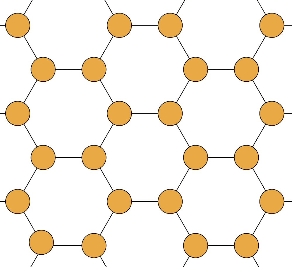
   Figure 1. Figure of the hexagonal tiling of the plane.

8. Geometric conditions for positive entropic curvature via the Motzkin-Strauss Theorem.

In positive curvature midpoints spread out. These considerations have been taken into account for the Ollivier’s coarse curvature (see [43, 44]). The following proposition shows that this property is also a necessary condition so that the lower bound $\inf_{z\in{\mathcal{X}}}r(z)$ of the entropic curvature of the graph space $({\mathcal{X}},d,L_{0},m_{0})$, due to Theorem 1, is positive.

Proposition 4.

Let $G=({\mathcal{X}},E)$ be a graph and let $z\in{\mathcal{X}}$ and let us suppose that $r(z)>0$ where $r(z):=-2\log K_{0}(z,S_{2}(z))$. Then the following properties hold :

1. for all $W\subset S_{2}(z)$ with $|W|\leq 2$ one has $|]z,W[|>|W|$.

2. for all $W\subset S_{2}(z)$ satisfying $]z,z^{\prime\prime}[=]z,w^{\prime\prime}[$ for all $z^{\prime\prime},w^{\prime\prime}\in W$, one has $|]z,W[|>|W|$.

We already have proved in comments (iii) of 1 that Proposition 4 holds for $|W|=1$. For $W:=\{z_{1}^{\prime\prime},z_{2}^{\prime\prime}\}$, if $\big{|}]z,W[\big{|}=2$ with $r(z)>0$ then necessarily $]z,W[=]z,z_{1}^{\prime\prime}[=]z,z_{2}^{\prime\prime}[=\{z_{1}^{\prime},z_{2}^{\prime}\}$ and therefore

$$K_{0}\big{(}z,S_{2}(z)\big{)}\geq\sup_{\alpha(z_{1}^{\prime})+\alpha(z_{2}^{\prime})=1}\big{\{}2\alpha(z_{1}^{\prime})\alpha(z_{2}^{\prime})+2\alpha(z_{1}^{\prime})\alpha(z_{2}^{\prime})\big{\}}=1.$$

This is a contradiction to the assumption that $r(z)>0$ and thus $\big{|}]z,W[\big{|}>2$. The proof of the last point of Proposition 4 is similar. Let $W\subset S_{2}(z)$ satisfying $]z,z^{\prime\prime}[=]z,w^{\prime\prime}[$ for all $z^{\prime\prime},w^{\prime\prime}\in W$, then $]z,z^{\prime\prime}[=]z,W[$ for all $z^{\prime\prime}\in W$ and therefore

$$K_{0}\big{(}z,S_{2}(z)\big{)}\geq\sup_{\alpha,\sum_{z^{\prime}\in S_{1}(z)}\alpha(z^{\prime})=1}\big{\{}\sum_{z^{\prime\prime}\in W}\big{|}]z,W[\big{|}\prod_{z^{\prime}\in]z,z^{\prime\prime}[}\alpha(z^{\prime})^{\frac{2}{\big{|}]z,W[\big{|}}}\big{\}}\geq\frac{|W|}{\big{|}]z,W[\big{|}},$$

where for the last inequality we choose $\alpha(z^{\prime})=\frac{1}{\big{|}]z,W[\big{|}}$ for all $z^{\prime}\in]z,W[$. As a consequence $r(z)>0$ implies $K_{0}\big{(}z,S_{2}(z)\big{)}<0$ and therefore $|W|<\big{|}]z,W[\big{|}$.

Actually, a natural guess for positive entropic curvature is the following one.

Conjecture 1.

Let $G=({\mathcal{X}},E)$ be a graph endowed with the counting measure. If for all $z\in{\mathcal{X}}$ and for all $W\subset S_{2}(z)$, $\big{|}]z,W[\big{|}>\big{|}W\big{|},$ then the graph space $G$ has positive entropic curvature.

The following two remarks show that the relationships between the cardinality of the midpoints and the lower bound on the entropic curvature given by $\inf_{z\in{\mathcal{X}}}r(z)$ are subtle.

• Given $z\in{\mathcal{X}}$, $r(z)>0$ does not imply that for all $W\subset S_{2}(z),\big{|}]z,W[\big{|}>\big{|}W\big{|}$. Indeed, assume that the graph $G=(V,E)$ restricted to the ball $B_{2}(z)$ is given by $S_{1}(z):=\{z_{1}^{\prime},z_{2}^{\prime},z_{3}^{\prime}\}$ and $S_{2}(z):=\{z_{1}^{\prime\prime},z_{2}^{\prime\prime},z_{3}^{\prime\prime}\}$ with $]z,z^{\prime\prime}_{1}[:=\{z_{1}^{\prime},z_{2}^{\prime}\}$, $]z,z^{\prime\prime}_{2}[:=\{z_{2}^{\prime},z_{3}^{\prime}\}$ and $]z,z^{\prime\prime}_{3}[:=\{z_{1}^{\prime},z_{3}^{\prime}\}$. Then it holds $K_{0}(z,S_{2}(z))=\sup_{\alpha}\big{\{}2\alpha(z_{1}^{\prime})\alpha(z_{2}^{\prime})+2\alpha(z_{2}^{\prime})\alpha(z_{3}^{\prime})+2\alpha(z_{1}^{\prime})\alpha(z_{3}^{\prime})\big{\}}=\frac{2}{3}<1$, and however for $W:=S_{2}(z)$ one has $\big{|}W\big{|}=\big{|}]z,W[\big{|}$.

• The following example shows that it is possible that the assumption of the conjecture 1 holds for a fixed vertex $z_{0}$ and that $r(z_{0})<0$. In fact, one will construct a family of balls $B_{2}(z_{0})$ indexed by $n\in\mathbb{N}^{*}$ for which for all $W\subset S_{2}(z_{0})$, $\big{|}]z_{0},W[\big{|}>\big{|}W\big{|}$ and show that for sufficiently large $n$, $r(z_{0})<0$. Let $S_{1}(z_{0}):=\{z_{1}^{\prime},z_{2}^{\prime},\ldots,z_{n+2}^{\prime}\}$ and $S_{2}(z_{0}):=\{z_{1}^{\prime\prime},z_{2}^{\prime\prime},\ldots,z_{n}^{\prime\prime}\}$ with for all $i\in[n]$, $]z_{0},z_{i}^{\prime\prime}[=\{z_{1}^{\prime},z_{2}^{\prime},z_{i+2}^{\prime}\}$.

  

  One easily check that for all $W\subset S_{2}(z_{0})$, $|]z_{0},W[|=|W|+1>|W|$. Moreover, it holds

  $$K_{0}\big{(}z_{0},S_{2}(z_{0})\big{)}=\sup_{\alpha,\sum_{i=1}^{n+2}\alpha(z_{i}^{\prime})=1}\sum_{i=1}^{n}3\big{(}\alpha(z_{1}^{\prime})\alpha(z_{2}^{\prime})\alpha(z_{i+2}^{\prime})\big{)}^{\frac{2}{3}}\geq 3n\big{(}\frac{1}{16}\cdot\frac{1}{2n}\big{)}^{\frac{2}{3}}=\frac{3}{32^{\frac{2}{3}}}n^{\frac{1}{3}}$$

  where for the last inequality we choose $\alpha(z_{1}^{\prime})=\alpha(z_{2}^{\prime})=\frac{1}{4}$ and $\alpha(z_{i}^{\prime})=\frac{1}{2n}$ for $i\in\{3,4,\ldots,n+2\}$. It follows that for $n\geq 38$, $K_{0}\big{(}z_{0},S_{2}(z_{0})\big{)}>1$ and therefore $r(z_{0})<0$.

Remark 3.

Note that the above construction is not a counterexample of conjecture 1 since we only assume that the hypotheses of the conjecture holds for a single $z_{0}$, and also since our criteria only gives a lower bound on the entropic curvature.

Let us now propose sufficient geometric conditions for positive entropic curvature related to the criteria $\inf_{z\in{\mathcal{X}}}r(z)<0$. One of the key ingredient of the results given below is the so-called Motzkin Strauss Theorem. In a seminal 1965 paper [40], Motzkin and Straus found an elegant relationship between the maximum clique of a graph and the global maxima of a quadratic optimization problem defined on the standard simplex. This connection produced another new proof of Turán’s theorem [40]. The Motzkin Strauss Theorem allows us to interpret the optimization problem which defines $K_{0}\big{(}z,S_{2}(z)\big{)}$ for some class of graphs as a problem of finding the maximum clique in a related graph. In order to be precise, one needs to introduce certain preliminary definitions.

Definition 6 (Clique, maximum clique and clique number).

Given a simple undirected graph $G^{*}=(V^{*},E^{*})$, a clique is a subset of vertices such that every two distinct vertices of this subset are adjacent. In other words, a clique is an induced subgraph of the graph $G^{*}$ that is complete. A maximum clique of $G^{*}$ is a clique with maximum cardinality. This maximum cardinality, denoted by $\omega(G^{*})$, is called the clique number of $G^{*}$.

Theorem 12.

[40] Let $G^{*}=(V^{*},E^{*})$ be a simple undirected graph with clique number $\omega(G^{*})$. Then the following relation holds,

$$2\max_{\alpha}\big{\{}\sum_{\{i,j\}\in E^{*}}\alpha_{i}\alpha_{j}\big{\}}=1-\frac{1}{\omega(G^{*})}\hskip 5.69046pt,$$

where the supremum runs overs all vectors $\alpha=(\alpha_{i})_{i\in V^{*}}$ with non negative coordinates and such that $\sum_{i\in V^{*}}\alpha_{i}=1$. Moreover the maximum is achieved by a characteristic vector $\alpha$ of a maximum clique $S$ of the graph $G^{*}$, that is : $\alpha_{i}=\frac{1}{\mid S\mid}$ for $i\in S$ and $\alpha_{i}=0$ otherwise.

Let $\mathcal{C}$ be the class of graphs $G=({\mathcal{X}},E)$ satisfying that any pair of vertices in ${\mathcal{X}}$ at distance two share two midpoints and two midpoints can not be shared by more than two vertices. Let $G$ be a graph of $\mathcal{C}$, and $z$ be a fixed vertex $z\in{\mathcal{X}}$. Let $G_{z}^{*}=(V_{z}^{*},E_{z}^{*})$ be the graph with set of vertices $V_{z}^{*}=S_{1}(z)$ and such that $\{z^{\prime},w^{\prime}\}$ is an edge of $E_{z}^{*}$ if $\{z^{\prime},w^{\prime}\}=]z,z^{\prime\prime}[$ for some $z^{\prime\prime}\in S_{2}(z)$. According to this construction, one exactly has

$$K_{0}\big{(}z,S_{2}(z)\big{)}=\sup_{\alpha}\Big{\{}2\sum_{\{z^{\prime},w^{\prime}\}\in E_{z}^{*}}\alpha(z^{\prime})\alpha(w^{\prime})\Big{\}}.$$

As a consequence, the next result is an easy application of Motzkin Strauss Theorem 12 together with Theorem 1.

Proposition 5.

Let $G=({\mathcal{X}},E)$ be a graph belonging to $\mathcal{C}$ and let $z$ be an arbitrary vertex of ${\mathcal{X}}$. Then, one has $K_{0}\big{(}z,S_{2}(z)\big{)}=1-\frac{1}{\omega(G^{*}_{z})}<1$, where $\omega(G^{*}_{z})$ is the clique number of the graph $G_{z}^{*}$ as defined above. As a consequence the entropic curvature of the graph space $G$ endowed with the counting measure is positive bounded from below by

$$\inf_{z\in{\mathcal{X}}}r(z)=\inf_{z\in{\mathcal{X}}}-2\log\Big{(}1-\frac{1}{\omega(G^{*}_{z})}\Big{)}\geq\frac{2}{\sup_{z\in{\mathcal{X}}}\omega(G^{*}_{z})}.$$

Comments:

• The following figure illustrates the construction of $G_{z}^{*}$ for a generic $G\in\mathcal{C}$:

  

  For this drawing example, one has $K_{0}(z,S_{2}(z))=1-\frac{1}{\omega(G_{z}^{*})}=\frac{2}{3}$.

• As an example, the hypercube ${\mathcal{X}}=\{0,1\}^{n}$ belongs to the class of graphs $\mathcal{C}$ and and for any $z\in{\mathcal{X}}$, $G_{z}^{*}$ is the complete graph on $n$ vertices $K_{n}$ with clique number $n$. One recovers the lower bound $-2\log(1-1/n)$ on the entropic curvature given in section 6.1.

• From a complexity point of view, the problem of computing the clique number is one of Karp’s 21 NP-hard problems [26]. Thus, it is immediate that the problem of calculating the entropic curvature of a graph is an NP-hard problem.

In the next proposition we consider another class of graphs satisfying the assumptions of Conjecture 1, together with a covering condition. For this class of graphs we also derive positive entropic curvature by applying the Motzkin Strauss Theorem.

Proposition 6.

Let $G=({\mathcal{X}},E)$ be a graph. Assume that for any arbitrary vertex $z$ of ${\mathcal{X}}$ and for any three distinct vertices $z_{1}^{\prime\prime},z_{2}^{\prime\prime},z_{3}^{\prime\prime}$ of $S_{2}(z)$,

(57) $$]z,z_{1}^{\prime\prime}[\cap]z,z_{2}^{\prime\prime}[\cap]z,z_{3}^{\prime\prime}[=\emptyset.$$

Assume also that for all subsets $W\subset S_{2}(z)$ of cardinality one or two, one has

(58) $$\big{|}]z,W[\big{|}>|W|.$$

Then one gets $K\big{(}z,S_{2}(z)\big{)}\leq 7/8$ and Theorem 1 ensures that the entropic curvature of the graph space $G$ endowed with the counting measure is bounded from below by $1/4$.

Remark 4.

Note that the hypothesis (57) implies that there is no overlapping of more than three midpoint sets. It is still an open problem to generalize this type of results to larger overlapping.

9. Few comparisons with other notions of curvature.

Recall that according to the comments of Theorem 1, the entropic curvature of the graph space $G=({\mathcal{X}},d,m_{0},L_{0})$ is lower bounded by $\inf_{z\in{\mathcal{X}}}r(z)$ where $r(z):=-2\log K_{0}(z,S_{2}(z)$ is interpreted as a local lower bound on the entropic curvature. In this section we give some comparative remarks between this lower bound and the notions of curvature by Lin-Lu-Yau and Bakry-Émery.

Some relations between entropic curvature and the Lin-Lu-Yau curvature.

The Lin-Lu-Yau curvature is a modified notion of the coarse Ollivier’s Ricci curvature introduced by Lin, Lu and Yau in [32]. In [41], Florentin Münch and Radosław K.Wojciechowski, generalized the notion of Lin-Lu-Yau curvature for any graph Laplacian.

Definition 7 (Lin-Lu-Yau Ricci curvature).

Given $G=(\mathcal{X},E)$ a graph endowed with its graph distance $d$ and with a Markov chain defined by $m:=\{m_{z}(\cdot)\}_{z\in\mathcal{X}}$. For $0\leq\alpha<1$, the $\alpha$-lazy random walk $m_{x}^{\alpha}$ associated to the graph Laplacian $L_{0}$ is defined as

$$m_{x}^{\alpha}(y)=\begin{cases}\frac{\alpha}{\Delta(G)}\hskip 5.69046pt\text{if}\hskip 5.69046ptx\sim y,\\ 1-\alpha\frac{\text{deg }(x)}{\Delta(G)}\hskip 5.69046pt\text{if}\hskip 5.69046pty=x,\\ 0\hskip 5.69046pt\text{otherwise}.\end{cases}$$

For every $x,y\in\mathcal{X}$, one defines

$$\kappa_{\alpha}(x,y):=1-\frac{W_{1}(m_{x}^{\alpha},m_{y}^{\alpha})}{d(x,y)}.$$

As shown in [41], the limit as $\alpha\rightarrow 0$ exists for any graph Laplacian and therefore one can define the Ricci Lin-Lu-Yau curvature along the edge $\{x,y\}$ denoted as $\kappa_{LLY}(x,y)$ by

$$\kappa_{LLY}(x,y):=\lim_{\alpha\rightarrow 0}\frac{\kappa_{\alpha}(x,y)}{\alpha}.$$

The next proposition establishes a link between the Lin-Lu-Yau curvature and the graph-theoretical notion of girth.

Definition 8.

The girth of a graph $G=(\mathcal{X},E)$, denoted $g(G)$ is the length of the shortest cycle contained in $G$. Acyclic graphs are considered to have infinite girth.

Adapting the proof [10, Theorem 2.b(ii)], provides the following proposition with the measures $m_{x}^{\alpha}$ associated to the generator $L_{0}$. Its proof is postponed in Appendix B.

Proposition 7.

Let $G=(\mathcal{X},E)$ be a graph. If for all $x,y\in\mathcal{X}$ with $d(x,y)=1$

$$\kappa_{LLY}(x,y)<\frac{6-\text{deg}(x)-\text{deg}(y)}{\Delta(G)}$$

then $g(G)\geq 5$.

Remark 5.

Let $G=(\mathcal{X},E)$ be a graph . If $g(G)\geq 5$, then there cannot be two midpoints between two vertices at distance two and thus as already noted in the introduction for all $z\in\mathcal{X}$, $r(z)\leq 0$.

Thanks to the above remark, by contraposition, we immediately obtain the following corollary.

Corollary 2.

Let $G=(\mathcal{X},E)$ be a graph. If for all $z\in{\mathcal{X}}$, $r(z)>0$, then for all $x,y\in\mathcal{X}$ with $d(x,y)=1$,

$$\kappa_{LLY}(x,y)\geq\frac{6-\text{deg(x)}-\text{deg(y)}}{\Delta(G)}\hskip 2.84544pt.$$

Observe that $\kappa_{LLY}(x,y)>0$ does not imply $r(x)>0$ nor that $r(y)>0$. Indeed, let us consider the so-called windmill graph $W_{d}(4,2)$, consisting of 2 copies of the complete graph $K_{4}$ at a shared universal vertex:

For the edge $\{x,y\}$ of the graph $W_{d}(4,2)$ on the figure, $\kappa_{LLY}(x,y)=2/3$ (one may easily check that $W_{1}(m_{x}^{\alpha},m_{y}^{\alpha})=1-\frac{\alpha}{2}-\frac{\alpha}{6}$). However, one has $K_{0}\big{(}x,S_{2}(x)\big{)}=K_{0}\big{(}y,S_{2}(y)\big{)}=3$ and thus $r(x)=r(y)<0$.

Some comparative aspects between entropic curvature and the Bakry-Émery curvature condition.

There are relationships between the entropic curvature and the Bakry-Émery curvature. The notion of Bakry-Émery curvature was first introduced by Bakry and Émery in [4]. The Bakry-Émery curvature is motivated by the Bochner’s identity in Riemannian Geometry and has been extensively studied in discrete spaces recently [14, 15]. Let us make some qualitative remarks on the similarities with respect to the local structure and the negativity of curvature for both notions.

In the case where $L=L_{0}$, the works [14, 15] show that the Bakry-Émery conditions are also related to the local structure of balls of radius 2. More precisely, the curvature matrix for a vertex $z\in\mathcal{X}$ is completely determined by the incomplete ball of radius 2 around $z$, that is, the graph induced by $B_{2}(z)$ removing all edges connecting vertices within $S_{2}(z)$ (see [14, Remark 2.2]). Similarly, the lower bound $r(z)$ interpreted as the local entropic curvature at vertex $z$ only depends on this incomplete ball of radius 2 removing also all edges connecting vertices within $S_{1}(z)$.

Moreover, according to [15, Theorem 6.4], if the punctured 2-ball around $z$, defined as the incomplete ball of radius 2 from which we remove all edges connected to $z$, has more than one connected component then the Bakry-Émery curvature criterion at the vertex $z$ is negative with five exceptions (see [15, Theorem 6.4]). In this configuration, choosing $z^{\prime}\in S_{1}(z)$ in one component of the punctured 2-ball, the quantity $r(z^{\prime})$ is less or equal to zero. Indeed, since the punctured 2-ball around $z$ has more than one connected component there exists $w^{\prime}\in S_{2}(z^{\prime})\cap S_{1}(z)$ such that $z\in S_{1}(z^{\prime})$ is the unique midpoint between $z^{\prime}$ and $w^{\prime}$. As an immediate consequence (see [15, Corollary 6.8]), if a graph has girth greater than or equal to five, then the Bakry-Émery curvature criterion at each vertex is less than zero. Recall that in our setting, girth greater or equal to five implies $r(z)\leq 0$ for all vertices $z$ (see Remark 5).

10. Appendix A

Lemma 4.

Let ${\mathcal{X}}$ be a structured graph associated to a set of moves ${\mathcal{S}}$. Then the following properties hold :

1. Given $d\in{\mathbb{N}}$, $\tau\in{\mathcal{S}}$ and $\alpha_{0},\ldots,\alpha_{d}\in{\mathcal{X}}$, if $\big{(}\alpha_{0},\ldots,\alpha_{d},\tau(\alpha_{d})\big{)}\in G\big{(}\alpha_{0},\tau(\alpha_{d})\big{)}$ then for any $k\in\{0,\ldots,d\}$ one has $\big{(}\alpha_{0},\ldots,\alpha_{k},\tau(\alpha_{k}),\ldots,\tau(\alpha_{d})\big{)}\in G\big{(}\alpha_{0},\tau(\alpha_{d})\big{)}$. If moreover the generator $L$ on ${\mathcal{X}}$ satisfies condition (28), then one has

   $$L\big{(}\alpha_{0},\ldots,\alpha_{d},\tau(\alpha_{d})\big{)}=L\big{(}\alpha_{0},\ldots,\alpha_{k},\tau(\alpha_{k}),\ldots,\tau(\alpha_{d})\big{)}.$$

2. For any $x,y,z\in{\mathcal{X}}$ and $\tau\in{\mathcal{S}}$ with $\tau(z)\sim z$, if $(z,\tau(z))\in[x,y]$ then $\tau(x)\in]x,y]$ and $\tau(z)\in[\tau(x),y]$.

3. Let $z\in{\mathcal{X}}$ and $\tau,\sigma_{1},\sigma_{2}\in{\mathcal{S}}$ such that $d\big{(}z,\tau\sigma_{1}(z)\big{)}=2$ and $\tau\sigma_{1}(z)=\tau\sigma_{2}(z)$. Then one has $\sigma_{1}=\sigma_{2}$.

4. Let $d\in{\mathbb{N}}^{*}$, $\tau\in{\mathcal{S}}$ and $\alpha_{0},\beta_{2},\ldots\beta_{d+1}\in{\mathcal{X}}$. If $(\alpha_{0},\tau(\alpha_{0}),\beta_{2},\ldots,\beta_{d+1})\in G(\alpha_{0},\beta_{d+1})$ then for any $k\in\{0,\ldots,d\}$, there exists a single $(\alpha_{0},\alpha_{1},\ldots,\alpha_{k})\in{\mathcal{X}}^{k+1}$ such that

   $$(\alpha_{0},\alpha_{1},\ldots,\alpha_{k},\tau(\alpha_{k}),\beta_{k+2},\ldots,\beta_{d+1})\in G(\alpha_{0},\beta_{d+1}),$$

   and for any $\ell\in[k]$, $\beta_{\ell+1}=\tau(\alpha_{\ell})$.

5. Given $d\in{\mathbb{N}}^{*}$, $\tau\in{\mathcal{S}}$ and $\alpha_{0}\in{\mathcal{X}}$, let

   $${\mathcal{Y}}(\alpha_{0},\tau,d):=\big{\{}(\alpha_{1},\ldots,\alpha_{d+1})\in{\mathcal{X}}^{d+1}\,\big{|}\,(\alpha_{0},\ldots,\alpha_{d},\alpha_{d+1})\in G(\alpha_{0},\alpha_{d+1}),\alpha_{d+1}=\tau(\alpha_{d})\big{\}},$$

   and

   $${\mathcal{W}}(\alpha_{0},\tau,d):=\big{\{}(\beta_{2},\ldots,\beta_{d+1})\in{\mathcal{X}}^{d}\,\big{|}\,(\alpha_{0},\tau(\alpha_{0}),\beta_{2},\ldots,\beta_{d+1})\in G(\alpha_{0},\beta_{d+1})\big{\}}.$$

   The map $\Psi:(\alpha_{1},\ldots,\alpha_{d+1})\mapsto(\tau(\alpha_{1}),\ldots,\tau(\alpha_{d}))$ is one to one from the set ${\mathcal{Y}}(\alpha_{0},\tau,d)$ to the set ${\mathcal{W}}(\alpha_{0},\tau,d)$.

6. Assume that $L$ is a generator on ${\mathcal{X}}$ satisfying condition (28). Let $x,y\in{\mathcal{X}}$ and $\tau\in{\mathcal{S}}$ such that $\tau(x)\in]x,y]$ and let $k\in\{0,\ldots,d-1\}$ where $d=d(x,y)-1$. Then one has

   $$\sum_{z\in{\mathcal{X}},d(x,z)=k,(z,\tau(z))\in[x,y]}L^{k}(x,z)L(z,\tau(z))L^{d-k-1}(\tau(z),y)=L(x,\tau(x))L^{d-1}(\tau(x),y).$$

Proof.

The proof of (i) is by induction over $k\in\{0,\ldots,d\}$. The property holds for $k=d$ by assumption. Assume that for some fixed $k\in[d]$, $\big{(}\alpha_{0},\ldots,\alpha_{k},\tau(\alpha_{k}),\ldots,\tau(\alpha_{d})\big{)}$ is a discrete geodesic. Then since $d(\alpha_{k-1},\alpha_{k})=1$, there exists a single $\sigma_{k}\in{\mathcal{S}}$ such that $\sigma_{k}(\alpha_{k-1})=\alpha_{k}$. Since $d\big{(}\alpha_{k-1},\tau(\alpha_{k})\big{)}=d\big{(}\alpha_{k-1},\tau\sigma_{k}(\alpha_{k-1})\big{)}=2$, according to the definition of structured graphs, there exists $\psi(\sigma_{k})\in{\mathcal{S}}_{\tau(\alpha_{k-1})}$ such that

$$\tau\sigma_{k}(\alpha_{k-1})=\psi(\sigma_{k})\tau(\alpha_{k-1}).$$

Therefore one has $\tau(\alpha_{k-1})\in]\alpha_{k-1},\tau(\alpha_{k})[$ and $(\alpha_{0},\ldots,\alpha_{k-1},\tau(\alpha_{k-1}),\ldots,\tau(\alpha_{d}))$ is a discrete geodesic. If moreover condition (28) holds, then by induction hypothesis

$$L\big{(}\alpha_{0},\ldots,\alpha_{k-1},\tau(\alpha_{k-1}),\ldots,\tau(\alpha_{d})\big{)}$$

$$=L\big{(}\alpha_{0},\ldots,\alpha_{k-1}\big{)}L\big{(}\alpha_{k-1},\tau(\alpha_{k-1})\big{)}L\big{(}\tau(\alpha_{k-1}),\tau\sigma_{k}(\alpha_{k-1})\big{)}L\big{(}\tau(\alpha_{k}),\ldots,\tau(\alpha_{d})\big{)}$$

$$=L\big{(}\alpha_{0},\ldots,\alpha_{k-1}\big{)}L\big{(}\alpha_{k-1},\sigma_{k}(\alpha_{k-1})\big{)}L\big{(}\sigma_{k}(\alpha_{k-1}),\tau\sigma_{k}(\alpha_{k-1})\big{)}L\big{(}\tau(\alpha_{k}),\ldots,\tau(\alpha_{d})\big{)}$$

$$=L\big{(}\alpha_{0},\ldots,\alpha_{k},\tau(\alpha_{k}),\ldots,\tau(\alpha_{d})\big{)}$$

$$=L\big{(}\alpha_{0},\ldots,\alpha_{d},\tau(\alpha_{d})\big{)}.$$

Item (ii) is an easy consequence of (i). Indeed, if $(z,\tau(z))\in[x,y]$ then, setting $d=d(x,y)$ and $k=d(x,z)$, there exists $(\alpha_{0},\alpha_{1},\ldots,\alpha_{k},\tau(\alpha_{k}),\beta_{k+2},\ldots,\beta_{d})\in G(x,y)$ with $\alpha_{k}=z$. Item (i) implies that

$$(x,\tau(x),\tau(\alpha_{1}),\ldots,\tau(\alpha_{k}),\beta_{k+2},\ldots,\beta_{d})=(\alpha_{0},\tau(\alpha_{0}),\ldots,\tau(\alpha_{k}),\beta_{k+2},\ldots,\beta_{d})\in G(x,y),$$

and therefore $\tau(x)\in]x,y]$ and $\tau(z)\in[\tau(x),y]$.

For the proof of (iii), let $z\in{\mathcal{X}}$ and $\sigma_{1},\sigma_{2},\tau\in{\mathcal{S}}$ such that $d\big{(}z,\tau\sigma_{1}(z)\big{)}=2$. If $\tau\sigma_{1}(z)=\tau\sigma_{2}(z)$ then according to the definition of structured graphs $\psi(\sigma_{1})\tau(z)=\psi(\sigma_{2})\tau(z)$. It follows that $\psi(\sigma_{1})=\psi(\sigma_{2})$ and therefore $\sigma_{1}=\sigma_{2}$ since the map $\psi$ is one to one.

The proof of (iv) is by induction over $k\in\{0,\ldots,d\}$. The property holds for $k=0$ by assumption. Assume that for a fixed $k\in\{0,\ldots,d-1\}$, there exists a single $(\alpha_{0},\alpha_{1},\ldots,\alpha_{k})\in{\mathcal{X}}^{k+1}$ such that

$$(\alpha_{0},\alpha_{1},\ldots,\alpha_{k},\tau(\alpha_{k}),\beta_{k+2},\ldots,\beta_{d+1})\in G(\alpha_{0},\beta_{d+1}),$$

and for any $\ell\in[k]$, $\beta_{\ell+1}=\tau(\alpha_{\ell})$. According to the definition of structured graphs, since $d(\tau(\alpha_{k}),\beta_{k+2})=1$, there exists a single $\sigma_{k+1}^{\prime}\in{\mathcal{S}}_{\tau(\alpha_{k})}$ such that $\beta_{k+2}=\sigma_{k+1}^{\prime}\tau(\alpha_{k})$, and since $d\big{(}\alpha_{k},\sigma_{k+1}^{\prime}\tau(\alpha_{k})\big{)}=2$, one has

$$\beta_{k+2}=\sigma_{k+1}^{\prime}\tau(\alpha_{k})=\tau\psi^{-1}(\sigma_{k+1}^{\prime})(\alpha_{k}).$$

Setting $\alpha_{k+1}=\psi^{-1}(\sigma_{k+1}^{\prime})(\alpha_{k})$, one has $\beta_{k+2}=\tau(\alpha_{k+1})$ and since $\alpha_{k+1}\in]\alpha_{k},\beta_{k+2}[$ it follows that

$$(\alpha_{0},\alpha_{1},\ldots,\alpha_{k+1},\tau(\alpha_{k+1}),\beta_{k+3},\ldots,\beta_{d+1})\in G(\alpha_{0},\beta_{d+1}).$$

Moreover if $\alpha^{\prime}_{k+1}$ is such that $\beta_{k+2}=\tau(\alpha_{k+1}^{\prime})$ and

$$(\alpha_{0},\alpha_{1},\ldots,\alpha_{k},\alpha_{k+1}^{\prime},\tau(\alpha_{k+1}^{\prime}),\beta_{k+3},\ldots,\beta_{d+1})\in G(\alpha_{0},\beta_{d+1}),$$

then there exists $\sigma_{k+1}$ such that $\alpha_{k+1}^{\prime}=\sigma_{k+1}(\alpha_{k})$. Applying (iii), it follows that $\psi(\sigma_{k+1})=\sigma_{k+1}^{\prime}$ and therefore

$$\alpha_{k+1}^{\prime}=\sigma_{k+1}(\alpha_{k})=\psi^{-1}(\sigma_{k+1}^{\prime})(\alpha_{k})=\alpha_{k+1}.$$

This ends the proof of (iv).

We now turn to the proof of (v). Let $d\in{\mathbb{N}}^{*}$, $\tau\in{\mathcal{S}}$ and $\alpha_{0}\in{\mathcal{X}}$. If $(\alpha_{1},\ldots,\alpha_{d+1})\in{\mathcal{Y}}(\alpha_{0},\tau,d)$ then according to (i) with $k=0$, one has

$$(\alpha_{0},\tau(\alpha_{0}),\ldots,\tau(\alpha_{d}))\in G(\alpha_{0},\tau(\alpha_{d})),$$

and therefore $\Psi(\alpha_{1},\ldots,\alpha_{d+1})\in{\mathcal{W}}(\alpha_{0},\tau,d)$. Conversely if $(\beta_{2},\ldots,\beta_{d+1})\in{\mathcal{W}}(\alpha_{0},\tau,d)$, then

$$(\alpha_{0},\tau(\alpha_{0}),\beta_{2},\ldots,\beta_{d+1})\in G(\alpha_{0},\beta_{d+1}),$$

and according to (iv) for $k=d$, there exists a single $(\alpha_{0},\ldots,\alpha_{d})$ such that

$$(\alpha_{0},\alpha_{1},\ldots,\alpha_{d},\tau(\alpha_{d}))\in G(\alpha_{0},\beta_{d+1}),$$

and for all $\ell\in[d]$, $\beta_{\ell+1}=\tau(\alpha_{\ell})$. Therefore, there exists a single $(\alpha_{1},\ldots,\alpha_{d})\in{\mathcal{Y}}(\alpha_{0},\tau,d)$ such that $\psi(\alpha_{1},\ldots,\alpha_{d})=(\beta_{2},\ldots,\beta_{d+1})$.

For the proof of (vi), let $L$ be a generator on ${\mathcal{X}}$ satisfying condition (28), let $x,y\in{\mathcal{X}}$ and $\tau\in{\mathcal{S}}$ such that $\tau(x)\in]x,y]$ and let $k\in\{0,\ldots,d-1\}$ where $d=d(x,y)-1$. By definition, one has

$$\sum_{z\in{\mathcal{X}},d(x,z)=k,(z,\tau(z))\in[x,y]}L^{k}(x,z)L(z,\tau(z))L^{d-k-1}(\tau(z),y)\\ =\sum_{(\alpha_{1},\ldots,\alpha_{k+1})\in{\mathcal{Y}}(x,\tau,k)}\sum_{\gamma\in G(\tau(\alpha_{k}),y)}L(x,\alpha_{1},\ldots,\alpha_{k+1})\,L(\gamma).$$

Applying (i) and then (v) it follows that

$$\sum_{z\in{\mathcal{X}},d(x,z)=k,(z,\tau(z))\in[x,y]} L^{k}(x,z)L(z,\tau(z))L^{d-k-1}(\tau(z),y)$$

$$=\sum_{(\alpha_{1},\ldots,\alpha_{k})\in{\mathcal{Y}}(x,\tau,k)}\sum_{\gamma\in G(\tau(\alpha_{k}),y)}L(x,\tau(x),\tau(\alpha_{1}),\ldots,\tau(\alpha_{k}))\,L(\gamma)$$

$$=\sum_{(\beta_{2},\ldots,\beta_{k+1})\in{\mathcal{W}}(x,\tau,k)}\sum_{\gamma\in G(\beta_{k+1},y)}L(x,\tau(x),\beta_{2},\ldots,\beta_{k+1})\,L(\gamma)$$

$$=L(x,\tau(x))\sum_{\gamma^{\prime}\in G(\tau(x),y)}L(\gamma^{\prime})=L(x,\tau(x))L^{d-1}(\tau(x),y).$$

The proof of Lemma 4 is completed. ∎

Lemma 5.

Let $({\mathcal{X}},d,m,L)$ be a graph space. Let $v:{\mathcal{X}}\to{\mathbb{R}}$ be a bounded function and given $x,y\in{\mathcal{X}}$ let

$$R(t)=\int v\,d\nu_{t}^{x,y},\qquad t\in(0,1),$$

where $(\nu_{t}^{x,y})_{t\in[0,1]}$ is the Schrödinger path between Dirac measures at $x$ and $y$ defined by (5). One has for any $t\in[0,1]$,

$$R^{\prime\prime}(t):=d(x,y)\big{(}d(x,y)-1\big{)}\,D_{t}v(x,y),$$

with

$$D_{t}v(x,y):=\sum_{(z,z^{\prime\prime})\in[x,y],d(z,z^{\prime\prime})=2}\left[\sum_{z^{\prime}\in]z,z^{\prime\prime}[}\left(v(z^{\prime\prime})+v(z)-2v(z^{\prime})\right)L(z,z^{\prime})L(z^{\prime},z^{\prime\prime})\right]\\ r(x,z,z^{\prime\prime},y)\,\rho_{t}^{d(x,y)-2}(d(x,z))$$

Proof of Lemma 5.

Let $d:=d(x,y)$. For $t\in[0,1]$, one has

$$R(t)=\sum_{k=0}^{d}\rho_{t}^{d}(k)R_{k},\quad\mbox{ with}\quad R_{k}:=\sum_{z\in[x,y],d(x,z)=k}v(z)\,\frac{L^{d(x,z)}(x,z)L^{d(z,y)}(z,y)}{L^{d}(x,y)}$$

Simple computations give for any $t\in[0,1]$,

$$R^{\prime}(t)=d\,\sum_{k=0}^{d-1}\rho_{t}^{d-1}(k)\big{(}R_{k+1}-R_{k}\big{)},$$

and therefore

$$R^{\prime\prime}(t)=d(d-1)\,\sum_{k=0}^{d-2}\rho_{t}^{d-2}(k)\big{(}R_{k+2}+R_{k}-2R_{k+1}\big{)}.$$

Then the result follows observing that for any $k\in\{0,\ldots,d-2\}$,

$$R_{k+2}+R_{k}-2R_{k+1}$$

$$=\sum_{(z,z^{\prime},z^{\prime\prime})\in[x,y],d(x,z)=k}\left(v(z^{\prime\prime})+v(z)-2v(z^{\prime})\right)\frac{L^{d(x,z)}(x,z)L(z,z^{\prime})L(z^{\prime},z^{\prime\prime})L^{d(z^{\prime\prime},y)}(z^{\prime\prime},y)}{L^{d}(x,y)}$$

$$=\sum_{(z,z^{\prime\prime})\in[x,y]d(x,z)=k,d(z,z^{\prime\prime})=2}\left[\sum_{z^{\prime}\in]z,z^{\prime\prime}[}\left(v(z^{\prime\prime})+v(z)-2v(z^{\prime})\right)L(z,z^{\prime})L(z^{\prime},z^{\prime\prime})\right]r(x,z,z^{\prime\prime},y).$$

∎

Proposition 8.

Let $G=({\mathcal{X}},E)$ be a structured graph with finite set of moves ${\mathcal{S}}$. Let us suppose that moves in ${\mathcal{S}}$ commute, that is, $\sigma\tau=\tau\sigma$ for all $\sigma,\tau\in{\mathcal{S}}$. Then the Bakry-Émery curvature criterion $CD(0,\infty)$ is satisfied for every $z\in{\mathcal{X}}$.

Note that the commutativity condition is not necessary for structured graphs to satisfy the $CD(0,\infty)$ criterion. Indeed, the Bernoulli-Laplace model corresponds to a non-commutative structured graph with positive Bakry-Émery curvature as shown in [27, Theorem 2.7].

Proof of Proposition 8.

Let us recall the definition of the Bakry-Émery curvature condition in a graph space equipped with the generator $L_{0}$. Let $\Gamma$ and $\Gamma_{2}$ be symmetric operators defined respectively as

$$2\Gamma(f,g) :=L_{0}(fg)-fL_{0}g-gL_{0}f,$$

$$2\Gamma_{2}(f,g) :=L_{0}(\Gamma(f,g))-\Gamma(f,L_{0}g)-\Gamma(g,L_{0}f)$$

for all real function $f$ and $g$ on ${\mathcal{X}}$, where $L_{0}(f)$ is the discrete Laplace operator. As a convention $\Gamma(f):=\Gamma(f,f)$ and $\Gamma_{2}(f):=\Gamma_{2}(f,f)$.

Definition 9.

[33, 48, Bakry-Émery curvature condition] A vertex $z\in\mathcal{X}$ satisfies the Bakry-Émery curvature-dimension inequality $CD(\kappa_{BE},N)$ with $\kappa_{BE}\in\mathbb{R}$ and $N\in(0,\infty]$, if for any $f:\mathcal{X}\rightarrow\mathbb{R}$

$$\Gamma_{2}(f)(z)\geq\frac{1}{N}(L_{0}f(z))^{2}+\kappa_{BE}\Gamma(f)(z),$$

where $N$ is a dimension parameter and $\kappa_{BE}$ is regarded as a lower Ricci bound at $z\in{\mathcal{X}}$.

We want to prove that for any vertex $z$ of a structured graph whose moves in ${\mathcal{S}}$ commute, one has $\Gamma_{2}(f)(z)\geq 0$.

Following the same computations as in [12, 33, 13], one has

$$L_{0}\Gamma(f)(z) =\sum_{\sigma\in{\mathcal{S}},\sigma(z)\sim z}\big{(}\Gamma(f)(\sigma(z))-\Gamma(f)(z)\big{)}$$

$$=\frac{1}{2}\sum_{\sigma,\sigma(z)\sim z}\;\sum_{\tau,\tau(z)\sim z}\big{(}f(\tau\sigma(z))-f(\sigma(z))-f(\tau(z))+f(z)\big{)}^{2}$$

$$+\sum_{\sigma,\sigma(z)\sim z}\;\sum_{\tau,\tau(z)\sim z}(f(\tau(z))-f(z))(f(\tau\sigma(z))-f(\sigma(z))-f(\tau(z))+f(z))$$

where we have used the identity $A^{2}-B^{2}=(A-B)^{2}+2B(A-B)$, and

$$-2\Gamma(f,\L_{0}f)(z) =-\sum_{\tau,\tau(z)\sim z}(f(\tau(z))-f(z))(L_{0}f(\tau(z))-L_{0}f(z))$$

$$=-\sum_{\sigma,\sigma(z)\sim z}\;\sum_{\tau,\tau(z)\sim z}(f(\tau(z))-f(z))(f(\sigma\tau(z))-f(\sigma(z))-f(\tau(z))+f(z)).$$

From the commutativity assumption $\sigma\tau=\tau\sigma$, and summing up one gets

$$2\Gamma_{2}(f)(z)=\frac{1}{2}\sum_{\sigma,\sigma(z)\sim z}\;\sum_{\tau,\tau(z)\sim z}(f(\tau\sigma(z))-f(\sigma(z))-f(\tau(z))+f(z))^{2}\geq 0.$$

∎

11. Appendix B

11.1. Proofs of Theorem 1, Theorem 2 and Theorem 7

Proof of Theorem 1.

Theorem 1 is a consequence of Lemma 3.1 and Theorem 3.5 of [47]. The results of this paper [47] are given for graph spaces and the two following additional assumptions : the measure $m$ is uniformly upper bounded and lower bounded away from 0,

$$\sup_{x\in{\mathcal{X}}}m(x)<\infty,\qquad\inf_{x\in{\mathcal{X}}}m(x)>0,$$

and the generator $L$ is uniformly upper bounded, and uniformly lower bounded away from zero on the set of neighbours,

$$\sup_{x\in{\mathcal{X}}}|L(x,x)|<\infty,\qquad\inf_{x,y\in{\mathcal{X}},d(x,y)=1}L(x,y)>0.$$

These conditions are not in the setting of Theorem 1. To overcome this difficulty, one will consider a well chosen space $({\mathcal{C}},d,L_{\mathcal{C}},m_{\mathcal{C}})$ defined as the restriction of the space $({\mathcal{X}},d,m,L)$ to a well chosen finite convex subset ${\mathcal{C}}$ as defined in section 4.2.

Let $\nu_{0}$ and $\nu_{1}$ be two probability measures on ${\mathcal{X}}$ with bounded support. Since each vertex has bounded degree, there exists a finite convex subset ${\mathcal{C}}$ of ${\mathcal{X}}$ that contains all the balls of radius 2 with center in the finite subset $[\mathrm{supp}(\nu_{0}),\mathrm{supp}(\nu_{1})]$. Choose for example the convex subset ${\mathcal{C}}$ with minimal elements. Let $(\widehat{\nu}_{t})_{t\in[0,1]}$ denotes the Schrödinger bridge at zero temperature selected from the slowing down procedure on the space $({\mathcal{C}},d,L_{\mathcal{C}},m_{\mathcal{C}})$. As explained in [47] there exists a $W_{1}$-optimal coupling $\widehat{\pi}$ with marginals $\nu_{0}$ and $\nu_{1}$ such that the expression of $(\widehat{\nu}_{t})_{t\in[0,1]}$ is given by (4) on the space $({\mathcal{C}},d,L_{\mathcal{C}},m_{\mathcal{C}})$. Due to the assumption on the subset ${\mathcal{C}}$, for any $(x,y)\in\mathrm{supp}\widehat{\pi}$, the set $[x,y]$ is the same on the space $({\mathcal{X}},d,m,L)$ and on the space $({\mathcal{C}},d,L_{\mathcal{C}},m_{\mathcal{C}})$. Moreover, since $L_{\mathcal{C}}(x,y)=L(x,y)$ for $x\neq y$, the expression of $r(x,z,z,y)$ for $z\in[x,y]$ and $(x,y)\in\mathrm{supp}(\widehat{\pi})$ is also the same on $({\mathcal{X}},d,m,L)$ and on $({\mathcal{C}},d,L_{\mathcal{C}},m_{\mathcal{C}})$. Therefore the expression of the Schrödinger bridges between Dirac measure $\delta_{x}$ and $\delta_{y}$ is for us given by (5) does not depend on the chosen convex subset ${\mathcal{C}}$. Up to now we are working on $({\mathcal{C}},d,L_{\mathcal{C}},m_{\mathcal{C}})$ but for most of all expressions we write, there is no dependence in ${\mathcal{C}}$ or the subset ${\mathcal{C}}$ may be replaced by ${\mathcal{X}}$.

As already mentioned, he subset $\mathrm{supp}\,\widehat{\pi}$ is $d$-cyclically monotone. According to the definitions introduced in section 2, for any $t\in(0,1)$ the support of $\widehat{\nu}_{t}$ is given by

$$\mathrm{supp}(\widehat{\nu}_{t})=\widehat{Z}:=Z(\mathrm{supp}\,\widehat{\pi})=\bigcup_{(x,y)\in\mathrm{supp}\,\widehat{\pi}}[x,y].$$

and one denotes $C_{{}_{\rightarrow}}:=C_{{}_{\rightarrow}}(\mathrm{supp}\,\widehat{\pi})$, $C_{{}_{\leftarrow}}:=C_{{}_{\leftarrow}}(\mathrm{supp}\,\widehat{\pi})$, and for any $z\in\widehat{Z}$

$$V_{{}_{\rightarrow}}(z):=V_{{}_{\rightarrow}}^{\mathrm{supp}\,\widehat{\pi}}(z),\quad V_{{}_{\leftarrow}}(z):=V_{{}_{\leftarrow}}^{\mathrm{supp}\,\widehat{\pi}}(z),\quad{\mathbb{V}}_{{}_{\rightarrow}}(z):={\mathbb{V}}_{{}_{\rightarrow}}^{\mathrm{supp}\,\widehat{\pi}}(z),\quad{\mathbb{V}}_{{}_{\leftarrow}}(z):={\mathbb{V}}_{{}_{\leftarrow}}^{\mathrm{supp}\,\widehat{\pi}}(z).$$

For any $z\in\widehat{Z}$ let also

$$\widehat{Y}_{z}:=\Big{\{}y\in\mathrm{supp}(\nu_{1})\,\Big{|}\,\exists x\in{\mathcal{X}},(x,y)\in\widehat{\pi},z\in[x,y]\Big{\}},$$

and identically let

$$\widehat{X}_{z}:=\Big{\{}x\in\mathrm{supp}(\nu_{0})\,\Big{|}\,\exists y\in{\mathcal{X}},(x,y)\in\widehat{\pi},z\in[x,y]\Big{\}}.$$

For $y\in\mathrm{supp}(\nu_{1})$, $z\in{\mathcal{X}}$ and $t\in[0,1]$, the quantity

$$a_{t}(z,y):=\int\nu_{t}^{w,y}(z)\,d\widehat{\pi}_{{}_{\leftarrow}}(w|y),$$

is positive if and only if $z\in\widehat{Z}$ and $y\in\widehat{Y}_{z}$. Identically, for $x\in\mathrm{supp}(\nu_{0})$, $z\in{\mathcal{X}}$ and $t\in[0,1]$, the quantity

$$b_{t}(z,x):=\int\nu_{t}^{x,w}(z)\,d\widehat{\pi}_{{}_{\rightarrow}}(w|x),$$

is positive if and only if $z\in\widehat{Z}$ and $x\in\widehat{X}_{z}$. Actually $a_{t}$ and $b_{t}$ represent conditional laws, $\sum_{z\in{\mathcal{X}}}a_{t}(z,y)=\sum_{z\in{\mathcal{X}}}b_{t}(z,x)=1$.

For $t\in[0,1]$, $z\in\widehat{Z}$, $z^{\prime}\in S_{1}(z)$ and $y\in\mathrm{supp}(\nu_{1})$, let

(59) $${\mathrm{a}}_{t}(z,z^{\prime},y):=\sum_{w\in{\mathcal{X}},(z,z^{\prime})\in[y,w]}r(y,z,z^{\prime},w)\,d(y,w)\,{\rho}_{t}^{d(y,w)-1}(d(z,w)-1)\,\widehat{\pi}_{{}_{\leftarrow}}(w|y),$$

and for any $x\in\mathrm{supp}(\nu_{0})$, let

$${\mathrm{b}}_{t}(z,z^{\prime},x):=\sum_{w\in{\mathcal{X}},(z,z^{\prime})\in[x,w]}\,r(x,z,z^{\prime},w)\,d(x,w)\,{\rho}_{t}^{d(x,w)-1}(d(x,z))\,\widehat{\pi}_{{}_{\rightarrow}}(w|x).$$

where the function $r$ is given by (6). For $t\in(0,1)$, the quantity ${\mathrm{a}}_{t}(z,z^{\prime},y)$ is positive if and only if $z^{\prime}\in V_{{}_{\leftarrow}}(z)$ and $y\in\widehat{Y}_{(z,z^{\prime})}$ with

$$\widehat{Y}_{(z,z^{\prime})}=\Big{\{}y\in\mathrm{supp}(\nu_{1})\,\Big{|}\,\exists x\in{\mathcal{X}},(x,y)\in\widehat{\pi},(z,z^{\prime})\in[y,x]\Big{\}}\subset\widehat{Y}_{z}\cap\widehat{Y}_{z^{\prime}},$$

According to [47, Lemma 3.4], given $z\in\widehat{Z}$ and $z^{\prime}\in V_{{}_{\leftarrow}}(z)$ the ratio ${\mathrm{a}}_{t}(z,z^{\prime},y)/a_{t}(z,y)$ does not depend on $y\in\widehat{Y}_{(z,z^{\prime})}$. Therefore, for any $z\in{\mathcal{X}}$ and $z^{\prime}\in S_{1}(z)$, one may define

$$A_{t}(z,z^{\prime}):=\left\{\begin{array}[]{ll}\frac{{\mathrm{a}}_{t}(z,z^{\prime},y)}{a_{t}(z,y)}&\mbox{ for }(z,z^{\prime})\in\widehat{Z}\times V_{{}_{\leftarrow}}(z)\mbox{ and }y\in\widehat{Y}_{(z,z^{\prime})}\neq\emptyset,\\ 0&\mbox{ otherwise.}\end{array}\right.$$

Identically, for $t\in(0,1)$, the quantity ${\mathbbm{b}}_{t}(z,z^{\prime\prime},x)$ is positive if and only if $z^{\prime}\in V_{{}_{\rightarrow}}(z)$ and $x\in\widehat{X}_{(z,z^{\prime})}$ with

$$\widehat{X}_{(z,z^{\prime})}=\Big{\{}y\in\mathrm{supp}(\nu_{1})\,\Big{|}\,\exists x\in{\mathcal{X}},(x,y)\in\widehat{\pi}^{0},(z,z^{\prime})\in[x,y]\Big{\}}\subset\widehat{X}_{z}\cap\widehat{X}_{z^{\prime}},$$

and according to [47, Lemma 3.4], the ratio ${\mathrm{b}}_{t}(z,z^{\prime},x)/b_{t}(z,x)$ does not depend on $x\in X_{(z,z^{\prime})}$. Therefore, for any $z\in{\mathcal{X}}$ and $z^{\prime}\in S_{1}(z)$, one defines

$$B_{t}(z,z^{\prime}):=\left\{\begin{array}[]{ll}\frac{{\mathrm{b}}_{t}(z,z^{\prime},x)}{b_{t}(z,x)}&\mbox{ for }(z,z^{\prime})\in\widehat{Z}\times V_{{}_{\rightarrow}}(z)\mbox{ and }x\in\widehat{X}_{(z,z^{\prime})}\neq\emptyset,\\ 0&\mbox{ otherwise.}\end{array}\right.$$

Observe that by reversibility, for any $(z,z^{\prime})\in C_{{}_{\rightarrow}}$ with $d(z,z^{\prime})=1$,

$$B_{t}(z,z^{\prime})L(z,z^{\prime})\widehat{\nu}_{t}(z) =\sum_{x\in\widehat{X}_{(z,z^{\prime})}}B_{t}(z,z^{\prime})L(z,z^{\prime})b_{t}(z,x)\nu_{0}(x)$$

$$=\sum_{x\in\widehat{X}_{(z,z^{\prime})}}b_{t}(z,z^{\prime},x)L(z,z^{\prime})\nu_{0}(x)$$

$$=\sum_{(x,y)\in\mathrm{supp}(\widehat{\pi}),(z,z^{\prime})\in[x,y]}r(x,z,z^{\prime},y)L(z,z^{\prime})d(x,y){\rho}_{t}^{d(x,y)-1}(d(x,z))\,\widehat{\pi}(x,y)$$

$$=\sum_{(x,y)\in\mathrm{supp}(\widehat{\pi}),(z^{\prime},z)\in[y,x]}r(y,z^{\prime},z,x)L(z^{\prime},z)d(y,x){\rho}_{t}^{d(y,x)-1}(d(x,z^{\prime})-1)\,\widehat{\pi}(x,y)$$

$$=\sum_{y\in\widehat{Y}_{(z^{\prime},z)}}a_{t}(z^{\prime},z,y)L(z^{\prime},z)\nu_{1}(y)$$

$$=A_{t}(z^{\prime},z)L(z^{\prime},z)\widehat{\nu}_{t}(z^{\prime}).$$

For $t\in[0,1]$, $z\in\widehat{Z}$, $z^{\prime\prime}\in S_{2}(z)$ and $y\in\mathrm{supp}(\nu_{1})$, define also

(60) $${\mathbbm{a}}_{t}(z,z^{\prime\prime},y):=\!\!\!\!\!\sum_{w\in{\mathcal{X}},(z,z^{\prime\prime})\in[y,w]}\!\!\!\!\!r(y,z,z^{\prime\prime},w)\,d(y,w)(d(y,w)-1)\,{\rho}_{t}^{d(y,w)-2}(d(z,w)-2)\,\widehat{\pi}_{{}_{\leftarrow}}(w|y),$$

and for $x\in\mathrm{supp}(\nu_{0})$

$${\mathbbm{b}}_{t}(z,z^{\prime\prime},x):=\!\!\!\!\!\sum_{w\in{\mathcal{X}},(z,z^{\prime\prime})\in[x,w]}\!\!\!\!\!r(x,z,z^{\prime\prime},w)\,d(x,w)(d(x,w)-1)\,{\rho}_{t}^{d(x,w)-2}(d(x,z))\,\widehat{\pi}_{{}_{\rightarrow}}(w|x).$$

For $t\in(0,1)$, we also have ${\mathbbm{a}}_{t}(z,z^{\prime\prime},y)>0$ if and only if $z^{\prime\prime}\in{\mathbb{V}}_{{}_{\leftarrow}}(z)$ and $y\in\widehat{Y}_{(z,z^{\prime\prime})}$, and ${\mathbbm{b}}_{t}(z,z^{\prime\prime},x)>0$ if and only if $z^{\prime\prime}\in{\mathbb{V}}_{{}_{\rightarrow}}(z)$ and $x\in\widehat{X}_{(z,z^{\prime\prime})}$. Since according to [47, Lemma 3.4], the ratio ${\mathbbm{a}}_{t}(z,z^{\prime\prime},y)/a_{t}(z,y)$ does not depend on $y\in\widehat{Y}_{(z,z^{\prime\prime})}$, and the ratio ${\mathbbm{b}}_{t}(z,z^{\prime\prime},x)/b_{t}(z,x)$ does not depend on $x\in X_{(z,z^{\prime})}$. Therefore one may define for any $z\in{\mathcal{X}}$ and $z^{\prime\prime}\in S_{2}(z)$,

$${\mathbb{A}}_{t}(z,z^{\prime\prime}):=\left\{\begin{array}[]{ll}\frac{{\mathbbm{a}}_{t}(z,z^{\prime\prime},y)}{a_{t}(z,y)}&\mbox{ for }(z,z^{\prime\prime})\in\widehat{Z}\times{\mathbb{V}}_{{}_{\leftarrow}}(z)\mbox{ and }y\in\widehat{Y}_{(z,z^{\prime\prime})}\neq\emptyset,\\ 0&\mbox{ otherwise,}\end{array}\right.$$

and

$${\mathbb{B}}_{t}(z,z^{\prime\prime}):=\left\{\begin{array}[]{ll}\frac{{\mathbbm{b}}_{t}(z,z^{\prime\prime},x)}{b_{t}(z,x)}&\mbox{ for }(z,z^{\prime\prime})\in\widehat{Z}\times{\mathbb{V}}_{{}_{\rightarrow}}(z)\mbox{ and }x\in\widehat{X}_{(z,z^{\prime\prime})}\neq\emptyset,\\ 0&\mbox{ otherwise.}\end{array}\right.$$

One also observe that for $t\in(0,1)$ and $z\in\widehat{Z}$, if $z^{\prime\prime}\in{\mathbb{V}}_{{}_{\leftarrow}}(z)$ (or equivalently ${\mathbb{A}}_{t}(z,z^{\prime\prime})>0$), then $A_{t}(z,z^{\prime})>0$ for any $z^{\prime}\in S_{1}(z)$ with $z^{\prime}\sim z^{\prime\prime}$ (since $z^{\prime}\in V_{{}_{\leftarrow}}(z))$. Therefore for any $t\in(0,1)$, $z\in\widehat{Z}$, $z^{\prime}\in S_{1}(z),z^{\prime\prime}\in S_{2}(z)$, one has $(A_{t}(z,z^{\prime}),{\mathbb{A}}_{t}(z,z^{\prime\prime}))\in(0,+\infty)\times[0,+\infty)\cup\{(0,0)\}$. Identically, one has $(B_{t}(z,z^{\prime}),{\mathbb{B}}_{t}(z,z^{\prime\prime}))\in(0,+\infty)\times[0,+\infty)\cup\{(0,0)\}$.

As above, one simply check that by reversibility, for any $(z,z^{\prime\prime})\in C_{{}_{\rightarrow}}$ with $d(z,z^{\prime\prime})=2$,

(61) $${\mathbb{B}}_{t}(z,z^{\prime\prime})L^{2}(z,z^{\prime\prime})\widehat{\nu}_{t}(z)={\mathbb{A}}_{t}(z^{\prime\prime},z)L^{2}(z^{\prime\prime},z)\widehat{\nu}_{t}(z^{\prime\prime}).$$

One will apply the following theorem which is a direct result of Lemma 3.1 and the main Theorem 3.5 of [47]. For $z\in\widehat{Z}$ and $t\in(0,1)$, let

$$H_{t}(z):=\Big{(}\sum_{z^{\prime}\in V_{{}_{\leftarrow}}(z)}A_{t}(z,z^{\prime})\,L(z,z^{\prime})\Big{)}^{2}\\ +\sum_{z^{\prime}\in V_{{}_{\leftarrow}}(z),\,z^{\prime\prime}\in{\mathbb{V}}_{{}_{\leftarrow}}(z),\,z^{\prime}\sim z^{\prime\prime}}\rho\Big{(}A_{t}^{2}(z,z^{\prime}),{\mathbb{A}_{t}}(z,z^{\prime\prime})\Big{)}\,L(z^{\prime},z^{\prime\prime})L(z,z^{\prime}),$$

and let

$$K_{t}(z):=\Big{(}\sum_{z^{\prime}\in V_{{}_{\rightarrow}}(z)}B_{t}(z,z^{\prime})\,L(z,z^{\prime})\Big{)}^{2}\\ +\sum_{z^{\prime}\in V_{{}_{\rightarrow}}(z),\,z^{\prime\prime}\in{\mathbb{V}}_{{}_{\rightarrow}}(z),\,z^{\prime}\sim z^{\prime\prime}}\rho\Big{(}B_{t}^{2}(z,z^{\prime}),\mathbbm{B}_{t}(z,z^{\prime\prime})\Big{)}\,L(z^{\prime},z^{\prime\prime})L(z,z^{\prime}),$$

where the function $\rho:(0,+\infty)\times[0,+\infty)\cup\{(0,0)\}\to{\mathbb{R}}$ is defined by

$$\rho(a,b):=\left(\log b-\log a-1\right)b,\qquad a>0,b>0,$$

and $\rho(a,0)=0$ for $a\geq 0$. According to [47, Lemma 3.1] and [47, Theorem 3.5] the following result holds.

Theorem 13.

We assume that the discrete space $({\mathcal{X}},d,m,L)$ is a graph space. Let $(\widehat{\nu}_{t})_{t\in[0,1]}$ be the Schrödinger bridge at zero temperature between two probability measures $\nu_{0},\nu_{1}\in{\mathcal{P}}({\mathcal{X}})$ with bounded support defined above and given by (4). For any $t\in(0,1)$, let $q_{t}$ be the kernel on $[0,1]$ defined by

$$q_{t}(s)=\frac{2s}{t}dir0{o}_{[0,t]}(s)+\frac{2(1-s)}{1-t}dir0{o}_{[t,1]}(s),\qquad s\in[0,1].$$

Then, one has

$$(1-t)H(\nu_{0}|m)+tH(\nu_{1}|m)-H(\widehat{\nu}_{t}|m)\geq\int_{0}^{1}\left(\int\big{(}H_{s}+K_{s}\big{)}\,d\widehat{\nu}_{s}\right)q_{t}(s)\,ds.$$

As a consequence if there exists a real function $\zeta:[0,1]\to{\mathbb{R}}$ such that for any $s\in(0,1)$,

$$\int\big{(}H_{s}+K_{s}\big{)}\,d\widehat{\nu}_{s}\geq\zeta(s),$$

and if $\zeta q_{t}$ is integrable with respect to the Lebesgue measure on $[0,1]$, then the convexity property of entropy (7) holds with, for any $t\in(0,1)$,

$$C_{t}(\widehat{\pi})=\int_{0}^{1}\zeta(s)q_{t}(s)\,ds.$$

The proof of Theorem 1 will therefore follows from an appropriate lower bound $\zeta(t)$ of $\int\big{(}H_{t}+K_{t}\big{)}\,d\widehat{\nu}_{t}$ for any $t\in(0,1)$. Observe that if $\zeta$ is a constant function then the cost $C_{t}(\widehat{\pi})$ is equal to this constant since $\int_{0}^{1}q_{t}(s)\,ds=1$. And if $\zeta=\xi^{\prime\prime}$ where $\xi$ is a real continuous functions on $[0,1]$, twice differentiable on $(0,1)$, then one has

$$C_{t}(\widehat{\pi})=\frac{2}{t(1-t)}\Big{[}(1-t)\xi(0)+t\xi(1)-\xi(t)\Big{]}.$$

Let us first rewrite the quantity $\int\big{(}H_{t}+K_{t}\big{)}\,d\widehat{\nu}_{t}$. Using the following identity, for any integer $N$, for any $b\geq 0$, and any positive $L_{1},\ldots,L_{N},a_{1},\ldots,a_{N}$,

$$\sum_{i=1}^{N}\rho(a_{i}^{2},b)L_{i}=L\,\rho\Big{(}\prod_{i=1}^{N}a_{i}^{2L_{i}/L},b\Big{)},\qquad\mbox{with}\quad L=\sum_{i=1}^{N}L_{i},$$

one gets for any $z^{\prime\prime}\in\widehat{Z}$,

$$H_{t}(z^{\prime\prime}) =\Big{(}\sum_{z^{\prime}\in V_{{}_{\leftarrow}}(z^{\prime\prime})}A_{t}(z^{\prime\prime},z^{\prime})\,L(z^{\prime\prime},z^{\prime})\Big{)}^{2}$$

$$\qquad\qquad+\sum_{z\in{\mathbb{V}}_{{}_{\leftarrow}}(z^{\prime\prime})}\quad\sum_{z^{\prime}\in]z,z^{\prime\prime}[}\rho\Big{(}A_{t}^{2}(z^{\prime\prime},z^{\prime}),{\mathbb{A}_{t}}(z^{\prime\prime},z)\Big{)}\,L(z^{\prime},z)L(z^{\prime\prime},z^{\prime})$$

(62) $$=\overline{A}_{t}^{2}(z^{\prime\prime})+\sum_{z\in{\mathbb{V}}_{{}_{\leftarrow}}(z^{\prime\prime})}L^{2}(z^{\prime\prime},z)\,\rho\Bigg{(}\prod_{z^{\prime}\in]z,z^{\prime\prime}[}A_{t}(z^{\prime\prime},z^{\prime})^{2\ell(z^{\prime\prime},z^{\prime},z)},{\mathbb{A}_{t}}(z^{\prime\prime},z)\Bigg{)},$$

where $\ell(z^{\prime\prime},z^{\prime},z)=\frac{L(z^{\prime\prime},z^{\prime})L(z^{\prime},z)}{L^{2}(z^{\prime\prime},z)}$, and

$$\overline{A}_{t}(z^{\prime\prime}):=\sum_{z^{\prime}\in V_{{}_{\leftarrow}}(z^{\prime\prime})}A_{t}(z^{\prime\prime},z^{\prime})\,L(z^{\prime\prime},z^{\prime}).$$

Identically one gets for any $z\in\widehat{Z}$,

$$K_{t}(z)=\overline{B}^{2}_{t}(z)+\sum_{z^{\prime\prime}\in{\mathbb{V}}_{{}_{\rightarrow}}(z)}L^{2}(z,z^{\prime\prime})\,\rho\Bigg{(}\prod_{z^{\prime}\in]z,z^{\prime\prime}[}B_{t}(z,z^{\prime})^{2\ell(z,z^{\prime},z^{\prime\prime})},{\mathbb{B}_{t}}(z,z^{\prime\prime})\Bigg{)},$$

with

$$\overline{B}_{t}(z):=\sum_{z^{\prime}\in V_{{}_{\rightarrow}}(z)}B_{t}(z,z^{\prime})\,L(z,z^{\prime}).$$

The reversibility property ensures that $\ell(z,z^{\prime},z^{\prime\prime})=\ell(z^{\prime\prime},z^{\prime},z)$. Setting $\mathbb{C}_{t}(z,z^{\prime\prime}):=\sqrt{\mathbb{A}_{t}(z^{\prime\prime},z)\mathbb{B}_{t}(z,z^{\prime\prime})}$ and since $\mathcal{L}^{2}(z,z^{\prime\prime})=\sqrt{L^{2}(z,z^{\prime\prime})L^{2}(z^{\prime\prime},z)}$, the above property of the function $\rho$ and the symmetric property (61) imply that

$$\int \big{(}H_{t}+K_{t}\big{)}\,d\widehat{\nu}_{t}=\sum_{z^{\prime\prime}\in\widehat{Z}}\overline{A}_{t}^{2}(z^{\prime\prime})\widehat{\nu}_{t}(z^{\prime\prime})+\sum_{z\in\widehat{Z}}\overline{B}_{t}^{2}(z)\widehat{\nu}_{t}(z)$$

(63) $$+\sum_{(z,z^{\prime\prime})\in C_{{}_{\rightarrow}},d(z,z^{\prime\prime})=2}2\,\rho\Big{(}\prod_{z^{\prime}\in]z,z^{\prime\prime}[}\big{[}A_{t}(z^{\prime\prime},z^{\prime})B_{t}(z,z^{\prime})\big{]}^{\ell(z,z^{\prime},z^{\prime\prime})},{\mathbb{C}_{t}}(z,z^{\prime\prime})\Big{)}\mathcal{L}^{2}(z,z^{\prime\prime})\sqrt{\widehat{\nu}_{t}(z)\widehat{\nu}_{t}(z^{\prime\prime})}.$$

Let

$$\overline{{\mathbbm{A}}}_{t}(z^{\prime\prime}):=\sum_{z\in{\mathbb{V}}_{{}_{\leftarrow}}(z^{\prime\prime})}A_{t}(z^{\prime\prime},z)\,L^{2}(z^{\prime\prime},z)\quad\mbox{and}\quad\overline{{\mathbbm{B}}}_{t}(z):=\sum_{z^{\prime\prime}\in{\mathbb{V}}_{{}_{\rightarrow}}(z)}B_{t}(z,z^{\prime\prime})\,L^{2}(z,z^{\prime\prime}).$$

According to (60) and (61), one has

$$\sum_{(z,z^{\prime\prime})\in C_{{}_{\rightarrow}},d(z,z^{\prime\prime})=2}{\mathbb{C}_{t}}(z,z^{\prime\prime})\mathcal{L}^{2}(z,z^{\prime\prime})\sqrt{\widehat{\nu}_{t}(z)\widehat{\nu}_{t}(z^{\prime\prime})}=\int\overline{{\mathbbm{B}}}_{t}\,d\widehat{\nu}_{t}=\int\overline{{\mathbbm{A}}}_{t}\,d\widehat{\nu}_{t}$$

$$=\int\sum_{z\in\widehat{Z}}\sum_{z^{\prime\prime}\in{\mathbb{V}}_{{}_{\leftarrow}}(z)}\frac{{\mathbbm{a}}_{t}(z,z^{\prime\prime},y)}{a_{t}(z,y)}\,L^{2}(z,z^{\prime\prime})a_{t}(z,y)\,d\nu_{1}(y)$$

$$=\iint\sum_{(z,z^{\prime\prime}),(z,z^{\prime\prime})\in[y,w]}r(y,z,z^{\prime\prime},w)L^{2}(z,z^{\prime\prime})\,d(y,w)(d(y,w)-1)\,{\rho}_{t}^{d(y,w)-2}(d(z,w)-2)\,d\widehat{\pi}(w,y)$$

$$=\iint\sum_{k=2}^{d(y,w)}\Big{(}\sum_{(z,z^{\prime\prime})\in[y,w],z^{\prime\prime}\in{\mathbb{V}}_{{}_{\leftarrow}}(z),d(z,w)=k}r(y,z,z^{\prime\prime},w)L^{2}(z,z^{\prime\prime})\Big{)}$$

$$\qquad\qquad\qquad\qquad\qquad\qquad\qquad\qquad\qquad{\rho}_{t}^{d(y,w)-2}(k-2)\,d(y,w)(d(y,w)-1)\,d\widehat{\pi}(w,y)$$

$$=\iint\sum_{k=2}^{d(y,w)}{\rho}_{t}^{d(y,w)-2}(k-2)\,d(y,w)(d(y,w)-1)\,d\widehat{\pi}(w,y)=T_{2}(\widehat{\pi}).$$

As a consequence, according to equality (11.1), the convexity property of the function $\rho$, and the identity $\rho(\lambda a,\lambda b)=\lambda\rho(a,b)$, $a>0,b,\lambda\geq 0$, imply

(64) $$\int\big{(}H_{t}+K_{t}\big{)}\,d\widehat{\nu}_{t}\geq\sum_{z^{\prime\prime}\in\widehat{Z}}\overline{A}_{t}^{2}(z^{\prime\prime})\widehat{\nu}_{t}(z^{\prime\prime})+\sum_{z\in\widehat{Z}}\overline{B}_{t}^{2}(z)\widehat{\nu}_{t}(z)$$

$$+2\,\rho\Big{(}\sum_{(z,z^{\prime\prime})\in C_{{}_{\rightarrow}},d(z,z^{\prime\prime})=2}\mathcal{L}^{2}(z,z^{\prime\prime})\sqrt{\widehat{\nu}_{t}(z)\widehat{\nu}_{t}(z^{\prime\prime})}\prod_{z^{\prime}\in]z,z^{\prime\prime}[}\big{[}A_{t}(z^{\prime\prime},z^{\prime})B_{t}(z,z^{\prime})\big{]}^{\ell(z,z^{\prime},z^{\prime\prime})},T_{2}(\widehat{\pi})\Big{)}.$$

From the definition of constant $K(\mathrm{supp}\,\widehat{\pi})$ and since the function $a\mapsto\rho(a,b)$ is decreasing on $(0,+\infty)$ for any $b\geq 0$, it follows that

(65) $$\int\big{(}H_{t}+K_{t}\big{)}\,d\widehat{\nu}_{t}\geq A^{2}+B^{2}+2\rho\big{(}K(\mathrm{supp}\,\widehat{\pi})AB,T_{2}(\widehat{\pi})\big{)},$$

with $A^{2}:=\int\overline{A}_{t}^{2}\,d\widehat{\nu}_{t}$ and $B^{2}=\int\overline{B}_{t}^{2}\,d\widehat{\nu}_{t}$. Applying then the inequality

(66) $$\rho(Ka,b)=\rho(a,b)-b\log K\geq-a-b\log K,\quad K,a>0,b\geq 0,$$

one gets

$$\int\big{(}H_{t}+K_{t}\big{)}\,d\widehat{\nu}_{t}\geq A^{2}+B^{2}-2AB-2\log\big{(}K(\mathrm{supp}(\widehat{\pi}))\big{)}\,T_{2}(\widehat{\pi})\geq-2\log(K)\,T_{2}(\widehat{\pi}).$$

The proof of Theorem 1 then ends by applying Theorem 13. Observe that in the last inequalities the definition the constant $K$ should be first given on the space $({\mathcal{C}},d,L_{\mathcal{C}},m_{\mathcal{C}})$. But due to the construction of ${\mathcal{C}}$ the definition of the constant $K$ on $({\mathcal{C}},d,L_{\mathcal{C}},m_{\mathcal{C}})$ does not depend on ${\mathcal{C}}$, but only depends on the geometric structure of the space $({\mathcal{X}},d,L,m)$ and the values of the jump rates $L(x,y)$ for $x\neq y$. ∎

Proof of Theorem 2.

Let us assume that $K\leq 1$. Applying the inequality $\rho(c,b)\geq-c,$ for $c>0,b\geq 0$, (65) provides

$$\int\big{(}H_{t}+K_{t}\big{)}\,d\widehat{\nu}_{t}\geq A^{2}+B^{2}-2KAB\geq\Big{(}1-\frac{K}{\lambda}\Big{)}A^{2}+(1-K\lambda)B^{2},$$

for all $\lambda>0$. By Cauchy-Schwarz inequality, one has

$$A^{2}=\int\sum_{z\in\widehat{Z}}\Big{(}\sum_{z^{\prime}\in V_{{}_{\leftarrow}}(z)}\frac{{\mathrm{a}}_{t}(z,z^{\prime},y)}{a_{t}(z,y)}\,L(z,z^{\prime})\Big{)}^{2}a_{t}(z,y)\,d\nu_{1}(y)\geq\int\Big{(}\sum_{z\in\widehat{Z}}\sum_{z^{\prime}\in V_{{}_{\leftarrow}}(z)}{\mathrm{a}}_{t}(z,z^{\prime},y)\,L(z,z^{\prime})\Big{)}^{2}\,d\nu_{1}(y).$$

Moreover, according to (59), easy computations give

$$\sum_{z\in\widehat{Z}}\;\;\sum_{z^{\prime}\in V_{{}_{\leftarrow}}(z)}{\mathrm{a}}_{t}(z,z^{\prime},y)\,L(z,z^{\prime})$$

$$=\sum_{w\in{\mathcal{X}}}\;\;\sum_{(z,z^{\prime})\in[y,w],z^{\prime}\in V_{{}_{\leftarrow}}(z)}r(y,z,z^{\prime},w)\,d(y,w)\,{\rho}_{t}^{d(y,w)-1}(d(z,w)-1)\,\widehat{\pi}_{{}_{\leftarrow}}(w|y)L(z,z^{\prime})$$

$$=\sum_{w\in{\mathcal{X}}}\sum_{k=1}^{d(y,w)}\Big{(}\sum_{(z,z^{\prime})\in[y,w],z^{\prime}\in V_{{}_{\leftarrow}}(z),d(z,w)=k}r(y,z,z^{\prime},w)L(z,z^{\prime})\Big{)}{\rho}_{t}^{d(y,w)-1}(k-1)\,d(y,w)\,\widehat{\pi}_{{}_{\leftarrow}}(w|y)$$

$$=\sum_{w\in{\mathcal{X}}}\sum_{k=1}^{d(y,w)}{\rho}_{t}^{d(y,w)-1}(k-1)\,d(y,w)\,\widehat{\pi}_{{}_{\leftarrow}}(w|y)=\sum_{w\in{\mathcal{X}}}\,d(y,w)\,\widehat{\pi}_{{}_{\leftarrow}}(w|y),$$

and therefore $A^{2}\geq\widetilde{T}_{{}_{\leftarrow}}(\widehat{\pi})$. Identically, one gets $B^{2}\geq\widetilde{T}_{{}_{\rightarrow}}(\widehat{\pi})$. It follows that for any $\lambda\in[K,1/K]$

$$\int\big{(}H_{t}+K_{t}\big{)}\,d\widehat{\nu}_{t}\geq\Big{(}1-\frac{K}{\lambda}\Big{)}\widetilde{T}_{{}_{\leftarrow}}(\widehat{\pi})+(1-K\lambda)\widetilde{T}_{{}_{\rightarrow}}(\widehat{\pi}).$$

Choosing then either $\lambda=K$,$\lambda=1/K$ or $\lambda=1$ gives

$$\int\big{(}H_{t}+K_{t}\big{)}\,d\widehat{\nu}_{t}\geq\max\Big{(}(1-K^{2})\widetilde{T}(\widehat{\pi}),(1-K)\big{(}\widetilde{T}_{{}_{\leftarrow}}(\widehat{\pi})+\widetilde{T}_{{}_{\leftarrow}}(\widehat{\pi})\big{)}\Big{)}.$$

Then the result of the first item of Theorem 2 follows by applying Theorem 13.

Due to the above computations, we know that $\int\overline{A}_{t}\,d\widehat{\nu}_{t}=\int\overline{B}_{t}\,d\widehat{\nu}_{t}=W_{1}(\nu_{0},\nu_{1})$. Let $\alpha:=\frac{\overline{A}_{t}\widehat{\nu}_{t}}{W_{1}(\nu_{0},\nu_{1})}$ and $\beta:=\frac{\overline{B}_{t}\widehat{\nu}_{t}}{W_{1}(\nu_{0},\nu_{1})}$. Applying the inequality $\rho(c,b)\geq-c,$ for $c>0,b\geq 0$, the inequality (64) provides

$$\int\big{(}H_{t}+K_{t}\big{)}\,d\widehat{\nu}_{t}$$

$$\geq W_{1}^{2}(\nu_{0},\nu_{1})\Big{(}\sum_{z^{\prime\prime}\in\widehat{Z}}\frac{\alpha^{2}(z^{\prime\prime})}{\widehat{\nu}_{t}(z^{\prime\prime})}+\sum_{z\in\widehat{Z}}\frac{\beta^{2}(z)}{\widehat{\nu}_{t}(z)}$$

$$-2\sum_{(z,z^{\prime\prime})\in C_{{}_{\rightarrow}},d(z,z^{\prime\prime})=2}\mathcal{L}^{2}(z,z^{\prime\prime})\prod_{z^{\prime}\in]z,z^{\prime\prime}[}\left(\frac{\beta(z,z^{\prime})}{L(z,z^{\prime})\sqrt{\widehat{\nu}_{t}(z)}}\frac{\alpha(z^{\prime\prime},z^{\prime})}{L(z^{\prime\prime},z^{\prime})\sqrt{\widehat{\nu}_{t}(z^{\prime\prime})}}\right)^{\ell(z,z^{\prime},z^{\prime\prime})}\Big{)},$$

where $\alpha(z^{\prime\prime},z^{\prime}):=\frac{A_{t}(z^{\prime\prime},z^{\prime})L(z^{\prime\prime},z^{\prime})\widehat{\nu}_{t}(z^{\prime\prime})}{W_{1}(\nu_{0},\nu_{1})}$ and $\beta(z^{\prime\prime},z^{\prime}):=\frac{B_{t}(z,z^{\prime})L(z,z^{\prime})\widehat{\nu}_{t}(z)}{W_{1}(\nu_{0},\nu_{1})}$. Since $\sum_{z\in\widehat{Z}}\sum_{z^{\prime}\in V_{{}_{\rightarrow}}(z)}\beta(z,z^{\prime})=1$ and $\sum_{z^{\prime\prime}\in\widehat{Z}}\sum_{z^{\prime}\in V_{{}_{\leftarrow}}ttz)}\alpha(z^{\prime\prime},z^{\prime})=1$, according to the definition of $R_{1}(\mathrm{supp}(\widehat{\pi}))$, it follows that

$$\int\big{(}H_{t}+K_{t}\big{)}\,d\widehat{\nu}_{t}\geq R_{1}(\mathrm{supp}(\widehat{\pi}))\,W_{1}^{2}(\nu_{0},\nu_{1})\geq r_{1}\,W_{1}^{2}(\nu_{0},\nu_{1}).$$

Applying Theorem 13 ends the proof of the main part of (ii) in Theorem 2.

We now turn to the proof of inequality (17). Let $S$ be a $d$-cyclically monotone subset, and let $\alpha:{\mathcal{X}}\times{\mathcal{X}}\to{\mathbb{R}}_{+}$, $\beta:{\mathcal{X}}\times{\mathcal{X}}\to{\mathbb{R}}_{+}$, $\nu:{\mathcal{X}}\to{\mathbb{R}}_{+}$ be functions satisfying conditions (14). From the inequality $2uv\leq u^{2}+v^{2}$, $u,v\in{\mathbb{R}}$, and setting $\alpha(z^{\prime\prime}):=\sum_{z^{\prime}\in V^{S}_{{}_{\leftarrow}}(z^{\prime\prime})}\alpha(z^{\prime\prime},z^{\prime})$, $\beta(z):=\sum_{z^{\prime}\in V^{S}_{{}_{\rightarrow}}(z)}\beta(z,z^{\prime})$, one has

$$2\sum_{(z,z^{\prime\prime})\in C_{{}_{\rightarrow}}(S),d(z,z^{\prime\prime})=2} \mathcal{L}^{2}(z,z^{\prime\prime})\prod_{z^{\prime}\in]z,z^{\prime\prime}[}\left(\frac{\beta(z,z^{\prime})}{L(z,z^{\prime})\sqrt{\nu(z)}}\frac{\alpha(z^{\prime\prime},z^{\prime})}{L(z^{\prime\prime},z^{\prime})\sqrt{\nu(z^{\prime\prime})}}\right)^{\ell(z,z^{\prime},z^{\prime\prime})}$$

$$\leq \sum_{z\in Z(S)}\frac{\beta^{2}(z)}{\nu(z)}\sum_{z^{\prime\prime}\in{\mathbb{V}}^{S}_{{}_{\rightarrow}}(z)}L^{2}(z,z^{\prime\prime})\prod_{z^{\prime}\in]z,z^{\prime\prime}[}\left(\frac{\beta(z,z^{\prime})}{\beta(z)}\right)^{2\ell(z,z^{\prime},z^{\prime\prime})}$$

$$\quad+\sum_{z^{\prime\prime}\in Z(S)}\frac{\alpha^{2}(z^{\prime\prime})}{\nu(z^{\prime\prime})}\sum_{z\in{\mathbb{V}}^{S}_{{}_{\leftarrow}}(z^{\prime\prime})}L^{2}(z^{\prime\prime},z)\prod_{z^{\prime}\in]z,z^{\prime\prime}[}\left(\frac{\alpha(z^{\prime\prime},z^{\prime})}{\alpha(z^{\prime\prime})}\right)^{2\ell(z,z^{\prime},z^{\prime\prime})}$$

$$\leq\sum_{z\in Z(S)}\frac{\beta^{2}(z)}{\nu(z)}K(z,{\mathbb{V}}^{S}_{{}_{\rightarrow}}(z))+\sum_{z^{\prime\prime}\in Z(S)}\frac{\alpha^{2}(z^{\prime\prime})}{\nu(z^{\prime\prime})}K(z^{\prime\prime},{\mathbb{V}}^{S}_{{}_{\leftarrow}}(z^{\prime\prime})),$$

where the last inequality follows from the definition of $K(z,{\mathbb{V}}^{S}_{{}_{\rightarrow}}(z))$ and $K(z^{\prime\prime},{\mathbb{V}}^{S}_{{}_{\leftarrow}}(z^{\prime\prime}))$. From this upper bound and using then using Cauchy-Schwarz inequality, it follows that

$$K(S)\geq\inf_{\alpha,\beta,\nu}\Big{\{}\sum_{z\in Z(S)}\frac{\beta^{2}(z)}{\nu(z)}\big{(}1-K(z,{\mathbb{V}}^{S}_{{}_{\rightarrow}}(z))\big{)}+\sum_{z\in Z(S)}\frac{\alpha^{2}(z)}{\nu(z)}\big{(}1-K(z,{\mathbb{V}}^{S}_{{}_{\leftarrow}}(z))\big{)}\Big{\}}$$

$$\geq\inf_{\nu}\Big{\{}\frac{1}{\sum_{z\in Z(S)}\big{[}1-K(z,{\mathbb{V}}^{S}_{{}_{\leftarrow}}(z))\big{]}^{-1}dir0{o}_{V^{S}_{{}_{\leftarrow}}(z)\neq\emptyset}\,\nu(z)}+\frac{1}{\sum_{z\in Z(S)}\big{[}1-K(z,{\mathbb{V}}^{S}_{{}_{\rightarrow}}(z))\big{]}^{-1}dir0{o}_{V^{S}_{{}_{\rightarrow}}(z)\neq\emptyset}\,\nu(z)}\Big{\}},$$

since the infimum now runs over all $\alpha:{\mathcal{X}}\to{\mathbb{R}}_{+}$, $\beta:{\mathcal{X}}\to{\mathbb{R}}_{+}$ such that $\sum_{z\in Z(S)}\alpha(z)=1$ and $\sum_{z\in Z(S)}\beta(z)=1$. Finally the inequality (17) follows by using the identity $\inf_{u,v>0,u+v\leq w^{-1}}\left\{\frac{1}{u}+\frac{1}{v}\right\}=4w,\quad w>0$.

In order to prove the last part of Theorem 2, one extends to any graphs ideas from the proof of [47, Theorem 2.5] on the discrete hypercube. Coming back to (11.1), the convexity property of the function $\rho$ gives

$$H_{t}(z^{\prime\prime})\geq\overline{A}_{t}^{2}(z^{\prime\prime})+\,\rho\Bigg{(}\sum_{z\in{\mathbb{V}}_{{}_{\leftarrow}}(z^{\prime\prime})}L^{2}(z^{\prime\prime},z)\prod_{z^{\prime}\in]z,z^{\prime\prime}[}A_{t}(z^{\prime\prime},z^{\prime})^{2\ell(z^{\prime\prime},z^{\prime},z)},\overline{{\mathbbm{A}}}_{t}(z^{\prime\prime})\Bigg{)}.$$

The inequality (66) together with the definition of the quantity $K\big{(}z^{\prime\prime},{\mathbb{V}}_{{}_{\leftarrow}}(z^{\prime\prime})\big{)}$ then provides

$$H_{t}(z^{\prime\prime})\geq-\log K\big{(}z^{\prime\prime},{\mathbb{V}}_{{}_{\leftarrow}}(z^{\prime\prime})\big{)}\,\overline{\mathbb{A}}_{t}(z^{\prime\prime}),$$

and one may identically shows that $K_{t}(z)\geq-\log K\big{(}z,{\mathbb{V}}_{{}_{\rightarrow}}(z)\big{)}\,\overline{\mathbb{B}}_{t}(z)$. As a consequence, one gets

$$\int\big{(}H_{t}+K_{t}\big{)}\,d\widehat{\nu}_{t} \geq\int-\log K\big{(}z,{\mathbb{V}}_{{}_{\leftarrow}}(z)\big{)}\,\overline{\mathbb{A}}_{t}(z)-\log K\big{(}z,{\mathbb{V}}_{{}_{\rightarrow}}(z)\big{)}\,\overline{\mathbb{B}}_{t}(z)\,d\widehat{\nu}_{t}(z)$$

$$=\int\sum_{z\in\widehat{Z}}\sum_{z^{\prime\prime}\in{\mathbb{V}}_{{}_{\leftarrow}}(z)}-\log K\big{(}z,{\mathbb{V}}_{{}_{\leftarrow}}(z)\big{)}\,dir0{o}_{{\mathbb{V}}_{{}_{\leftarrow}}(z)\neq\emptyset}\,{\mathbbm{a}}_{t}(z,z^{\prime\prime},y)\,L^{2}(z,z^{\prime\prime})\,d\nu_{1}(y)$$

$$\qquad+\int\sum_{z\in\widehat{Z}}\sum_{z^{\prime\prime}\in{\mathbb{V}}_{{}_{\rightarrow}}(z)}-\log K\big{(}z,{\mathbb{V}}_{{}_{\rightarrow}}(z)\big{)}\,dir0{o}_{{\mathbb{V}}_{{}_{\rightarrow}}(z)\neq\emptyset}\,{\mathbbm{b}}_{t}(z,z^{\prime\prime},x)\,L^{2}(z,z^{\prime\prime})\,d\nu_{0}(x)$$

$$=\iint C_{t}(x,y)\,d\widehat{\pi}(x,y),$$

with, setting $d(x,y)=d$,

$$C_{t}(x,y) :=\sum_{z\in[x,y]}-\log K\big{(}z,{\mathbb{V}}_{{}_{\leftarrow}}(z)\big{)}\,dir0{o}_{{\mathbb{V}}_{{}_{\leftarrow}}(z)\neq\emptyset}\,r(x,z,z,y)\,d(d-1)\,{\rho}_{t}^{d-2}(d(x,z)-2)$$

$$\qquad\qquad+\sum_{z\in[x,y]}-\log K\big{(}z,{\mathbb{V}}_{{}_{\rightarrow}}(z)\big{)}\,dir0{o}_{{\mathbb{V}}_{{}_{\rightarrow}}(z)\neq\emptyset}\,r(x,z,z,y)\,d(d-1)\,{\rho}_{t}^{d-2}(d(x,z))$$

$$=\sum_{k=0}^{d}\sum_{z\in[x,y],d(x,z)=k}-\log K\big{(}z,{\mathbb{V}}_{{}_{\leftarrow}}(z)\big{)}dir0{o}_{{\mathbb{V}}_{{}_{\leftarrow}}(z)\neq\emptyset}\,r(x,z,z,y)\,\frac{k(k-1)}{t^{2}}\,{\rho_{t}^{d}}(k)$$

$$\qquad+\sum_{k=0}^{d}\sum_{z\in[x,y],d(x,z)=k}-\log K\big{(}z,{\mathbb{V}}_{{}_{\rightarrow}}(z)\big{)}dir0{o}_{{\mathbb{V}}_{{}_{\rightarrow}}(z)\neq\emptyset}\,r(x,z,z,y)\,\frac{(d-k)(d-k-1)}{(1-t)^{2}}\,{\rho_{t}^{d}}(k)$$

A lower bound on $C_{t}(x,y)$ as a function of $d=d(x,y)$ can be obtained as follows.

$$C_{t}(x,y)$$

$$\geq-\log\big{(}\sup_{z\in{\mathcal{X}}}K(z,S_{2}(z))\big{)}\Big{(}\frac{d(d-1)}{t^{2}}\,\rho_{t}^{d}(d)+\frac{(d-1)(d-2)}{t^{2}}\,\rho_{t}^{d}(d-1)$$

$$\qquad\qquad\qquad\qquad\qquad\qquad\qquad\qquad\qquad+\frac{d(d-1)}{(1-t)^{2}}\,\rho_{t}^{d}(0)+\frac{(d-1)(d-2)}{(1-t)^{2}}\,\rho_{t}^{d}(1)\Big{)}$$

$$+dir0{o}_{d\geq 4}\sum_{k=0}^{d}\sum_{z\in[x,y],d(x,z)=k}\Big{(}-\log K\big{(}z,{\mathbb{V}}_{{}_{\leftarrow}}(z)\big{)}\frac{k(k-1)}{t^{2}}-\log K\big{(}z,{\mathbb{V}}_{{}_{\rightarrow}}(z)\big{)}\frac{(d-k)(d-k-1)}{(1-t)^{2}}\Big{)}$$

$$\qquad\qquad\qquad\qquad\qquad\qquad\qquad\qquad\qquad\qquad\qquad\qquad\qquad\qquad\qquad\,r(x,z,z,y)\,{\rho_{t}^{d}}(k)$$

$$\geq\frac{\overline{r}}{4}\,d(d-1)\Big{(}t^{d-2}+(1-t)^{d-2}+(d-2)t^{d-3}(1-t)+(d-2)(1-t)^{d-3}t\Big{)}$$

$$\qquad\qquad\qquad+\frac{\overline{r}}{4}\,dir0{o}_{d\geq 4}\sum_{k=2}^{d-2}\left(\frac{\sqrt{k(k-1)}}{t}+\frac{\sqrt{(d-k)(d-k-1)}}{1-t}\right)^{2}{\rho_{t}^{d}}(k)$$

where for the last inequalities we use the fact that $\sum_{z\in[x,y],d(x,z)=k}r(x,z,z,y)=1$ and the inequality

$$aA+bA=(a^{-1}+b^{-1})^{-1}\Big{(}\frac{A}{\alpha}+\frac{B}{\beta}\Big{)}\geq(a^{-1}+b^{-1})^{-1}\Big{(}\sqrt{A}+\sqrt{B}\Big{)}^{2},$$

with $a=-\log K\big{(}z,{\mathbb{V}}_{{}_{\leftarrow}}(z)\big{)}>0$, $b=-\log K\big{(}z,{\mathbb{V}}_{{}_{\rightarrow}}(z)\big{)}>0$, $A=\frac{k(k-1)}{t^{2}}$, $B=\frac{(d-k)(d-k-1)}{(1-t)^{2}}$, $\alpha=\frac{a^{-1}}{a^{-1}+b^{-1}}$, $\beta=\frac{b^{-1}}{a^{-1}+b^{-1}}$, so that $\alpha+\beta=1$ and according to the definition of the constant $\overline{r}$, $4(a^{-1}+b^{-1})^{-1}\geq\overline{r}$ (since for $z\in[x,y],2\leq d(x,z)\leq d-2$, ${\mathbb{V}}_{{}_{\leftarrow}}(z)\neq\emptyset$ and ${\mathbb{V}}_{{}_{\rightarrow}}(z)\neq\emptyset$ and ${\mathbb{V}}_{{}_{\leftarrow}}(z)\times{\mathbb{V}}_{{}_{\rightarrow}}(z)$ is a cyclically monotone subset of ${\mathcal{X}}\times{\mathcal{X}}$).

Observing that

$$\sum_{k=2}^{d-2}k(k-1){\rho_{t}^{d}}(k) =\sum_{k=0}^{d}k(k-1){\rho_{t}^{d}}(k)-d(d-1)\big{[}t^{d}+(d-2)t^{d-1}(1-t)\big{]}$$

$$=d(d-1)\big{[}t^{2}-t^{d}-(d-2)t^{d-1}(1-t)\big{]},$$

and according to the definition (18) of $u_{t}(d)$, one gets

$$d(d-1)\Big{(}t^{d-2}+(1-t)^{d-2}+(d-2)t^{d-3}(1-t)+(d-2)(1-t)^{d-3}t\Big{)}$$

$$\qquad\qquad+dir0{o}_{d\geq 4}\sum_{k=2}^{d-2}\left(\frac{\sqrt{k(k-1)}}{t}+\frac{\sqrt{(d-k)(d-k-1)}}{1-t}\right)^{2}{\rho_{t}^{d}}(k)=4u_{t}(d),$$

and therefore $C_{t}(x,y)\geq\overline{r}u_{t}(d)$. Then Theorem 13 ensures that the displacement convexity property holds with

$$C_{t}(\widehat{\pi})=\overline{r}\iint\overline{c}_{t}\big{(}d(x,y)\big{)}\,d\widehat{\pi}(x,y),$$

with $\overline{c}_{t}(d):=\int_{0}^{1}u_{s}(d)\,q_{t}(s)\,ds$. ∎

Proof of Theorem 7.

We start with the proof of inequality (27). Let $z\in{\mathcal{X}}$. According to (3) and (26)

$$\widetilde{r}_{2}(z) =\inf_{W\subset S_{2}(z)}\left\{1-\widetilde{K}_{L}(z,W)\right\}$$

$$=\inf_{W\subset S_{2}(z)}\inf_{\beta}\Biggl{\{}\left(\sum_{\sigma\in{\mathcal{S}}_{]z,W[}}\sqrt{\beta(\sigma)}\right)^{2}-\sum_{z^{\prime\prime}\in W}L^{2}(z,z^{\prime\prime})\prod_{\sigma\in{\mathcal{S}}_{]z,z^{\prime\prime}[}}\left(\frac{\beta(\sigma)}{\big{(}L(z,\sigma(z))\big{)}^{2}}\right)^{\frac{L(z,\sigma(z))L(\sigma(z),z^{\prime\prime})}{L^{2}(z,z^{\prime\prime})}}\Biggr{\}}$$

$$=\inf_{W\subset S_{2}(z)}\inf_{\beta}\Biggl{\{}\left(\sum_{\sigma\in{\mathcal{S}}_{]z,W[}}\sqrt{\beta(\sigma)}\right)^{2}-\sum_{z^{\prime\prime}\in W}L^{2}(z,z^{\prime\prime})\prod_{\sigma\in{\mathcal{S}}_{]z,z^{\prime\prime}[}}\left(\frac{\beta(\sigma)}{\big{(}L(z,\sigma(z))\big{)}^{2}}\right)^{\frac{L(z,\sigma(z))L(\sigma(z),z^{\prime\prime})}{L^{2}(z,z^{\prime\prime})}}\Biggr{\}}$$

$$=\inf_{W\subset S_{2}(z)}\inf\Biggl{\{}\left(\sum_{\sigma\in{\mathcal{S}}_{]z,W[}}\sqrt{\beta(\sigma)}\right)^{2}\left[1-\sum_{z^{\prime\prime}\in W}L^{2}(z,z^{\prime\prime})\prod_{\sigma\in{\mathcal{S}}_{]z,z^{\prime\prime}[}}\left(\frac{\alpha(\sigma)}{L(z,\sigma(z))}\right)^{\frac{2L(z,\sigma(z))L(\sigma(z),z^{\prime\prime})}{L^{2}(z,z^{\prime\prime})}}\right]$$

(67) $$\qquad\qquad\qquad\qquad\qquad\qquad\qquad\qquad\,\Bigg{|}\,{\beta}:{\mathcal{S}}_{]z,W[}\to\mathbb{R}_{+},\sum_{\sigma\in{\mathcal{S}}_{]z,W[}}\beta(\sigma)=1,\alpha(\sigma):=\frac{\sqrt{\beta(\sigma)}}{\sum_{\sigma\in{\mathcal{S}}_{]z,W[}}\sqrt{\beta(\sigma)}}\Biggr{\}}$$

According to the definition of $K(z,W)$, one gets

$$\widetilde{r}_{2}(z) \geq\inf_{W\subset S_{2}(z)}\left[\inf\Biggl{\{}\left(\sum_{\sigma\in{\mathcal{S}}_{]z,W[}}\sqrt{\beta(\sigma)}\right)^{2}\,\Bigg{|}\,{\beta}:{\mathcal{S}}_{]z,W[}\to\mathbb{R}_{+},\sum_{\sigma\in{\mathcal{S}}_{]z,W[}}\beta(\sigma)=1\Biggr{\}}\Big{(}1-K(z,W)\Big{)}\right]$$

$$=\inf_{W\subset S_{2}(z)}\Big{(}1-K(z,W)\Big{)}=1-K(z,S_{2}(z))$$

If $r(z)\geq 0$, by the Cauchy Schwarz inequality, (11.1) provides

$$\widetilde{r}_{2}(z) \leq\inf_{W\subset S_{2}(z)}\inf\Biggl{\{}\big{|}{\mathcal{S}}_{]z,W[}\big{|}\,\left[1-\sum_{z^{\prime\prime}\in W}L^{2}(z,z^{\prime\prime})\prod_{\sigma\in{\mathcal{S}}_{]z,z^{\prime\prime}[}}\left(\frac{\alpha(\sigma)}{L(z,\sigma(z))}\right)^{\frac{2L(z,\sigma(z))L(\sigma(z),z^{\prime\prime})}{L^{2}(z,z^{\prime\prime})}}\right]$$

$$\qquad\qquad\qquad\qquad\qquad\qquad\,\Bigg{|}\,{\beta}\in\mathbb{R}_{+}^{{\mathcal{S}}_{]z,W[}},\sum_{\sigma\in S_{]z,W[}}\beta(\sigma)=1,\alpha(\sigma):=\frac{\sqrt{\beta(\sigma)}}{\sum_{\sigma)\in{\mathcal{S}}_{]z,W[}}\sqrt{\beta(\sigma)}}\Biggr{\}}$$

$$\leq\big{|}S_{1}(z)\big{|}\inf_{W\subset S_{2}(z)}\inf\Biggl{\{}1-\sum_{z^{\prime\prime}\in W}L^{2}(z,z^{\prime\prime})\prod_{\sigma\in S_{]z,z^{\prime\prime}[}}\left(\frac{\alpha(\sigma)}{L(z,\sigma(z))}\right)^{\frac{2L(z,\sigma(z))L(\sigma(z),z^{\prime\prime})}{L^{2}(z,z^{\prime\prime})}}$$

$$\qquad\qquad\qquad\qquad\qquad\qquad\,\Bigg{|}\,{\beta}\in\mathbb{R}_{+}^{S_{]z,W[}},\sum_{\sigma\in{\mathcal{S}}_{]z,W[}}\beta(\sigma)=1,\alpha(\sigma):=\frac{\sqrt{\beta(\sigma)}}{\sum_{\sigma\in{\mathcal{S}}_{]z,W[}}\sqrt{\beta(\sigma)}}\Biggr{\}}$$

$$=\big{|}S_{1}(z)\big{|}\inf_{W\subset S_{2}(z)}\Big{(}1-K(z,W)\Big{)}=\big{|}S_{1}(z)|\big{(}1-K(z,S_{2}(z))\big{)}.$$

This ends the proof of inequality (27).

The proof of the lower bound $\widetilde{r}_{2}$ of the $\widetilde{T}_{2}$-entropic curvature of the space is similar to the one of Theorem 1 or Theorem 2. Starting again from inequality (11.1) and setting

$$\widetilde{A}_{t}^{2}(z):=\sum_{\sigma\in{\mathcal{S}},\sigma(z)\in V_{{}_{\leftarrow}}(z)}\Big{(}A_{t}(z,\sigma(z))\,L(z,\sigma(z))\Big{)}^{2},$$

one gets

$$H_{t}(z) \geq\widetilde{A}_{t}^{2}(z)+\sum_{\sigma,\tau\in{\mathcal{S}},\sigma\neq\tau,\sigma(z),\tau(z)\in V_{{}_{\leftarrow}}(z)}A_{t}(z,\sigma(z))\,L(z,\sigma(z))A_{t}(z,\tau(z))\,L(z,\tau(z))$$

$$\qquad+\rho\bigg{(}\sum_{z^{\prime\prime}\in{\mathbb{V}}_{{}_{\leftarrow}}(z)}L^{2}(z,z^{\prime\prime})\prod_{z^{\prime}\in[z,z^{\prime\prime}]\cap S_{1}(z)}A_{t}(z,z^{\prime})^{\frac{2L(z,z^{\prime})L(z^{\prime},z^{\prime\prime})}{L^{2}(z,z^{\prime\prime})}},\overline{\mathbb{A}}_{t}(z)\bigg{)}$$

$$=\widetilde{A}_{t}^{2}(z)\Big{[}1+\sum_{\sigma,\tau\in{\mathcal{S}}_{]z,{\mathbb{V}}_{{}_{\leftarrow}}(z)[},\sigma\neq\tau}\sqrt{\beta(\sigma,z)}\,\sqrt{\beta(\tau,z)}\Big{]}$$

$$\qquad+\rho\bigg{(}\widetilde{A}_{t}^{2}(z)\sum_{z^{\prime\prime}\in{\mathbb{V}}_{{}_{\leftarrow}}(z)}L^{2}(z,z^{\prime\prime})\prod_{\sigma\in{\mathcal{S}}_{]z,z^{\prime\prime}[}}\bigg{(}\frac{\beta(\sigma,z)}{\big{(}L(z,\sigma(z))\big{)}^{2}}\bigg{)}^{\frac{L(z,\sigma(z))L(\sigma(z),z^{\prime\prime})}{L^{2}(z,z^{\prime\prime})}},\overline{\mathbb{A}}_{t}(z)\bigg{)}$$

where for any $z\in{\mathcal{X}}$ and $\sigma\in{\mathcal{S}}_{]z,{\mathbb{V}}_{{}_{\leftarrow}}(z)[}$, $\beta(\sigma,z):=\frac{\left(A_{t}(z,\sigma(z))\,L(z,\sigma(z))\right)^{2}}{\widetilde{A}_{t}^{2}(z)}.$ Using the inequality $\rho(a,b)\geq-a$, it follows that

$$H_{t}(z) \geq\widetilde{A}_{t}^{2}(z)\Biggl{[}1+\sum_{\sigma,\tau\in{\mathcal{S}}_{]z,{\mathbb{V}}_{{}_{\leftarrow}}(z)[},\sigma\neq\tau}\sqrt{\beta(\sigma,z)}\,\sqrt{\beta(\tau,z)}$$

$$\qquad\qquad-\sum_{z^{\prime\prime}\in{\mathbb{V}}_{{}_{\leftarrow}}(z)}L^{2}(z,z^{\prime\prime})\prod_{\sigma\in{\mathcal{S}}_{]z,z^{\prime\prime}[}}\bigg{(}\frac{\beta(\sigma,z)}{\big{(}L(z,\sigma(z))\big{)}^{2}}\bigg{)}^{\frac{L(z,\sigma(z))L(\sigma(z),z^{\prime\prime})}{L^{2}(z,z^{\prime\prime})}}\Biggr{]},$$

and therefore, from the definition of $\widetilde{K}(z,{\mathbb{V}}_{{}_{\leftarrow}}(z))$,

$$H_{t}(z)\geq(1-\widetilde{K}(z,{\mathbb{V}}_{{}_{\leftarrow}}(z))\widetilde{A}_{t}^{2}(z).$$

According to the definition of constant $\widetilde{r}_{2}$, one has

$$\int H_{t}\,d\widehat{\nu}_{t} \geq\widetilde{r}_{2}\int\widetilde{A}_{t}^{2}(z)\,d\widehat{\nu}_{t}(z)$$

$$=\widetilde{r}_{2}\sum_{\sigma\in{\mathcal{S}}}\int\sum_{z\in{\mathcal{X}}}\frac{\big{(}a_{t}(z,\sigma(z),y)L(z,\sigma(z))\big{)}^{2}}{a_{t}(z,y)}\,dir0{o}_{z\in[y,\sigma(z)[}\,d\nu_{1}(y)$$

(68) $$\geq\widetilde{r}_{2}\sum_{\sigma\in{\mathcal{S}}}\int\frac{\Big{(}\sum_{z\in{\mathcal{X}},z\in[y,\sigma(z)[}a_{t}(z,\sigma(z),y)L(z,\sigma(z))\Big{)}^{2}}{\sum_{z\in{\mathcal{X}},z\in[y,\sigma(z)[}a_{t}(z,y)}\,d\nu_{1}(y)$$

where the last inequality holds if $\widetilde{r}_{2}\geq 0$ by applying Cauchy-Schwarz inequality.

According to the definition of $a_{t}(z,\sigma(z),y)$ given by (59), one has

$$\sum_{z\in{\mathcal{X}},z\in[y,\sigma(z)[}a_{t}(z,\sigma(z),y)L(z,\sigma(z))$$

$$=\sum_{w\in{\mathcal{X}}}\sum_{z\in{\mathcal{X}}}dir0{o}_{(z,\sigma(z))\in[y,w]}\,d(y,w)r(y,z,\sigma(z),w)L(z,\sigma(z))\,\rho_{t}^{d(y,w)-1}(d(z,w)-1)\,\widehat{\pi}_{\leftarrow}(w|y)$$

$$=\sum_{w\in{\mathcal{X}}}\sum_{k=0}^{d(w,y)-1}d(y,w)\rho_{t}^{d(y,w)-1}(d(y,w)-1-k)\widehat{\,}\pi_{\leftarrow}(w|y)\!\!\!\!\!\!\!\sum_{z\in{\mathcal{X}},d(y,z)=k,(z,\sigma(z))\in[y,w]}\!\!\!\!\!\!\!r(y,z,\sigma(z),w)L(z,\sigma(z))$$

From Lemma 4 (ii), we know that if $(z,\sigma(z))\in[y,w]$ then $\sigma(y)\in]y,w]$, and $\sigma(z)\in[\sigma(y),w]$, and Lemma 4 (vi) implies

$$\sum_{z\in{\mathcal{X}},d(y,z)=k,(z,\sigma(z))\in[y,w]} r(y,z,\sigma(z),w)L(z,\sigma(z))$$

$$=\frac{\sum_{z\in{\mathcal{X}},d(y,z)=k,(z,\sigma(z))\in[y,w]}L^{d(y,z)}(y,z)L(z,\sigma(z))L^{d(\sigma(z),w)}(\sigma(z),w)}{L^{d(y,w)}(y,w)}$$

$$=\frac{L(y,\sigma(y))L^{d(y,w)-1}(\sigma(y),w)}{L^{d(y,w)}(y,w)}=r(y,\sigma(y),\sigma(y),w)$$

It follows that

$$\sum_{z\in{\mathcal{X}},z\in[y,\sigma(z)[}a_{t}(z,\sigma(z),y)L(z,\sigma(z)) =\sum_{w\in{\mathcal{X}}}dir0{o}_{\sigma(y)\in]y,w]}d(y,w)r(y,\sigma(y),\sigma(y),w)\,\widehat{\pi}_{{}_{\leftarrow}}(w|y)=\Pi^{\sigma}_{\leftarrow}(y).$$

Observing that

(69) $$\sum_{z\in{\mathcal{X}},z\in[y,\sigma(z)[}a_{t}(z,y)\leq 1,$$

inequality (11.1) therefore provides

$$\int H_{t}\,d\widehat{\nu}_{t}\geq\widetilde{r}_{2}\int\sum_{\sigma\in{\mathcal{S}}}\Pi^{\sigma}_{\leftarrow}(y)^{2}d\nu_{1}(y).$$

We similarly prove that $\int K_{t}\,d\widehat{\nu}_{t}\geq\widetilde{r}_{2}\int\sum_{\sigma\in{\mathcal{S}}}\Pi^{\sigma}_{\rightarrow}(x)^{2}d\nu_{0}(x)$, and thus we get

$$\int(H_{t}+K_{t})\,d\widehat{\nu}_{t}\geq\widetilde{r}_{2}\,\widetilde{T}_{2}(\widehat{\pi}).$$

The proof of the first part of Theorem 7 ends by applying Theorem 13.

Let now assume that condition (29) also holds, the second part of Theorem 7 will follows from improving the trivial bound (69). One has

$$\sum_{z\in{\mathcal{X}},z\in[y,\sigma(z)[}a_{t}(z,y)=1-\sum_{z\in{\mathcal{X}},z\not\in[y,\sigma(z)[}a_{t}(z,y)$$

(70) $$\leq 1-\sum_{x\in{\mathcal{X}}}dir0{o}_{\sigma(y)\in]y,x]}\sum_{z\in[y,x],z\not\in[y,\sigma(z)[}r(x,z,z,y)\rho_{t}^{d(x,y)}(d(x,z))\,\widehat{\pi}_{{}_{\leftarrow}}(x|y)$$

$$=1-\sum_{x\in{\mathcal{X}}}\frac{dir0{o}_{\sigma(y)\in]y,x]}}{L^{d(x,y)}(x,y)}\sum_{k=0}^{d(x,y)}\rho_{t}^{d(x,y)}(k)\left(\sum_{z\in[y,x],d(y,z)=d(x,y)-k,z\not\in[y,\sigma(z)[}\quad\sum_{\gamma\in G(y,x),z\in\gamma}L(\gamma)\right)\widehat{\pi}_{{}_{\leftarrow}}(x|y)$$

Given $\sigma\in{\mathcal{S}}$ the set of geodesics from $y$ to $x$ contains the set of geodesics using the move $\sigma$, more precisely, setting $d(x,y)=d$

$$G(y,x)\supset\bigcup_{\ell=0}^{d-1}G_{\sigma,\ell}(y,x),\quad\mbox{with}\quad G_{\sigma,\ell}(y,x):=\big{\{}\gamma=(z_{0},\ldots,z_{d})\in G(y,x)\,\big{|}\,z_{\ell+1}=\sigma(z_{l})\big{\}}.$$

Observe that according to Lemma 4 (vi), if $\sigma(y)\in]y,x]$ then for any $\ell\in\{0,\ldots,d-1\}$

$$\sum_{\gamma\in G_{\sigma,\ell}(y,x)}L(\gamma)=L(y,\sigma(y))L^{d(\sigma(y),x)}(\sigma(y),x).$$

According to assumption (29), for $\ell\neq\ell^{\prime}$, $G_{\sigma,\ell}(y,x)$ and $G_{\sigma,\ell^{\prime}}(y,x)$ are disjoints sets, and therefore

$$\sum_{z\in[y,x],d(y,z)=d(x,y)-k,z\not\in[y,\sigma(z)[} \quad\sum_{\gamma\in G(y,x),z\in\gamma}L(\gamma)$$

$$\geq\sum_{\ell=0}^{d-1}\quad\sum_{z\in[y,x],d(y,z)=d(x,y)-k,z\not\in[y,\sigma(z)[}\quad\sum_{\gamma\in G_{\sigma,\ell}(y,x),z\in\gamma}L(\gamma)$$

$$=\sum_{\ell=0}^{d-1}\quad\sum_{\gamma=(z_{0},\ldots,z_{d})\in G_{\sigma,\ell}(y,x)}dir0{o}_{z_{d-k}\not\in[y,\sigma(z_{d-k})[}L(\gamma)$$

Assume that $\sigma(y)\in]y,x]$ and let $\gamma=(z_{0},\ldots,z_{d})\in G_{\sigma,\ell}(y,x)$ with $z_{d-k}\not\in[y,\sigma(z_{d-k})[$. Observe first that $k\neq d$ (otherwise $y=z_{0}\not\in[y,\sigma(z_{0})[=[y,\sigma(y)[$ which is impossible). If $0\leq\ell<d-k$ then $\gamma=(z_{0},\ldots,z_{\ell},z_{\ell+1},\ldots,z_{d-k},\ldots,z_{d})$ with $z_{\ell+1}=\sigma(z_{\ell})$. It follows that necessarily $z_{d-k}\not\in[y,\sigma(z_{d-k})[$, since otherwise $(z_{0},\ldots,z_{\ell},z_{\ell+1},z_{d-k},\sigma(z_{d-k}))$ is a geodesic from $z_{0}$ to $\sigma(z_{d-k})$ that uses the move $\sigma$ twice. It follows that

$$\sum_{\gamma=(z_{0},\ldots,z_{d})\in G_{\sigma,\ell}(y,x)}dir0{o}_{z_{d-k}\not\in[y,\sigma(z_{d-k})[}L(\gamma)=\sum_{\gamma=(z_{0},\ldots,z_{d})\in G_{\sigma,\ell}(y,x)}L(\gamma)=L(y,\sigma(y))L^{d(\sigma(y),x)}(\sigma(y),x).$$

Assume now that $d-k\leq\ell\leq d-1$, then $\gamma=(z_{0},\ldots,z_{d-k},\ldots,z_{\ell},z_{\ell+1},\ldots,z_{d})$ with $z_{\ell+1}=\sigma(z_{\ell})$. According to Lemma 4 (i), $(z_{0},\ldots,z_{d-k},\sigma(z_{d-k}),\ldots,\sigma(z_{\ell}),z_{\ell+2},\ldots,z_{d})$ is also a geodesic in $G(y,x)$ and therefore $z_{d-k}\in[y,\sigma(z_{d-k})[$. As a consequence

$$\sum_{\gamma=(z_{0},\ldots,z_{d})\in G_{\sigma,\ell}(y,x)}dir0{o}_{z_{d-k}\not\in[y,\sigma(z_{d-k})[}L(\gamma)=0.$$

Finally, if $\sigma(y)\in]y,x]$, one gets for any fixed $k\in\{0,\ldots,d-1\}$,

$$\sum_{z\in[y,x],d(y,z)=d(x,y)-k,z\not\in[y,\sigma(z)[}\quad\sum_{\gamma\in G(y,x),z\in\gamma}L(\gamma) \geq\sum_{d=0}^{d-k-1}L(y,\sigma(y))L^{d(\sigma(y),x)}(\sigma(y),x)$$

$$=(d-k)\,L(y,\sigma(y))L^{d(\sigma(y),x)}(\sigma(y),x).$$

Observe that if assumption (29) is not fulfilled, using the fact that $G(y,x)\supset G_{\sigma,\ell}(y,x)$, one identically gets

$$\sum_{z\in[y,x],d(y,z)=d(x,y)-k,z\not\in[y,\sigma(z)[}\quad\sum_{\gamma\in G(y,x),z\in\gamma}L(\gamma)\geq L(y,\sigma(y))L^{d(\sigma(y),x)}(\sigma(y),x).$$

As a consequence, if assumption (29) is satisfied, (11.1) provides

$$\sum_{z\in{\mathcal{X}},z\in[y,\sigma(z)[}a_{t}(z,y) \leq 1-\sum_{x\in{\mathcal{X}}}{dir0{o}_{\sigma(y)\in]y,x]}}r(y,\sigma(y),\sigma(y),x)\sum_{k=0}^{d(x,y)-1}\rho_{t}^{d(x,y)}(k)\big{(}d(x,y)-k\big{)}\widehat{\pi}_{{}_{\leftarrow}}(x|y)$$

$$=1-(1-t)\Pi^{\sigma}_{\leftarrow}(y),$$

and if assumption (29) is not fulfilled, (11.1) implies

$$\sum_{z\in{\mathcal{X}},z\in[y,\sigma(z)[}a_{t}(z,y) \leq 1-\sum_{x\in{\mathcal{X}}}dir0{o}_{\sigma(y)\in]y,x]}r(y,\sigma(y),\sigma(y),x)\sum_{k=0}^{d(x,y)-1}\rho_{t}^{d(x,y)}(k)\,\widehat{\pi}_{{}_{\leftarrow}}(x|y)$$

$$=1-\sum_{x\in{\mathcal{X}}}dir0{o}_{\sigma(y)\in]y,x]}r(y,\sigma(y),\sigma(y),x)\big{(}1-t^{d(x,y)}\big{)}\,\widehat{\pi}_{{}_{\leftarrow}}(x|y)$$

$$\leq 1-(1-t)\sum_{x\in{\mathcal{X}}}dir0{o}_{\sigma(y)\in]y,x]}r(y,\sigma(y),\sigma(y),x)\,\widehat{\pi}_{{}_{\leftarrow}}(x|y)$$

$$\leq 1-{(1-t)}\frac{\Pi^{\sigma}_{\leftarrow}(y)}{\textnormal{Diam}(\mathcal{X})},$$

Setting $D=1$ if assumption (29) holds and $D=\textnormal{Diam}(\mathcal{X})$ otherwise, inequality (11.1) then provides

$$\int H_{t}\,d\widehat{\nu}_{t}\geq\widetilde{r}_{2}\int\sum_{\sigma\in{\mathcal{S}}}\frac{\Pi^{\sigma}_{\leftarrow}(y)^{2}}{1-(1-t)\frac{\Pi^{\sigma}_{\leftarrow}(y)}{D}}d\nu_{1}(y)=\xi_{\leftarrow}^{\prime\prime}(t),$$

with

$$\xi_{\leftarrow}(t):=\frac{\widetilde{r}_{2}D^{2}}{2}\int\sum_{\sigma\in{\mathcal{S}}}h\Big{(}(1-t)\,\frac{\Pi^{\sigma}_{\leftarrow}(y)}{D}\Big{)}\,d\nu_{1}(y).$$

One identically proves that

$$\int K_{t}\,d\widehat{\nu}_{t}\geq\xi_{\rightarrow}^{\prime\prime}(t),$$

with

$$\xi_{\rightarrow}(t):=\frac{\widetilde{r}_{2}D^{2}}{2}\int\sum_{\sigma\in{\mathcal{S}}}h\Big{(}t\,\frac{\Pi^{\sigma}_{\rightarrow}(x)}{D}\Big{)}\,d\nu_{0}(x).$$

The proof of the second part of Theorem 7 ends by applying Theorem 13. ∎

11.2. Proofs of Theorem 4, Theorem 6, Theorem 5, Theorem 8 and Theorem 11

Proof of Theorem 4.

Let $x,y$ be distinct vertices in $\mathcal{X}$. By definition of entropic curvature we have

(71) $${\mathcal{H}}(\widehat{\nu}_{t}|m)\leq(1-t){\mathcal{H}}(\nu_{0}|m)+t{\mathcal{H}}(\nu_{1}|m)-\kappa\,\frac{t(1-t)}{2}\,T_{2}(\widehat{\pi})\hskip 2.84544pt,$$

for any $\nu_{0},\nu_{1}\in{\mathcal{P}}({\mathcal{X}})$ . Let $\nu_{0}=\delta_{x}$ and $\nu_{1}=\delta_{y}$ then (71) becomes

$$d(x,y)(d(x,y)-1) \leq\frac{-2}{\kappa t(1-t)}{\mathcal{H}}(\widehat{\nu}_{t}|m)+\frac{2}{\kappa t}\log\frac{1}{m(x)}+\frac{2}{\kappa(1-t)}\log\frac{1}{m(y)}$$

$$\leq\frac{2}{\kappa t(1-t)}\left(-{\mathcal{H}}(\widehat{\nu}_{t}|m)+\log\frac{1}{\inf_{x\in{\mathcal{X}}}m(x)}\right)$$

Furthermore by Jensen inequality we have

$$-{\mathcal{H}}(\widehat{\nu}_{t}|m)\leq\log m(\mathrm{supp}(\widehat{\nu}_{t}))\leq\log\Big{(}|\mathrm{supp}(\widehat{\nu}_{t})|\sup_{x\in{\mathcal{X}}}m(x)\Big{)}\hskip 2.84544pt,$$

and since $|supp(\widehat{\nu}_{t})|\leq\Delta(G)^{d(x,y)}$ one finally gets

$$d(x,y)\leq\frac{2}{\kappa t(1-t)}\log\Big{(}\Delta(G)\,\frac{\sup_{x\in{\mathcal{X}}}m(x)}{\inf_{x\in{\mathcal{X}}}m(x)}\Big{)}+1<\infty\hskip 2.84544pt.$$

Choosing $t=1/2$ and maximizing over $x$ and $y$ ends the proof of Theorem 4. ∎

Proof of Theorem 6.

According to Theorem 1, in order to prove that a structured graph $({\mathcal{X}},d,m_{0},L_{0})$ with associated finite set of moves ${\mathcal{S}}$ has non negative entropic curvature, it suffices to show that for any $z\in{\mathcal{X}}$, $K_{0}(z,S_{2}(z))\leq 1$. Let $z\in{\mathcal{X}}$ be a fixed vertex, and for any $z^{\prime\prime}\in S_{2}(z)$ let

$$U(z^{\prime\prime}):=\big{\{}(\tau,\sigma)\in{\mathcal{S}}\,\big{|}\,\tau(\sigma(z))=z^{\prime\prime}\}.$$

Each couple $(\tau,\sigma)$ can be associated to a single geodesic $(z,\sigma(z),\tau(\sigma(z)))$ from $z$ to $z^{\prime\prime}$. Obviously for $w^{\prime\prime}\in S_{2}(z)$ with $w^{\prime\prime}\neq z^{\prime\prime}$, the sets $U(z^{\prime\prime})$ and $U(w^{\prime\prime})$ are disjoints.

According to the definition of structured graphs, if $(\tau,\sigma)\in U(z^{\prime\prime})$ then $(\psi(\sigma),\tau)\in U(z^{\prime\prime})$ where $\psi:{\mathcal{S}}_{z}^{\cdot\rightarrow\tau}\to{\mathcal{S}}_{z}^{\tau\rightarrow\cdot}$ is a fixed one to one map. As a consequence, given $(\sigma_{2},\sigma_{1})\in U(z^{\prime\prime})$, one may construct by induction a sequence $(\sigma_{k+1},\sigma_{k})$, $k\in{\mathbb{N}}^{*}$, of elements in $U(z^{\prime\prime})$ defined by $\sigma_{k+1}=\psi_{k-1}(\sigma_{k})$ for all $k\geq 2$ with $\psi_{k-1}:{\mathcal{S}}_{z}^{\cdot\rightarrow\sigma_{k-1}}\to{\mathcal{S}}_{z}^{\sigma_{k-1}\rightarrow\cdot}$. Let us define

$$\overline{(\sigma_{2},\sigma_{1})}:=\big{\{}(\sigma_{k+1},\sigma_{k})\,\big{|}\,k\geq 1\big{\}}.$$

Since ${\mathcal{S}}$ is finite, there exists $k\geq 2$ and $j\leq k$ such that $\sigma_{k+1}=\sigma_{j}$. Let

$$\ell:=\min\big{\{}k\geq 1\,\big{|}\,\exists j\in\{1,\ldots,k\},\sigma_{k+1}=\sigma_{j}\big{\}}.$$

The maps $\sigma_{1},\sigma_{2},\ldots,\sigma_{\ell}$ all differs. Let $j\in[\ell]$ such that $\sigma_{j}=\sigma_{\ell+1}$. Let us prove that $j=1$. If $j\geq 2$ then $\sigma_{\ell+1}\sigma_{\ell}(z)=z^{\prime\prime}=\sigma_{j}\sigma_{j-1}(z)=\sigma_{\ell+1}\sigma_{j-1}(z)$. Lemma 4 (iii) implies $\sigma_{\ell}=\sigma_{j-1}$ which contradicts the definition of $\ell$. It follows that $j=1$, i. e. $\sigma_{\ell+1}=\sigma_{1}$. As a consequence, one has $\sigma_{\ell+2}=\psi_{\ell}(\sigma_{\ell+1})=\psi_{\ell}(\sigma_{1})$ with $\sigma_{\ell+2}\sigma_{1}(z)=\sigma_{\ell+2}\sigma_{\ell+1}(z)=z^{\prime\prime}=\sigma_{2}\sigma_{1}(z)$. Therefore $\sigma_{\ell+2}=\sigma_{2}$ and $\sigma_{2}=\psi_{\ell}(\sigma_{1})$. By induction it follows that

$$\overline{(\sigma_{2},\sigma_{1})}:=\big{\{}(\sigma_{2},\sigma_{1}),(\sigma_{3},\sigma_{2}),\ldots,(\sigma_{\ell+1},\sigma_{\ell})\big{\}}.$$

Then one easily checks that for any $(\sigma_{k+1},\sigma_{k})\in\overline{(\sigma_{2},\sigma_{1})}$, one has $\overline{(\sigma_{k+1},\sigma_{k})}=\overline{(\sigma_{2},\sigma_{1})}$. It follows that the set

$${\mathcal{C}}(z^{\prime\prime})=\big{\{}\overline{(\tau,\sigma)}\,\big{|}\,(\tau,\sigma)\in U(z^{\prime\prime})\big{\}},$$

is a partition of $U(z^{\prime\prime})$.

For $c=\overline{(\sigma_{2},\sigma_{1})}$ as above, one denotes by

$$s(c):=\{\sigma_{1}(z),\ldots,\sigma_{\ell}(z)\}\subset]z,z^{\prime\prime}[.$$

Observe that $c$ and $s(c)$ have same number of elements. We claim that all sets $s(c)$ are pairwise disjoints. Indeed, note that if $c^{\prime}\in{\mathcal{C}}(z^{\prime\prime})$ with $s(c)\cap s(c^{\prime})\neq\emptyset$, then there exist $\sigma,\tau,\tau^{\prime}\in{\mathcal{S}}$ such that $\sigma(z),\tau(z)\in s(c)$, $\sigma(z),\tau^{\prime}(z)\in s(c^{\prime})$ and $\tau\sigma(z)=z^{\prime\prime}=\tau^{\prime}\sigma(z)$. It follows that $\tau=\tau^{\prime}$, $(\tau,\sigma)\in c\cap c^{\prime}$ and therefore $c=c^{\prime}$, $s(c)=s(c^{\prime})$. Since ${\mathcal{C}}(z^{\prime\prime})$ is a partition of $U(z^{\prime\prime})$, we finally get that the collection of sets $\{s(c)\,|\,c\in{\mathcal{C}}(z^{\prime\prime})\}$ is also a partition of $]z,z^{\prime\prime}[$.

Let $\alpha:S_{1}(z)\to{\mathbb{R}}^{+}$ such that $\sum_{z^{\prime}\in S_{1}(z)}\alpha(z^{\prime})=1$. Given $z^{\prime\prime}\in S_{2}(z)$, applying the arithmetic-geometric mean inequality gives

$$\big{|}]z,z^{\prime\prime}[\big{|}\Big{(}\prod_{z^{\prime}\in]z,z^{\prime\prime}[}{\alpha(z^{\prime})}\Big{)}^{\frac{2}{|]z,z^{\prime\prime}[|}} =\Big{(}\sum_{c\in{\mathcal{C}}(z^{\prime\prime})}|s(c)|\Big{)}\prod_{c\in{\mathcal{C}}(z^{\prime\prime})}\Big{(}\prod_{z^{\prime}\in s(c)}\alpha(z^{\prime})\Big{)}^{\frac{2}{\sum_{c\in{\mathcal{C}}(z^{\prime\prime})}|s(c)|}}$$

$$\leq\sum_{c\in{\mathcal{C}}(z^{\prime\prime})}|s(c)|\Big{(}\prod_{z^{\prime}\in s(c)}\alpha(z^{\prime})\Big{)}^{\frac{2}{|s(c)|}}$$

Since $|s(c)|=|c|$, observing that

$$\Big{(}\prod_{z^{\prime}\in s(c)}\alpha(z^{\prime})\Big{)}^{2}=\prod_{(\tau,\sigma)\in c}\alpha(\tau(z))\alpha(\sigma(z)),$$

and applying again the arithmetic-geometric mean inequality, one gets

$$\big{|}]z,z^{\prime\prime}[\big{|}\Big{(}\prod_{z^{\prime}\in]z,z^{\prime\prime}[}{\alpha(z^{\prime})}\Big{)}^{\frac{2}{|]z,z^{\prime\prime}[|}}\leq\sum_{c\in{\mathcal{C}}(z^{\prime\prime})}\sum_{(\tau,\sigma)\in c}\alpha(\tau(z))\alpha(\sigma(z)).$$

Given $c\in{\mathcal{C}}(z^{\prime\prime})$, either $|c|=1=|s(c)|$ and there exists $\tau\in{\mathcal{S}}$ such that $c=\big{\{}(\tau,\tau)\}$ and $d(z,\tau\tau(z))=2$, either $|c|\geq 2$ and for any $(\tau,\sigma)\in c$, $\tau(z)\neq\sigma(z)$. As a consequence, setting

$$s_{1}(z^{\prime\prime}):=\bigcup_{c\in{\mathcal{C}}(z^{\prime\prime}),|c|=1}s(c),$$

one has

$$\sum_{c\in{\mathcal{C}}(z^{\prime\prime})}\sum_{(\tau,\sigma)\in c}\alpha(\tau(z))\alpha(\sigma(z))\leq\sum_{z^{\prime}\in s_{1}(z^{\prime\prime})}\alpha(z^{\prime})^{2}+\sum_{c\in{\mathcal{C}}(z^{\prime\prime}),|c|\geq 2}\sum_{(\tau,\sigma)\in c}\alpha(\tau(z))\alpha(\sigma(z)).$$

and therefore

$$\sum_{z^{\prime\prime}\in S_{2}(z)}\big{|}]z,z^{\prime\prime}[\big{|}\Big{(}\prod_{z^{\prime}\in]z,z^{\prime\prime}[}{\alpha(z^{\prime})}\Big{)}^{\frac{2}{|]z,z^{\prime\prime}[|}} \leq\sum_{z^{\prime\prime}\in S_{2}(z)}\,\,\sum_{z^{\prime}\in s_{1}(z^{\prime\prime})}\alpha(z^{\prime})^{2}$$

$$\qquad+\sum_{z^{\prime\prime}\in S_{2}(z)}\,\,\sum_{c\in{\mathcal{C}}(z^{\prime\prime}),|c|\geq 2}\sum_{(\tau,\sigma)\in c}\alpha(\tau(z))\alpha(\sigma(z))$$

$$\leq\sum_{z^{\prime}\in S_{1}(z)}\alpha(z^{\prime})^{2}+\sum_{((z^{\prime},w^{\prime})\in S_{1}(z),w^{\prime}\neq z^{\prime}}\alpha(z^{\prime})\alpha(w^{\prime})$$

$$=\Big{(}\sum_{z^{\prime}\in S_{1}(z)}\alpha(z^{\prime})\Big{)}^{2}=1,$$

where the last inequality is a consequence of the fact that for $z^{\prime\prime}\neq w^{\prime\prime}$, one has $U(z^{\prime\prime})\cap U(w^{\prime\prime})=\emptyset$ and also $s_{1}(z^{\prime\prime})\cap s_{1}(w^{\prime\prime})=\emptyset$. Then according to the definition of $K_{0}(z,S_{2}(z))$, one has $K_{0}(z,S_{2}(z))\leq 1$.

If for any $\sigma\in{\mathcal{S}}$, $d(z,\sigma\sigma(z))\leq 1$, then for any $z^{\prime\prime}\in S_{2}(z)$, $s_{1}(z^{\prime\prime})=\emptyset$. Applying Cauchy Schwarz inequality, the above estimates provide

$$\sum_{z^{\prime\prime}\in S_{2}(z)}\big{|}]z,z^{\prime\prime}[\big{|}\Big{(}\prod_{z^{\prime}\in]z,z^{\prime\prime}[}{\alpha(z^{\prime})}\Big{)}^{\frac{2}{|]z,z^{\prime\prime}[|}} \leq\sum_{((z^{\prime},w^{\prime})\in S_{1}(z),w^{\prime}\neq z^{\prime}}\alpha(z^{\prime})\alpha(w^{\prime})$$

$$=\Big{(}\sum_{z^{\prime}\in S_{1}(z)}\alpha(z^{\prime})\Big{)}^{2}-\sum_{z^{\prime}\in S_{1}(z)}\alpha(z^{\prime})^{2}$$

$$\leq 1-\frac{1}{|S_{1}(z)|},$$

and therefore $K_{0}(z,S_{2}(z))\leq 1-1/|S_{1}(z)|$. The last statement of Theorem 6 then follows from Theorem 1. ∎

Proofs of Theorem 5 and Theorem 8.

Let $\nu_{0}$ and $\nu_{1}$ be probability measures with same convex bounded support ${\mathcal{C}}\subset{\mathcal{X}}$ and respective densities $f_{0}$ and $f_{1}$ with respect to the measure $m$. Modified logarithmic Sobolev inequalities will follow from the convexity property

(72) $${\mathcal{H}}(\nu_{0}|m)\leq-\frac{{\mathcal{H}}(\widehat{\nu}_{t}|m)-{\mathcal{H}}(\nu_{0}|m)}{t}+{\mathcal{H}}(\nu_{1}|m)-\frac{1}{2}(1-t)C_{t}(\widehat{\pi}),\qquad t\in(0,1),$$

as $t$ goes to zero, with $C_{t}(\widehat{\pi})={\widetilde{\kappa}}\,\widetilde{T}(\widehat{\pi})$ in Theorem 5, and $C_{t}(\widehat{\pi})={\widetilde{\kappa}_{3}}\,\widetilde{T}_{3}(\widehat{\pi})$ or $C_{t}(\widehat{\pi})={\widetilde{\kappa}_{3}}\,\widetilde{C}_{t}(\widehat{\pi})$ in Theorem 8.

Let us start with the proof of Theorem 5. Observing that for any $x,y\in{\mathcal{X}}$ and $z\in[x,y]$,

$$\partial_{t}\nu_{t}^{x,y}(z)_{|t=0}=\frac{L^{d(x,z)}(x,z)L^{d(z,y)}(z,y)}{L^{d(x,y)}(x,y)}\,\binom{d(x,y)}{d(x,z)}\left(dir0{o}_{[x,y]}(z)dir0{o}_{z\sim x}-d(x,y)dir0{o}_{x=z}\right)\\ =\sum_{x^{\prime}\in S_{1}(x)\cap[x,y]}d(x,y)\frac{L(x,x^{\prime})L^{d(x^{\prime},y)}(x^{\prime},y)}{L^{d(x,y)}(x,y)}\left(\delta_{x^{\prime}}(z)-\delta_{x}(z)\right)$$

and since for any $t\in[0,1]$ the finite convex subset ${\mathcal{C}}$ is the support of $\widehat{\nu}_{t}$, one gets

$$\partial_{t}{\mathcal{H}}(\widehat{\nu}_{t}|m)_{|t=0}=\sum_{z\in{\mathcal{C}}}\partial_{t}\widehat{\nu}_{t}(z)_{|t=0}\log f_{0}(z)$$

$$=\sum_{z\in{\mathcal{C}}}\sum_{x,y\in{\mathcal{C}}}\sum_{x^{\prime}\in S_{1}(x)\cap[x,y]}d(x,y)\frac{L(x,x^{\prime})L^{d(x^{\prime},y)}(x^{\prime},y)}{L^{d(x,y)}(x,y)}\left(\delta_{x^{\prime}}(z)-\delta_{x}(z)\right)\log f_{0}(z)\,\widehat{\pi}(x,y)$$

(73) $$=\sum_{x,y\in{\mathcal{C}}}\sum_{x^{\prime}\in S_{1}(x)\cap[x,y]}\left(\log f_{0}(x^{\prime})-\log f_{0}(x)\right)d(x,y)\frac{L(x,x^{\prime})L^{d(x^{\prime},y)}(x^{\prime},y)}{L^{d(x,y)}(x,y)}\widehat{\pi}(x,y)$$

$$\geq-\sum_{x\in{\mathcal{C}}}\max_{x^{\prime},x^{\prime}\sim x}[\log f_{0}(x)-\log f_{0}(x^{\prime})]_{+}\Big{(}\sum_{y\in{\mathcal{C}}}d(x,y)\widehat{\pi}_{\rightarrow}(y|x)\Big{)}\,\nu_{0}(x)$$

$$\geq-\frac{1}{2\widetilde{\kappa}}\sum_{x\in{\mathcal{C}}}\max_{x^{\prime},x^{\prime}\sim x}[\log f_{0}(x)-\log f_{0}(x^{\prime})]_{+}^{2}\nu_{0}(x)-\frac{\widetilde{\kappa}}{2}\sum_{x\in{\mathcal{C}}}\Big{(}\sum_{y\in{\mathcal{C}}}d(x,y)\widehat{\pi}_{\rightarrow}(y|x)\Big{)}^{2}\,\nu_{0}(x),$$

where for the last inequality, one uses the inequality $ab\leq a^{2}/2+b^{2}/2$, $a,b\in{\mathbb{R}}$. Therefore, from the definition of $\widetilde{T}(\widehat{\pi})\geq\widetilde{T}_{{}_{\rightarrow}}(\widehat{\pi})$, (72) implies as $t$ goes to zero

$${\mathcal{H}}(\nu_{0}|m)\leq\frac{1}{2\widetilde{\kappa}}\sum_{x\in{\mathcal{C}}}\max_{x^{\prime},x^{\prime}\sim x}[\log f_{0}(x)-\log f_{0}(x^{\prime})]_{+}^{2}\nu_{0}(x)+{\mathcal{H}}(\nu_{1}|m).$$

By choosing $\nu_{1}=\mu_{\mathcal{C}}:=\frac{dir0{o}_{\mathcal{C}}m}{m({\mathcal{C}})}$ and $f_{0}:=\frac{fdir0{o}_{\mathcal{C}}}{m(fdir0{o}_{\mathcal{C}})}$, it gives

$${\rm Ent}_{\mu_{\mathcal{C}}}(f)\leq\frac{1}{2\widetilde{\kappa}}\int\max_{x^{\prime},x^{\prime}\sim x}[\log f(x)-\log f(x^{\prime})]_{+}^{2}f(x)\,d\mu_{\mathcal{C}}(x).$$

Applying this inequality with ${\mathcal{C}}={\mathcal{C}}_{n}$ where $({\mathcal{C}}_{n})$ is an increasing sequence of convex subsets with $\bigcup_{n}{\mathcal{C}}_{n}={\mathcal{X}}$, the monotone convergence theorem provides the expected modified logarithmic Sobolev inequality (22) for $\mu$ since $f$ is bounded and $m({\mathcal{X}})<+\infty$.

Let $g:{\mathcal{X}}\to{\mathbb{R}}$ be a bounded function such that $\mu(g)=0$. As usual, applying (22) to the function $f=1+\varepsilon g$ where $\varepsilon$ is a sufficiently small parameter so that $f>0$, a Taylor expansion as $\varepsilon$ goes to zero gives

$$\frac{\varepsilon^{2}}{2}\mu(g^{2})+\circ(\varepsilon^{2})\leq\frac{\varepsilon^{2}}{2\widetilde{\kappa}}\int\max_{x^{\prime},x^{\prime}\sim x}\left[g(x)-g(x^{\prime})\right]_{+}^{2}d\mu(x)+\circ(\varepsilon^{2}).$$

It provides the Poincaré inequality of Theorem 5 as $\varepsilon$ goes to zero.

The proof of Theorem 8 (ii) and (iii) is similar. Starting again from equality (11.2), one has

$$\partial_{t}{\mathcal{H}}(\widehat{\nu}_{t}|m)_{|t=0} =\sum_{x,y\in{\mathcal{C}}}\sum_{\sigma\in{\mathcal{S}},\sigma(x)\in]x,y]}\partial_{\sigma}\log f_{0}(x)\,\frac{L(x,\sigma(x))L^{d(\sigma(x),y)}(\sigma(x),y)}{L^{d(x,y)}(x,y)}\widehat{\pi}(x,y)$$

$$\geq-\sum_{x\in{\mathcal{C}}}\sum_{\sigma\in{\mathcal{S}}}\left[\partial_{\sigma}\log f_{0}(x)\right]_{-}\Pi^{\sigma}_{\rightarrow}(x)\,\nu_{0}(x)$$

$$\geq-\frac{1}{2\widetilde{\kappa}_{2}}\sum_{x\in{\mathcal{C}}}\sum_{\sigma\in{\mathcal{S}}}[\partial_{\sigma}(\log f_{0})(x)]_{-}^{2}\nu_{0}(x)-\frac{\widetilde{\kappa}_{2}}{2}\sum_{x\in{\mathcal{C}}}\sum_{\sigma\in{\mathcal{S}}}\left(\Pi^{\sigma}_{\rightarrow}(x)\right)^{2}\,\nu_{0}(x)$$

The above inequality together with (72) imply as $t$ goes to zero

$${\mathcal{H}}(\nu_{0}|m)\leq\frac{1}{2\widetilde{\kappa}_{2}}\int\sum_{\sigma\in{\mathcal{S}}}[\partial_{\sigma}(\log f)]_{-}^{2}d\nu_{0}+{\mathcal{H}}(\nu_{1}|m)-\frac{\widetilde{\kappa}_{2}}{2}\int\sum_{\sigma\in{\mathcal{S}}}\left(\Pi^{\sigma}_{\leftarrow}(y)\right)^{2}d\nu_{1}(y).$$

Then the end of the proof of the first part of Theorem 8 is similar to the one of Theorem 5 with approximation’s arguments. For the proof of its second part, one uses the inequality

$$\partial_{t}{\mathcal{H}}(\widehat{\nu}_{t}|m)_{|t=0} \geq-\sum_{x\in{\mathcal{C}}}\sum_{\sigma\in{\mathcal{S}}}\left[\partial_{\sigma}\log f_{0}(x)\right]_{-}\Pi^{\sigma}_{\rightarrow}(x)\,\nu_{0}(x)$$

$$\geq-\sum_{x\in{\mathcal{C}}}\sum_{\sigma\in{\mathcal{S}}}\frac{\widetilde{\kappa}_{2}D^{2}}{2}\,h^{*}\left(\frac{2}{D\widetilde{\kappa}_{2}}[\partial_{\sigma}(\log f)(x)]_{-}\right)\nu_{0}(x)-\sum_{x\in{\mathcal{C}}}\sum_{\sigma\in{\mathcal{S}}}\frac{\widetilde{\kappa}_{2}D^{2}}{2}h\left(\frac{\Pi^{\sigma}_{\rightarrow}(x)}{D}\right)\,\nu_{0}(x),$$

where $h^{*}(v):=\sup_{0\leq u<1}\big{\{}uv-h(u)\big{\}}=2\left(e^{-v/2}+v/2-1\right),v\geq 0$. Since

$$\lim_{t\to 0}\widetilde{C}_{t}^{D}(\widehat{\pi})=\int\sum_{\sigma\in{\mathcal{S}}}D^{2}h\left(\frac{\Pi^{\sigma}_{\rightarrow}(x)}{D}\right)d\nu_{0}(x)+\int\sum_{\sigma\in{\mathcal{S}}}D^{2}h_{1}\left(\frac{\Pi^{\sigma}_{\leftarrow}(y)}{D}\right)d\nu_{1}(y),$$

with $h_{1}(u):=uh^{\prime}(u)-h(u)=2(-u-\log(1-u))$, $u\in[0,1)$, as before inequality (72) implies as $t$ goes to zero

$${\mathcal{H}}(\nu_{0}|m)\leq\int\sum_{\sigma\in{\mathcal{S}}}\frac{\widetilde{\kappa}_{2}D^{2}}{2}\,h^{*}\left(\frac{2}{D\widetilde{\kappa}_{2}}[\partial_{\sigma}(\log f)]_{-}\right)d\nu_{0}+{\mathcal{H}}(\nu_{1}|m)-\int\sum_{\sigma\in{\mathcal{S}}}D^{2}h_{1}\left(\frac{\Pi^{\sigma}_{\leftarrow}(y)}{D}\right)d\nu_{1}(y).$$

The proof of the second part of Theorem 8 ends as the one of Theorem 5. By applying inequality (32) to a function $f=1+\varepsilon g$ with $g$ bounded and $\mu(g)=0$, a Taylor expansion as $\varepsilon$ goes to 0 implies

$${\rm Var}_{\mu}(g)\leq\frac{1}{\widetilde{\kappa}_{2}}\int\sum_{\sigma\in{\mathcal{S}}}[\partial_{\sigma}g]_{-}^{2}d\mu.$$

Applying this inequality to $-g$ and adding these two inequalities provide the Poincaré inequality of Theorem 8.

It remains to prove part (i) of Theorem 8. The proof of the first transport-entropy inequality is the same as the one of Corollary 1. In order to get the second one (31) assuming that condition (29) holds, since ${\mathcal{H}}(\widehat{\nu}_{t}|\mu)\geq 0$, Theorem 7 ensures that for any probability measure $\nu_{0},\nu_{1}\in{\mathcal{P}}(\{0,1\}^{n})$, and for any $t\in(0,1)$,

$$\frac{\widetilde{\kappa}_{2}}{2}\inf_{\pi\in\Pi(\nu_{0},\nu_{1})}\widetilde{C}_{t}^{D}(\pi)\leq\frac{1}{t}{\mathcal{H}}(\nu_{0}|\mu_{v})+\frac{1}{1-t}{\mathcal{H}}(\nu_{1}|\mu_{v}).$$

Then (31) easily follows by choosing $\nu_{0}=\mu_{v}$, $\nu_{1}=\nu\in{\mathcal{P}}({\mathcal{X}})$ and letting $t$ goes to $0$. ∎

Proof of Theorem 11.

Let $(\mathcal{X}_{i},d_{{\mathcal{X}}_{i}},\mu_{i},L_{i})$ be graph spaces and let $\big{(}\prod_{i=1}^{n}\mathcal{X}_{i},d_{{\mathcal{X}}^{\square{n}}},\mu_{i}^{\otimes n},\oplus_{i=1}^{n}L_{i}\big{)}$ be the product graph space. Assume that $n\geq 2$ and let $z\in\prod_{i=1}^{n}\mathcal{X}_{i}$. Let us compute $K_{\oplus_{i=1}^{n}L_{i}}\big{(}z,S_{2}(z)\big{)}$. According to the structure of Cartesian product of graphs, one has

$$K_{\oplus_{i=1}^{n}L_{i}}\big{(}z,S_{2}(z)\big{)}=\sup_{\alpha}\Big{\{}\sum_{i=1}^{n}\sum_{z_{i}^{\prime\prime}\in S_{2}(z_{i})}L_{i}^{2}(z_{i},z_{i}^{\prime\prime})\Big{(}\prod_{z_{i}^{\prime}\in]z_{i},z_{i}^{\prime\prime}[}\frac{\alpha_{i}(z_{i}^{\prime})}{L_{i}(z_{i},z_{i}^{\prime})}\Big{)}^{\frac{2L_{i}(z_{i},z_{i}^{\prime})L_{i}(z_{i}^{\prime},z_{i}^{\prime\prime})}{L_{i}^{2}(z_{i},z_{i}^{\prime\prime})}}\\ +2\sum_{\{i,j\}\subset[n]}\sum_{z_{i}^{\prime},z_{i}^{\prime}\sim z_{i}}\sum_{z_{j}^{\prime},z_{j}^{\prime}\sim z_{j}}\alpha_{i}(z_{i}^{\prime})\alpha_{j}(z_{j}^{\prime})\Big{\}},$$

where the supremum runs over all non negative vector $\alpha$ with coordinates $\alpha_{i}(z_{i}^{\prime})$, $i\in[n]$, $z_{i}^{\prime}\sim z_{i}$, such that $\sum_{i\in[n]}\sum_{z_{i}^{\prime},z_{i}^{\prime}\sim z_{i}}\alpha_{i}(z_{i}^{\prime})=1$. Setting $\alpha_{i}=\sum_{z_{i}^{\prime},z_{i}^{\prime}\sim z_{i}}\alpha_{i}(z_{i}^{\prime})$, and according to the definition of $K_{L_{i}}\big{(}z_{i},S_{2}(z_{i})\big{)}$, it follows that

$$K_{\oplus_{i=1}^{n}L_{i}}\big{(}z,S_{2}(z)\big{)} =\sup_{\alpha}\Big{\{}\sum_{i=1}^{n}\alpha_{i}^{2}K_{L_{i}}\big{(}z_{i},S_{2}(z_{i})+2\sum_{\{i,j\}\subset[n]}\alpha_{i}\alpha_{j}\Big{\}}$$

$$=1-\inf_{\alpha}\Big{\{}\sum_{i=1}^{n}\alpha_{i}^{2}\big{(}1-K_{L_{i}}\big{(}z_{i},S_{2}(z_{i})\big{)}\Big{\}}$$

$$\leq 1-\inf_{\alpha}\Big{\{}\big{(}1-\max_{i\in[n]}K_{L_{i}}\big{(}z_{i},S_{2}(z_{i})\big{)}\sum_{i=1}^{n}\alpha_{i}^{2}\Big{\}},$$

where the supremum is over all $\alpha=(\alpha_{1},\ldots,\alpha_{n})\in{\mathbb{R}}_{+}^{n}$ with $\sum_{i=1}^{n}\alpha_{i}=1$. The expected result follows from the sign of $\big{(}1-\max_{i\in[n]}K_{L_{i}}\big{(}z_{i},S_{2}(z_{i})\big{)}$ and since $\inf_{\alpha}\Big{\{}\sum_{i=1}^{n}\alpha_{i}^{2}\Big{\}}=1/n$ and $\sup_{\alpha}\Big{\{}\sum_{i=1}^{n}\alpha_{i}^{2}\Big{\}}=1$. This concludes the first part of Theorem 11.

Let us now study the constant $\widetilde{r}_{2}(z)$. By easy induction arguments, it suffices to get the result for $n=2$. Let $W\subset S_{2}(z)$. The set $]z,W[$ is the disjoint union of the two sets

$$]z,W[^{1}:=\{z^{\prime}\in]z,W[\hskip 1.70709pt|\hskip 1.70709ptz^{\prime}=(z_{1}^{\prime},z_{2}),z_{1}\sim z_{1}^{\prime}\}\quad\mbox{and}\quad]z,W[^{2}:=\{z^{\prime}\in]z,W[\hskip 1.70709pt|\hskip 1.70709ptz^{\prime}=(z_{1},z_{2}^{\prime}),z_{2}\sim z_{2}^{\prime}\}.$$

Let $V_{1}:=\big{\{}z_{1}^{\prime}\,\big{|}\,(z_{1}^{\prime},z_{2})\in]z,W[^{1}\big{\}}$ and $V_{2}:=\big{\{}z_{2}^{\prime}\,\big{|}\,(z_{1},z_{2}^{\prime})\in]z,W[^{2}\big{\}}$. Similarly, the set $W$ is the disjoint union of the three following sets

$$\overline{W}_{1}:=\big{\{}(z_{1}^{\prime\prime},z_{2})\,|\,d_{{\mathcal{X}}_{1}}(z_{1},z_{1}^{\prime\prime})=2\big{\}},\quad\overline{W}_{2}:=\big{\{}(z_{1},z_{2}^{\prime\prime})\,|\,d_{{\mathcal{X}}_{2}}(z_{2},z_{2}^{\prime\prime})=2\big{\}},$$

$$\mbox{and}\quad\overline{W}_{3}:=\big{\{}(z_{1}^{\prime},z_{2}^{\prime})\,|\,z_{1}\sim z_{1}^{\prime},z_{2}\sim z_{2}^{\prime}\big{\}}.$$

One has

$$]z,\overline{W}_{1}[\cup]z,\overline{W}_{2}[\cup]z,\overline{W}_{3}[=]z,W[^{1}\cup]z,W[^{2}.$$

If $W_{1}:=\big{\{}z_{1}^{\prime\prime}\,\big{|}\,(z_{1}^{\prime\prime},z_{2})\in\overline{W}_{1}\big{\}}$ and $W_{2}:=\big{\{}z_{2}^{\prime\prime}\,\big{|}\,(z_{1},z_{2}^{\prime\prime})\in\overline{W}_{2}\big{\}}$, then one has $]z_{1},W_{1}[\subset V_{1}$ and $]z_{2},W_{2}[\subset V_{2}$. With the above notations and according to the definition (3) of $\widetilde{K}_{L}(z,W)$, the structure of product of graphs gives

$$1-\widetilde{K}_{L_{1}\oplus L_{2}}(z,W) =\inf_{\beta}\Biggl{\{}\bigg{(}\sum_{z_{1}^{\prime}\in V_{1}}\sqrt{\beta_{1}(z^{\prime}_{1})}+\sum_{z_{2}^{\prime}\in V_{2}}\sqrt{\beta_{2}(z^{\prime}_{2})}\bigg{)}^{2}-2\sum_{{(z_{1}^{\prime},z_{2}^{\prime})\in\overline{W}_{3}}}\sqrt{\beta_{1}(z^{\prime}_{1})}\sqrt{\beta_{2}(z^{\prime}_{2})}$$

$$\qquad\qquad-\sum_{z_{1}^{\prime\prime}\in W_{1}}L^{2}_{1}(z_{1},z^{\prime\prime}_{1})\prod_{z_{1}^{\prime},\in]z,z_{1}^{\prime\prime}[}\bigg{(}\frac{\beta_{1}(z^{\prime}_{1})}{\big{(}L_{1}(z_{1},z^{\prime}_{1})\big{)}^{2}}\bigg{)}^{\frac{L_{1}(z_{1},z^{\prime}_{1})L_{1}(z_{1}^{\prime},z^{\prime\prime}_{1})}{L^{2}_{1}(z_{1},z^{\prime\prime}_{1})}}$$

$$\qquad\qquad-\sum_{z_{2}^{\prime\prime}\in W_{2}}L^{2}_{2}(z_{2},z^{\prime\prime}_{2})\prod_{z_{2}^{\prime},\in]z_{2},z_{2}^{\prime\prime}[}\bigg{(}\frac{\beta_{2}(z^{\prime}_{2})}{\big{(}L_{2}(z,z^{\prime}_{2})\big{)}^{2}}\bigg{)}^{\frac{L_{2}(z_{2},z^{\prime}_{2})L_{2}(z_{2}^{\prime},z^{\prime\prime}_{2})}{L^{2}_{2}(z_{2},z^{\prime\prime}_{2})}}\Biggr{\}},$$

where the supremum runs over all non negative vector $\beta$ with coordinates $\beta_{i}(z_{i}^{\prime})$, $i\in[2]$, $z_{i}^{\prime}\in V_{i}$, such that $\sum_{i\in[n]}\sum_{z_{i}^{\prime}\in V_{i}}\beta_{i}(z_{i}^{\prime})=1$. Since $\overline{W}_{3}\subset V_{1}\times V_{2}$, it follows

$$1-\widetilde{K}_{L_{1}\oplus L_{2}}(z,W) \geq\inf_{\beta}\Biggl{\{}\left(\sum_{z_{1}^{\prime}\in V_{1}}\sqrt{\beta_{1}(z^{\prime}_{1})}\right)^{2}-\sum_{z_{1}^{\prime\prime}\in W_{1}}L^{2}_{1}(z_{1},z^{\prime\prime}_{1})\prod_{z_{1}^{\prime},\in]z_{1},z_{1}^{\prime\prime}[}\bigg{(}\frac{\beta_{1}(z^{\prime}_{1})}{\big{(}L_{1}(z_{1},z^{\prime}_{1})\big{)}^{2}}\bigg{)}^{\frac{L_{1}(z_{1},z^{\prime}_{1})L_{1}(z_{1}^{\prime},z^{\prime\prime}_{1})}{L^{2}_{1}(z_{1},z^{\prime\prime}_{1})}}$$

$$+\bigg{(}\sum_{z_{2}^{\prime}\in V_{2}}\sqrt{\beta_{2}(z^{\prime}_{2})}\bigg{)}^{2}-\sum_{z_{2}^{\prime\prime}\in W_{2}}L^{2}_{2}(z_{2},z^{\prime\prime}_{2})\prod_{z_{2}^{\prime},\in]z_{2},z_{2}^{\prime\prime}[}\bigg{(}\frac{\beta_{2}(z^{\prime}_{2})}{\big{(}L_{2}(z_{2},z^{\prime}_{2})\big{)}^{2}}\bigg{)}^{\frac{L_{2}(z_{2},z^{\prime}_{2})L_{2}(z_{2}^{\prime},z^{\prime\prime}_{2})}{L^{2}_{2}(z_{2},z^{\prime\prime}_{2})}}\Biggl{\}}$$

For $i\in[2]$, $]z_{i},W_{i}[\subset V_{i}$. Therefore, setting $\beta_{i}=\sum_{z_{i}^{\prime}\in V_{i}}\beta_{i}(z_{i}^{\prime})$, from the definition of $\widetilde{K}_{L_{i}}(z_{i},W_{i})$ one gets

$$1-\widetilde{K}_{L_{1}\oplus L_{2}}(z,W) \geq\inf_{\beta_{1}+\beta_{2}=1}\Big{\{}\beta_{1}\big{(}1-\widetilde{K}_{L_{1}}(z_{1},W_{1})\big{)}+\beta_{2}\big{(}1-\widetilde{K}_{L_{2}}(z_{2},W_{2})\big{)}\Big{\}}$$

$$=\min\big{(}1-\widetilde{K}_{L_{1}}(z_{1},W_{1}),1-\widetilde{K}_{L_{2}}(z_{2},W_{2})\big{)}\geq\min\big{(}\widetilde{r}_{1}(z_{1}),\widetilde{r}_{2}(z_{2})\big{)}.$$

The second part of Theorem 11 then follows optimizing over all $W\subset S_{2}(z)$. ∎

11.2.1. Proofs of Lemma 1, Lemma 2 and Lemma 3

Proof of Lemma 1 .

We want to bound from below the quantity defined by (40), $D_{t}v(x,y)$, for any $x,y\in\{0,1\}^{n}$ with $d=d(x,y)\geq 2$. The identity (6.1) provides

$$D_{t}v(x,y)$$

$$=2\sum_{z\in[x,y]}\;\;\sum_{\{i,j\}\subset[n],(z,\sigma_{i}\sigma_{j}(z))\in[x,y]}(2z_{i}-1)(2z_{j}-1)\,\partial_{ij}^{2}v(z_{\overline{ij}})\,r(x,z,\sigma_{i}\sigma_{j}(z),y)\rho_{t}^{d-2}(d(x,z)).$$

If $\sigma_{i}\sigma_{j}(z)\in[x,y]$ then $(2z_{i}-1)=x_{i}-y_{i}$ and $(2z_{j}-1)=x_{j}-y_{j}$. As a consequence, if $\partial_{ij}^{2}v(z_{\overline{ij}}):=V_{ij}$ does not depend on $z_{\overline{ij}}$, one has

$$D_{t}v(x,y) =2\sum_{\{i,j\}\subset[n]}(x_{i}-y_{i})(x_{j}-y_{j})V_{ij}\sum_{z\in[x,y],(z,\sigma_{i}\sigma_{j}(z))\in[x,y]}r(x,z,\sigma_{i}\sigma_{j}(z),y)\rho_{t}^{d-2}(d(x,z))$$

$$=\frac{2}{d(d-1)}\sum_{\{i,j\}\subset[n]}(x_{i}-y_{i})(x_{j}-y_{j})V_{ij},$$

which ends the proof of the first part of Lemma 1. In any case, when $\partial_{ij}^{2}v(z_{\overline{ij}})$ depends on $z_{\overline{ij}}$, we also have

$$D_{t}v(x,y)=\sum_{k=0}^{d-2}\ell_{t}^{x,y}(k)\frac{k!(d-2-k)!}{d!}\,\rho_{t}^{d-2}(k)=\sum_{k=1}^{d-1}\ell_{t}^{x,y}(k-1)\frac{(k-1)!(d-k-1)!}{d!}\,\rho_{t}^{d-2}(k-1),$$

with

$$\ell_{t}^{x,y}(k) :=2\sum_{z\in[x,y],d(x,z)=k}\sum_{\{i,j\}\subset[n],(z,\sigma_{i}\sigma_{j}(z))\in[x,y]}(2z_{i}-1)(2z_{j}-1)\,\partial_{ij}^{2}v(z_{\overline{ij}})$$

$$=2\sum_{z\in[x,y],d(x,z)=k}\sum_{\{i,j\}\subset[n]}(2z_{i}-1)dir0{o}_{z_{i}\neq y_{i}}(2z_{j}-1)dir0{o}_{z_{j}\neq y_{j}}\partial_{ij}^{2}v(z_{\overline{ij}}),$$

or by symmetry,

$$\ell_{t}^{x,y}(k)=2\sum_{z\in[x,y],d(x,z)=k+2}\sum_{\{i,j\}\subset[n]}(2z_{i}-1)dir0{o}_{z_{i}\neq x_{i}}(2z_{j}-1)dir0{o}_{z_{j}\neq x_{j}}\partial_{ij}^{2}v(z_{\overline{ij}}).$$

It follows that for $k\in\{1,\ldots,d-1\}$,

$$\ell_{t}^{x,y}(k-1) \geq\sum_{z\in[x,y],d(x,z)=k-1}\lambda_{\min}(Hv(z))\sum_{i\in[n]}dir0{o}_{z_{i}\neq y_{i}}(2z_{i}-1)^{2}$$

$$\geq\lambda_{\min}^{\infty}(Hv)\,(d-k+1)\,\frac{d!}{(k-1)!(d-k+1)!}\,$$

and by symmetry

$$\ell_{t}^{x,y}(k-1)\geq\lambda_{\min}^{\infty}(Hv)\,(k+1)\,\frac{d!}{(k+1)!(d-k-1)!},$$

Since $Hv(z)$ has off-diagonal entries, $\lambda_{\min}^{\infty}(Hv)\leq\lambda_{\min}(Hv(z))\leq 0$ and therefore we get

$$D_{t}v(x,y) \geq\lambda_{\min}^{\infty}(Hv)\sum_{k=1}^{d-1}\min\{1/k,1/(d-k)\}\,\rho_{t}^{d-2}(k-1)$$

$$=\lambda_{\min}^{\infty}(Hv)\sum_{k=1}^{d-1}\min\{d-k,k\}\,\frac{\rho_{t}^{d}(k)}{t(1-t)d(d-1)}$$

$$\geq\frac{\lambda_{\min}^{\infty}(Hv)}{2(d-1)}\,\frac{1-\rho_{t}^{d}(0)-\rho_{t}^{d}(n)}{t(1-t)}=\frac{\lambda_{\min}^{\infty}(Hv)}{2(d-1)}\,\gamma_{t}(d).$$

Then inequality ((iii)) provides the expected result,

$$\int_{0}^{1}D_{s}v(x,y)\,q_{t}(s)\,ds\geq\frac{\lambda_{\min}^{\infty}(Hv)}{2(d-1)}\int_{0}^{1}\gamma_{s}(d)\,ds\geq\frac{\lambda_{\min}^{\infty}(Hv)}{d-1}\,{\sum_{k=1}^{d-1}\frac{1}{k}}\geq\lambda_{\min}^{\infty}(Hv).$$

∎

Proof of Lemma 2.

Let $z\in\{0,1\}^{n}$ and $W\subset S_{2}(z)$. Using the definition of the subset of indices $A^{1}$ associated to the set $W$ and given by (43), the quantity $K^{v}(s,W)$ given by (42) can be written as

$$K^{v}(s,W)=\sup_{\alpha}\Big{\{}2\sum_{\{i,j\}\subset A^{1}}e^{-(2z_{i}-1)(2z_{j}-1)\,\partial_{ij}^{2}v(z_{\overline{ij}})/2}\alpha_{i}\alpha_{j}\Big{\}},$$

where the infimum runs over all $\alpha=(\alpha_{i})_{i\in A^{1}}$ with positive coordinates $\alpha_{i}$ satisfying $\sum_{i\in A^{1}}\alpha_{i}=1$. The upper bound on $K^{v}(s,W)$ is a consequence of the inequality $e^{s}\leq 1+s+|s|k(|s|)$, $s\in{\mathbb{R}}$. It provides

$$2\sum_{\{i,j\}\subset A^{1}}e^{-(2z_{i}-1)(2z_{j}-1)\,\partial_{ij}^{2}v(z_{\overline{ij}})/2}\alpha_{i}\alpha_{j}$$

$$\leq 2\sum_{\{i,j\}\subset A^{1}}\Big{(}1-\frac{1}{2}(2z_{i}-1)(2z_{j}-1)\,\partial_{ij}^{2}v(z_{\overline{ij}})\Big{)}\alpha_{i}\alpha_{j}+k\big{(}|Hv|_{\max,\infty}/2\big{)}\sum_{\{i,j\}\subset A^{1}}\big{|}\partial_{ij}^{2}v(z_{\overline{ij}})\big{|}\alpha_{i}\alpha_{j}$$

$$\leq 1-\Big{(}\sum_{i\in A^{1}}\alpha_{i}^{2}\Big{)}\Big{[}1+\frac{\lambda_{\min}(Hv(z))}{2}-k\big{(}|Hv|_{\max,\infty}/2\big{)}\frac{\lambda_{\max}(|Hv|(z))}{2}\Big{]}$$

$$\leq 1-\Big{(}\sum_{i\in A^{1}}\alpha_{i}^{2}\Big{)}r(v),$$

which ends the proof of the first part of Lemma 2.

For the second part of Lemma 2. The proof is similar for the upper bound of $\widetilde{K}^{v}(z)=\sup_{W\in S_{2}(z)}\widetilde{K}^{v}(z,W)$ with according to (42)

$$\widetilde{K}^{v}(s,W)=\sup_{\beta}\Big{\{}2\sum_{\{i,j\}\subset A^{1}}\Big{(}e^{-(2z_{i}-1)(2z_{j}-1)\,\partial_{ij}^{2}v(z_{\overline{ij}})/2}-1\Big{)}\sqrt{\beta_{i}}\sqrt{\beta_{j}}\Big{\}},$$

where the infimum runs over all $\beta=(\beta_{i})_{i\in A^{1}}$ with positive coordinates $\beta_{i}$ satisfying $\sum_{i\in A^{1}}\beta_{i}=1$. As above it follows that

$$2\sum_{\{i,j\}\subset A^{1}}\Big{(}e^{-(2z_{i}-1)(2z_{j}-1)\,\partial_{ij}^{2}v(z_{\overline{ij}})/2}-1\Big{)}\sqrt{\beta_{i}}\sqrt{\beta_{j}}$$

$$\leq-\sum_{\{i,j\}\subset A^{1}}(2z_{i}-1)(2z_{j}-1)\,\partial_{ij}^{2}v(z_{\overline{ij}})\sqrt{\beta_{i}}\sqrt{\beta_{j}}+k\big{(}|Hv|_{\max,\infty}/2\big{)}\sum_{\{i,j\}\subset A^{1}}\big{|}\partial_{ij}^{2}v(z_{\overline{ij}})\big{|}\sqrt{\beta_{i}}\sqrt{\beta_{j}}$$

$$\leq-\frac{\lambda_{\min}(Hv(z))}{2}+k\big{(}|Hv|_{\max,\infty}/2\big{)}\frac{\lambda_{\max}(|Hv|(z))}{2}\leq 1-r(v),$$

which implies the expected upper bound on $\widetilde{K}^{v}=\sup_{z\in\{0,1\}^{n}}\widetilde{K}^{v}(z)$. For the lower bound on $\widetilde{K}^{v}$, since for any $z\in\{0,1\}^{n}$, $A^{1}=[n]$ for $W=S_{2}(z)$, the inequality $e^{s}-1\geq s$ gives

$$\widetilde{K}^{v}(z) \geq\widetilde{K}^{v}(s,S_{2}(z))=\sup_{\beta}\Big{\{}2\sum_{\{i,j\}\subset[n]}\Big{(}e^{-(2z_{i}-1)(2z_{j}-1)\,\partial_{ij}^{2}v(z_{\overline{ij}})/2}-1\Big{)}\sqrt{\beta_{i}}\sqrt{\beta_{j}}\Big{\}}$$

$$\geq\sup_{\beta}\Big{\{}-2\sum_{\{i,j\}\subset[n]}(2z_{i}-1)(2z_{j}-1)\,\partial_{ij}^{2}v(z_{\overline{ij}})\sqrt{\beta_{i}}\sqrt{\beta_{j}}$$

$$\geq-\lambda_{\min}(Hv(z)).$$

It follows that $\widetilde{K}^{v}\geq-\lambda_{\min}^{\infty}(Hv)$. ∎

Proof of Lemma 3.

We want to upper bound the quantity $K^{v}(z,S_{2}(z))$ for any $z\in{\mathbb{Z}}^{n}$ whose expression is given by (41). According to the structure of the lattice ${\mathbb{Z}}^{n}$ and from the identity (54), one has for any $z\in{\mathbb{Z}}^{n}$,

$$K^{v}(z,S_{2}(z)):=\sup_{\alpha}\Big{\{}2\sum_{\{i,j\}\subset[n]}\Big{(}\alpha_{i+}\alpha_{j+}e^{-\partial_{ij}v(z)/2}+\alpha_{i-}\alpha_{j-}e^{-\partial_{ij}v(z-e_{i}-e_{j})/2}+\alpha_{i+}\alpha_{j-}e^{\partial_{ij}v(z-e_{j})/2}$$

$$\qquad\qquad\qquad\qquad\qquad\qquad+\alpha_{i-}\alpha_{j+}e^{\partial_{ij}v(z-e_{i})/2}\Big{)}+\sum_{i\in[n]}\Big{(}\alpha_{i+}^{2}e^{-\partial_{ii}v(z)/2}+\alpha_{i-}^{2}e^{-\partial_{ii}v(z-2e_{i})/2}\Big{)}\Big{\}},$$

where the supremum runs over all vectors $\alpha$ with non-negative coordinates $\alpha_{i+},\alpha_{i-}$ satisfying $\sum_{i\in[n]}(\alpha_{i+}+\alpha_{i-})=1$. According to the definition of the matrix $Av(z)$ in Lemma 3, one has

$$K^{v}(z,S_{2}(z))$$

$$\leq\sup_{\alpha}\Big{\{}2\sum_{\{i,j\}\subset[n]}\big{(}\alpha_{i+}+\alpha_{i-}\big{)}\big{(}\alpha_{j+}+\alpha_{j-}\big{)}\big{(}(Av(z))_{ij}+1\big{)}+\sum_{i\in[n]}\big{(}\alpha_{i+}+\alpha_{i-}\big{)}^{2}\big{(}(Av(z))_{ii}+1\big{)}\}$$

$$\leq 1+\lambda_{\max}\big{(}Av(z)\big{)}\sum_{i\in[n]}\big{(}\alpha_{i+}+\alpha_{i-}\big{)}^{2}$$

$$\leq 1+\frac{\lambda_{\max}\big{(}Av(z)\big{)}}{n},$$

where the last inequality is a consequence of Cauchy-Schwarz inequality if $\lambda_{\max}\big{(}A(z)\big{)}\leq 0$.

We want now to upper bound $\widetilde{K}^{v}(z,W)$ for any $W\subset S_{2}(z)$. According to (3) it can be expressed as follows

$$\widetilde{K}^{v}(z,W) =\sup\Biggl{\{}e^{-Dv(z,z^{\prime\prime})/2}\sum_{z^{\prime\prime}\in W}|]z,z^{\prime\prime}[|\Big{(}\prod_{\sigma\in{\mathcal{S}}_{]z,z^{\prime\prime}[}}{\beta(\sigma)}\Big{)}^{\frac{1}{|]z,z^{\prime\prime}[|}}-\sum_{(\sigma,\tau)\in{\mathcal{S}}_{]z,W[}^{2},\sigma\neq\tau}\sqrt{\beta(\sigma)}\sqrt{\beta(\tau)}$$

$$\qquad\qquad\qquad\qquad\qquad\qquad\Bigg{|}\,{\beta}:{\mathcal{S}}_{]z,W[}\to\mathbb{R}_{+},\sum_{\sigma\in{\mathcal{S}}_{]z,W[}}\beta(\sigma)=1\Biggr{\}}.$$

Given $W\subset S_{2}(z)$, there exist subsets $I_{+},I_{-}\subset[n]$, $J_{+},J_{-}\subset\{(i,j)\in[n]\times[n]\,|\,i<j\}$ and $K\subset\{(i,j)\in[n]\times[n]\,|\,i\neq j\}$, such that

$$W=\big{\{}z+2e_{i}\,\big{|}\,i\in I_{+}\big{\}}\cup\big{\{}z-2e_{i}\,\big{|}\,i\in I_{-}\big{\}}\cup\big{\{}z+e_{i}+e_{j}\,\big{|}\,(i,j)\in J_{+}\big{\}}\\ \cup\big{\{}z-e_{i}-e_{j}\,\big{|}\,(i,j)\in J_{-}\big{\}}\cup\big{\{}z+e_{i}-e_{j}\,\big{|}\,(i,j)\in K\big{\}}.$$

Setting $L_{+}=I_{+}\cup\{i\,|\,\exists k\in[n],(i,k)\in J_{+}\cup K\mbox{ or }(k,i)\in J_{+}\}$ and $L_{-}=I_{-}\cup\{j\,|\,\exists k\in[n],(k,j)\in J_{-}\cup K\mbox{ or }(j,k)\in J_{-}\}$, the identity (54) gives

$$\widetilde{K}^{v}(z,W) =\sup_{\beta}\Big{\{}2\sum_{(i,j)\in J_{+}}\sqrt{\beta_{i+}}\sqrt{\beta_{j+}}e^{-\partial_{ij}v(z)/2}+2\sum_{(i,j)\in J_{-}}\sqrt{\beta_{i-}}\sqrt{\beta_{j-}}e^{-\partial_{ij}v(z-e_{i}-e_{j})/2}$$

$$\qquad+2\sum_{(i,j)\in K}\sqrt{\beta_{i+}}\sqrt{\beta_{j-}}e^{\partial_{ij}v(z-e_{j})/2}+\sum_{i\in I_{+}}\beta_{i+}e^{-\partial_{ii}v(z)/2}+\sum_{i\in I_{-}}\beta_{i-}e^{-\partial_{ii}v(z-2e_{i})/2}$$

$$\qquad-\sum_{(i,j)\in L_{+},i\neq j}\sqrt{\beta_{i+}}\sqrt{\beta_{j+}}-\sum_{(i,j)\in L_{-},i\neq j}\sqrt{\beta_{i-}}\sqrt{\beta_{j-}}-2\sum_{(i,j)\in L_{+}\times L_{-}}\sqrt{\beta_{i+}}\sqrt{\beta_{j-}}\Big{\}},$$

where the supremum runs over all vectors $\beta$ with non-negative coordinates $\beta_{i+},i\in L_{+},\beta_{j-},j\in L_{-}$ satisfying $\sum_{i\in L+}\beta_{i+}+\sum_{j\in L-}\beta_{j-}=1$. The definition of the matrix $A(z)$ then provides

$$\widetilde{K}^{v}(z,W)\leq 1+\sup_{\beta}\Big{\{}2\sum_{\{i,j\}\subset L_{+}}\sqrt{\beta_{i+}}\sqrt{\beta_{j+}}((Av(z))_{ij}+1)+2\sum_{\{i,j\}\subset L_{-}}\sqrt{\beta_{i-}}\sqrt{\beta_{j-}}((Av(z))_{ij}+1)$$

$$\qquad+2\sum_{(i,j)\in L_{+}\times L_{-},i\neq j}\sqrt{\beta_{i+}}\sqrt{\beta_{j-}}((Av(z))_{ij}+1)+\sum_{i\in L_{+}}\beta_{i+}(Av(z))_{ii}+\sum_{i\in L_{-}}\beta_{i-}(Av(z))_{ii}$$

$$\qquad-\sum_{(i,j)\in L_{+},i\neq j}\sqrt{\beta_{i+}}\sqrt{\beta_{j+}}-\sum_{(i,j)\in L_{-},i\neq j}\sqrt{\beta_{i-}}\sqrt{\beta_{j-}}-2\sum_{(i,j)\in L_{+}\times L_{-}}\sqrt{\beta_{i+}}\sqrt{\beta_{j-}}\Big{\}}$$

$$=1+\sup_{\beta}\Big{\{}2\sum_{\{i,j\}\subset L_{+}}\sqrt{\beta_{i+}}\sqrt{\beta_{j+}}(Av(z))_{ij}+2\sum_{\{i,j\}\subset L_{-}}\sqrt{\beta_{i-}}\sqrt{\beta_{j-}}(Av(z))_{ij}$$

$$\qquad\qquad\qquad+2\sum_{(i,j)\in L_{+}\times L_{-},i\neq j}\sqrt{\beta_{i+}}\sqrt{\beta_{j-}}(Av(z))_{ij}+\sum_{i\in L_{+}}\beta_{i+}(Av(z))_{ii}$$

$$\qquad\qquad\qquad\qquad+\sum_{i\in L_{-}}\beta_{i-}(Av(z))_{ii}-2\sum_{i\in L_{+}\cap L_{-}}\sqrt{\beta_{i+}}\sqrt{\beta_{i-}}\Big{\}}$$

Since $-1\leq A_{ii}(z)$ it follows that

$$\widetilde{K}^{v}(z,W) \leq 1+\sup_{\beta}\Big{\{}2\sum_{\{i,j\}\subset[n],i\neq j}\big{(}\sqrt{\beta_{i+}}dir0{o}_{i\in L_{+}}+\sqrt{\beta_{i-}}dir0{o}_{i\in L_{-}}\big{)}\big{(}\sqrt{\beta_{j+}}dir0{o}_{j\in L_{+}}+\sqrt{\beta_{j-}}dir0{o}_{j\in L_{-}}\big{)}A_{ij}(z)$$

$$\qquad+\sum_{i\in[n]}\big{(}\sqrt{\beta_{i+}}dir0{o}_{i\in L_{+}}+\sqrt{\beta_{i-}}dir0{o}_{i\in L_{-}}\big{)}^{2}A_{ii}(z)\Big{\}}$$

$$\leq 1+\lambda_{\max}\big{(}Av(z)\big{)}\sum_{i\in[n]}\big{(}\sqrt{\beta_{i+}}dir0{o}_{i\in L_{+}}+\sqrt{\beta_{i-}}dir0{o}_{i\in L_{-}}\big{)}^{2}$$

$$\leq 1+\lambda_{\max}\big{(}Av(z)\big{)},$$

where the last inequality holds since $\lambda_{\max}\leq 0$. Finally we get $\widetilde{K}^{v}(z)=\sup_{W\subset S_{2}(z)}\widetilde{K}^{v}(z,W)\leq 1+\lambda_{\max}\big{(}Av(z)\big{)}$. It ends the proof of Lemma 3. ∎

11.3. Proof of Proposition 6 and Proposition 7

Proof of Proposition 6.

Let $z\in{\mathcal{X}}$. According to hypothesis (57) one may consider the finest partition $\{J_{1},\ldots,J_{q}\}$, $q\in{\mathbb{N}}^{*}$, of $S_{2}(z)$ such that for all distinct $i,j\in[k]$, for all $z^{\prime\prime}\in J_{i}$ and all $w^{\prime\prime}\in J_{j}$,

$$]z,z^{\prime\prime}[\,\cap\,]z,w^{\prime\prime}[=\emptyset.$$

According to (10) and from the above property of the $J_{i}$’s, one has

$$K_{0}(z,S_{2}(z))=\sup_{\alpha}\sum_{i=1}^{q}\sum_{z^{\prime\prime}\in J_{i}}|]z,z^{\prime\prime}[|\prod_{z^{\prime}\in]z,z^{\prime\prime}[}\alpha(z^{\prime})^{\frac{2}{|]z,z^{\prime\prime}[|}}$$

where the supremum runs over all function $\alpha:S_{1}(z)\to{\mathbb{R}}_{+}$ with

$$\sum_{i=1}^{q}\sum_{z^{\prime}\in]z,J_{i}[}\alpha(z^{\prime})=1.$$

For any $i\in[q]$, let

$$K(J_{i}):=\sup_{\beta}\sum_{z^{\prime\prime}\in J_{i}}|]z,z^{\prime\prime}[|\prod_{z^{\prime}\in]z,z^{\prime\prime}[}\beta(z^{\prime})^{\frac{2}{|]z,z^{\prime\prime}[|}},$$

where the supremum runs over all function $\beta:J_{i}\to{\mathbb{R}}_{+}$ with

$$\sum_{z^{\prime}\in]z,J_{i}[}\beta(z^{\prime})=1.$$

By homogeneity, we also have

$$K_{0}\big{(}z,S_{2}(z)\big{)}=\sup_{\delta}\sum_{i=1}^{q}\delta_{i}^{2}K(J_{i})=\sup_{i\in[q]}K(J_{i}),$$

since the supremum runs over all vector $\delta$ with non-negative coordinates $\delta_{i}$, $i\in[q]$, satisfying $\delta_{1}+\cdots+\delta_{q}=1$. Therefore it remains to show that $K(J_{i})\leq 7/8$ for any $i\in[q]$.

Let $J$ denotes an arbitrary set $J_{i}$ of the partition of $S_{2}(z)$. Let $n:=|J|$ and $J=\{z_{1}^{\prime\prime},\ldots,z_{n}^{\prime\prime}\}$. For simplicity let us denote $M_{j}:=]z,z_{j}^{\prime\prime}[\subset S_{1}(z)$ the set of midpoints between $z$ and $z_{j}^{\prime\prime}$ and $m_{j}:=|M_{j}|$ its cardinality,

$$M_{j}:=\big{\{}w^{j}_{1},\ldots,w^{j}_{m_{j}}\big{\}}.$$

Observe that since $\{J_{1},\ldots,J_{q}\}$ is the finest partition all subsets $M_{j}$ are connected by intersection, which means that for any two sets $M_{j}$ and $M_{j^{\prime}}$ there exists a sequence of sets $M_{j_{0}},M_{j_{1}},\ldots,M_{j_{k}}$ with $M_{j_{0}}=M_{j}$, $M_{j_{k}}=M_{j^{\prime}}$ and $M_{j_{\ell}}\cap M_{j_{\ell-1}}\neq\emptyset$ for any $\ell\in[k]$.

Let $A_{2}$ denotes the subset of indices $j\in[n]$ such that $m_{j}=2$ and $A_{3}$ its complementary (for any $j\in A_{3}$, $m_{j}\geq 3$). From the arithmetic-geometric mean inequality, one has

$$K(J) =\sup_{\beta}\Big{\{}\sum_{j\in A_{2}}2\beta(w^{j}_{1})\beta(w^{j}_{2})+\sum_{j\in A_{3}}m_{j}\big{(}\beta(w^{j}_{1})\cdots\beta(w^{j}_{m_{j}})\big{)}^{2/m_{j}}\Big{\}}$$

$$\leq\sup_{\beta}\Big{\{}\sum_{j\in A_{2}}2\beta(w^{j}_{1})\beta(w^{j}_{2})+\sum_{j\in A_{3}}\Big{[}\beta(w^{j}_{1})\beta(w^{j}_{m_{j}})+\sum_{k=1}^{m_{j}-1}\beta(w^{j}_{k})\beta(w^{j}_{k+1})\Big{]}\Big{\}}.$$

Let $G^{*}:=(V^{*},E^{*})$ denotes the graph with set of vertices $V^{*}:=]z,J[=\cup_{j\in[n]}M_{j}$ and set of edges

$$E^{*}:=\bigcup_{j\in[n]}\Big{\{}\{w^{j}_{1},w^{j}_{m_{j}}\},\{w^{j}_{1},w^{j}_{2}\},\{w^{j}_{2},w^{j}_{3}\},\ldots,\{w^{j}_{m_{j}-1},w^{j}_{m_{j}}\}\Big{\}}.$$

The restriction of $G^{*}$ to a set of vertices $M_{j}$, $j\in A_{3},$ is a cycle. For convenience, let $M_{j}$ also denotes this cycle. According to hypothesis (57) any vertex $w$ of $V^{*}=\cup_{j\in[n]}M_{j}$ do not belong to more than two different sets of the collection of $M_{j}$, $j\in[n]$. Therefore it is also the case for any edge of $E^{*}$.

Observe that if $\{w,w^{\prime}\}$ is an edge of $E^{*}$ that belongs to two different sets $M_{i}$ and $M_{j}$, then necessarily either $m_{i}\geq 3$ or $m_{j}\geq 3$. Indeed if $m_{i}=m_{j}=2$ then $M_{i}=M_{j}$ and for $W=\{z_{i}^{\prime\prime},z_{j}^{\prime\prime}\}$, one has $|]z,W[|=|M_{1}|=2$, that contradicts hypothesis (58).

As a consequence, one has

$$\sum_{j\in A_{2}}2\beta(w^{j}_{1})\beta(w^{j}_{2})+\sum_{j\in A_{3}}\Big{[}\beta(w^{j}_{1})\beta(w^{j}_{m_{j}})+\sum_{k=1}^{m_{j}-1}\beta(w^{j}_{k})\beta(w^{j}_{k+1})=\sum_{\{w,w^{\prime}\}\in E^{*}}b(w,w^{\prime})\beta(w)\beta(w^{\prime}),$$

where coefficients $b(w,w^{\prime})$ belong to $\{1,2,3\}$. Note that

• $b(w,w^{\prime})=1$ if and only if $\{w,w^{\prime}\}\in E^{*}$ is a subset of a single set $M_{j}$ with $j\in A_{3}$. Let $E_{1}^{*}$ denotes the set of these edges.

• $b(w,w^{\prime})=2$ if and only if $\{w,w^{\prime}\}\in E^{*}$ is a subset of a single set $M_{i}$ with $i\in A_{2}$, or $\{w,w^{\prime}\}\in E^{*}$ is a subset of two different sets $M_{j}$ and $M_{j^{\prime}}$ with $j,j^{\prime}\in A_{3}$. Let $E_{2}^{*}$ denotes the set of these edges.

• $b(w,w^{\prime})=3$ if and only if $\{w,w^{\prime}\}$ is a subset of a set $M_{j}$ with $j\in A_{3}$ and another set $M_{i}$, $i\in A_{2}$. Let $E_{3}^{*}$ denotes the set of these edges.

It follows that

(74) $$\sum_{\{w,w^{\prime}\}\in E^{*}}b(w,w^{\prime})\beta(w)\beta(w^{\prime})=2\sum_{\{w,w^{\prime}\}\in E_{2}^{*}\cup E_{3}^{*}}\beta(w)\beta(w^{\prime})+\sum_{\{w,w^{\prime}\}\in E_{1}^{*}\cup E_{3}^{*}}\beta(w)\beta(w^{\prime}).$$

The proof of Proposition 6 ends by bounding the maximum clique number of the graph $G_{1}^{*}$ generated by the set of edges $E_{1}^{*}\cup E_{3}^{*}$ and the graph $G_{2}^{*}$ generated by the set of edges $E_{2}^{*}\cup E_{3}^{*}$.

Recall that according to hypothesis (57), three distinct sets $M_{i}$, $M_{j}$ and $M_{k}$ do not intersect. It follows that two edges of $E_{2}^{*}\cup E_{3}^{*}$ share a same vertex if and only if one of the following holds

• either the two edges belongs to the same two different cycles $M_{j}$ and $M_{j^{\prime}}$ with $j,j^{\prime}\in A_{3}$,

• either each of the edges belongs to a different set $M_{i}$ with $i\in A_{2}$.

This observation implies that if $\{w_{1},w_{2},w_{3}\}$ is the set of vertices of a triangle in $G_{2}^{*}$, then

• either $\{w_{1},w_{2}\},\{w_{2},w_{3}\},\{w_{3},w_{1}\}$ belongs to two different $M_{j}$ and $M_{j^{\prime}}$ with $j,j^{\prime}\in A_{3}$. But since $M_{j}$ and $M_{j^{\prime}}$ are cycles, this implies $M_{j}=M_{j^{\prime}}=\{w_{1},w_{2},w_{3}\}$ which is nonsense,

• either each of the edges $\{w_{1},w_{2}\},\{w_{2},w_{3}\},\{w_{3},w_{1}\}$ belongs to a different set $M_{i}$ with $i\in A_{2}$. Without loss of generality for example $M_{1}=\{w_{1},w_{2}\}$, $M_{2}=\{w_{2},w_{3}\}$ and $M_{3}=\{w_{3},w_{1}\}$. Due to hypothesis (57), these sets $M_{i}$ can not be connected by intersection to other sets $M_{j}$. It follows that $J:=\{z_{1}^{\prime\prime},z_{2}^{\prime\prime},z_{3}^{\prime\prime}\}$ and

  $$K(J):=\sup_{\beta}\Big{\{}2\beta(w_{1},w_{2})+2\beta(w_{2},w_{3})+2\beta(w_{3},w_{1})\Big{\}}=2/3.$$

We conclude that either the maximum clique number of $G_{2}^{*}$ is less than 2 either $K(J)=2/3$.

Let us now consider the maximum click number of $G_{1}^{*}$. Two edges of $E_{1}^{*}\cup E_{3}^{*}$ share a same vertex if an only if one of the following holds

• the two edges belongs to the same $M_{j}$, $j\in A_{3}$,

• one of the edges belongs to some $M_{j}$, $j\in A_{3}$ and the second to another $M_{j^{\prime}}$ $j^{\prime}\in A_{3}$,

• one of the edges belongs to some $M_{j}$, $j\in A_{3}$ and the second also belongs to $M_{j}$ and to some $M_{i}$ with $i\in A_{2}$.

Therefore, if $\{w_{1},w_{2},w_{3}\}$ is the set of vertices of a triangle in $G_{1}^{*}$ then either the $\{w_{1},w_{2},w_{3}\}$ corresponds to a cycle $M_{j}$ of cardinality 3, either the three edges $\{w_{1},w_{2}\},\{w_{2},w_{3}\}$ and $\{w_{3},w_{1}\}$ belongs to three different cycles $M_{j}$, either two of same are in the same cycle $M_{j}$ and the third is a different one. Actually, assume that each cycle $M_{j}$ as a different color, one may easily check that with the constrain that any vertex can be share with at most 2 colors, one may construct 4 types of complete graphs $K_{4}$ with 2 or 3 colors, and only the two following types of complete graph $K_{5}$ with vertex set $\{w_{1},w_{2},w_{3},w_{4},w_{5}\}$, namely

• either with $M_{1}:=\{w_{1},w_{2},w_{3},w_{4}\}$, $M_{2}=\{w_{2},w_{4},w_{5}\}$ and $M_{3}=\{w_{1},w_{3},w_{5}\}$,

• or $M_{1}:=\{w_{1},w_{2},w_{3},w_{4},w_{5}\}$ and $M_{2}:=\{w_{1},w_{4},w_{2},w_{5},w_{3}\}$

In that cases since any vertex is already shared by 2 cycles $M_{i}$ it can not be shared by another one. This implies that $G_{1}^{*}=G^{*}$ and according to Theorem 12, $K(J)=\frac{1}{2}\Big{(}1-\frac{1}{5}\Big{)}=\frac{2}{5}$. In the above both cases of configurations of the $M_{i}$’s for constructing a complete graph $K_{5}$, the size of each cycle $M_{i}$ is fixed, therefore $G^{*}_{1}$ can not contain any $K_{6}$. We conclude that either the maximum clique number of $G_{1}^{*}$ is less than 4 or $K(J)=2/5$.

According to (74) and from the last observation, applying Theorem 12, we finally get

$$K(J) \leq\max\Big{\{}\frac{2}{3},\frac{2}{5},2\sup_{\beta}\sum_{\{w,w^{\prime}\}\in E_{2}^{*}\cup E_{3}^{*}}\beta(w)\beta(w^{\prime})+\sup_{\beta}\sum_{\{w,w^{\prime}\}\in E_{1}^{*}\cup E_{3}^{*}}\beta(w)\beta(w^{\prime})\Big{\}}$$

$$\leq\max\Big{\{}\frac{2}{3},\frac{2}{5},\Big{(}1-\frac{1}{2}\Big{)}+\frac{1}{2}\Big{(}1-\frac{1}{4}\Big{)}\Big{\}}=\frac{7}{8},$$

which ends the proof of Proposition 6. ∎

Proof of Proposition 7.

Let $x,y$ be two vertices of a graph $G$ such that $x\sim y$. Let suppose that $g(G)<5$ then there exist $x^{\prime}\sim x$ and $y^{\prime}\sim y$ such that $d(x^{\prime},y^{\prime})\leq 1$. The measure $m_{x}^{\alpha}$ can be expressed as follows

$$m_{x}^{\alpha}=\Big{(}1-\frac{\text{deg}(x)}{\Delta(G)}\alpha\Big{)}\delta_{x}+\frac{\alpha}{\Delta(G)}\delta_{S_{1}(x)},$$

and $m_{y}^{\alpha}$ in an analogous way. Without loss of generality, let suppose that $\text{deg}(y)\geq\text{deg}(x)$ so that $S_{1}(x)\setminus\{x^{\prime},y\}=\{z_{1},\ldots,z_{\text{deg}(x)-2}\}$ and $S_{1}(y)\setminus\{x,y^{\prime}\}=\{z_{1}^{\prime},\ldots,z^{\prime}_{\text{deg}(x)-2},\ldots,z^{\prime}_{\text{deg}(y)-2}\}$. For $\alpha\leq\frac{\Delta(G)}{\text{deg}(y)+1}$, let $\pi$ be the coupling probability measure with first marginal $m_{x}^{\alpha}$ and second marginal $m_{y}^{\alpha}$ given by

$$\pi(x,x)=\pi(y,y)=\frac{\alpha}{\Delta(G)},\quad\pi(x,y)=1-\frac{\text{deg}(y)}{\Delta(G)}\alpha-\frac{\alpha}{\Delta(G)},\quad\pi(x^{\prime},y^{\prime})=\frac{\alpha}{\Delta(G)},$$

$$\pi(z_{i},z^{\prime}_{i})=\frac{\alpha}{\Delta(G)}\hskip 5.69046pt\forall i\in\{1,\ldots,\text{deg}(x)-2\},\quad\pi(x,z^{\prime}_{j})=\frac{\alpha}{\Delta(G)}\hskip 5.69046pt\forall j\in\{\text{deg}(x)-1,\ldots,\text{deg}(y)-2\}.$$

Since $d(x,y)=1$, $d(x^{\prime},y^{\prime})\leq 1$, $d(z_{i},z_{i}^{\prime})\leq 3$ and $d(x,z^{\prime}_{j})\leq 2$, the definition of the $W_{1}$-Wasserstein distance ensures that

$$1-\kappa_{\alpha}(x,y) =W_{1}(m_{x}^{\alpha},m_{y}^{\alpha})$$

$$\leq 3\frac{\alpha}{\Delta(G)}(\text{deg}(x)-2)+2\frac{\alpha}{\Delta(G)}(\text{deg}(y)-\text{deg}(x))+\frac{\alpha}{\Delta(G)}+1-\frac{\text{deg}(y)}{\Delta(G)}\alpha-\frac{\alpha}{\Delta(G)}.$$

It follows that $\kappa_{LLY}(x,y)\geq\frac{6-\text{deg}(y)-\text{deg}(x)}{\Delta(G)}$ which is a contradiction. ∎

References

- [1] Radosław Adamczak, Joscha Prochno, Marta Strzelecka, and Michał Strzelecki. Norms of structured random matrices. Mathematische Annalen, pages 1–65, 2023.
- [2] Radosław Adamczak, Michal Kotowski, Bartlomiej Polaczyk, and Michał Strzelecki. A note on concentration for polynomials in the ising model. Electronic Journal of Probability, 2018.
- [3] Greg W Anderson, Alice Guionnet, and Ofer Zeitouni. An introduction to random matrices. Number 118. Cambridge university press, 2010.
- [4] Dominique Bakry and Michel Émery. Diffusions hypercontractives. In Seminaire de probabilités XIX 1983/84, pages 177–206. Springer, 1985.
- [5] Afonso S Bandeira, March T Boedihardjo, and Ramon van Handel. Matrix concentration inequalities and free probability. Inventiones mathematicae, pages 1–69, 2023.
- [6] R. Bauerschmidt and T. Bodineau. A very simple proof of the lsi for high temperature spin systems. Journal of Functional Analysis, 276(8):2582–2588, 2019.
- [7] Sergey Bobkov and Götze Friedrich. Exponential integrability and transportation cost related to logarithmic sobolev inequalities. Journal of Functional Analysis, 163:1–28, 1999.
- [8] Sergey Bobkov, Christian Houdré, and Prasad Tetali. , vertex isoperimetry and concentration. Combinatorica, 20(2):153–172, 2000.
- [9] Yuansi Chen and Ronen Eldan. Localization schemes: A framework for proving mixing bounds for markov chains. In 2022 IEEE 63rd Annual Symposium on Foundations of Computer Science (FOCS), pages 110–122. IEEE, 2022.
- [10] Hee Je Cho and Seong-Hun Paeng. Ollivier’s ricci curvature and the coloring of graphs. European Journal of Combinatorics, 34(5):916–922, 2013.
- [11] Fan Chung. Four proofs for the cheeger inequality and graph partition algorithms. In Proceedings of ICCM, volume 2, page 378. Citeseer, 2007.
- [12] Fan RK Chung and S-T Yau. Logarithmic harnack inequalities. Mathematical Research Letters, 3(6):793–812, 1996.
- [13] David Cushing, Supanat Kamtue, Riikka Kangaslampi, Shiping Liu, and Norbert Peyerimhoff. Curvatures, graph products and ricci flatness. Journal of Graph Theory, 96(4):522–553, 2021.
- [14] David Cushing, Supanat Kamtue, Shiping Liu, and Norbert Peyerimhoff. Bakry-émery curvature on graphs as an eigenvalue problem. Calculus of Variations and Partial Differential Equations, 61(2):62, 2022.
- [15] David Cushing, Shiping Liu, and Norbert Peyerimhoff. Bakry–émery curvature functions on graphs. Canadian Journal of Mathematics, 72(1):89–143, 2020.
- [16] Jian Ding, Eyal Lubetzky, and Yuval Peres. The mixing time evolution of glauber dynamics for the mean-field ising model. Communications in Mathematical Physics, 289(2):725–764, 2009.
- [17] Ronen Eldan, Frederic Koehler, and Ofer Zeitouni. A spectral condition for spectral gap: fast mixing in high-temperature ising models. Probability theory and related fields, 182(3-4):1035–1051, 2022.
- [18] Matthias Erbar, Christopher Henderson, Georg Menz, and Prasad Tetali. Ricci curvature bounds for weakly interacting markov chains. Electron. J. Probab, 22(40):1–23, 2017.
- [19] Matthias Erbar and Jan Maas. Ricci curvature of finite markov chains via convexity of the entropy. Archive for Rational Mechanics and Analysis, 206(3):997–1038, 2012.
- [20] Matthias Erbar and Jan Maas. Gradient flow structures for discrete porous medium equations. Discrete & Continuous Dynamical Systems-A, 34(4):1355, 2014.
- [21] Max Fathi and Yan Shu. Curvature and transport inequalities for markov chains in discrete spaces. Bernoulli, 24(1):672–698, 2018.
- [22] Nathael Gozlan, Cyril Roberto, Paul-Marie Samson, and Prasad Tetali. Displacement convexity of entropy and related inequalities on graphs. Probability Theory and Related Fields, 160(1-2):47–94, 2014.
- [23] Nathael Gozlan, Cyril Roberto, Paul-Marie Samson, and Prasad Tetali. Kantorovich duality for general transport costs and applications. Journal of Functional Analysis, 273(11):3327–3405, 2017.
- [24] Jürgen Jost and Shiping Liu. Ollivier’s ricci curvature, local clustering and curvature-dimension inequalities on graphs. Discrete & Computational Geometry, 51(2):300–322, 2014.
- [25] Supanat Kamtue. A note on a bonnet-myers type diameter bound for graphs with positive entropic ricci curvature. arXiv preprint arXiv:2003.01160, 2020.
- [26] Richard M Karp. Reducibility among combinatorial problems. Springer, 2010.
- [27] Boáz Klartag, Gady Kozma, Peter Ralli, and Prasad Tetali. Discrete curvature and abelian groups. Canadian Journal of Mathematics, 68(3):655–674, 2016.
- [28] Jean-Marie Laborde and Surya Prakash Rao Hebbare. Another characterization of hypercubes. Discrete Mathematics, 39(2):161–166, 1982.
- [29] Rafał Latała, Ramon van Handel, and Pierre Youssef. The dimension-free structure of nonhomogeneous random matrices. Inventiones mathematicae, 214:1031–1080, 2018.
- [30] Christian Léonard. Lazy random walks and optimal transport on graphs. The annals of Probability, 44(3):1864–1915, 2016.
- [31] Christian Léonard. On the convexity of the entropy along entropic interpolations. In Measure Theory in Non-Smooth Spaces, pages 194–242. De Gruyter Open Poland, 2017.
- [32] Yong Lin, Linyuan Lu, and Shing-Tung Yau. Ricci curvature of graphs. Tohoku Mathematical Journal, Second Series, 63(4):605–627, 2011.
- [33] Yong Lin and Shing-Tung Yau. Ricci curvature and eigenvalue estimate on locally finite graphs. Mathematical research letters, 17(2):343–356, 2010.
- [34] Shiping Liu, Florentin Münch, and Norbert Peyerimhoff. Bakry–émery curvature and diameter bounds on graphs. Calculus of Variations and Partial Differential Equations, 57(2):1–9, 2018.
- [35] Shiping Liu, Florentin Münch, and Norbert Peyerimhoff. Rigidity properties of the hypercube via bakry–émery curvature. Mathematische Annalen, pages 1–35, 2022.
- [36] John Lott and Cédric Villani. Ricci curvature for metric-measure spaces via optimal transport. Annals of Mathematics, pages 903–991, 2009.
- [37] Jan Maas. Gradient flows of the entropy for finite markov chains. Journal of Functional Analysis, 261(8):2250–2292, 2011.
- [38] K. Marton. Bounding -distance by informational divergence: a method to prove measure concentration. The Annals of Probability, 24(2):857 – 866, 1996.
- [39] Ravi Montenegro and Prasad Tetali. Mathematical aspects of mixing times in markov chains. Theoretical Computer Science, 1(3):237–354, 2006.
- [40] Theodore S Motzkin and Ernst G Straus. Maxima for graphs and a new proof of a theorem of turán. Canadian Journal of Mathematics, 17:533–540, 1965.
- [41] Florentin Münch and Radosław K Wojciechowski. Ollivier ricci curvature for general graph laplacians: Heat equation, laplacian comparison, non-explosion and diameter bounds. Advances in Mathematics, 356:106759, 2019.
- [42] Yann Ollivier. Ricci curvature of markov chains on metric spaces. Journal of Functional Analysis, 256(3):810–864, 2009.
- [43] Yann Ollivier. A visual introduction to riemannian curvatures and some discrete generalizations. Analysis and Geometry of Metric Measure Spaces: Lecture Notes of the 50th Séminaire de Mathématiques Supérieures (SMS), Montréal, 56:197–219, 2011.
- [44] Yann Ollivier and Cédric Villani. A curved brunn–minkowski inequality on the discrete hypercube, or: What is the ricci curvature of the discrete hypercube? Siam Journal on Discrete Mathematics, 26(3):983–996, 2012.
- [45] Oystein Ore. Theory of graphs, volume 38. American Mathematical Soc., 1987.
- [46] Paul-Marie Samson. Infimum-convolution description of concentration properties of product probability measures, with applications. Annales de l’I.H.P. Probabilités et statistiques, 43(3):321–338, 2007.
- [47] Paul-Marie Samson. Entropic curvature on graphs along schrödinger bridges at zero temperature. Probability Theory and Related Fields, 184(3-4):859–937, 2022.
- [48] Michael Schmuckenschläger. Curvature of nonlocal markov generators. Convex geometric analysis (Berkeley, CA, 1996), 34:189–197, 1999.
- [49] Karl-Theodor Sturm. On the geometry of metric measure spaces. Acta mathematica, 196(1):65–131, 2006.
- [50] Michel Talagrand. Concentration of measure and isoperimetric inequalities in product spaces. Publications Mathématiques de l’Institut des Hautes Etudes Scientifiques, 81:73–205, 1995.
- [51] Michel Talagrand. Mean field models for spin glasses: Volume I: Basic examples, volume 54. Springer Science & Business Media, 2010.
- [52] Akihisa Tamura and Kazuya Tsurumi. Directed discrete midpoint convexity. Japan Journal of Industrial and Applied Mathematics, 38:1–37, 2021.
- [53] Cédric Villani. Optimal transport, volume 338 of. Grundlehren der Mathematischen Wissenschaften [Fundamental Principles of Mathematical Sciences], 2009.