Control Barrier Functions in Dynamic UAVs for Kinematic Obstacle Avoidance: A Collision Cone Approach

Abstract

Unmanned aerial vehicles (UAVs), specifically quadrotors, have revolutionized various industries with their maneuverability and versatility, but their safe operation in dynamic environments heavily relies on effective collision avoidance techniques. This paper introduces a novel technique for safely navigating a quadrotor along a desired route while avoiding kinematic obstacles. The proposed approach employs control barrier functions and utilizes collision cones to ensure that the quadrotor’s velocity and the obstacle’s velocity always point away from each other. In particular, we propose a new constraint formulation that ensures that the relative velocity between the quadrotor and the obstacle always avoids a cone of vectors that may lead to a collision. By showing that the proposed constraint is a valid control barrier function (CBFs) for quadrotors, we are able to leverage on its real-time implementation via Quadratic Programs (QPs), called the CBF-QPs. We validate the effectiveness of the proposed CBF-QPs by demonstrating collision avoidance with moving obstacles under multiple scenarios. This is shown in the pybullet simulator. Furthermore we compare the proposed approach with CBF-QPs shown in literature, especially the well-known higher order CBF-QPs (HO-CBF-QPs), where in we show that it is more conservative compared to the proposed approach. This comparison also shown in simulation in detail.

I Introduction

Quadrotors are used in a wide range of applications, including search and rescue, environmental monitoring, agriculture, transportation, and entertainment [1]. In many of these applications, quadrotors operate in complex and dynamic environments, where they must navigate around obstacles such as trees, buildings, and other drones. The literature presents a variety of methods such as artificial potential field [2], reachability analysis [3] [4], and nonlinear model predictive control [5] to address the problem of obstacle avoidance in UAVs.

In recent years, the Control Barrier Functions (CBFs) based approach [6][7] has emerged as a promising strategy for ensuring safe operation of autonomous systems. This is a model-based control design method, which provides a computationally efficient solution that can handle complex situations while guaranteeing safety. CBFs can be formulated as a Quadratic Problem (QP) and can be solved online, making them well-suited for real-time safety-critical applications. CBFs are specifically designed to enforce safety constraints and provide hard constraints on the system’s trajectory, making them superior to Nonlinear MPC (NMPC) in terms of safety guarantees. NMPC, on the other hand, provides soft constraints on the system’s trajectory, with the degree of constraint satisfaction dependent on the optimization algorithm’s performance.

In situations that involve complex interactions between subsystems or where safety requirements are highly dynamic and subject to frequent changes, reachability analysis may be limited. In such cases, CBFs are more suitable due to their ability to handle highly dynamic safety requirements [8]. While the artificial potential field approach is easy to implement, it suffers from limitations such as the possibility of getting stuck in local minima and difficulties in handling complex environments with multiple obstacles and [9] shows that CBFs offer a viable, and arguably improved alternative to APFs for real-time obstacle avoidance. Thus, the Control Barrier Functions approach provides a better solution for obstacle avoidance in UAVs, particularly in safety-critical scenarios. [10] has shown collision avoidance using CBFs in planar quadrotor case. In a recent work, [11, 12] showed that Higher order CBFs are a generalised form of the exponential CBFs, thus it also addresses this problem of obstacle avoidance. However, a major challenge with this approach is the need to identify suitable penalty parameters (p’s) and class $\mathcal{K}$ functions ($\alpha$’s) that can yield optimal results.

With regards to obstacle avoidance in dynamic environments, another class of approaches that is widely used is the method of collision cones [13], [14], [15] It involves defining a cone-shaped region between two objects to represent the potential area of collision, which can be avoided by adjusting the object’s trajectory to prevent the relative velocity vector from falling within the cone. This approach has several advantages, including its simplicity, efficiency, and adaptability to different environments. The method can be easily integrated into existing motion planning algorithms, takes into account the speed and direction of moving objects and the shape and size of potential obstacles, and can work in dynamic and unpredictable environments. As a result, the Collision Cone approach provides a reliable and flexible means of avoiding collisions in various robotic and autonomous systems.

The method of collision cones, despite its simplicity and effectiveness, have largely been restricted to offline motion planning/navigation problems, and their extensions for real-time implementations have been limited. However, by exploiting the CBF-QP formulations, we can synthesize a new class of CBFs through the notion of collision cones, which can then be implemented in real-time. This will be the main objective of this paper. This idea was originally proposed in [16] for the planar case (2D) and for wheeled robots, while we aim to extend this for 3D and for quadrotors, which are underactauted and have higher degrees of freedom (DoF).

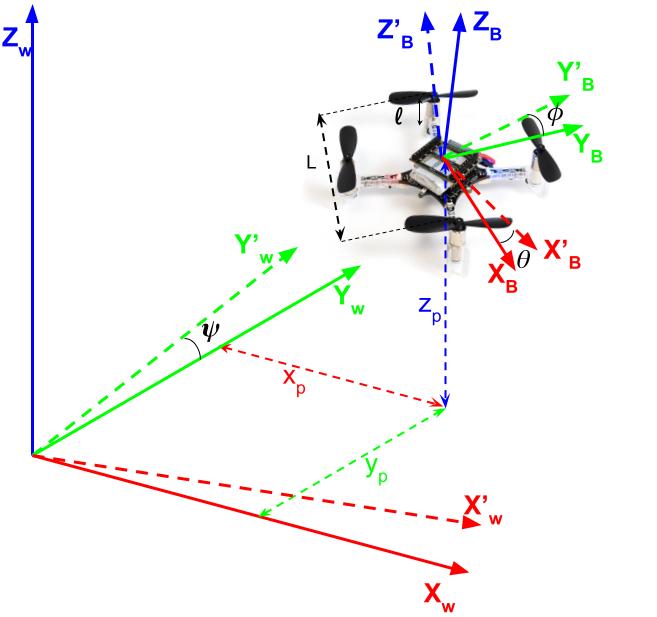
Figure 1: World coordinates and body fixed coordinates of Crazyflie and Euler’s angles defined in these coordinates

I-A Contribution and Paper Structure

Main idea is to realize a CBF-QP formulation for the quadrotor dynamics and for obstacles with non-zero velocity values. Main contributions of our work are:

• We formulate a direct method for safe trajectory tracking of quadrotors based on collision cone control barrier functions expressed through a quadratic program.

• We consider static and constant velocity obstacles of various dimensions and provide mathematical guarantees for collision avoidance.

• We compare the collision cone CBF with the state-of-the-art higher-order CBF (HO-CBF), and show how the former is better in terms of feasibility and safety guarantees.

I-B Organisation

The rest of this paper is organized as follows. Preliminaries explaining the quadrotor model, the concept of control barrier functions (CBFs), collision cone CBFs and controller design are introduced in section II. The application of the above CBFs on the quadrotor to avoid obstacles of various shapes is discussed in section III. The Simulation setup and results will be discussed in section IV. Finally, we present our conclusion in section V.

II Preliminaries

In this section, first, we will describe the dynamics of quadrotor and trajectory tracking controller. Next, we will formally introduce Control Barrier Functions (CBFs) and their importance for real-time safety-critical control. Finally, we will introduce Collision Cone CBF approach.

II-A Quadrotor model

The quadrotor model has four propellers, which provides upward thrusts of $(f_{1},f_{2},f_{3},f_{4})$ (see Fig. 1) and the states needed to describe the quadrotor system is given by $x=[x_{p},y_{p},z_{p},\dot{x}_{p},\dot{y}_{p},\dot{z}_{p},\phi,\theta,\psi,{\omega}_{1},{\omega}_{2},{\omega}_{3}]$ . The quadrotor dynamics is as follows:

$$\underbrace{\begin{bmatrix}\dot{x}_{p}\\ \dot{y}_{p}\\ \dot{z}_{p}\\ \ddot{x}_{p}\\ \ddot{y}_{p}\\ \ddot{z}_{p}\\ \dot{\phi}\\ \dot{\theta}\\ \dot{\psi}\\ \dot{\omega}_{1}\\ \dot{\omega}_{2}\\ \dot{\omega}_{3}\end{bmatrix}}_{\dot{x}}=\underbrace{\begin{bmatrix}\dot{x}_{p}\\ \dot{y}_{p}\\ \dot{z}_{p}\\ 0\\ 0\\ -g\\ \textbf{W}^{-1}\begin{bmatrix}\omega_{1}\\ \omega_{2}\\ \omega_{3}\end{bmatrix}\\ \\ -I^{-1}\vec{\omega}\times I\vec{\omega}\\ .\end{bmatrix}}_{f(x)}+\underbrace{\begin{bmatrix}\\ \begin{bmatrix}0&0&0&0\\ 0&0&0&0\\ 0&0&0&0\end{bmatrix}\\ \\ \frac{1}{m_{Q}}\textbf{R}\begin{bmatrix}0&0&0&0\\ 0&0&0&0\\ 1&1&1&1\end{bmatrix}\\ \\ \begin{bmatrix}0&0&0&0\\ 0&0&0&0\\ 0&0&0&0\end{bmatrix}\\ \\ I^{-1}L\begin{bmatrix}1&0&-1&0\\ 0&1&0&-1\\ 1&-1&1&-1\end{bmatrix}\end{bmatrix}}_{g(x)}\underbrace{\begin{bmatrix}f_{1}\\ f_{2}\\ f_{3}\\ f_{4}\end{bmatrix}}_{u}$$ (1)

$x_{p}$, $y_{p}$ and $z_{p}$ denote the coordinates of the vehicle’s centre of the base of the quadrotor in an inertial frame. $\phi$, $\theta$ and $\psi$ represents the (roll, pitch & yaw) orientation of the quadrotor. (see Fig. 1). R is the rotation matrix (from the body frame to the inertial frame), $m_{Q}$ is the mass of the quadrotor, W is the transformation matrix for angular velocities from the inertial frame to the body frame, I is the inertia matrix and L is the diagonal length of quadrotor. Note that eventhough we restrict our study to quadrotors in this paper, extension of the proposed CBF-QPs for different multi-rotor UAVs is straightforward.

II-B Trajectory tracking controller

We have to design a controller that tracks a desired trajectory with a safety filter, which modifies the input in a minimal way around the obstacles. We use a PD controller to generate a desired controller ($u_{des}$), which tracks the desired trajectory. The PD controller formulated for the quadrotor is given as follows:

$$\begin{bmatrix}\ddot{x}\\ \ddot{y}\\ \ddot{z}\end{bmatrix}:=\left(\begin{bmatrix}\ddot{x_{d}}\\ \ddot{y_{d}}\\ \ddot{z_{d}}\end{bmatrix}+\begin{bmatrix}K_{xd}(\dot{x_{d}}-\dot{x})\\ K_{yd}(\dot{y_{d}}-\dot{y})\\ K_{zd}(\dot{z_{d}}-\dot{z})\end{bmatrix}+\begin{bmatrix}K_{xp}(x_{d}-x)\\ K_{yp}(y_{d}-y)\\ K_{zp}(z_{d}-z)\end{bmatrix}\right)$$

$$\begin{bmatrix}\ddot{r}\\ \ddot{p}\end{bmatrix}:=\left(\begin{bmatrix}K_{rd}(\dot{r_{d}}-\dot{r})\\ K_{pd}(\dot{p_{d}}-\dot{p})\end{bmatrix}+\begin{bmatrix}K_{rp}(r_{d}-r)\\ K_{pp}(p_{d}-p)\end{bmatrix}\right)$$

where, $r_{d}=-\frac{\ddot{y}}{g+\ddot{z}},p_{d}=\frac{\ddot{x}}{g+\ddot{z}}$

$$\begin{bmatrix}f_{1}\\ f_{2}\\ f_{3}\\ f_{4}\end{bmatrix}:=\begin{bmatrix}1&1&1&1\\ 0&1&0&-1\\ 1&0&-1&0\\ 1&-1&1&-1\end{bmatrix}^{-1}\begin{bmatrix}m\sqrt{(\ddot{x}^{2}+\ddot{y}^{2}+(g+\ddot{z})^{2})}\\ I_{xx}\ddot{r}/L\\ -I_{xx}\ddot{p}/L\\ 0\end{bmatrix}$$

where, $K_{p}^{\prime}s$ and $K_{d}^{\prime}s$ are the proportional and derivative coefficients of respective variables.

II-C Control barrier functions (CBFs)

Having described the vehicle models, we now formally introduce Control Barrier Functions (CBFs) and their applications in the context of safety. Given the quadrotor model, we have the nonlinear control system in affine form:

$$\dot{x}=f(x)+g(x)u$$ (2)

where $x\in\mathcal{D}\subseteq\mathbb{R}^{n}$ is the state of system, and $u\in\mathbb{U}\subseteq\mathbb{R}^{m}$ the input for the system. Assume that the functions $f:\mathbb{R}^{n}\rightarrow\mathbb{R}^{n}$ and $g:\mathbb{R}^{n}\rightarrow\mathbb{R}^{n\times m}$ are continuously differentiable. Specific formulation of $f,g$ for the quadrotor were described in (1). Given a Lipschitz continuous control law $u=k(x)$, the resulting closed loop system $\dot{x}=f_{cl}(x)=f(x)+g(x)k(x)$ yields a solution $x(t)$, with initial condition $x(0)=x_{0}$. Consider a set $\mathcal{C}$ defined as the super-level set of a continuously differentiable function $h:\mathcal{D}\subseteq\mathbb{R}^{n}\rightarrow\mathbb{R}$ yielding,

$$\mathcal{C} =\{x\in\mathcal{D}\subset\mathbb{R}^{n}:h(x)\geq 0\}$$ (3)

$$\partial\mathcal{C} =\{x\in\mathcal{D}\subset\mathbb{R}^{n}:h(x)=0\}$$ (4)

$$\text{Int}\left(\mathcal{C}\right) =\{x\in\mathcal{D}\subset\mathbb{R}^{n}:h(x)>0\}$$ (5)

It is assumed that $\text{Int}\left(\mathcal{C}\right)$ is non-empty and $\mathcal{C}$ has no isolated points, i.e. $\text{Int}\left(\mathcal{C}\right)\neq\phi$ and $\overline{\text{Int}\left(\mathcal{C}\right)}=\mathcal{C}$. The system is safe w.r.t. the control law $u=k(x)$ if $\forall\>x(0)\in\mathcal{C}\implies x(t)\in\mathcal{C}\;\;\;\forall t\geq 0$. We can mathematically verify if the controller $k(x)$ is safeguarding or not by using Control Barrier Functions (CBFs), which is defined next.

Definition 1 (Control barrier function (CBF))

Given the set $\mathcal{C}$ defined by (3)-(5), with $\frac{\partial h}{\partial x}(x)\neq 0\;\forall x\in\partial\mathcal{C}$, the function $h$ is called the control barrier function (CBF) defined on the set $\mathcal{D}$, if there exists an extended class $\mathcal{K}$ function $\kappa$ such that for all $x\in\mathcal{D}$:

$$\underbrace{\text{sup}}_{u\in\mathbb{U}}\!\left[\underbrace{\mathcal{L}_{f}h(x)+\mathcal{L}_{g}h(x)u}_{\dot{h}\left(x,u\right)}\!+\kappa\left(h(x)\right)\right]\!\geq\!0$$ (6)

where $\mathcal{L}_{f}h(x)=\frac{\partial h}{\partial x}f(x)$ and $\mathcal{L}_{g}h(x)=\frac{\partial h}{\partial x}g(x)$ are the Lie derivatives. $\kappa:[0,\infty)\to[0,\infty)$ a strictly increasing continuous function with $\kappa(0)=0$. Formally, $\kappa$ is known as a class $\mathcal{K}$ function.

Given this definition of a CBF, we know from [7] and [17] that any Lipschitz continuous control law $k(x)$ satisfying the inequality: $\dot{h}+\kappa(h)\geq 0$ ensures safety of $\mathcal{C}$ if $x(0)\in\mathcal{C}$, and asymptotic convergence to $\mathcal{C}$ if $x(0)$ is outside of $\mathcal{C}$.

II-D Safety Filter Design

Having describe the CBF, we can now describe the Quadratic Programming (QP) formulation of CBFs. CBFs act as safety filters which take the desired input $u_{des}(x,t)$ and modify this input in a minimal way:

$$u^{*}(x,t) =\min_{u\in\mathbb{U}\subseteq\mathbb{R}^{m}}\left\lVert u-u_{des}(x,t)\right\rVert^{2}$$ (7)

$$\textrm{s.t. }\mathcal{L}_{f}h(x)+\mathcal{L}_{g}h(x)u+\kappa\left(h(x)\right)\geq 0$$

This is called the Control Barrier Function based Quadratic Program (CBF-QP). The CBF-QP control $u^{*}$ can be obtained by solving the above optimization problem using KKT conditions.

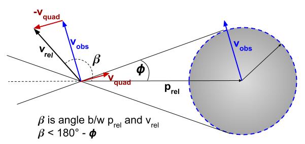
(a)

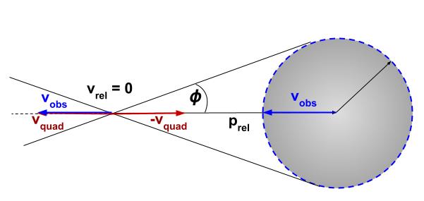
(b)

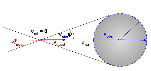
(c)

Figure 2: Construction of collision cone for an elliptical obstacle considering the quadrotor’s dimensions (width: $w$).

II-E Collision Cone CBF (C3BF) candidate for quadrotors

We now formally introduce the proposed CBF candidate for quadrotors. Let us assume that the obstacle is centered at $(c_{x}(t),c_{y}(t),c_{z}(t))$ and with dimensions $c_{1},c_{2},c_{3}$. We assume that $c_{x}(t),c_{y}(t),c_{z}(t)$ are differentiable and their derivatives are piece-wise constants. The proposed approach combines the idea of potential unsafe directions given by collision cone (Fig. 2) as unsafe set to formulate a CBF as in [16]. Consider the following CBF candidate:

$$h(x,t)=<p_{\rm{rel}},v_{\rm{rel}}>+\|p_{\rm{rel}}\|\|v_{\rm{rel}}\|\cos\phi,$$ (8)

where $p_{\rm{rel}}$ is the relative position vector between the body center of the quadrotor and the center of the obstacle, $v_{\rm{rel}}$ is the relative velocity and $\phi$ is the half angle of the cone, the expression of $\cos\phi$ is given by $\frac{\sqrt{\|p_{\rm{rel}}\|^{2}-r^{2}}}{\|p_{\rm{rel}}\|}$ (see Fig. 3, 4). Precise mathematical definitions for $p_{\rm{rel}},v_{\rm{rel}}$ will be given in the next section. The proposed constraint simply ensures that the angle between $p_{\rm{rel}},v_{\rm{rel}}$ is less than $180^{\circ}-\phi$.

In [16], it was shown that the proposed candidate (8) is valid CBF for wheeled mobile robots, i.e., the unicycle and bicycle. With this result, CBF-QPs were constructed that yielded collision avoiding behaviors in these models. We aim to extend this for the class of quadrotors.

III Collision Cone CBFs on Quadrotor

Having described Collision Cone CBF candidate, we will see their application on quadrotor in this section. Based on the shape of the obstacle we can divide the proposed candidates into two cases:

III-1 3D CBF candidate

When the dimensions of the obstacle are comparable to each other, we can assume the obstacle as a sphere with radius $r=max(c_{1},c_{2},c_{3})+\frac{w}{2}$, where $w$ is the max width of the quadrotor absorbed in the obstacle width (shown in Fig. 3). We call the CBF candidate so formed in this case as 3D CBF candidate (see Fig. 3).

III-2 Projection CBF candidate

When one of the dimensions is far bigger than the other dimensions, we can assume the obstacle as a cylinder with height $H=max(c_{1},c_{2},c_{3})$ and radius $r=max_{2}(c_{1},c_{2},c_{3})+\frac{w}{2}$ (where $max_{2}$ is the second largest element in the list) and we call the candidate so formed in this case as Projection CBF candidate (see Fig. 4).

III-A 3D CBF candidate

We first obtain the relative position vector between the body center of the quadrotor and the center of the obstacle. We have the following:

$$p_{\rm{rel}}:=\begin{bmatrix}c_{x}\\ c_{y}\\ c_{z}\end{bmatrix}-\left(\begin{bmatrix}x_{p}\\ y_{p}\\ z_{p}\end{bmatrix}+\textbf{R}\begin{bmatrix}0\\ 0\\ l\end{bmatrix}\right)$$ (9)

Here $l$ is the distance of the body center from the base (see Fig. 1). $c_{x},c_{y},c_{z}$ represents the obstacle location as a function of time. Also, since the obstacles are of constant velocity, we have $\ddot{c}_{x}=\ddot{c}_{y}=\ddot{c}_{z}=0$. We obtain its relative velocity as

$$v_{\rm{rel}}:=\dot{p}_{rel}$$ (10)

Now, we calculate the $\dot{v}_{\rm{rel}}$ term which contains our inputs i.e. $(f_{1},f_{2},f_{3},f_{4})$, as follows:

$$\dot{v}_{\rm{rel}}=-\textbf{R}\begin{bmatrix}0&\frac{Ll}{I_{yy}}&0&\frac{-Ll}{I_{yy}}\\ \frac{-Ll}{I_{xx}}&0&\frac{Ll}{I_{xx}}&0\\ \frac{1}{m}&\frac{1}{m}&\frac{1}{m}&\frac{1}{m}\end{bmatrix}\begin{bmatrix}f_{1}\\ f_{2}\\ f_{3}\\ f_{4}\end{bmatrix}\\ +\rm{additional}\>\rm{terms}.$$

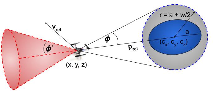
Figure 3: 3D CBF candidate: The dimensions of the obstacle are comparable to each other, it can be assumed as a sphere

Having introduced Collision Cone CBF candidates in II-E, the next step is to formally verify that they are, indeed, valid CBFs. We have the following result.

Theorem 1

Given the quadrotor model (1), the proposed CBF candidate (8) with $p_{\rm{rel}},v_{\rm{rel}}$ defined by (9), (10) is a valid CBF defined for the set $\mathcal{D}$.

Proof:

Since we are considering the 3D case, we will denote the resulting CBF candidate given by (8) by $h_{3D}$. We have the following derivative:

$$\dot{h}_{3D}= <\dot{p}_{\rm{rel}},v_{\rm{rel}}>+<p_{\rm{rel}},\dot{v}_{\rm{rel}}>$$

$$+<v_{\rm{rel}},\dot{v}_{\rm{rel}}>\frac{\sqrt{\|p_{\rm{rel}}\|^{2}-r^{2}}}{\|v_{\rm{rel}}\|}$$

$$+<p_{\rm{rel}},\dot{p}_{\rm{rel}}>\frac{\|v_{\rm{rel}}\|}{\sqrt{\|p_{\rm{rel}}\|^{2}-r^{2}}}.$$ (11)

By substituting for $\dot{v}_{\rm{rel}}$ (which contains the input) in $\dot{h}_{3D}$ (11), we have the following expression for $\mathcal{L}_{g}h_{3D}$:

$$\mathcal{L}_{g}h_{3D}=\begin{bmatrix}<p_{\rm{rel}}+v_{\rm{rel}}\frac{\sqrt{\|p_{\rm{rel}}\|^{2}-r^{2}}}{\|v_{\rm{rel}}\|},\textbf{R}\begin{bmatrix}0\\ \frac{-Ll}{I_{xx}}\\ \frac{1}{m}\end{bmatrix}>\\ <p_{\rm{rel}}+v_{\rm{rel}}\frac{\sqrt{\|v_{\rm{rel}}\|^{2}-r^{2}}}{\|v_{\rm{rel}}\|},\textbf{R}\begin{bmatrix}\frac{Ll}{I_{yy}}\\ 0\\ \frac{1}{m}\end{bmatrix}>\\ <p_{\rm{rel}}+v_{\rm{rel}}\frac{\sqrt{\|v_{\rm{rel}}\|^{2}-r^{2}}}{\|v_{\rm{rel}}\|},\textbf{R}\begin{bmatrix}0\\ \frac{Ll}{I_{xx}}\\ \frac{1}{m}\end{bmatrix}>\\ <p_{\rm{rel}}+v_{\rm{rel}}\frac{\sqrt{\|v_{\rm{rel}}\|^{2}-r^{2}}}{\|v_{\rm{rel}}\|},\textbf{R}\begin{bmatrix}\frac{-Ll}{I_{yy}}\\ 0\\ \frac{1}{m}\end{bmatrix}>\end{bmatrix}^{T},$$ (12)

It can be verified that for $\mathcal{L}_{g}h_{3D}$ to be zero, we can have the following scenarios:

• $p_{\rm{rel}}+v_{\rm{rel}}\frac{\sqrt{\|p_{\rm{rel}}\|^{2}-r^{2}}}{\|v_{\rm{rel}}\|}=0$, which is not possible. Firstly, $p_{\rm{rel}}=0$ indicates that the vehicle is already inside the obstacle. Secondly, if the above equation were to be true for a non-zero $p_{\rm{rel}}$, then $v_{\rm{rel}}/\|v_{\rm{rel}}\|=-p_{\rm{rel}}/\sqrt{\|p_{\rm{rel}}\|^{2}-r^{2}}$. This is also not possible as the magnitude of LHS is $1$, while that of RHS is $>1$.

• $p_{\rm{rel}}+v_{\rm{rel}}\frac{\sqrt{\|v_{\rm{rel}}\|^{2}-r^{2}}}{\|v_{\rm{rel}}\|}$ is perpendicular to all $\textbf{R}\begin{bmatrix}0\\ \frac{-Ll}{I_{xx}}\\ \frac{1}{m}\end{bmatrix}$, $\textbf{R}\begin{bmatrix}\frac{Ll}{I_{yy}}\\ 0\\ \frac{1}{m}\end{bmatrix}$, $\textbf{R}\begin{bmatrix}0\\ \frac{Ll}{I_{xx}}\\ \frac{1}{m}\end{bmatrix}$ and $\textbf{R}\begin{bmatrix}\frac{-Ll}{I_{yy}}\\ 0\\ \frac{1}{m}\end{bmatrix}$, which is also not possible. (Because three of these vectors form basis vectors for $\mathbb{R}^{3}$)

This implies that $\mathcal{L}_{g}h_{3D}$ is always a non-zero matrix, implying that $h_{3D}$ is a valid CBF. ∎

III-B Projection CBF candidate

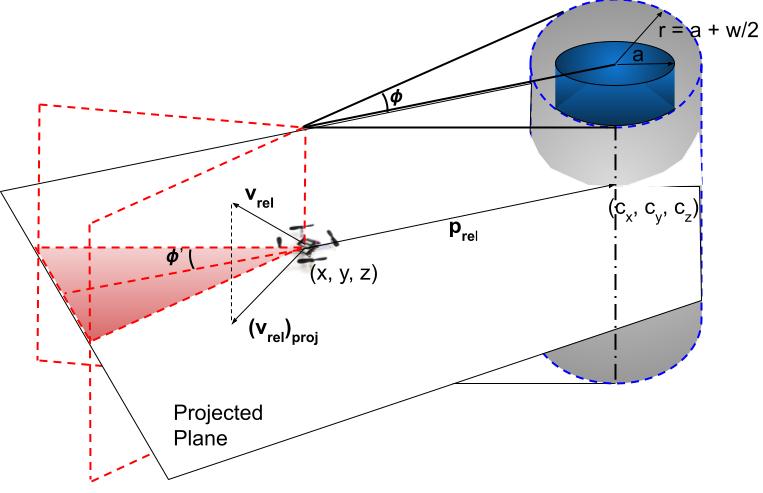
Figure 4: Projection CBF candidate: One of the dimensions, of the obstacle, is bigger than the other dimensions, it can be assumed as a cylinder.

Now, we have to consider the collision avoidance for elongated (cylindrical) obstacles. We have to obtain the relative position vector between the body center of the quadrotor and the intersection of the axis of the obstacle and the projection plane, where the projection plane is the plane perpendicular to the axis. Therefore, we have

$$(p_{\rm{rel}})_{proj}:=\mathcal{P}\left(\begin{bmatrix}c_{x}\\ c_{y}\\ c_{z}\end{bmatrix}-\left(\begin{bmatrix}x_{p}\\ y_{p}\\ z_{p}\end{bmatrix}+\textbf{R}\begin{bmatrix}0\\ 0\\ l\end{bmatrix}\right)\right).$$ (13)

Here $l$ is the distance of the body center from the base (see Fig. 1). $\mathcal{P}:\mathbb{R}^{3}\to\mathbb{R}^{3}$ is the projection operator, which can be assumed to be a constant. Now, since the relative position lies on the projection plane, we have one more condition to satisfy:

$$<(p_{\rm{rel}})_{proj},\hat{n}>=0,$$ (14)

where, $\hat{n}$ is the normal to the plane. Also, the relative velocity is given by:

$$(v_{\rm{rel}})_{proj}:=\frac{d({p}_{rel})_{proj}}{dt}=(\dot{p}_{\rm{rel}})_{proj}$$ (15)

Now, we calculate the $\frac{d}{dt}(v_{\rm{rel}})_{proj}$ term which contains our inputs i.e. $(f_{1},f_{2},f_{3},f_{4})$, as follows:

$$\frac{d}{dt}(v_{\rm{rel}})_{proj}=\mathcal{P}(-\textbf{R}\begin{bmatrix}0&\frac{Ll}{I_{yy}}&0&\frac{-Ll}{I_{yy}}\\ \frac{-Ll}{I_{xx}}&0&\frac{Ll}{I_{xx}}&0\\ \frac{1}{m}&\frac{1}{m}&\frac{1}{m}&\frac{1}{m}\end{bmatrix}\begin{bmatrix}f_{1}\\ f_{2}\\ f_{3}\\ f_{4}\end{bmatrix}\\ +\rm{additional}\>\rm{terms}).$$

or, from (III-A), we have

$$\frac{d}{dt}(v_{\rm{rel}})_{proj}=\mathcal{P}(\dot{v}_{\rm{rel}})$$ (16)

$\frac{d}{dt}(v_{\rm{rel}})_{proj}$ is the projection of $\dot{v}_{\rm{rel}}$ in (III-A) on the projection plane, that is:

$$(\dot{v}_{\rm{rel}})_{proj}=\dot{v}_{\rm{rel}}-<\dot{v}_{\rm{rel}},\hat{n}>\hat{n}.$$ (17)

Thus, from (14) and (17), we have the following:

$$<(p_{\rm{rel}})_{proj},(\dot{v}_{\rm{rel}})_{proj}>=<(p_{\rm{rel}})_{proj},\dot{v}_{\rm{rel}}>.$$ (18)

Similarly,

$$<(v_{\rm{rel}})_{proj},(\dot{v}_{\rm{rel}})_{proj}>=<(v_{\rm{rel}})_{proj},\dot{v}_{\rm{rel}}>$$ (19)

We now provide the formal results for (8) for the Projection case in this subsection. The candidate is given as follows:

$$h_{proj}(x,t)=<(p_{\rm{rel}})_{proj},(v_{\rm{rel}})_{proj}>+\|(p_{\rm{rel}})_{proj}\|\|(v_{\rm{rel}})_{proj}\|\cos\phi$$ (20)

where, $\phi$ is the half angle of the cone, the expression of $\cos\phi$ is given by $\frac{\sqrt{\|(p_{\rm{rel}})_{proj}\|^{2}-r^{2}}}{\|(p_{\rm{rel}})_{proj}\|}$ (see Fig. 4). We now show that the proposed CBF candidate (20) is indeed a valid CBF.

Theorem 2

Given the quadrotor model (1), the proposed CBF candidate (20) with $p_{\rm{rel}},v_{\rm{rel}}$ defined by (13), (15) is a valid CBF defined for the set $\mathcal{D}$.

Proof:

We have the following derivative of $h_{proj}$:

$$\dot{h}_{proj}= <(\dot{p}_{\rm{rel}})_{proj},(v_{\rm{rel}})_{proj}>+<(p_{\rm{rel}})_{proj},(\dot{v}_{\rm{rel}})_{proj}>$$

$$+<(v_{\rm{rel}})_{proj},(\dot{v}_{\rm{rel}})_{proj}>\frac{\sqrt{\|(p_{\rm{rel}})_{proj}\|^{2}-r^{2}}}{\|(v_{\rm{rel}})_{proj}\|}$$

$$+<(p_{\rm{rel}})_{proj},(\dot{p}_{\rm{rel}})_{proj}>\frac{\|(v_{\rm{rel}})_{proj}\|}{\sqrt{\|(p_{\rm{rel}})_{proj}\|^{2}-r^{2}}}.$$ (21)

$\dot{v}_{\rm{rel}}$ (which contains the input) from (17), equations (18), (19) and $\dot{h}_{proj}$ (21), we have the following expression for $\mathcal{L}_{g}h_{proj}$:

$$\mathcal{L}_{g}h_{proj}=\begin{bmatrix}<p_{\rm{rel}}+v_{\rm{rel}}\frac{\sqrt{\|p_{\rm{rel}}\|^{2}-r^{2}}}{\|v_{\rm{rel}}\|},\textbf{R}\begin{bmatrix}0\\ \frac{-Ll}{I_{xx}}\\ \frac{1}{m}\end{bmatrix}>\\ <p_{\rm{rel}}+v_{\rm{rel}}\frac{\sqrt{\|v_{\rm{rel}}\|^{2}-r^{2}}}{\|v_{\rm{rel}}\|},\textbf{R}\begin{bmatrix}\frac{Ll}{I_{yy}}\\ 0\\ \frac{1}{m}\end{bmatrix}>\\ <p_{\rm{rel}}+v_{\rm{rel}}\frac{\sqrt{\|v_{\rm{rel}}\|^{2}-r^{2}}}{\|v_{\rm{rel}}\|},\textbf{R}\begin{bmatrix}0\\ \frac{Ll}{I_{xx}}\\ \frac{1}{m}\end{bmatrix}>\\ <p_{\rm{rel}}+v_{\rm{rel}}\frac{\sqrt{\|v_{\rm{rel}}\|^{2}-r^{2}}}{\|v_{\rm{rel}}\|},\textbf{R}\begin{bmatrix}\frac{-Ll}{I_{yy}}\\ 0\\ \frac{1}{m}\end{bmatrix}>\end{bmatrix}^{T},$$ (22)

Using the same arguments we gave in the proof of theorem. 1, we can infer that $\mathcal{L}_{g}h_{proj}$ cannot be zero. This implies that $h_{proj}$ is a valid CBF. ∎

Remark 1

Based on Theorems (1) and (2), where $\mathcal{L}_{g}h\neq 0$, we can utilize the conclusion from [18, Theorem 8] to deduce that the control inputs obtained from the resulting CBF-QP (7) are Lipschitz continuous. As a result, the resulting solutions guarantee forward invariance of the safe set generated by the proposed C3BF candidates.

III-C Comparison with Higher Order CBFs

We introduce the state-of-the-art Higher Order Control Barrier Functions (HO-CBFs) and compare with the proposed C3BF in this section. Since, the collision constraints are w.r.t. the position, the corresponding CBF is of relative degree two, we need to define a Higher Order CBF with $m=2$ as in [12, Eq 16], which is given as:

$$\psi_{1}(x,t) =\dot{b}(x,t)+p\alpha_{1}(b(x,t))$$ (23)

$$\psi_{2}(x,t) =\dot{\psi_{1}}(x,t)+p\alpha_{2}(\psi_{1}(x,t)),$$

where $b(x,t)=(c_{x}(t)-x_{p})^{2}+(c_{y}(t)-y_{p})^{2}+(c_{z}(t)-z_{p})^{2}-r^{2}$, and r is the encompassing radius given by $r=max(c_{1},c_{2},c_{3})$. $\alpha_{1},\alpha_{2}$ are both class $\mathcal{K}$ functions, and $p$ is a tunable constant. As explained previously, $c_{x},c_{y},c_{z}$ is the centre location of the obstacle as a function of time. Let us examine the form of HO-CBF where $\alpha_{1}$ is a square root function (which is also strictly increasing), $\alpha_{2}$ is a linear function, due to its similarity to C3BF. Consequently, the resulting Higher Order CBF candidate takes the following form:

$$h_{HO}(x,t)=<p_{\rm{rel}},v_{\rm{rel}}>+\gamma\sqrt{(\|p_{\rm{rel}}\|^{2}-r^{2})}.$$ (24)

We can show that the above mentioned HO-CBF is also a valid CBF as we did in Theorems 1 and 2. We will now compare it with the proposed C3BF.

The C3BF concept aims to prevent the $v_{\rm{rel}}$ vector, which represents the relative velocity between the quadrotor and the obstacle, from entering the collision cone region defined by the half-angle $\phi$. Figures 3, 4 and 5 illustrate this idea. We can rewrite the HO-CBF formula presented in (24) in the following form:

$$h_{HO}(x,t)=<p_{\rm{rel}},v_{\rm{rel}}>+\|p_{\rm{rel}}\|\|v_{\rm{rel}}\|cos(\phi^{\prime})$$ (25)

where, $cos(\phi^{\prime})=\frac{\gamma}{\|v_{\rm{rel}}\|}cos(\phi)$. If we are able to identify a suitable $\gamma$ (penalty term) for the given HO-CBF, it would result in a valid CBF as per [12]. Nonetheless, in such a scenario where $\gamma$ remains constant and $\|v_{\rm{rel}}\|$ goes on increasing, it leads to increase in $\phi^{\prime}$, thus, overestimating the cone as can be seen in Fig.5. Conversely, with the C3BF approach, we permit the penalty term to vary over time, i.e., $\gamma=\|v_{\rm{rel}}\|$, resulting in a more precise estimation of the collision cone compared to the HO-CBF case. This also shows that C3BF is not a special case of Higher Order CBF. This is also evident from the simulation outcomes of both CBFs, as demonstrated in Section IV.

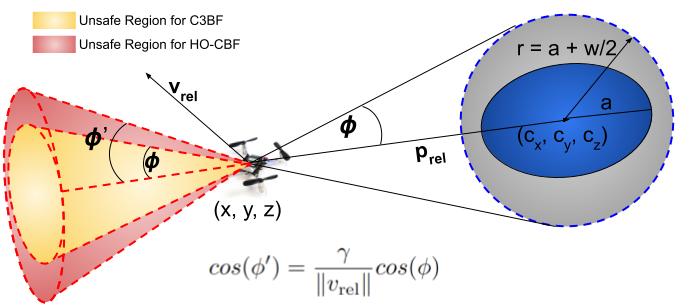
Figure 5: Comparison of HO-CBF with C3BF. Here we are trying to compare the $\phi^{\prime}$ and $\phi$ obtained from the two CBF formulations. It can be observed that $\phi^{\prime}$ (pink cone) is dependent on $v_{rel}$, while $\phi$ (yellow cone) is a constant. The HO-CBF guarantees safety for a set that is not only smaller but also dependent on $v_{rel}$ as shown by the pink cone. Hence, HO-CBF is more conservative compared to C3BF.

IV Simulation Results

We have validated the C3BF-QP based controller on quadrotors for both 3D and Projection CBF cases. The simulations were conducted using the multi-drone environment [19] on Pybullet [20], a python-based physics simulation engine. The parameters of Crazyflie are tabulated in I. PD Controller is used as a reference controller to track the desired path, and the safety controller deployed is given by Sections II-B II-D. We chose constant target velocities for verifying the C3BF-QP. For the class $\mathcal{K}$ function in the CBF inequality, we chose $\kappa(h)=\gamma h$, where $\gamma=1$.

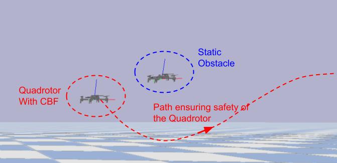
(a)

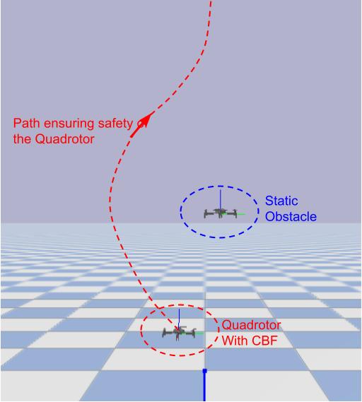
(b)

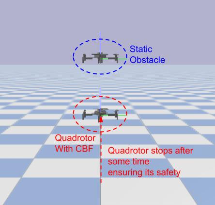
(c)

Figure 6: Interaction with static obstacles: overtaking (a), (b), and braking (c) behavior of the quadrotor, Section III-A.

Variables	Definition	Value
g	Gravitational acceleration	$9.81kg\cdot m/s^{2}$
m	Mass of quadrotor	$0.027kg$
L	Distance between two opp. rotors	0.130 $m$
l	Distance of center from base	$0.014m$
Ix, Iy	Inertia about x, y-axis	$2.39\cdot 10^{-5}kg\cdot m^{2}$
Iz	Inertia about z-axis	$3.23\cdot 10^{-5}kg\cdot m^{2}$
kf	Motor’s thrust constant	$3.16\cdot 10^{-10}$
km	Motor’s torque constant	$7.94\cdot 10^{-12}$

TABLE I: Modelling parameters of Crazyflie

IV-A Simulation setup

Having presented our proposed control method design, we now test our framework under three different scenarios to illustrate the performance of the controller. These scenarios include the interaction of quadrotor with: (1) a static obstacle (3D case) Fig. 6, (2) a moving obstacle (3D case) Fig. 7 and (3) an elongated obstacle (Projection case) Fig. 8.

IV-A1 Interaction with static obstacles

Fig. 6 shows the overtaking (a, b), and braking (c) behavior of the quadrotor while interacting with the static obstacle (which is another quadrotor). In all these cases the reference velocity of the quadrotor is 1m/s.

IV-A2 Interaction with moving obstacles

Fig. 7 shows the overtaking (a), (b), slowing (c), and reversing (d) behavior of the quadrotor while interacting with the moving obstacle (which is another quadrotor). In all these cases the reference velocity of the quadrotor is 1m/s and the obstacle quadrotor speed is 1m/s in case (a) and 0.1 m/s in (b),(c),(d).

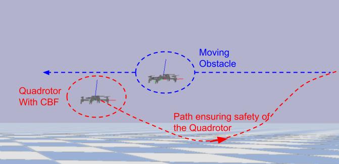
(a)

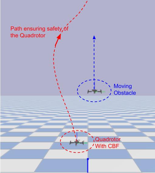
(b)

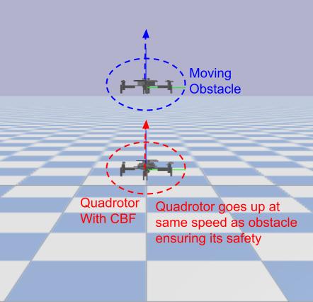
(c)

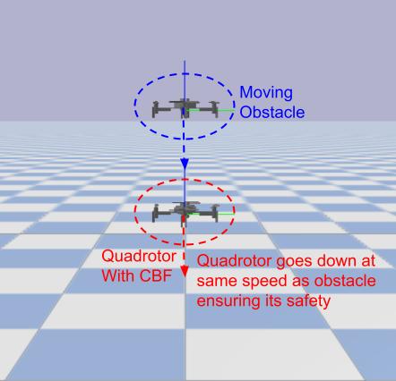
(d)

Figure 7: Interaction with moving obstacles: overtaking (a), (b), slowing (c), and reversing (d) behavior of the quadrotor, section III-A

IV-A3 Interaction with long obstacles

Fig. 8 shows the quadrotor moving from side and top in (a), (b) respectively while interacting with an elongated obstacle. In all these cases the reference velocity of the quadrotor is 1m/s.

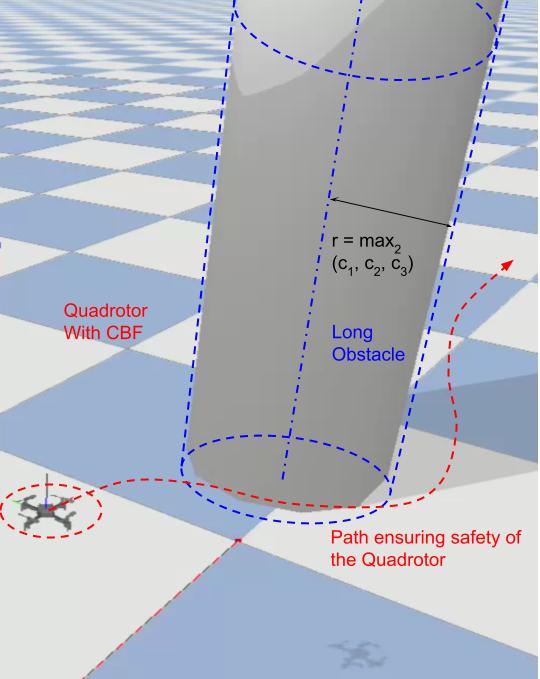
(a)

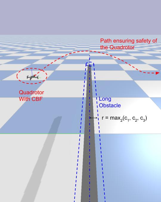
(b)

Figure 8: Interaction with longer obstacles: moving from side (a) and top (b), Section III-B.

IV-B Comparison between C3BF and HO-CBF

All the aforementioned cases were tested with the HO-CBF to compare its performance against C3BF. We observe that the HO-CBF could not avoid a high-speed approaching obstacle. Moreover, it is not able to properly avoid the longer obstacles in the projection CBF case. These shortcomings of the Higher Order CBF are demonstrated in the supplementary video.

IV-C Robustness of C3BF

Without changing the above control framework we can observe that the C3BF is robust in the following two cases:

IV-C1 Multiple Obstacles

We have considered the scenario where the quadrotor is made to move through a series of obstacles (both Spherical and Long obstacles) as in Fig. 9 (a) & (b). We observe that the quadrotor is able to successfully navigate through this complex environment by avoiding all the obstacles, thus demonstrating robustness with respect to multiple obstacles.

IV-C2 Multiple quadrotors with C3BF-QPs

We have also considered the multi-agent scenarios where the multiple quadrotors have the collision cone CBF-QP operational as shown in Fig. 9 (c). We observe that both the ego-quadrotor and the approaching quadrotor are able to avoid collision in different configurations (static or moving), thus demonstrating robustness with respect to obstacles following the same Collision Cone CBF controller.

The supplementary video shows the simulation video of all the scenarios shown in Fig 9.

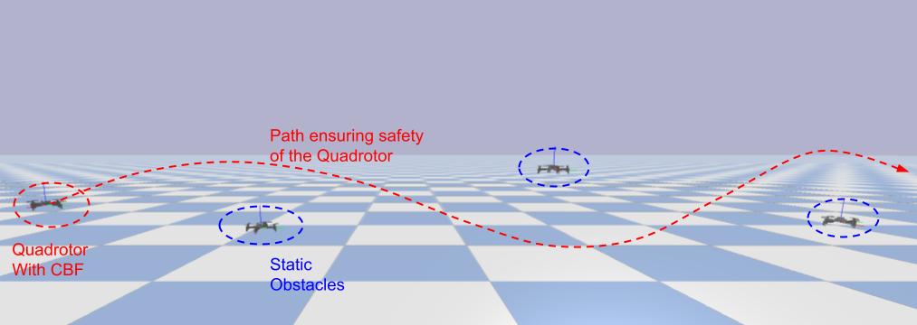
(a)

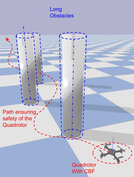
(b)

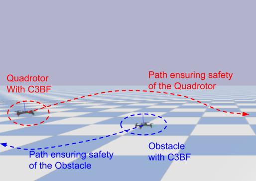
(c)

Figure 9: Robustness in scenarios with multiple obstacles (a), (b) and with obstacle also following Collision Cone CBF(c).

V Conclusions

We presented the extension of a novel collision cone CBF formulation for quadrotors to avoid collision with moving obstacles of various shapes and sizes. We successfully constructed CBF-QPs with the proposed CBF for the quadrotor model and guarantee safety by avoiding moving obstacles. This includes collision avoidance with spherical and cylindrical obstacles. We also showed that the current state-of-the-art Higher Order CBFs is more conservative and fails in certain scenarios (shown in video). Finally, we demonstrated the robustness of the proposed CBF-QP controller with respect to safe navigation in a cluttered environment consisting of multiple obstacles and agents with the same safety filters. In our future work, we plan to implement the controller on quadrotors in real-world situations, interacting with a variety of obstacles. We also intend to explore applications such as safe tele-operation of quadrotors. Additionally, we aim to investigate the potential of applying the C3BF formulation to legged robots walking in confined spaces.

References

- [1] V. Kumar, “The future of flying robots,” TED Talk, 2015.
- [2] J. Sun, J. Tang, and S. Lao, “Collision avoidance for cooperative uavs with optimized artificial potential field algorithm,” IEEE Access, vol. 5, pp. 18 382–18 390, 2017.
- [3] S. Bansal, M. Chen, S. Herbert, and C. J. Tomlin, “Hamilton-jacobi reachability: A brief overview and recent advances,” in 2017 IEEE 56th Annual Conference on Decision and Control (CDC), 2017, pp. 2242–2253.
- [4] Y. Lin and S. Saripalli, “Collision avoidance for uavs using reachable sets,” in 2015 International Conference on Unmanned Aircraft Systems (ICUAS), 2015, pp. 226–235.
- [5] M. Castillo-Lopez, S. A. Sajadi-Alamdari, J. L. Sanchez-Lopez, M. A. Olivares-Mendez, and H. Voos, “Model predictive control for aerial collision avoidance in dynamic environments,” in 2018 26th Mediterranean Conference on Control and Automation (MED), 2018, pp. 1–6.
- [6] A. D. Ames, J. W. Grizzle, and P. Tabuada, “Control barrier function based quadratic programs with application to adaptive cruise control,” in 53rd IEEE Conference on Decision and Control, 2014, pp. 6271–6278.
- [7] A. D. Ames, X. Xu, J. W. Grizzle, and P. Tabuada, “Control barrier function based quadratic programs for safety critical systems,” IEEE Transactions on Automatic Control, vol. 62, no. 8, pp. 3861–3876, aug 2017. [Online]. Available: https://doi.org/10.1109%2Ftac.2016.2638961
- [8] Z. Li, “Comparison between safety methods control barrier function vs. reachability analysis,” 2021. [Online]. Available: https://arxiv.org/abs/2106.13176
- [9] A. W. Singletary, K. Klingebiel, J. R. Bourne, N. A. Browning, P. T. Tokumaru, and A. D. Ames, “Comparative analysis of control barrier functions and artificial potential fields for obstacle avoidance,” 2021 IEEE/RSJ International Conference on Intelligent Robots and Systems (IROS), pp. 8129–8136, 2021.
- [10] G. Wu and K. Sreenath, “Safety-critical control of a planar quadrotor,” in 2016 American Control Conference (ACC), 2016, pp. 2252–2258.
- [11] W. Xiao and C. Belta, “Control barrier functions for systems with high relative degree,” CoRR, vol. abs/1903.04706, 2019. [Online]. Available: http://arxiv.org/abs/1903.04706
- [12] ——, “High-order control barrier functions,” IEEE Transactions on Automatic Control, vol. 67, no. 7, pp. 3655–3662, 2022.
- [13] P. Fiorini and Z. Shiller, “Motion planning in dynamic environments using the relative velocity paradigm,” in [1993] Proceedings IEEE International Conference on Robotics and Automation, 1993, pp. 560–565 vol.1.
- [14] ——, “Motion planning in dynamic environments using velocity obstacles,” The International Journal of Robotics Research, vol. 17, no. 7, pp. 760–772, 1998. [Online]. Available: https://doi.org/10.1177/027836499801700706
- [15] A. Chakravarthy and D. Ghose, “Obstacle avoidance in a dynamic environment: a collision cone approach,” IEEE Transactions on Systems, Man, and Cybernetics - Part A: Systems and Humans, vol. 28, no. 5, pp. 562–574, 1998.
- [16] P. Thontepu, B. G. Goswami, N. Singh, S. P, S. S. M. G, S. Sundaram, V. Katewa, and S. Kolathaya., “Control barrier functions in ugvs for kinematic obstacle avoidance: A collision cone approach,” 2022. [Online]. Available: https://arxiv.org/abs/2209.11524
- [17] A. D. Ames, S. Coogan, M. Egerstedt, G. Notomista, K. Sreenath, and P. Tabuada, “Control barrier functions: Theory and applications,” in 2019 18th European Control Conference (ECC), 2019, pp. 3420–3431.
- [18] X. Xu, P. Tabuada, J. W. Grizzle, and A. D. Ames, “Robustness of control barrier functions for safety critical control.” IFAC-PapersOnLine, vol. 48, no. 27, pp. 54–61, 2015, analysis and Design of Hybrid Systems ADHS. [Online]. Available: https://www.sciencedirect.com/science/article/pii/S2405896315024106
- [19] J. Panerati, H. Zheng, S. Zhou, J. Xu, A. Prorok, and A. P. Schoellig, “Learning to fly—a gym environment with pybullet physics for reinforcement learning of multi-agent quadcopter control,” in 2021 IEEE/RSJ International Conference on Intelligent Robots and Systems (IROS), 2021.
- [20] E. Coumans and Y. Bai, “Pybullet, a python module for physics simulation for games, robotics and machine learning,” http://pybullet.org, 2016–2019.