Automated wildlife image classification: An active learning tool for ecological applications

Abstract

Wildlife camera trap images are being used extensively to investigate animal abundance, habitat associations, and behavior, which is complicated by the fact that experts must first classify the images to retrieve relevant information. Artificial intelligence systems can take over this task but usually need a large number of already-labeled training images to achieve sufficient performance. This requirement necessitates human expert labor and poses a particular challenge for projects with few cameras or short durations. We propose a label-efficient learning strategy that enables researchers with small or medium-sized image databases to leverage the potential of modern machine learning, thus freeing crucial resources for subsequent analyses.
Our methodological proposal is two-fold: On the one hand, we improve current strategies of combining object detection and image classification by tuning the hyperparameters of both models. On the other hand, we provide an active learning system that allows training deep learning models very efficiently in terms of required manually labeled training images. We supply a software package that enables researchers to use these methods without specific programming skills and thereby ensure the broad applicability of the proposed framework in ecological practice.
We show that our tuning strategy improves predictive performance, emphasizing that tuning can and must be done separately for a new data set. We demonstrate how the active learning pipeline reduces the amount of pre-labeled data needed to achieve specific predictive performance and that it is especially valuable for improving out-of-sample predictive performance.
We conclude that the combination of tuning and active learning increases the predictive performance of automated image classifiers substantially. Furthermore, we argue that our work can broadly impact the community through the ready-to-use software package provided. Finally, the publication of our models tailored to European wildlife data enriches existing model bases mostly trained on data from Africa and North America.

^aDepartment of Statistics, LMU Munich, Ludwigstr. 33, 80539 München, Germany
^bMunich Center for Machine Learning (MCML), Ludwigstr. 33, 80539 München, Germany
^cMunich Center for Mathematical Philosophy (MCMP), Ludwigstr. 31, 80539 München, LMU Munich, Germany
^dWildlife Biology and Management Research Unit, Bavarian State Institute of Forestry (LWF), Hans-Carl-von-Carlowitz-Platz 1, 85354 Freising, Germany
^eWildlife Biology and Management Unit, Technical University of Munich, Hans-Carl-von-Carlowitz-Platz 2, 85354 Freising, Germany
^fEcoclimatology, TUM School of Life Sciences, Technical University of Munich, Hans-Carl-von-Carlowitz-Platz 2, 85354 Freising, Germany
^gTUM Institute for Advanced Study, Lichtenbergstraße 2 a 85748 Garching, Germany
^∗Corresponding author: ludwig.bothmann@stat.uni-muenchen.de

Keywords: active learning, deep learning, European animal species, hyperparameter tuning, object detection, wildlife image classification

1 Introduction

Wildlife camera traps have been increasingly used for estimating the abundance and distribution of animal communities, studying animal behavior, and assessing animal-plant interactions over the last decade [Delisle et al., 2021, Trolliet et al., 2014, Tuia et al., 2022]. Since manual annotation of large image data sets is time-consuming and expensive, machine learning (ML) techniques, especially from the field of deep learning (DL) have been developed, customized, and applied to wildlife image data sets [Auer et al., 2021, Beery et al., 2019, Christin et al., 2019, Gimenez et al., 2021, Miao et al., 2021, Norouzzadeh et al., 2018, 2021, Schneider et al., 2019, 2020, Tabak et al., 2019, 2020, 2022, Whytock et al., 2021]. These techniques allow for high detection rates in the investigated data sets.

However, the broad applicability of the proposed methods is hindered for different reasons: First, models are often trained on data sets from specific regions of the earth, e.g., the Serengeti Snapshot data from Africa [Swanson et al., 2015], the North American Camera Trap Images [Tabak et al., 2019] and Caltech Camera Traps [Beery et al., 2018] from North America, the LILA database with images from outside Europe, and DeepFaune [Rigoudy et al., 2022] from France. Applying such models to other animal species or habitats, which are not representative of the data used for model training, leads to a drop in predictive performance, see also Beery et al. [2018], Koh et al. [2021], Schneider et al. [2020], Shepley et al. [2021], Tuia et al. [2022]. Second, training such models for new animal species or new habitats demands a large amount of manually annotated training images, which may not be available for smaller research groups that operate in regions where models trained on the above-mentioned data sets result in poor classification performance. Third, highly customizable software targeted at experienced programmers may be an obstacle for applied researchers from ecology who would benefit much more from an easy-to-use software package that yields high-performing ML models across a range of tasks, see, e.g., Vélez et al. [2023], Gimenez et al. [2021].

We aim at filling this gap by proposing an active learning pipeline that yields high-performing models, demands only small training data sets, and is readily usable – via accompanying example code and tutorials – for researchers in ecology without any specific background in ML or computer science. Our main research goals are:

• achieving high out-of-sample (OOS) performance, i.e., good transferability to new domains,

• dealing with both existing and new, previously unseen animal species,

• providing solutions for small data sets ($<50.000$ images),

• adding models pre-trained on European wildlife images to the existing pre-trained models that are mainly from Africa and North America, and

• supplying highly usable software that can be used off-the-shelf at a low computational cost.

1.1 Main contributions

1.1.1 Active learning pipeline

Our pipeline consists of four main building blocks: We combine the benefits of object detection – to locate parts of an image that most likely contain animals – and image classification – to classify the animal species found by the object detector. A thorough tuning process optimizes the hyperparameters of both the object detector and image classifier, including the architecture of the deep neural network used for transfer learning. Finally, an active learning component allows training a new model or adapting a pre-trained model to new animal classes or habitats with a substantially reduced need for training data from that new domain. We will explain the central components of the pipeline in the following and refer to “Materials and Methods” for a thorough explanation of all steps.

Combining object detection and image classification

A key factor for creating a powerful pipeline is the combination of object detection and image classification, see also Curry et al. [2021]. First, using a pre-trained object detection network, as proposed, e.g., by Beery et al. [2019], allows for rapid identification of empty images [Vélez et al., 2023]. Otherwise, the task of locating empty images is either very time-consuming – Gimenez et al. [2021] mention that doing this manually “took several weeks of labor full time” for a rather small data set of $<50.000$ images – or technically complicated without yielding convincing results (e.g., Auer et al. [2021] tried to use active learning to filter out empty images). Second, image backgrounds and camera-added information (such as a header or footer) are removed and the image classifier can directly focus on the parts of the image where the object detector has detected an animal. As a result, fewer training images are necessary to adapt pre-trained models to new domains; furthermore, the number of animals on a given image can be estimated, which, in turn, is desirable from an ecological perspective for wildlife abundance estimation methods [Rowcliffe et al., 2008, Royle, 2004, Moeller et al., 2018].

We enrich the pipeline with the following features:

• Tuned confidence threshold for object detection: When using an object detection method such as the Megadetector (MD) [Beery et al., 2019], each predicted bounding box for class “animal” is accompanied by a confidence score. While others use a fixed confidence threshold above which an image is deemed non-empty (e.g., $0.9$ as in Norouzzadeh et al. [2021]), we consider this optimal threshold a performance-relevant hyperparameter and propose to tune it. Thereby, we optimize the trade-off between (i) ending up with many empty images left after object detection (i.e., threshold for class “animal” is too low) and (ii) overlooking animal images (i.e., threshold for class “animal” is too high).

• Augmentation: Data augmentation, i.e., enlarging the training set by random modifications of the existing samples, is known to improve results of image classifiers [Shorten and Khoshgoftaar, 2019]. We include this step such as Norouzzadeh et al. [2018], Schneider et al. [2020], Tabak et al. [2019], Whytock et al. [2021] – in contrast to other proposed pipelines such as Norouzzadeh et al. [2021], Tabak et al. [2022, 2020].

• Transfer learning: Transfer learning [Tan et al., 2018] refers to a technique where large pre-trained models are fine-tuned on the data at hand, hence leveraging universal knowledge these models have gained from learning on millions of images before. We support transfer learning with different models pre-trained on the ImageNet database [Deng et al., 2009] that consists of around 1.3 million images from 1.000 classes and consider Xception [Chollet, 2017], InceptionResNetV2 [Szegedy et al., 2016], and DenseNet121 [Huang et al., 2017] in this work; other such pre-trained networks can be easily included using our software.

• Hyperparameter tuning: Hyperparameter tuning is a common technique to optimize the hyperparameters of an ML model [Bischl et al., 2023]. However, the adoption of hyperparameter tuning in the field of DL is still in its infancy [Ottoni et al., 2022, Hutter et al., 2019] due to the higher computational burden compared to smaller tabular data sets. We argue that this cost is worth bearing in light of the expected performance gains. Besides the threshold of the bounding-box confidence, we optimize the choice of the best pre-trained model for the data at hand, which further improves the results.

Active learning

Adapting an existing model to a new task – be it a new habitat, new animal species, or new classes (as in moving from ImageNet objects to animals during transfer learning) – involves manually labeling data and re-training the model with this labeled data. A practical problem is that we do not know beforehand how many and which images should be labeled manually in order to achieve a certain predictive performance. Active learning (AL) [Settles, 2009, Yang et al., 2018] tackles both challenges at the same time: The model is trained with a human-in-the-loop who sequentially labels batches of data and terminates the process when the model has reached sufficient predictive performance. In each iteration, the AL system requests labels for the images it deems most informative for its learning process. This careful iterative data selection reduces the amount of required human labels considerably, as our results in Section 3.2 confirm.

1.1.2 Software package

The presented pipeline can be used from different perspectives, depending on the use case at hand and the desired level of customizability. All of them allow training models for new domains and new animal species.

• AL for everybody: For users who want to train a model on their wildlife image data in order to automatically label large parts of their image database, we offer a command line interface (CLI). With this CLI, users can iterate the AL loop until a satisfying predictive performance is reached, and eventually predict the class labels of all remaining unlabeled images. No programming skills are required. We provide a step-by-step example of how to use the CLI.

• Full customizability: Users who like to have full flexibility and be able to customize the code base for their more specific needs may access the Python code base directly, which uses Keras [Chollet et al., 2015] and TensorFlow [Abadi et al., 2015] as backend.

1.1.3 Pre-trained model for European wildlife images

We trained the pipeline on a set of European wildlife images classified into the six most abundant species (European hare (Lepus europaeus), red deer (Cervus elaphus), red fox (Vulpes vulpes), red squirrel (Sciurus vulgaris), roe deer (Capreolus capreolus) and wild boar (Sus scrofa)) detected in camera traps in the state of Bavaria in southeastern Germany. The training data additionally includes a class “empty” as well as a class “others” to account for other species not categorized yet. The trained models are publicly available and interested researchers can use those either as-is or as a starting point for fine-tuning them with the AL pipeline implemented in our software package.

1.2 Related work

For over a decade, computer vision methods are used to analyze and classify wildlife camera trap images. While early contributions use pattern matching [Bolger et al., 2012] or feature extraction followed by a classification via support vector machines [Yu et al., 2013], Chen et al. [2014] introduced using convolutional neural networks (CNNs) and an early form of object detection to the wildlife camera trap literature. Gomez Villa et al. [2017] introduce transfer learning to improve the performance of CNN classification. Using DL methods for the automatic classification of wildlife camera trap images has widely spread in the following years, the work of Norouzzadeh et al. [2018] being another key contribution. Subsequently, several research groups incorporated an object detection component, e.g., Norouzzadeh et al. [2021], Shepley et al. [2021], Tabak et al. [2022] or discussed OOS performance, e.g., Auer et al. [2021], Curry et al. [2021], Gimenez et al. [2021], Miao et al. [2021], Schneider et al. [2020], Shepley et al. [2021], Whytock et al. [2021], Tabak et al. [2020]. Active learning was used for classifying wildlife images from drones by Kellenberger et al. [2019] and proposed for camera trap images by, e.g., Auer et al. [2021], Miao et al. [2021], Norouzzadeh et al. [2021]. A variety of software frameworks have been proposed in the context of automated analysis of camera trap images; a recent discussion can be found in Vélez et al. [2023].

Perhaps the closest contribution to ours is Norouzzadeh et al. [2021], which also makes use of object detection, transfer learning, and active learning. However, we extend their pipeline and analysis by the following points: (1) We show empirically that an object detection component improves predictive performance – compared to the simpler alternative of only using image classification; (2) we consider hyperparameter tuning and show the related improvements in predictive performance; (3) we support multiple transfer learning alternatives and decide on the best architecture in a data-driven manner during the tuning process; (4) we systematically analyze in-sample and out-of-sample errors for small data sets and quantify the benefit of using active learning; (5) we operate in a different and so far underrepresented domain – European wildlife images – and publish the pre-trained model. Finally, (6) we provide ecologists with a software package and example code for Python, which enables users to actually apply the proposed methods without computational barriers.

Some work has been conducted on European wildlife images, e.g., Rigoudy et al. [2022], Gimenez et al. [2021], Auer et al. [2021] use image data from France and Germany, respectively. To the best of our knowledge, there has not been a contribution so far that resulted in a pre-trained model for European wildlife images and an active learning pipeline comparable to ours.

2 Materials and methods

2.1 Data sets

We used camera trap images from 37 wildlife camera traps installed in forests across the state of Bavaria in southeastern Germany (see Fig. 1). The data set was collected along a gradient of human and climatic variation as part of a comprehensive study focusing on biodiversity along these gradients [Redlich et al., 2022]. The images used in this study are from the time period September 2019 to February 2020 (autumn-winter). All images containing humans, vehicles, and domesticated animals were removed in compliance with privacy laws. The total number of 48,116 images was divided into in-sample and out-of-sample data by camera stations, i.e., 18 camera stations along with their 24,368 images were declared as in-sample and the remaining 19 camera stations along with their 23,748 images were declared as out-of-sample. Table 1 summarizes the number of images per class for both data sets. Fig. 2 shows ratios of day/night images. Note that for some classes, the ratios for in-sample and out-of-sample images are quite different, which reflects typical real-world situations. A desideratum of a good pipeline is to perform well also on these classes.

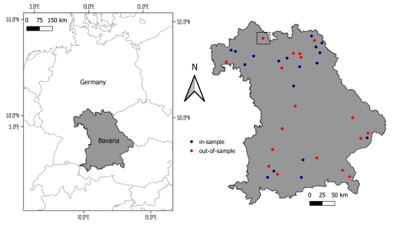
Figure 1: Study sites of the camera trap images used in this work. Two stations (black square) have almost the same location, the respective camera had to be moved during the study.

Table 1: Number of images per class.

Species	in-sample	out-of-sample	total
european hare	485	255	740
red deer	26	135	161
red fox	708	106	814
red squirrel	297	13	310
roe deer	6,074	7,010	13,084
wild boar	210	904	1,114
others	941	1,051	1,992
empty	15,627	14,274	29,901
total	24,368	23,748	48,116

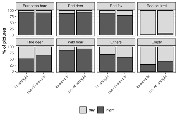
Figure 2: Distribution of day and night images per class for in-sample and out-of-sample images.

2.2 Pipeline for tuning and model training

We consider a data set $\mathcal{D}=\left(\left(\mathbf{x}^{(1)},y^{(1)}\right),\ldots,\left(\mathbf{x}^{(n)},y^{(n)}\right)\right)$ of labeled images, where $y^{(i)}\in\{1,\ldots,g\}$ is the label of image $\mathbf{x}^{(i)}$ and $g$ is the number of classes. The goal is to train a classification pipeline $\hat{\pi}(\cdot)$ that maps images $\mathbf{x}$ to probability scores $\hat{\pi}(\mathbf{x})$ of predicted hard labels $\hat{y}=\operatorname{arg\,max}_{k\in\{1,\ldots,g\}}\hat{\pi}_{k}(\mathbf{x})$. Our pipeline consists of two major parts: In the first part, bounding boxes of animals in the images are detected via object detection. In the second part, bounding-box images are classified with respect to animal species.

2.2.1 Classification pipeline with object detection and image classification

Object detection – from image level to bounding-box level

Often, a considerable fraction of each image does not show an animal (see Fig. 5 for some examples). If the entire image is passed to an image classifier, the classifier needs to cope with the challenge of detecting the important pixels and focusing on those. Predictive performance can be increased by providing bounding boxes of animals. Different object detection pipelines have been proposed in the literature; we use the Megadetector (MD) pipeline [Beery et al., 2019] for its high usability and good performance in prior studies [see Vélez et al., 2023, for a comparison]. MD produces (among other results which we do not use in the following) for every image $\mathbf{x}^{(i)}$ a (possibly empty) set of $m$ bounding-box coordinates with corresponding confidence values $\bm{c}^{(i)}=(c^{(i)}_{1},\dots,c^{(i)}_{m})\in[0,1]^{m}$ of capturing an animal. All bounding boxes with confidence $c^{(i)}_{j}\geq\alpha$ (high-conf BB) are passed on to the next step – the image classifier on the bounding-box level. All images that have no bounding boxes or only bounding boxes with a low confidence $c^{(i)}_{j}<\alpha$ (other BB) are considered empty. The confidence threshold $\alpha$ is either set to a fixed value beforehand or can be chosen in a data-driven manner and specifically tailored for the data set at hand. We opt for the latter approach and consider the threshold $\alpha$ to be a hyperparameter optimized during tuning.

Image classification at the level of bounding boxes

We consider the following preprocessing on the level of bounding-box images (bb-images).

(1) Cropping and resizing: For all bounding boxes with a confidence threshold of at least $\alpha$, we crop the respective part from the original image and resize it, such that we obtain $s$ square bb-images $\bm{z}^{(i)},i\in\{1,\dots,s\}$ of $224\times 224$ pixels, which is the optimal input size for networks pre-trained on ImageNet [Deng et al., 2009]. We assign each bb-image the label of the original image that it is part of; this only makes sense if images are pure in the sense that if an image shows animals, it only shows animals of a unique species. In our data, we did not encounter any image with mixed animal species, but this assumption needs to be asserted critically for other data sets – demanding to label on bounding-box level if the purity assumption does not hold.

(2) Augmentation: We augment the bb-images of the training data by optional rotation, flipping, and changing the contrast, and use up to three randomly sampled augmentations per image for the analyses in this paper .

(3) Transfer learning: As a last preprocessing step, we carry out a forward pass through a pre-trained image classification network, choosing between the available architectures, where we exclude the final fully-connected layers. The resulting data representation, whose structure the network has learned from millions of pre-training samples, encapsulates latent image properties from which classes can be predicted quite easily.

With the thus preprocessed data, we train an image classification model.

Predicting new images with the pipeline

Consider a set $\mathcal{D}_{new}=(\mathbf{x}^{(1)},\dots,\mathbf{x}^{(w)})$ of new images: First, we apply object detection, cropping and resizing, and the forward pass through the pre-trained model. The resulting data is used to predict the class scores of the bb-images $\mathcal{D}_{z,new}$ with the image classifier $\hat{\pi}(\mathbf{x})$. Then, the results of object detection and image classification are merged: The predicted label is set to “empty” for all images which (i) have no bounding boxes with a confidence of at least $\alpha$ or (ii) have bounding boxes that pass the threshold but are classified as “empty” by the image classifier. For all other images, the predicted label is set to the non-empty class with the highest weighted average of the bounding box predictions, where the MD confidences are used as weights. This weighted average is retained as final confidence about the class. This yields

1. predicted labels $\hat{y}^{(i)}$ for each image $\mathbf{x}^{(i)}\in\mathcal{D}_{new}$,

2. average weighted predicted class scores $\hat{\pi}_{k}^{(i)}$ for each class $k\in\{1,\ldots,g\}$ per image,

3. the total predicted number $o_{k}^{(i)}$ of each animal class per image, and

4. a final confidence score $d^{(i)}=\max_{k\in\{1,\ldots,g\}}\hat{\pi}_{k}^{(i)}$ per image, reflecting the highest class-wise score.

Optionally, images whose highest confidence for any class does not exceed a user-specified threshold, i.e., $d^{(i)}\leq\beta,$ may still remain “unlabeled”, thus giving the user the opportunity to label it manually in a later iteration of the AL process.

2.2.2 Tuning pipeline

Resampling strategy

The above pipeline comprises hyperparameters ( (i) megadetector threshold (ii) choice of the pre-trained network ) which cannot be learned during training but need to be optimized via hyperparameter tuning. Fig. 3 visualizes the resampling strategy and pipeline for tuning and evaluation: We divide $\mathcal{D}$ randomly (stratified by camera station) into data for tuning and training ($\mathcal{D}_{tune}$) and data for evaluating the model performance ($\mathcal{D}_{test}$), where $15\%$ are used for $\mathcal{D}_{test}$. Tuning data $\mathcal{D}_{tune}$ is further split into training data $\mathcal{D}_{train}$ and validation data $\mathcal{D}_{val}$, such that those sets comprise $70\%$ and $15\%$ of $\mathcal{D}$, respectively. Training data $\mathcal{D}_{train}$ is then used to train a classification model on the level of bounding boxes for each combination of hyperparameters; the best hyperparameter combination is chosen with respect to the performance of the pipeline on validation data $\mathcal{D}_{val}$. Finally, generalization errors of the classifier and the pipeline, endowed with the chosen hyperparameters, are estimated on the untouched test data $\mathcal{D}_{test}$.

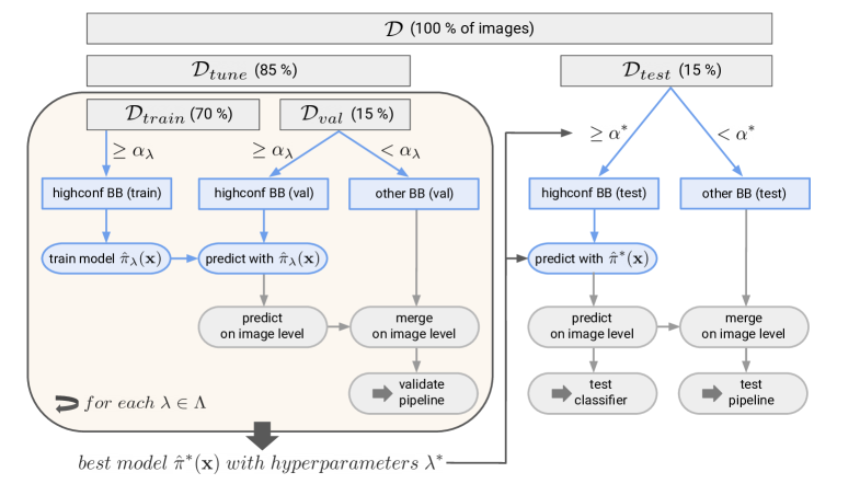
Figure 3: Resampling scheme. Hyperparameter tuning is carried out on tuning data $\mathcal{D}_{tune}$. Generalization errors using the best hyperparameters are estimated on untouched test data $\mathcal{D}_{test}$.

Tuning

We train a model $\hat{\pi}_{\bm{\lambda}}(\cdot)$ for each hyperparameter combination $\bm{\lambda}\in\bm{\Lambda}$ – where $\bm{\Lambda}$ is the corresponding search space – on $\mathcal{D}_{z,train}$ and evaluate the pipeline of object detection and image classification with this model $\hat{\pi}_{\bm{\lambda}}(\cdot)$ on $\mathcal{D}_{val}$.

Predicted labels are computed by combining the results of object detection and image classification – as explained above for new images. Evaluation metrics $\rho_{\bm{\lambda}}$ are computed for each hyperparameter combination separately. For our tuning process, one of the four alternatives recall, precision, F1-score, or accuracy can be chosen by the user – for the results presented in this paper, we choose the weighted F1-score. The hyperparameter combination yielding the highest $\rho_{\bm{\lambda}}$ on $\mathcal{D}_{val}$, i.e., $\bm{\lambda}^{*}=\operatorname{arg\,max}_{\bm{\lambda}\in\bm{\Lambda}}\rho_{\bm{\lambda}}$, is considered the best hyperparameter combination, the corresponding model is $\pi^{*}(\cdot)$.

Evaluation at the level of bounding boxes

We first carry out the object detection and the above preprocessing steps of cropping, resizing, and the forward-pass through the pre-trained model – as indicated by the respective value in $\bm{\lambda}^{*}$ – on $\mathcal{D}_{test}$. The labels of the resulting bb-images are predicted by $\pi^{*}(\mathbf{x})$ and an evaluation metric can be computed for the high-conf bb-images in $\mathcal{D}_{z,test}$.

Evaluation at the level of original images

As above, we merge the results of object detection and image classification for the images in $\mathcal{D}_{test}$ and compute the respective evaluation metric.

2.3 Pipeline for active learning

We propose the following active learning (AL) pipeline (see also Algorithm 1).

(1) Initialization: A data set of unlabeled images is provided by the user. If for some images, labels are already available, these can be used and hence no random sampling is necessary in step (2a). However, since the selection of images that are labeled might not be representative of the entire data set in practice, e.g., because all labels are from a very small and hence similar period of time, we generally recommend random sampling in the first iteration. If available, information about which images belong to the same camera station should be provided, too, to allow for stratification in the resampling process.

(2) AL loop: As long as the user is unsatisfied with the prediction performance of the current model (as reported by the evaluation step – and optionally by visual inspection), the active learning loop is carried out:

(2a) Image selection: A user-specified number of unlabeled images is selected by the AL engine. These are the images that have the highest value of a so-called “acquisition function”; the value of this function reflects the potential of an image for improving the model – we use softmax entropy. Optionally, this can be done stratified by camera stations. In the first iteration of the AL loop, where no model is available, image selection is done randomly.

(2b) Manual labeling: The selected images are labeled by a human expert.

(2c) Model training: A full step of tuning, training, and evaluation as described above is carried out, based on the available labeled data. If the time budget is limited, the user may consider skipping tuning here.

(3) Predict remaining unlabeled images: As the last step of the pipeline, all remaining unlabeled images are predicted by the final model.

For the evaluation of the trained models, a sufficiently large subset of the labeled images needs to be set apart as a test set. This test set is used only for evaluating the performance of the model and remains unchanged during the AL loop.

Algorithm 1 Active Learning Workflow (H: Human – M: Machine)

H: Load data (unlabeled or partly labeled) $\triangleright$ (1)

if No labeled images then

     M: Select random images to be labeled $\triangleright$ (2a)

     H: Label images manually $\triangleright$ (2b)

end if

M: Tune, train, evaluate initial model $\triangleright$ (2c)

while H: Not satisfied with test performance do $\triangleright$ (2)

     M: Select best images to be labeled via acquisition function $\triangleright$ (2a)

     H: Label images manually $\triangleright$ (2b)

     M: Tune, train, evaluate $\triangleright$ (2c)

end while

M: Predict all remaining unlabeled images with the last model $\triangleright$ (3)

3 Results

In the following, we show results for the Bavarian data presented in Section 2.1, Appendix A applies our method to a different dataset, obtained from the LILA database.

3.1 In-sample results

For tuning, training, and evaluating the models, we use a $70\%$-$15\%$-$15\%$ train-val-test split and report evaluation metrics only for the test set which is not seen during training or tuning of the models. As data, we use the 24,368 “in-sample” images shown in Table 1. As tuning search space $\bm{\Lambda}$ we use a grid consisting of all combinations of architecture $\in$ {InceptionResNetV2, Xception, DenseNet121}, which are all state-of-the-art across many image classification tasks and parameter-efficient at the same time, and MD threshold $\alpha\in\{0.1,0.3,0.5,0.7,0.9\}$. When writing this manuscript, the current version of MegaDetector is MDv5, which we use for our analyses (from the two versions MDv5a and MDv5b, we choose the former which is trained on more data). However, we also compare tuning results using the prior version MDv4 for two reasons: (a) Some of the seminal papers in wildlife camera trap image classification such as Norouzzadeh et al. [2021] use MDv4 with $\alpha=0.9$ without tuning and we want to make a sensible comparison here, and (b) the optimal confidence threshold may have changed in comparison to older versions, which we want to investigate for a fixed dataset, ruling out differences in the images analyzed as a reason for differing results. All reported numbers represent the average over results from three independent runs.

3.1.1 Benefit of tuning hyperparameters

Table 2 shows the weighted F1-score on $\mathcal{D}_{val}$ for the 8-class classification for different choices of the hyperparameters using MDv5. As can be seen, tuning the hyperparameters properly has a substantial impact on the predictive performance of the model. The bold first row reflects the optimal choice of hyperparameters which is used for the following experiments. Table 3 shows results for MDv4. We observe two key insights: (a) our pipeline with MDv5 is performing substantially better than with MDv4, and (b) the optimal hyperparameter configuration is differing very much. The second point underlines the importance of tuning the hyperparameters since there is no guarantee that for (a) other datasets or (b) other (versions of) object detectors the optimal hyperparameters are the same. Interestingly, the performance is more variable for MDv5 than for MDv4, meaning that proper tuning has more impact for the newer version.

Table 2: Hyperparameter tuning: best and worst configurations sorted by F1-score (MDv5)

Confidence	Architecture	F1-score
0.1	Xception	0.933
0.3	Xception	0.932
0.5	Xception	0.921
0.7	Xception	0.900
$\vdots$	$\vdots$	$\vdots$
0.9	Xception	0.781
0.9	DenseNet121	0.780
0.9	InceptionResNetV2	0.777

Table 3: Hyperparameter tuning: best and worst configurations sorted by F1-score (MDv4)

Confidence	Architecture	F1-score
0.5	Xception	0.909
0.7	Xception	0.908
0.9	InceptionResNetV2	0.908
$\vdots$	$\vdots$	$\vdots$
0.3	DenseNet121	0.899
0.1	InceptionResNetV2	0.894
0.1	DenseNet121	0.888

3.1.2 Empty vs. non-empty images

During tuning, the best confidence threshold was $\alpha=0.1$ for MDv5 and $\alpha=0.5$ for MDv4, respectively. We can now compare results for the binary classification of “empty” vs. “non-empty” for different choices of $\alpha$ in Table LABEL:tab:empty_resultsmdv5 for MDv5 and Table LABEL:tab:empty_resultsmdv4 for MDv4. The empty recall increases with $\alpha$ due to the fact that the MD is considering more images as empty. On the other hand, the non-empty recall decreases with $\alpha$, meaning that more non-empty images (i.e., animals) are retrieved for smaller $\alpha$. In fact, with tuned $\alpha=0.5$ for MDv4, the false-empty rate is $14.2\%$ less than with $\alpha=0.9$ (a common choice, e.g., Norouzzadeh et al. [2021]) ($10.9\%$ vs. $12.7\%$), meaning that $14.2\%$ fewer animal images are overlooked. From a practical perspective, this is highly desirable: While it is no big effort to manually discard some images that are empty but labeled as non-empty, it is not feasible to detect non-empty images that are labeled as empty without screening all the images again – which is exactly what we wish to avoid by using an automatic image classifier. This shows that tuning $\alpha$ is also beneficial for the “empty” vs. “non-empty” performance and increases the number of detected animals overall.

Table 4: Empty vs. non-empty images (MDv5), “no MD” shows metrics for not using object detection at all, hence only image classification on entire images.

			empty			non-empty
Confidence	Accuracy	Precision	Recall	F1	Precision	Recall	F1
no MD	0.920	0.913	0.969	0.940	0.936	0.830	0.880
0.1	0.962	0.950	0.993	0.971	0.986	0.906	0.944
0.3	0.959	0.946	0.994	0.969	0.987	0.899	0.941
0.5	0.947	0.927	0.996	0.960	0.991	0.861	0.922
0.7	0.927	0.898	0.998	0.946	0.996	0.799	0.887
0.9	0.816	0.777	0.999	0.874	0.997	0.491	0.658

Table 5: Empty vs. non-empty images (MDv4).

			empty			non-empty
Confidence	Accuracy	Precision	Recall	F1	Precision	Recall	F1
0.1	0.949	0.950	0.973	0.961	0.948	0.907	0.927
0.3	0.952	0.947	0.981	0.964	0.963	0.900	0.930
0.5	0.949	0.943	0.982	0.962	0.964	0.891	0.926
0.7	0.952	0.940	0.990	0.964	0.979	0.885	0.930
0.9	0.950	0.934	0.991	0.962	0.981	0.873	0.924

3.1.3 Multi-class model performance

From here on, we are focusing on the results of MDv5. Table LABEL:tab:ins-oos, first and second row, lists overall metrics of the classification performance on $\mathcal{D}_{test}$. The first row contains results of omitting object detection and directly performing image classification on the entire images; a comparison with the second row reveals a clear benefit of using the pipeline of object detection and image classification. Fig. 4 shows the detailed predictive performance of the tuned pipeline. Performance for larger classes (in terms of the number of images, not of animal size) such as “roe deer” is better than for smaller classes such as “wild boar”. The class “other” proves difficult to detect, which might be due to the fact that this class is rather heterogeneous as it consists of (i) other animal species than considered here (hence low numbers per class) and (ii) images where the true animal class could not be determined by the human annotators with sufficient confidence.

Table 6: Multi-class classification (MDv5). Precision and F1-score are weighted averages of 8 classes, (weighted recall is not shown since equal to accuracy by definition).

	Accuracy	Precision	F1
no MD (in-sample)	0.865	0.869	0.856
In-sample	0.933	0.929	0.930
Out-of-sample	0.868	0.874	0.867
Active learning – 37$\%$	0.926	0.921	0.919
Active learning – 100$\%$	0.932	0.929	0.927

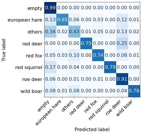
Figure 4: In-sample performance

Fig. 5 displays some misclassified images and points to cases where the classification is wrong. Reasons seem to be, among others: Extreme close-up (5(a)), difficulties due to partial occlusion (5(b)), poor lighting – and hence no bounding box by MD (5(c)), very small objects (5(d)), wrong bounding box by MD (5(e)), and wrong human label (5(f)). In the last case, the prediction counts as misclassified since the human label and the predicted label do not match, but note that actually both the prediction and the human label are wrong in this case, since this is a red deer, not a roe deer.

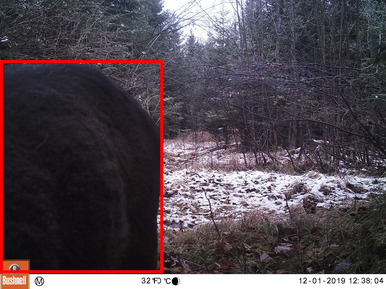
(a) Extreme close-up. Label: roe deer, predicted: others, confidence: 0.74

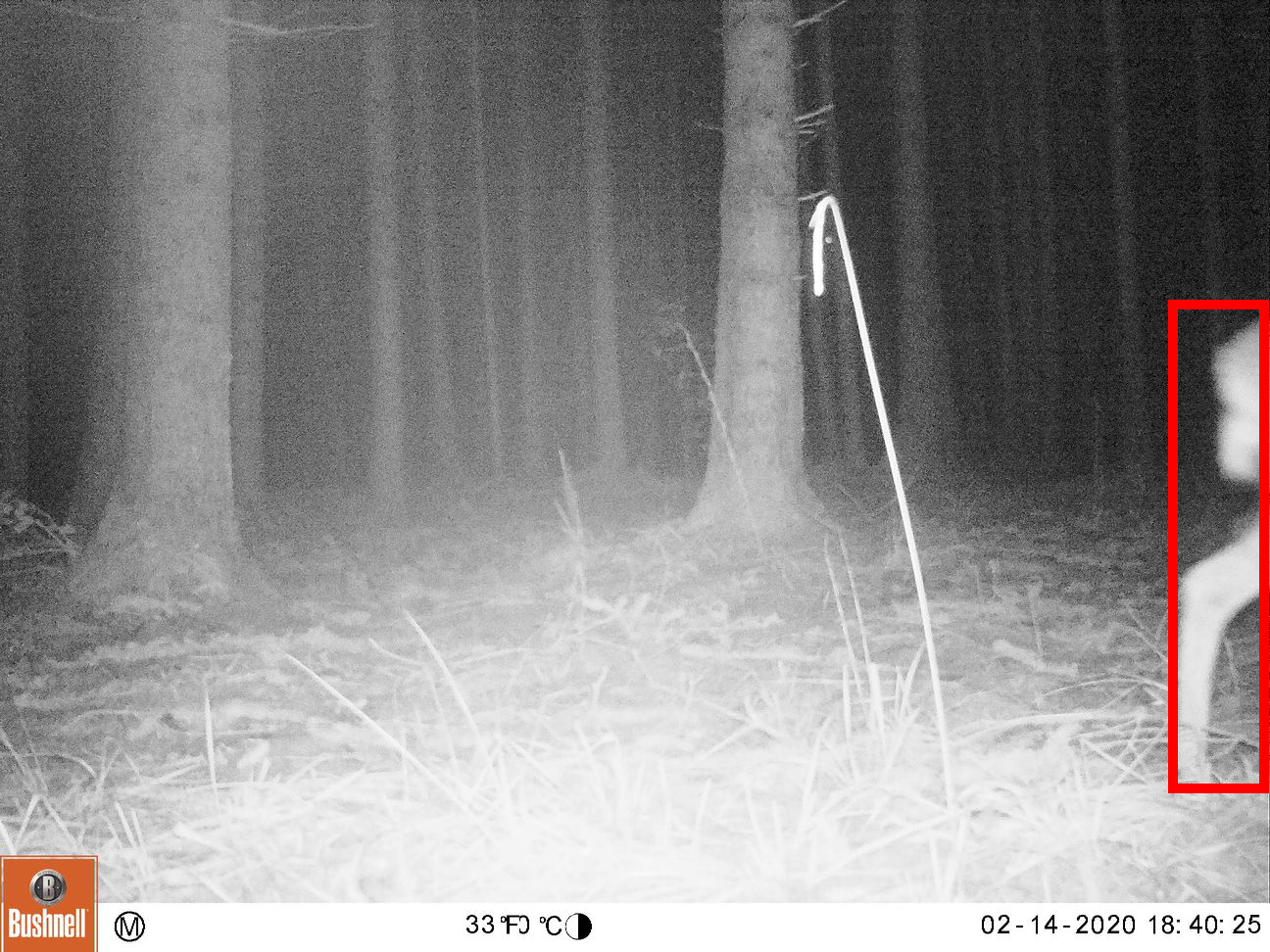
(b) Partial occlusion. Label: roe deer, predicted: others, confidence: 0.67

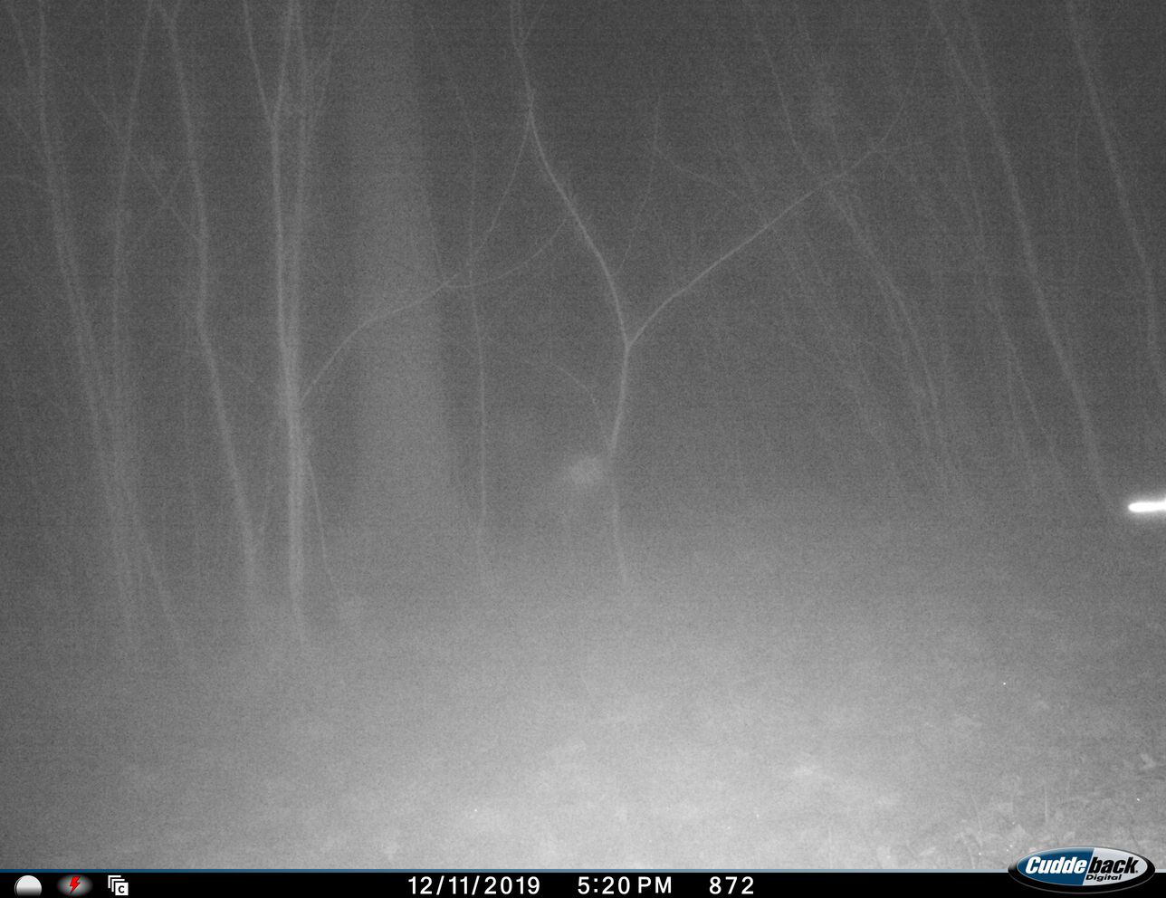
(c) Poor light. Label: roe deer, predicted: empty, confidence: 1.00

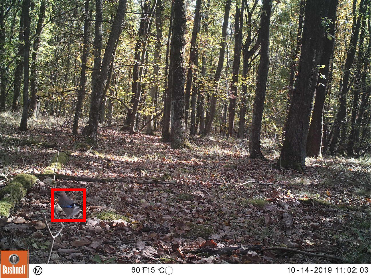
(d) Small objects. Label: others, predicted: red squirrel, confidence: 0.43

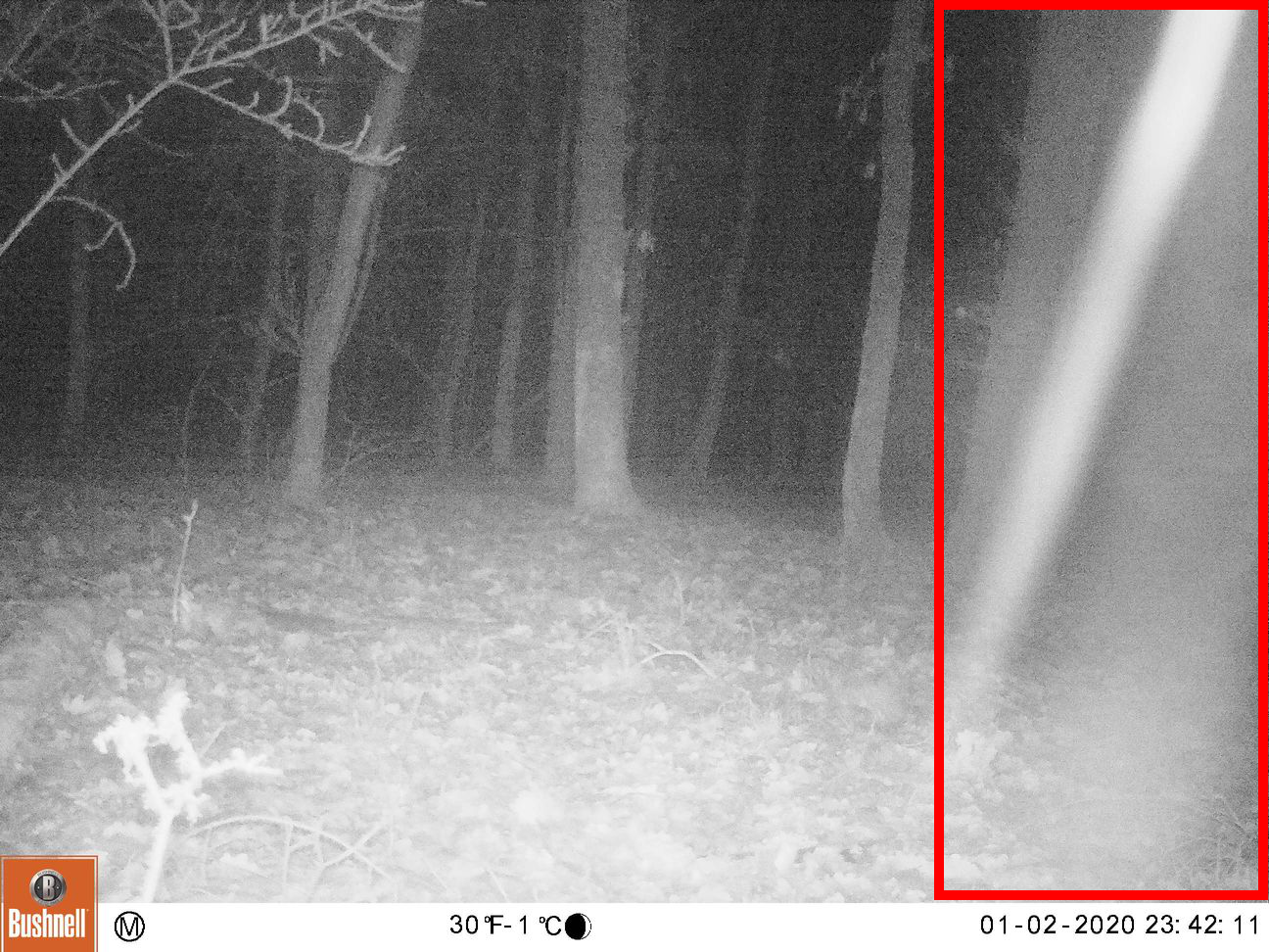
(e) Wrong bounding box. Label: empty, predicted: roe deer, confidence: 0.65

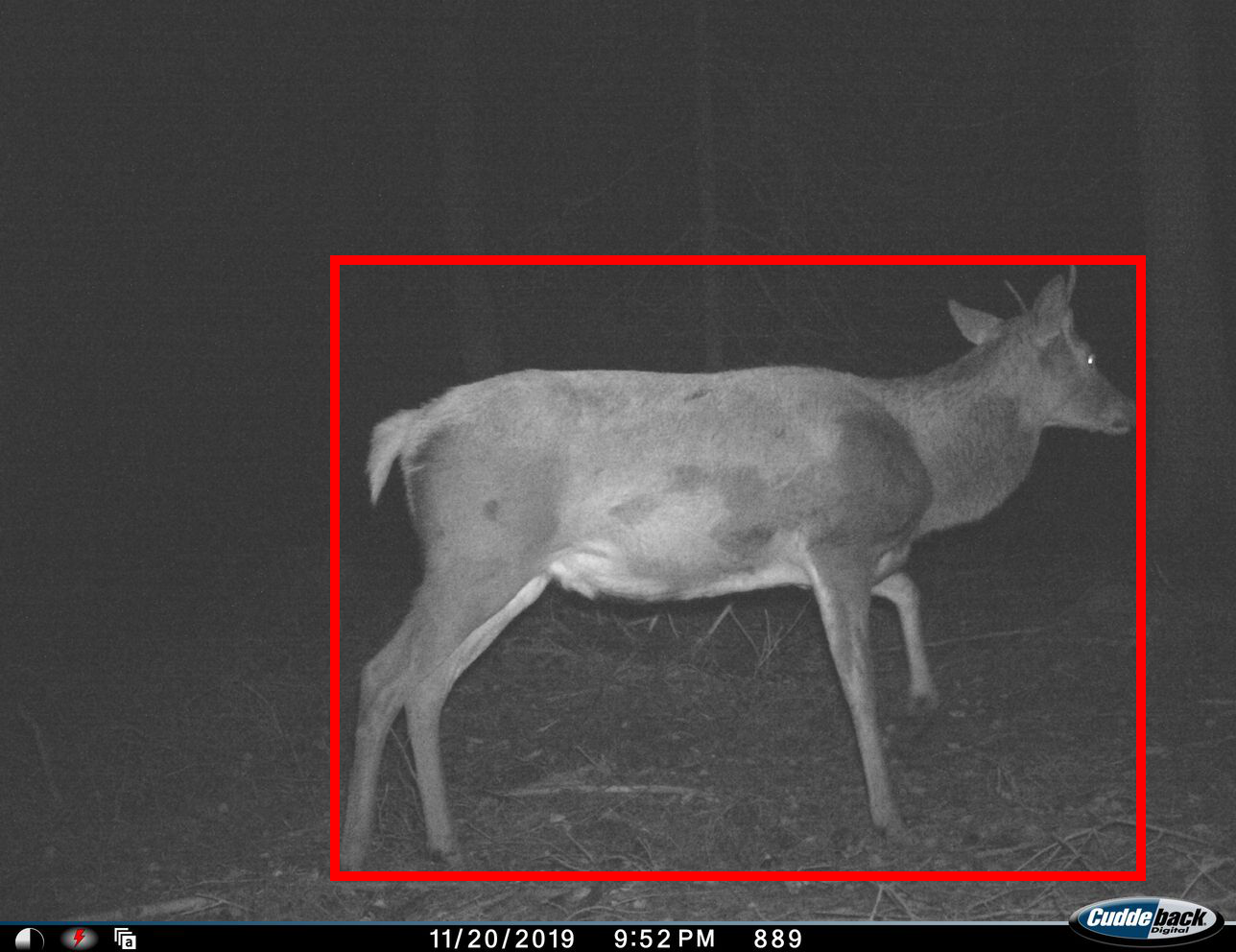
(f) Wrong human label. Label: others, predicted: roe deer, confidence: 0.65

Figure 5: Misclassified images

3.2 Out-of-sample results

For a sensible comparison of OOS results, i.e., comparing model performance without AL and with AL – and also different stages of AL–, we sampled a random test set from the OOS images, consisting of 15% of the images, stratified by camera station. This test set comprises 3,667 images, from which 1,503 images were identified as non-empty by the MD at confidence $\alpha=0.1$, is never used for training or tuning, and remains unchanged over all model comparisons.

3.2.1 Model performance out-of-sample without active learning

Table LABEL:tab:ins-oos, third row, shows the predictive performance of predicting the OOS test data with the model trained on the entire in-sample data; the drop in predictive performance is expected and in line with results in the literature. Fig. 6 shows detailed results of the image classifier for the OOS test data. A comparison with the class distribution between in-sample and out-of-sample data reveals that performance is especially low where the distribution has shifted most. For example, there are only 26 red deers in the entire training data; it is hence unsurprising that the predictive performance for this class will be rather low. This distribution shift between train and test data is exactly the problem of OOS prediction which shall be remedied by using active learning: By adding more and more training data from the new distribution, the performance should increase until a satisfying level is reached.

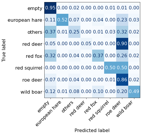
Figure 6: Out-of-sample performance without AL.

3.2.2 Model performance out-of-sample with active learning

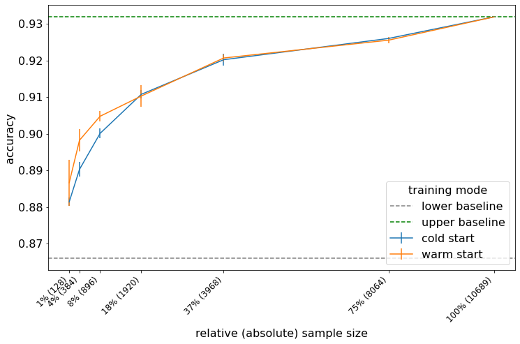
Figure 7: Active-learning performance (8-class accuracy) for cold and warm start as compared to out-of-sample prediction (lower horizontal line) and training on the entire data set (upper horizontal line). Error bars indicate variability over 3 different random seeds.

Fig. 7 shows the results of the active learning pipeline. For a proper assessment of the benefit of active learning, we compare it with two baselines: The lower baseline is the model trained on the in-sample data (Table LABEL:tab:ins-oos, third row). The upper baseline is a model trained on the entire OOS data (Table LABEL:tab:ins-oos, last row). We compare two active learning strategies; for both strategies, we use the architecture that was found to be optimal in the above tuning procedure, i.e., the Xception architecture. The classification head (i.e., the set of final linear layers) is replaced by a new classification head with freshly initialized weights. Note that this enables tailoring the pipeline to tasks with an arbitrary set of classes by simply adjusting the number of output units in the last layer (in contrast to directly using the model trained on the in-sample data which is consequently restricted to the classes seen during training). The two strategies differ in the following:

• Cold-start: For the rest of the neural net (the so-called backbone responsible for the task of learning a suitable data representation), the weights pre-trained on ImageNet are used.

• Warm-start: For the backbone, the weights pre-trained on ImageNet and on the in-sample data are used.

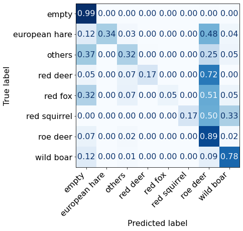
Figure 8: Out-of-sample performance with AL using $37\%$ of available data, i.e., 3,968 images.

As can be seen in the very left part of Fig. 7, both active learning strategies outperform the lower baseline (which has never encountered samples from the OOS data) already in the initial iterations. This is somewhat surprising since in the first iteration only 128 images are used for training – where the lower baseline is trained on the entire in-sample data of 24,368 images – and underlines the importance of tailoring the model to the specific dataset at hand. With an increasing amount of images, the active learning models improve further. In the first iterations, warm-starting has a substantial advantage over cold-starting, this effect vanishes after using 1920 images for training. This means that the information in the OOS data is eventually better than the information in the in-sample data. Using a relative sample size of $37\%$, i.e. 3,968 images, we already reach $99.4\%$ of the performance of the upper baseline, showing the benefit of using active learning.

Note the general applicability of the active learning approaches: Since we replace the classification head, the strategy can be used to learn models predicting any set of classes. This allows learning well-performing models with just a small number of manually annotated images. A further advantage is that the number of images to be labeled by a human does not have to be fixed beforehand: The active learning procedure can be carried out iteratively until a satisfying performance is reached, thus using the human annotation labor very efficiently. Furthermore, if the new images are expected to be rather similar to the existing ones (e.g., by setting up a new camera station in a territory comprising the same fauna), warm-starting may be beneficial and can decrease the number of images needed even more.

4 Discussion and Conclusions

We presented two methodological advances in using deep learning methods for wildlife image classification. First, a thorough tuning procedure for optimizing the hyperparameters of a multi-step pipeline, consisting of object detection and image classification. Second, an active learning component that enables efficient training of a high-performing model on new data, potentially from a new monitoring location or involving previously unseen animal species. We accompany the methodological developments with ready-to-use software which does not require programming skills of the user. Thereby, we leverage the potential of deep learning and active learning for a broad target group including all researchers in ecology, even with different analytical backgrounds.

Our results showed that tuning the hyperparameters has indeed an effect on the predictive performance of the resulting models. While taking well-performing hyperparameter choices from the literature might be a solid start in a project, tuning increases performance. The need for thorough tuning is even higher if no such hyperparameters choices from the literature exist, e.g., for new versions of an object detector like MegaDetector. The overall performance of our models is not competitive with some contributions in the literature which is due to the fact that we aim at smaller projects and consider a data set of around 50,000 images, while others use several millions of images. However, we show that the active learning component quickly helps improve the results for out-of-sample images and that warm-starting additionally increases performance in the first iterations. Note that while we carefully designed in-sample and out-of-sample data sets making sure that no image of the out-of-sample set stems from a camera station contained in the in-sample set, these images are still from comparable regions in Bavaria, Germany. Transferring this to other regions of the world and hence to backgrounds that might be deviating more from the Bavarian images, will reduce the initial (warm-start) performance, making it even more important to train the model actively with images from those new camera stations.

While the methods are indeed easy to use, it is helpful to have access to sufficient computing resources. Although it is possible to use the methods on a local machine with only CPUs, working on a machine with a GPU is substantially faster. A rather time-consuming step is the application of the Megadetector for finding the bounding boxes, which, however, needs to be carried out only once before starting the active learning loop. There are attempts to approximate the Megadetector with a far smaller object detection method [e.g., Rigoudy et al., 2022] saving computing time. We still opt for the Megadetector due to its very convincing performance. The other time-consuming step is the repeated tuning of the hyperparameters which can slow down the progress in the active learning loop; we, therefore, allow to optionally skip the tuning inside the active learning. In many applications, though, human labor will remain the scarcest resource, and the need for it is greatly alleviated with our pipeline.

Future work

There are some directions of future work that we would like to pursue: 1. Labeling bounding boxes instead of original images could further improve the performance of the models. 2. More complex acquisition functions in the active learning pipeline could improve efficiency. 3. We already have first results on incorporating methods from explainable AI in the pipeline. Explaining the predictions of the model can help to find systematic errors. 4. Quantifying the predictive uncertainty of the model and the derived population count might give more realistic insights into the data. 5. Using metadata such as time, date, etc. as additional input has the potential to further improve the results. 6. Combining machine learning and domain knowledge could be a promising next step, see, e.g., Tuia et al. [2022]. 7. Finally, we plan on developing an R package that helps researchers with downstream analyses of the information from the image classification pipeline.

Funding

CB, WP, and AM received funding within the project LandKlif, funded by the Bavarian State Ministry of Science and the Arts in the context of the Bavarian Climate Research Network (bayklif). HE, WP, and CB received funding from the Bavarian State Ministry of Agriculture and Forestry (grant number ST375). TW received funding from the Deutsche Forschungsgemeinschaft (DFG, German Research Foundation) as part of BERD@NFDI (grant number 460037581). LW received funding from the DAAD programme Konrad Zuse Schools of Excellence in Artificial Intelligence, sponsored by the Federal Ministry of Education and Research, Germany.

Conflict of Interest statement

The authors declare no conflicts of interest.

Author Contributions

Conceptualization, LB, HE, WP, CB, and AM; Methodology, LB, OC, LW, and TW; Software, LB, OC, LW, and TW; Formal analysis, LB, OC, and LW; Resources, WP and AM; Data curation, CB, HE and HN; Writing - Original Draft, LB; Writing - Review & Editing, all authors; Visualization, OC and LW

Data Availability

The image data set will be archived on Dryad upon acceptance.

Appendix A Additional results on different data

To investigate the behavior of our proposed method on data from a different study site, we analyzed images from the Channel Islands Camera Traps [The Nature Conservancy, 2021] obtained via the LILA database. We used a subset of 50,868 images (from 7 out of 73 camera stations) to make the size comparable to the Bavarian data analyzed above and also split the images into in-sample and out-of-sample data by camera station (3 and 4 stations for in-sample and out-of-sample, respectively). The dataset comprises 4 animal classes as well as an “empty” and an “other” class, where we removed the latter because it contains just a minimal amount of images (less than $0.14\%$). Table 7 summarizes the distribution of classes in the images used here.

Table 7: Number of images per class (Channel Islands).

Species	in-sample	out-of-sample	total
fox	4,147	12,462	16,609
skunk	37	142	179
rodent	1,397	483	1,880
bird	210	568	778
empty	14,445	16,977	31,422
total	20,236	30,632	50,868

We applied the same tuning strategy as explained above in Section 3.1 and show the results in Table 8. The best hyperparameter combination is again Xception with a confidence threshold of $\alpha=0.1$ and as above, high thresholds of $\alpha=0.9$ perform worst. We can also see that the model is performing better than for the data from Bavaria, see Figure 9 for detailed results on the test data (in-sample). As before, performance for larger classes (fox, rodent) is higher than for classes with fewer images (skunk, bird).

Table 8: Hyperparameter tuning: best and worst configurations sorted by F1-score (MDv5, Channel Islands)

Confidence	Architecture	F1-score
0.1	Xception	0.974
0.3	Xception	0.973
0.1	InceptionResNetV2	0.965
0.5	Xception	0.964
$\vdots$	$\vdots$	$\vdots$
0.9	InceptionResNetV2	0.814
0.9	DenseNet121	0.814
0.9	Xception	0.813

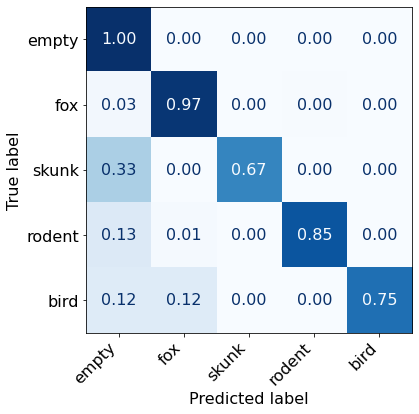
Figure 9: In-sample performance (Channel Islands)

Table LABEL:tab:empty_resultsmdv5_channel shows the performance of the pipeline in the binary classification of empty vs. non-empty for different thresholds and using Xception, also underlining the stronger performance for smaller thresholds.

Table 9: Empty vs. non-empty images (MDv5, Channel Islands)

			empty			non-empty
Confidence	Accuracy	Precision	Recall	F1	Precision	Recall	F1
0.1	0.982	0.980	0.995	0.988	0.987	0.949	0.968
0.3	0.981	0.978	0.995	0.987	0.988	0.943	0.965
0.5	0.974	0.966	0.999	0.982	0.997	0.911	0.952
0.7	0.937	0.919	1.000	0.958	1.000	0.778	0.875
0.9	0.862	0.839	1.000	0.912	1.000	0.514	0.679

Table LABEL:tab:ins-oos_channel compares the performance on in-sample (first row) and out-of-sample (second row), showing only a minimal drop in performance when moving from in-sample to out-of-sample (see also Figure 10 for detailed out-of-sample results on the test set). The active learning pipeline again improves the results (third row) and achieves 99.6% of the performance compared to using the entire out-of-sample training data (fourth row) by just training on 3,968 images, i.e., 29% of the images. The higher performance of AL-100$\%$ compared to in-sample suggests that the out-of-sample data poses an easier challenge for the specific case of the Channel Islands data. The largest class (fox) has fewer “false-empty” predictions in out-of-sample (Figure 10) compared to in-sample (Figure 9) and the overall drop in performance (Table LABEL:tab:ins-oos_channel, first and second row) stems from the smaller classes. Using AL, the performance on these smaller classes increases (Figure 12).

Table 10: Multi-class classification (MDv5, Channel Islands). Precision and F1-score are weighted averages of 5 classes.

	Accuracy	Precision	F1
In-sample	0.979	0.979	0.979
Out-of-sample	0.978	0.977	0.976
Active learning – 29%	0.983	0.983	0.983
Active learning – 100%	0.987	0.986	0.986

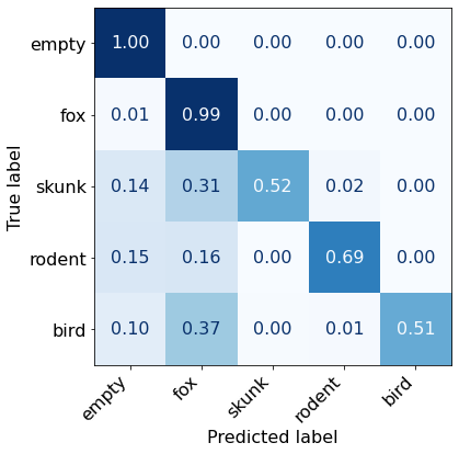
Figure 10: Out-of-sample performance without AL (Channel Islands).

Figure 11 shows how quickly the performance increases while iteratively including more labeled images for training in the active learning loop. We can see that accuracy surpasses the lower baseline and reaches a close-to-optimal level early on. Again, the algorithm achieves better performance overall on the Channel Islands data compared to the Bavarian data. In this case, warm-starting does not improve the performance substantially, compared to cold-starting. Finally, Figure 12 shows detailed classification results for active learning after using 3,968 images for training. While performance on the larger classes is high for out-of-sample as well, the active learning procedure benefits the smaller classes, identifying 25.0% more skunks, 15.9% more rodents, and 56.9% more birds correctly.

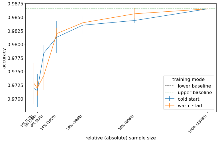
Figure 11: Active-learning performance (5-class accuracy, Channel Islands) for cold and warm start as compared to out-of-sample prediction (lower horizontal line) and training on the entire data set (upper horizontal line). Error bars indicate variability over 3 different random seeds.

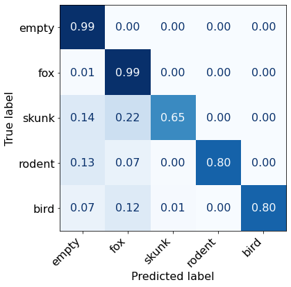
Figure 12: Out-of-sample performance with AL using $29\%$ of available data (Channel Islands).

References

- Abadi et al. [2015] M. Abadi, A. Agarwal, P. Barham, E. Brevdo, Z. Chen, C. Citro, G. S. Corrado, A. Davis, J. Dean, M. Devin, S. Ghemawat, I. Goodfellow, A. Harp, G. Irving, M. Isard, Y. Jia, R. Jozefowicz, L. Kaiser, M. Kudlur, J. Levenberg, D. Mané, R. Monga, S. Moore, D. Murray, C. Olah, M. Schuster, J. Shlens, B. Steiner, I. Sutskever, K. Talwar, P. Tucker, V. Vanhoucke, V. Vasudevan, F. Viégas, O. Vinyals, P. Warden, M. Wattenberg, M. Wicke, Y. Yu, and X. Zheng. TensorFlow: Large-Scale Machine Learning on Heterogeneous Systems, 2015. URL https://www.tensorflow.org/.
- Auer et al. [2021] D. Auer, P. Bodesheim, C. Fiderer, M. Heurich, and J. Denzler. Minimizing the Annotation Effort for Detecting Wildlife in Camera Trap Images with Active Learning. In INFORMATIK 2021, pages 547–564. Gesellschaft für Informatik, Bonn, 2021. doi: 10.18420/informatik2021-042.
- Beery et al. [2018] S. Beery, G. Van Horn, and P. Perona. Recognition in Terra Incognita. In V. Ferrari, M. Hebert, C. Sminchisescu, and Y. Weiss, editors, Computer Vision – ECCV 2018, Lecture Notes in Computer Science, pages 472–489, Cham, 2018. Springer International Publishing. doi: 10.1007/978-3-030-01270-0_28.
- Beery et al. [2019] S. Beery, D. Morris, and S. Yang. Efficient Pipeline for Camera Trap Image Review. arXiv, 2019. doi: 10.48550/arXiv.1907.06772.
- Bischl et al. [2023] B. Bischl, M. Binder, M. Lang, T. Pielok, J. Richter, S. Coors, J. Thomas, T. Ullmann, M. Becker, A.-L. Boulesteix, D. Deng, and M. Lindauer. Hyperparameter optimization: Foundations, algorithms, best practices, and open challenges. WIREs Data Mining and Knowledge Discovery, 2023. doi: 10.1002/widm.1484.
- Bolger et al. [2012] D. T. Bolger, T. A. Morrison, B. Vance, D. Lee, and H. Farid. A computer-assisted system for photographic mark–recapture analysis. Methods in Ecology and Evolution, 3(5):813–822, 2012. doi: 10.1111/j.2041-210X.2012.00212.x.
- Chen et al. [2014] G. Chen, T. X. Han, Z. He, R. Kays, and T. Forrester. Deep convolutional neural network based species recognition for wild animal monitoring. In 2014 IEEE International Conference on Image Processing (ICIP), pages 858–862, 2014. doi: 10.1109/ICIP.2014.7025172.
- Chollet [2017] F. Chollet. Xception: Deep Learning with Depthwise Separable Convolutions. In 2017 IEEE Conference on Computer Vision and Pattern Recognition (CVPR), pages 1800–1807, Honolulu, HI, 2017. IEEE. doi: 10.1109/CVPR.2017.195.
- Chollet et al. [2015] F. Chollet et al. Keras. https://keras.io, 2015.
- Christin et al. [2019] S. Christin, E. Hervet, and N. Lecomte. Applications for deep learning in ecology. Methods in Ecology and Evolution, 10(10):1632–1644, 2019. doi: 10.1111/2041-210X.13256.
- Curry et al. [2021] R. Curry, C. Trotter, and A. S. McGough. Application of deep learning to camera trap data for ecologists in planning / engineering – Can captivity imagery train a model which generalises to the wild? arXiv, 2021. doi: 10.48550/arXiv.2111.12805.
- Delisle et al. [2021] Z. J. Delisle, E. A. Flaherty, M. R. Nobbe, C. M. Wzientek, and R. K. Swihart. Next-Generation Camera Trapping: Systematic Review of Historic Trends Suggests Keys to Expanded Research Applications in Ecology and Conservation. Frontiers in Ecology and Evolution, 9, 2021.
- Deng et al. [2009] J. Deng, W. Dong, R. Socher, L.-J. Li, K. Li, and L. Fei-Fei. Imagenet: A large-scale hierarchical image database. In 2009 IEEE conference on computer vision and pattern recognition, pages 248–255, 2009. doi: 10.1109/CVPR.2009.5206848.
- Gimenez et al. [2021] O. Gimenez, M. Kervellec, J.-B. Fanjul, A. Chaine, L. Marescot, Y. Bollet, and C. Duchamp. Trade-off between deep learning for species identification and inference about predator-prey co-occurrence: Reproducible R workflow integrating models in computer vision and ecological statistics. arXiv, 2021. doi: 10.48550/arXiv.2108.11509.
- Gomez Villa et al. [2017] A. Gomez Villa, A. Salazar, and F. Vargas. Towards automatic wild animal monitoring: Identification of animal species in camera-trap images using very deep convolutional neural networks. Ecological Informatics, 41:24–32, 2017. doi: 10.1016/j.ecoinf.2017.07.004.
- Huang et al. [2017] G. Huang, Z. Liu, L. van der Maaten, and K. Q. Weinberger. Densely Connected Convolutional Networks. In Proceedings of the IEEE Conference on Computer Vision and Pattern Recognition (CVPR), 2017. doi: 10.1109/CVPR.2017.243.
- Hutter et al. [2019] F. Hutter, L. Kotthoff, and J. Vanschoren, editors. Automated Machine Learning - Methods, Systems, Challenges. Springer, 2019. doi: 10.1007/978-3-030-05318-5.
- Kellenberger et al. [2019] B. Kellenberger, D. Marcos, S. Lobry, and D. Tuia. Half a Percent of Labels is Enough: Efficient Animal Detection in UAV Imagery Using Deep CNNs and Active Learning. IEEE Transactions on Geoscience and Remote Sensing, 57(12):9524–9533, Dec. 2019. doi: 10.1109/TGRS.2019.2927393.
- Koh et al. [2021] P. W. Koh, S. Sagawa, H. Marklund, S. M. Xie, M. Zhang, A. Balsubramani, W. Hu, M. Yasunaga, R. L. Phillips, I. Gao, T. Lee, E. David, I. Stavness, W. Guo, B. Earnshaw, I. Haque, S. M. Beery, J. Leskovec, A. Kundaje, E. Pierson, S. Levine, C. Finn, and P. Liang. WILDS: A Benchmark of in-the-Wild Distribution Shifts. In Proceedings of the 38th International Conference on Machine Learning. PMLR, 2021.
- Miao et al. [2021] Z. Miao, Z. Liu, K. M. Gaynor, M. S. Palmer, S. X. Yu, and W. M. Getz. Iterative human and automated identification of wildlife images. Nature Machine Intelligence, 3(10):885–895, 2021. doi: 10.1038/s42256-021-00393-0.
- Moeller et al. [2018] A. K. Moeller, P. M. Lukacs, and J. S. Horne. Three novel methods to estimate abundance of unmarked animals using remote cameras. Ecosphere, 9(8):e02331, 2018. doi: 10.1002/ecs2.2331.
- Norouzzadeh et al. [2018] M. S. Norouzzadeh, A. Nguyen, M. Kosmala, A. Swanson, M. S. Palmer, C. Packer, and J. Clune. Automatically identifying, counting, and describing wild animals in camera-trap images with deep learning. Proceedings of the National Academy of Sciences, 115(25):E5716–E5725, 2018. doi: 10.1073/pnas.1719367115.
- Norouzzadeh et al. [2021] M. S. Norouzzadeh, D. Morris, S. Beery, N. Joshi, N. Jojic, and J. Clune. A deep active learning system for species identification and counting in camera trap images. Methods in Ecology and Evolution, 12(1):150–161, 2021. doi: 10.1111/2041-210X.13504.
- Ottoni et al. [2022] A. L. C. Ottoni, M. S. Novo, and D. B. Costa. Hyperparameter tuning of convolutional neural networks for building construction image classification. The Visual Computer, 2022. doi: 10.1007/s00371-021-02350-9.
- Redlich et al. [2022] S. Redlich, J. Zhang, C. Benjamin, M. S. Dhillon, J. Englmeier, J. Ewald, U. Fricke, C. Ganuza, M. Haensel, T. Hovestadt, J. Kollmann, T. Koellner, C. Kübert-Flock, H. Kunstmann, A. Menzel, C. Moning, W. Peters, R. Riebl, T. Rummler, S. Rojas-Botero, et al. Disentangling effects of climate and land use on biodiversity and ecosystem services—A multi-scale experimental design. Methods in Ecology and Evolution, 13(2):514–527, 2022. doi: 10.1111/2041-210X.13759.
- Rigoudy et al. [2022] N. Rigoudy, A. Benyoub, A. Besnard, C. Birck, Y. Bollet, Y. Bunz, N. D. Backer, G. Caussimont, A. Delestrade, L. Dispan, J.-F. Elder, J.-B. Fanjul, J. Fonderflick, M. Garel, W. Gaudry, A. Gérard, O. Gimenez, A. Hemery, A. Hemon, J.-M. Jullien, et al. The DeepFaune initiative: a collaborative effort towards the automatic identification of the French fauna in camera-trap images. bioRxiv, 2022. doi: 10.1101/2022.03.15.484324.
- Rowcliffe et al. [2008] J. M. Rowcliffe, J. Field, S. T. Turvey, and C. Carbone. Estimating animal density using camera traps without the need for individual recognition. Journal of Applied Ecology, 45(4):1228–1236, 2008. doi: 10.1111/j.1365-2664.2008.01473.x.
- Royle [2004] J. A. Royle. N-Mixture Models for Estimating Population Size from Spatially Replicated Counts. Biometrics, 60(1):108–115, 2004. doi: 10.1111/j.0006-341X.2004.00142.x.
- Schneider et al. [2019] S. Schneider, G. W. Taylor, S. Linquist, and S. C. Kremer. Past, present and future approaches using computer vision for animal re-identification from camera trap data. Methods in Ecology and Evolution, 10(4):461–470, 2019. doi: 10.1111/2041-210X.13133.
- Schneider et al. [2020] S. Schneider, S. Greenberg, G. W. Taylor, and S. C. Kremer. Three critical factors affecting automated image species recognition performance for camera traps. Ecology and Evolution, 10(7):3503–3517, 2020. doi: 10.1002/ece3.6147.
- Settles [2009] B. Settles. Active Learning Literature Survey. Computer Sciences Technical Report 1648, University of Wisconsin–Madison, 2009.
- Shepley et al. [2021] A. Shepley, G. Falzon, P. Meek, and P. Kwan. Automated location invariant animal detection in camera trap images using publicly available data sources. Ecology and Evolution, 11(9):4494–4506, 2021.
- Shorten and Khoshgoftaar [2019] C. Shorten and T. M. Khoshgoftaar. A survey on Image Data Augmentation for Deep Learning. Journal of Big Data, 6(1):60, 2019. doi: 10.1186/s40537-019-0197-0.
- Swanson et al. [2015] A. Swanson, M. Kosmala, C. Lintott, R. Simpson, A. Smith, and C. Packer. Data from: Snapshot Serengeti, high-frequency annotated camera trap images of 40 mammalian species in an African savanna. Dryad Digital Repository, 2015. doi: 10.5061/dryad.5pt92.
- Szegedy et al. [2016] C. Szegedy, S. Ioffe, V. Vanhoucke, and A. Alemi. Inception-v4, Inception-ResNet and the Impact of Residual Connections on Learning. arXiv, 2016. doi: 10.48550/arXiv.1602.07261.
- Tabak et al. [2019] M. A. Tabak, M. S. Norouzzadeh, D. W. Wolfson, S. J. Sweeney, K. C. Vercauteren, N. P. Snow, J. M. Halseth, P. A. Di Salvo, J. S. Lewis, M. D. White, B. Teton, J. C. Beasley, P. E. Schlichting, R. K. Boughton, B. Wight, E. S. Newkirk, J. S. Ivan, E. A. Odell, R. K. Brook, P. M. Lukacs, et al. Machine learning to classify animal species in camera trap images: Applications in ecology. Methods in Ecology and Evolution, 10(4):585–590, 2019. doi: 10.1111/2041-210X.13120.
- Tabak et al. [2020] M. A. Tabak, M. S. Norouzzadeh, D. W. Wolfson, E. J. Newton, R. K. Boughton, J. S. Ivan, E. A. Odell, E. S. Newkirk, R. Y. Conrey, J. Stenglein, F. Iannarilli, J. Erb, R. K. Brook, A. J. Davis, J. Lewis, D. P. Walsh, J. C. Beasley, K. C. VerCauteren, J. Clune, and R. S. Miller. Improving the accessibility and transferability of machine learning algorithms for identification of animals in camera trap images: MLWIC2. Ecology and Evolution, 10(19):10374–10383, 2020. doi: 10.1002/ece3.6692.
- Tabak et al. [2022] M. A. Tabak, D. Falbel, T. Hamzeh, R. K. Brook, J. A. Goolsby, L. D. Zoromski, R. K. Boughton, N. P. Snow, K. C. VerCauteren, and R. S. Miller. CameraTrapDetectoR: Automatically detect, classify, and count animals in camera trap images using artificial intelligence. bioRxiv, 2022. doi: 10.1101/2022.02.07.479461.
- Tan et al. [2018] C. Tan, F. Sun, T. Kong, W. Zhang, C. Yang, and C. Liu. A Survey on Deep Transfer Learning. In V. Kůrková, Y. Manolopoulos, B. Hammer, L. Iliadis, and I. Maglogiannis, editors, Artificial Neural Networks and Machine Learning – ICANN 2018, Lecture Notes in Computer Science, Cham, 2018. Springer International Publishing. doi: 10.1007/978-3-030-01424-7_27.
- The Nature Conservancy [2021] The Nature Conservancy. Channel islands camera traps 1.0, 2021. URL https://lila.science/datasets/channel-islands-camera-traps/.
- Trolliet et al. [2014] F. Trolliet, M.-C. Huynen, C. Vermeulen, and A. Hambuckers. Use of camera traps for wildlife studies. A review. BASE, 18(3), 2014.
- Tuia et al. [2022] D. Tuia, B. Kellenberger, S. Beery, B. R. Costelloe, S. Zuffi, B. Risse, A. Mathis, M. W. Mathis, F. van Langevelde, T. Burghardt, R. Kays, H. Klinck, M. Wikelski, I. D. Couzin, G. van Horn, M. C. Crofoot, C. V. Stewart, and T. Berger-Wolf. Perspectives in machine learning for wildlife conservation. Nature Communications, 13(1):792, 2022. doi: 10.1038/s41467-022-27980-y.
- Vélez et al. [2023] J. Vélez, W. McShea, H. Shamon, P. J. Castiblanco-Camacho, M. A. Tabak, C. Chalmers, P. Fergus, and J. Fieberg. An evaluation of platforms for processing camera-trap data using artificial intelligence. Methods in Ecology and Evolution, 14:459–477, 2023. doi: 10.1111/2041-210X.14044.
- Whytock et al. [2021] R. C. Whytock, J. Świeżewski, J. A. Zwerts, T. Bara-Słupski, A. F. Koumba Pambo, M. Rogala, L. Bahaa-el din, K. Boekee, S. Brittain, A. W. Cardoso, P. Henschel, D. Lehmann, B. Momboua, C. Kiebou Opepa, C. Orbell, R. T. Pitman, H. S. Robinson, and K. A. Abernethy. Robust ecological analysis of camera trap data labelled by a machine learning model. Methods in Ecology and Evolution, 12(6):1080–1092, 2021. doi: 10.1111/2041-210X.13576.
- Yang et al. [2018] J. Yang, S. Li, and W. Xu. Active Learning for Visual Image Classification Method Based on Transfer Learning. IEEE Access, 6:187–198, 2018. doi: 10.1109/ACCESS.2017.2761898.
- Yu et al. [2013] X. Yu, J. Wang, R. Kays, P. A. Jansen, T. Wang, and T. Huang. Automated identification of animal species in camera trap images. EURASIP Journal on Image and Video Processing, 2013(1):52, 2013. ISSN 1687-5281. doi: 10.1186/1687-5281-2013-52.