Solving a class of zero-sum stopping game with regime switching

Abstract

This paper studies a class of zero-sum stopping game in a regime switching model. A verification theorem as a sufficient criterion for Nash equilibriums is established based on a set of variational inequalities (VIs). Under an appropriate regularity condition for solutions to the VIs, a suitable system of algebraic equations is derived via the so-called smooth-fit principle. Explicit Nash equilibrium stopping rules of threshold-type for the two players and the corresponding value function of the game in closed form are obtained. Numerical experiments are reported to demonstrate the dependence of the threshold levels on various model parameters. A reduction to the case with no regime switching is also presented as a comparison.

Keywords: optimal stopping, zero-sum game, Markov chain, verification theorem, smooth-fit principle

1 Introduction

Optimal stopping is concerned with the problem that among all possible choices of stopping times, we are seeking for an optimal one, which gives the best result in the sense of expectation. To solve optimal stopping problems, the variational inequality (VI) approach has been extensively employed because it provides some sufficient conditions that are easy to verify and typically leads to ordinary or partial differential equations that can be solved analytically or numerically; see, for example, Øksendal [10, Chapter 10] and Pham [11, Chapter 5]. On the other hand, optimal stopping has a wide applications in many fields, such as stock selling (Øksendal [10, Examples 10.2.2 and 10.4.2]) and option pricing (McKean [9]). The game problems of optimal stopping were initially suggested and investigated by Friedman [5] (zero-sum case) and Bensoussan and Friedman [3] (nonzero-sum case) also using the VI approach. Since then, many interesting works were motivated along this line; see Akdim et al. [2], De Angelis et al. [4], Lv et al. [8], and so on.

The regime switching model is a two-component process $(X_{t},\alpha_{t})$ in which the first component $X_{t}$ evolves according to a continuous diffusion process whose drift and diffusion coefficients depend on the regime of $\alpha_{t}$, where $\alpha_{t}$ is generally assumed to be a finite-state Markov chain. As a result, the regime switching model exhibits a “hybrid” feature and has the ability to capture more directly the discrete events that are less frequent (occasional) but nevertheless more significant to longer-term system behavior. In addition, owing to the drift and diffusion coefficients taking only finite number of values, the regime switching model also has the tractability which enables feasible numerical schemes to be developed. For more analysis and applications of regime switching models, one is referred to the monographs by Yin and Zhu [13] and Yin and Zhang [12].

Optimal stopping problems for regime switching models have been studied by many researchers under various contexts and different formulations. Here, we only name a few that are closely related to our work. Zhang [14] considered an optimal selling problem of a stock, whose price satisfies a geometric Brownian motion modulated by a two-state Markov chain, through a two-point boundary-value differential equation (TPBVDE) approach. The optimal stopping rule is of threshold-type and to stop whenever the stock price reaches two pre-defined (lower and upper) bounds. Guo and Zhang [7] dealt with a similar problem as [14] but instead adopting the so-called smooth-fit principle. The optimal stopping rule is also of threshold-type such that there exist two threshold levels corresponding to the two states of the Markov chain. Recently, these two methods were combined together by Zhang and Zhou [15] to solve a stock loan valuation problem with regime switching.

In this paper, we study a class of zero-sum stopping game in a regime switching model. In order to highlight the main idea and obtain a closed-form solution, we consider a simple but illustrative formulation, i.e., the state process is described by a scaled Brownian motion modulated by a two-state Markov chain and the payoffs for the two players to optimize are linear. Compared with the optimal stopping problems (not games) considered in [14, 7, 15], the analysis of the current paper is more involved. In particular, the partition of stopping region and continuation region and the resolution of the VIs are more complicated. To the best of our knowledge, this paper is the first attempt to establish a theoretical framework and an analytical approach for such kind of problem. The framework and approach proposed could be used as a guide for treating the problems with more general models or more difficult situations.

This paper mainly consists of three parts. The first part is to establish a verification theorem as a sufficient criterion associated with a set of VIs for Nash equilibriums. It is proved that according to the VIs, a Nash equilibrium for the two players can be constructed in terms of the stopping region and continuation region and the solution to the VIs coincides with the corresponding value function of the game. Then, in the second part, we adopt the smooth-fit principle to solve the VIs. Some delicate analysis and matrix manipulation are carried out to obtain explicit Nash equilibrium stopping rules of threshold-type and the value function in closed-form. Of course, the threshold levels should depend on the state of the Markov chain. Finally, in the third part, numerical experiments are reported to demonstrate the dependence of the threshold levels on various model parameters. Moreover, a reduction to the case when there is no regime switching is also presented.

It is emphasized that in the verification theorem, an appropriate regularity condition (see condition (a) of Theorem 2.1) is so crucial in that, with the help of the smooth-fit principle, a system of algebraic equations can be derived which is suitable in the sense that the number of equations is equal to that of undetermined parameters. Consequently, one needs only to solve an algebraic system in order to identify a Nash equilibrium and the value function. If, on the other hand, the regularity condition is set too strong or too weak so that the resulting algebraic system has no solution or infinitely many solutions, then the smooth-fit technique would collapse.

We would like to point out that closed-form solutions in stochastic control problems are rarely obtainable. A closed-form solution is desirable in practice because it provides a clear picture on dependence of model parameters and could be useful for related computational methods to be developed. This paper reports a closed-form solution to a class of stopping game with regime switching, which adds to the list of “solvable” stochastic control problems in the literature.

The rest of this paper is organized as follows. Section 2 formulates the problem and establishes the verification theorem. Section 3 obtains an explicit Nash equilibrium and the corresponding value function in closed-form. Section 4 reports numerical experiments to examine the dependence of the threshold levels and presents a reduction to the case with no regime switching. Finally, Section 5 concludes the paper.

2 Verification theorem

Let $(\Omega,\mathcal{F},P)$ be a fixed probability space on which a one-dimensional standard Brownian motion $W_{t}$, $t\geq 0$, and a two-state Markov chain $\alpha_{t}\in\mathcal{M}=\{1,2\}$, $t\geq 0$, are defined. The generator of $\alpha_{t}$ is given by

$$\left[\begin{array}[]{cc}-\lambda_{1}&\lambda_{1}\\ \lambda_{2}&-\lambda_{2}\\ \end{array}\right],$$

for some $\lambda_{1}>0$ and $\lambda_{2}>0$. Assume that $W$ and $\alpha$ are independent. Let $\{\mathcal{F}_{t}\}_{t\geq 0}$ be the natural filtration of $W$ and $\alpha$.

In this paper, $f^{\prime}(x)$ (respectively, $f^{\prime\prime}(x)$) denotes the first (respectively, second order) derivative of a function $f$ with respect to $x$. $C^{1}$ (respectively, $C^{2}$) denotes the space of functions whose first order (respectively, second order) derivatives are continuously differentiable. $\partial D$ denotes the boundary of a region $D$.

Let the two players in the game be labeled by Player 1 and Player 2. The one-dimensional state process $X$ is described by

$$X_{t}=x+\int_{0}^{t}\sigma(\alpha_{s})dW_{s},\quad t\geq 0,$$ (1)

where $\sigma(i)$, $i\in\mathcal{M}$, are positive constants. The objective functional for Player 1 to minimize and Player 2 to maximize is given by

$$J(x,i;\tau_{1},\tau_{2})=E[e^{-r\tau_{1}}(X_{\tau_{1}}-K(\alpha_{t}))1_{\{\tau_{1}<\tau_{2}\}}+e^{-r\tau_{2}}(X_{\tau_{2}}-\widetilde{K}(\alpha_{t}))1_{\{\tau_{2}\leq\tau_{1}\}}],$$ (2)

where $K(i)$ and $\widetilde{K}(i)$, $i\in\mathcal{M}$, are constants with $K(i)<\widetilde{K}(i)$, $r>0$ is the discount factor, and $\tau_{1}$ and $\tau_{2}$ are $\mathcal{F}_{t}$-stopping times chosen by Player 1 and Player 2, respectively. The aim is to find a Nash equilibrium $(\tau_{1}^{*},\tau_{2}^{*})$ such that

$$J(x,i;\tau_{1}^{*},\tau_{2})\leq J(x,i;\tau_{1}^{*},\tau_{2}^{*})\leq J(x,i;\tau_{1},\tau_{2}^{*}).$$

If such a Nash equilibrium exists, we denote $v(x,i)=J(x,i;\tau_{1}^{*},\tau_{2}^{*})$ as the corresponding value function of the game.

Denote

$$D_{1,i}=\{v(x,i)-(x-K(i))<0\},$$

and

$$D_{2,i}=\{v(x,i)-(x-\widetilde{K}(i))>0\}.$$

In fact, $D_{1,i}$ (respectively, $D_{2,i}$) is the so-called continuation region for Player 1 (respectively, Player 2) when the Markov chain is at regime $i$.

In the following, we state and prove the verification theorem for our zero-sum stopping game problem with regime switching.

Theorem 2.1.

Let $v(x,i)$, $i\in\mathcal{M}$, be a real-valued function satisfying the following conditions:

(a) For $i\in\mathcal{M}$ and $k=1,2$,

$$v(\cdot,i)\in C^{2}(R\backslash(\cup_{i\in\mathcal{M},k=1,2}\partial D_{k,i}))\cap C^{1}(R).$$

(b) For $i\in\mathcal{M}$ and $x\in R$,

$$x-\widetilde{K}(i)\leq v(x,i)\leq x-K(i).$$

(c) For $i,j\in\mathcal{M}$ with $i\neq j$ and $x\in D_{1,i}$,

$$\min\bigg{\{}rv(x,i)-\frac{1}{2}\sigma^{2}(i)v^{\prime\prime}(x,i)-\lambda_{i}[v(x,j)-v(x,i)],$$

$$v(x,i)-(x-\widetilde{K}(i))\bigg{\}}=0.$$

(d) For $i,j\in\mathcal{M}$ with $i\neq j$ and $x\in D_{2,i}$,

$$\max\bigg{\{}rv(x,i)-\frac{1}{2}\sigma^{2}(i)v^{\prime\prime}(x,i)-\lambda_{i}[v(x,j)-v(x,i)],$$

$$v(x,i)-(x-K(i))\bigg{\}}=0.$$

Define $\tau_{1}^{*}$ and $\tau_{2}^{*}$ as

$$\tau_{1}^{*}= \inf\{t\geq 0|X_{t}\notin D_{1,\alpha_{t}}\},$$ (3)

and

$$\tau_{2}^{*}= \inf\{t\geq 0|X_{t}\notin D_{2,\alpha_{t}}\}.$$ (4)

Then, $(\tau_{1}^{*},\tau_{2}^{*})$ is a Nash equilibrium for the two players and $v(x,i)$, $i\in\mathcal{M}$, is the corresponding value function of the game.

Proof.

We first note that, from condition (a), $v(\cdot,i)$, $i\in\mathcal{M}$, is only $C^{1}$ and not necessarily $C^{2}$ at the boundaries of the continuation regions. Actually, the regularity condition (a) is set in the present form to ensure that the system of algebraic equations (9)-(20) (resulted from the smooth-fit principle) has the same number of equations and unknowns (see Section 3). However, in this theorem, in order to apply Itô’s formula, we still need $C^{2}$-smoothness at the boundaries. This can be remedied by the smooth approximation for variational inequalities developed by Øksendal [10, Theorem 10.4.1 and Appendix D]. Thus, for convenience, here we directly consider $v(\cdot,i)$, $i\in\mathcal{M}$, to be $C^{2}$ on the whole space; see Guo and Zhang [6, Theorem 3.1], Guo and Zhang [7, Theorem 2], and Aïd et al. [1, Theorem 1] for a similar treatment.

We first prove that $v(x,i)\leq J(x,i;\tau_{1},\tau_{2}^{*})$, where $\tau_{1}$ is an arbitrary stopping time chosen by Player 1 and $\tau_{2}^{*}$ is given by (4). By applying Itô’s formula to $e^{-rt}v(X_{t},\alpha_{t})$ between 0 and $\tau=\tau_{1}\wedge\tau_{2}^{*}$, we have

$$E[e^{-r\tau}v(X_{\tau},\alpha_{\tau})]-v(x,i)$$

$$= E\bigg{[}\int_{0}^{\tau}e^{-rt}\bigg{\{}-rv(X_{t},\alpha_{t})+\frac{1}{2}\sigma^{2}(\alpha_{t})v^{\prime\prime}(X_{t},\alpha_{t})$$

$$+\lambda_{\alpha_{t}}[v(X_{t},j)-v(X_{t},\alpha_{t})]\bigg{\}}dt\bigg{]}\geq 0,\quad j\in\mathcal{M},\quad j\neq\alpha_{t},$$

where the inequality is due to condition (d) by noting that $X_{t}\in D_{2,\alpha_{t}}$ before $\tau$ (or, $\tau_{2}^{*}$).

That is

$$v(x,i)\leq E[e^{-r\tau}v(X_{\tau},\alpha_{\tau})].$$ (5)

If $\tau=\tau_{1}$, then condition (b) implies

$$v(X_{\tau},\alpha_{\tau})\leq X_{\tau}-K(\alpha_{\tau}).$$ (6)

If $\tau=\tau_{2}^{*}$, then the definition (4) of $\tau_{2}^{*}$ yields

$$v(X_{\tau},\alpha_{\tau})=X_{\tau}-\widetilde{K}(\alpha_{\tau}).$$ (7)

Combining (5)-(7) and recalling the definition of objective functional (2), we have

$$v(x,i)\leq J(x,i;\tau_{1},\tau_{2}^{*}).$$

The proof of

$$v(x,i)\geq J(x,i;\tau_{1}^{*},\tau_{2}),$$

where $\tau_{1}^{*}$ is given by (3) and $\tau_{2}$ is an arbitrary stopping time chosen by Player 2, is similar, and the proof of

$$v(x,i)=J(x,i;\tau_{1}^{*},\tau_{2}^{*})$$

is analogous to the above except that all the inequalities become equalities. ∎

3 Smooth-fit and explicit solution

In this section, we apply the verification theorem (Theorem 2.1) together with the smooth-fit principle to find an explicit Nash equilibrium and the corresponding value function in closed-form.

Intuitively, Player 1 (respectively, Player 2) prefers the state process $X_{t}$ to reach a low (respectively, high) level to optimize its own interest. Note that $(X_{t},\alpha_{t})$ is a joint Markov process, hence it is natural and reasonable to consider a kind of threshold-type and regime-dependent stopping rules for the two players, which can be determined by four constants $a_{1},a_{2},b_{1},b_{2}$, as follows: (i) Player 1 stops only if $X_{t}$ falls below $a_{1}$ (respectively, $a_{2}$) when $\alpha_{t}=1$ (respectively, $\alpha_{t}=2$), (ii) Player 2 stops only if $X_{t}$ goes above $b_{1}$ (respectively, $b_{2}$) when $\alpha_{t}=1$ (respectively, $\alpha_{t}=2$).

Without loss of generality, we assume

$$a_{1}<a_{2}<b_{1}<b_{2}.$$ (8)

The other cases with different orders can be treated in the same way. In fact, (8) means that $(-\infty,a_{i})$ and $(a_{i},\infty)$ are the stopping region and continuation region for Player 1, respectively, and $(b_{i},\infty)$ and $(-\infty,b_{i})$ are the stopping region and continuation region for Player 2, respectively, when the Markov chain is at regime $i$.

Note that $(a_{2},b_{1})$ is a common continuation region for both players, so we have

$$\left\{\begin{aligned} rv(x,1)-\frac{1}{2}\sigma^{2}(1)v^{\prime\prime}(x,1)-\lambda_{1}[v(x,2)-v(x,1)]=&0,\\ rv(x,2)-\frac{1}{2}\sigma^{2}(2)v^{\prime\prime}(x,2)-\lambda_{2}[v(x,1)-v(x,2)]=&0.\end{aligned}\right.$$

Solving the above equation, it follows that on $(a_{2},b_{1})$:

$$v(x,1)=\sum_{k=1}^{4}A_{k}e^{\beta_{k}x},$$

and

$$v(x,2)=\sum_{k=1}^{4}B_{k}e^{\beta_{k}x},$$

where $\beta_{k}$, $k=1,2,3,4$, are solutions to the following equation:

$$\frac{\sigma^{2}(1)\sigma^{2}(2)}{4}\bigg{[}\bigg{(}\beta^{2}-\frac{2(r+\lambda_{1})}{\sigma^{2}(1)}\bigg{)}\bigg{(}\beta^{2}-\frac{2(r+\lambda_{2})}{\sigma^{2}(2)}\bigg{)}-\frac{4\lambda_{1}\lambda_{2}}{\sigma^{2}(1)\sigma^{2}(2)}\bigg{]}=0,$$

and

$$B_{k}=\rho_{k}A_{k}$$

with

$$\rho_{k}=\frac{1}{\lambda_{1}}\bigg{[}(r+\lambda_{1})-\frac{1}{2}\sigma^{2}(1)\beta_{k}^{2}\bigg{]},\quad k=1,2,3,4.$$

On $(-\infty,a_{2})$, Player 1 stops when the Markov chain is at regime 2, thus

$$v(x,2)=x-K(2).$$

On $(a_{1},a_{2})$, Player 1 does not stop when the Markov chain is at regime 1, then

$$rv(x,1)-\frac{1}{2}\sigma^{2}(1)v^{\prime\prime}(x,1)-\lambda_{1}[(x-K(2))-v(x,1)]=0,$$

which admits a solution

$$v(x,1)=C_{1}e^{\gamma_{1}x}+C_{2}e^{\gamma_{2}x}+px+q,$$

where

$$p=\frac{\lambda_{1}}{r+\lambda_{1}},\quad q=-\frac{\lambda_{1}K(2)}{r+\lambda_{1}},$$

and $\gamma_{1},\gamma_{2}$ are solutions to the following equation:

$$(r+\lambda_{1})-\frac{1}{2}\sigma^{2}(1)\gamma^{2}=0.$$

On $(-\infty,a_{1})$, Player 1 stops when the Markov chain is at regime 1, so

$$v(x,1)=x-K(1).$$

Similarly, on $(b_{1},\infty)$, Player 2 stops when the Markov chain is at regime 1, i.e.,

$$v(x,1)=x-\widetilde{K}(1).$$

On $(b_{1},b_{2})$, Player 2 still stays in its continuation region when the Markov chain is at regime 2, then

$$rv(x,2)-\frac{1}{2}\sigma^{2}(2)v^{\prime\prime}(x,2)-\lambda_{2}[(x-\widetilde{K}(1))-v(x,2)]=0,$$

which admits a solution

$$v(x,2)=\widetilde{C}_{1}e^{\widetilde{\gamma}_{1}x}+\widetilde{C}_{2}e^{\widetilde{\gamma}_{2}x}+\widetilde{p}x+\widetilde{q},$$

where

$$\widetilde{p}=\frac{\lambda_{2}}{r+\lambda_{2}},\quad\widetilde{q}=-\frac{\lambda_{2}\widetilde{K}(1)}{r+\lambda_{2}},$$

and $\widetilde{\gamma}_{1},\widetilde{\gamma}_{2}$ are solutions to the following equation:

$$(r+\lambda_{2})-\frac{1}{2}\sigma^{2}(2)\widetilde{\gamma}^{2}=0.$$

On $(b_{2},\infty)$, Player 2 stops when the Markov chain is at regime 2, so

$$v(x,2)=x-\widetilde{K}(2).$$

We summarize the above analysis in Table 1.

Table 1: $v(x,i)$, $i=1,2$

$x$	$v(x,1)$	$v(x,2)$
$(-\infty,a_{1})$	$x-K(1)$	$x-K(2)$
$(a_{1},a_{2})$	$\sum_{k=1}^{2}C_{k}e^{\gamma_{k}x}+px+q$	$x-K(2)$
$(a_{2},b_{1})$	$\sum_{k=1}^{4}A_{k}e^{\beta_{k}x}$	$\sum_{k=1}^{4}B_{k}e^{\beta_{k}x}$
$(b_{1},b_{2})$	$x-\widetilde{K}(1)$	$\sum_{k=1}^{2}\widetilde{C}_{k}e^{\widetilde{\gamma}_{k}x}+\widetilde{p}x+\widetilde{q}$
$(b_{2},\infty)$	$x-\widetilde{K}(1)$	$x-\widetilde{K}(2)$

Now we apply the smooth-fit principle to $v(x,1)$ and $v(x,2)$ at the boundaries of continuation regions of the two players, i.e., we shall paste $v(x,1)$ continuously differentiable at $a_{1}$, $a_{2}$, $b_{1}$ and paste $v(x,2)$ continuously differentiable at $a_{2}$, $b_{1}$, $b_{2}$. To be precise:

For $v(x,1)$: at $a_{1}$,

$$a_{1}-K(1)=C_{1}e^{\gamma_{1}a_{1}}+C_{2}e^{\gamma_{2}a_{1}}+pa_{1}+q,$$ (9)

$$1=C_{1}\gamma_{1}e^{\gamma_{1}a_{1}}+C_{2}\gamma_{2}e^{\gamma_{2}a_{1}}+p,$$ (10)

at $a_{2}$,

$$C_{1}e^{\gamma_{1}a_{2}}+C_{2}e^{\gamma_{2}a_{2}}+pa_{2}+q=\sum_{k=1}^{4}A_{k}e^{\beta_{k}a_{2}},$$ (11)

$$C_{1}\gamma_{1}e^{\gamma_{1}a_{2}}+C_{2}\gamma_{2}e^{\gamma_{2}a_{2}}+p=\sum_{k=1}^{4}A_{k}\beta_{k}e^{\beta_{k}a_{2}},$$ (12)

at $b_{1}$,

$$\sum_{k=1}^{4}A_{k}e^{\beta_{k}b_{1}}=b_{1}-\widetilde{K}(1),$$ (13)

$$\sum_{k=1}^{4}A_{k}\beta_{k}e^{\beta_{k}b_{1}}=1.$$ (14)

For $v(x,2)$: at $a_{2}$,

$$a_{2}-K(2)=\sum_{k=1}^{4}B_{k}e^{\beta_{k}a_{2}},$$ (15)

$$1=\sum_{k=1}^{4}B_{k}\beta_{k}e^{\beta_{k}a_{2}},$$ (16)

at $b_{1}$,

$$\sum_{k=1}^{4}B_{k}e^{\beta_{k}b_{1}}=\widetilde{C}_{1}e^{\widetilde{\gamma}_{1}b_{1}}+\widetilde{C}_{2}e^{\widetilde{\gamma}_{2}b_{1}}+\widetilde{p}b_{1}+\widetilde{q},$$ (17)

$$\sum_{k=1}^{4}B_{k}\beta_{k}e^{\beta_{k}b_{1}}=\widetilde{C}_{1}\widetilde{\gamma}_{1}e^{\widetilde{\gamma}_{1}b_{1}}+\widetilde{C}_{2}\widetilde{\gamma}_{2}e^{\widetilde{\gamma}_{2}b_{1}}+\widetilde{p},$$ (18)

at $b_{2}$,

$$\widetilde{C}_{1}e^{\widetilde{\gamma}_{1}b_{2}}+\widetilde{C}_{2}e^{\widetilde{\gamma}_{2}b_{2}}+\widetilde{p}b_{2}+\widetilde{q}=b_{2}-\widetilde{K}(2),$$ (19)

$$\widetilde{C}_{1}\widetilde{\gamma}_{1}e^{\widetilde{\gamma}_{1}b_{2}}+\widetilde{C}_{2}\widetilde{\gamma}_{2}e^{\widetilde{\gamma}_{2}b_{2}}+\widetilde{p}=1.$$ (20)

Now, we have 12 algebraic equations (9)-(20) for 12 unknowns $a_{1}$, $a_{2}$, $b_{1}$, $b_{2}$, $A_{1}$, $A_{2}$, $A_{3}$, $A_{4}$, $C_{1}$, $C_{2}$, $\widetilde{C}_{1}$, $\widetilde{C}_{2}$. Then, we will solve the algebraic system (9)-(20) to get the unknowns explicitly by some delicate matrix manipulation.

In the following, we assume that the related matrices are invertible when needed. At first, from the equations (11), (12), (15), (16), we have (recalling that $B_{k}=\rho_{k}A_{k}$, $k=1,2,3,4$)

$$\left[\begin{array}[]{c}C_{1}e^{\gamma_{1}a_{2}}+C_{2}e^{\gamma_{2}a_{2}}+pa_{2}+q\\ C_{1}\gamma_{1}e^{\gamma_{1}a_{2}}+C_{2}\gamma_{2}e^{\gamma_{2}a_{2}}+p\\ a_{2}-K(2)\\ 1\\ \end{array}\right]$$

$$= \left[\begin{array}[]{cccc}1&1&1&1\\ \beta_{1}&\beta_{2}&\beta_{3}&\beta_{4}\\ \rho_{1}&\rho_{2}&\rho_{3}&\rho_{4}\\ \beta_{1}\rho_{1}&\beta_{2}\rho_{2}&\beta_{3}\rho_{3}&\beta_{4}\rho_{4}\\ \end{array}\right]\left[\begin{array}[]{cccc}e^{\beta_{1}a_{2}}&0&0&0\\ 0&e^{\beta_{2}a_{2}}&0&0\\ 0&0&e^{\beta_{3}a_{2}}&0\\ 0&0&0&e^{\beta_{4}a_{2}}\\ \end{array}\right]\left[\begin{array}[]{c}A_{1}\\ A_{2}\\ A_{3}\\ A_{4}\\ \end{array}\right].$$

Then we can represent $(A_{1},A_{2},A_{3},A_{4})^{\top}$ as

$$\left[\begin{array}[]{c}A_{1}\\ A_{2}\\ A_{3}\\ A_{4}\\ \end{array}\right]= \left[\begin{array}[]{cccc}e^{-\beta_{1}a_{2}}&0&0&0\\ 0&e^{-\beta_{2}a_{2}}&0&0\\ 0&0&e^{-\beta_{3}a_{2}}&0\\ 0&0&0&e^{-\beta_{4}a_{2}}\\ \end{array}\right]\left[\begin{array}[]{cccc}1&1&1&1\\ \beta_{1}&\beta_{2}&\beta_{3}&\beta_{4}\\ \rho_{1}&\rho_{2}&\rho_{3}&\rho_{4}\\ \beta_{1}\rho_{1}&\beta_{2}\rho_{2}&\beta_{3}\rho_{3}&\beta_{4}\rho_{4}\\ \end{array}\right]^{-1}$$

$$\times\left(\left[\begin{array}[]{cc}1&1\\ \gamma_{1}&\gamma_{2}\\ 0&0\\ 0&0\\ \end{array}\right]\left[\begin{array}[]{cc}e^{\gamma_{1}a_{2}}&0\\ 0&e^{\gamma_{2}a_{2}}\\ \end{array}\right]\left[\begin{array}[]{c}C_{1}\\ C_{2}\\ \end{array}\right]+\left[\begin{array}[]{c}pa_{2}+q\\ p\\ a_{2}-K(2)\\ 1\\ \end{array}\right]\right).$$

From (9) and (10), we have

$$\left[\begin{array}[]{c}C_{1}\\ C_{2}\\ \end{array}\right]=\left[\begin{array}[]{cc}e^{-\gamma_{1}a_{1}}&0\\ 0&e^{-\gamma_{2}a_{1}}\\ \end{array}\right]\left[\begin{array}[]{cc}1&1\\ \gamma_{1}&\gamma_{2}\\ \end{array}\right]^{-1}\left[\begin{array}[]{c}(1-p)a_{1}-q-K(1)\\ 1-p\\ \end{array}\right].$$ (21)

So we obtain

$$\left[\begin{array}[]{c}A_{1}\\ A_{2}\\ A_{3}\\ A_{4}\\ \end{array}\right]= \left[\begin{array}[]{cccc}e^{-\beta_{1}a_{2}}&0&0&0\\ 0&e^{-\beta_{2}a_{2}}&0&0\\ 0&0&e^{-\beta_{3}a_{2}}&0\\ 0&0&0&e^{-\beta_{4}a_{2}}\\ \end{array}\right]\left[\begin{array}[]{cccc}1&1&1&1\\ \beta_{1}&\beta_{2}&\beta_{3}&\beta_{4}\\ \rho_{1}&\rho_{2}&\rho_{3}&\rho_{4}\\ \beta_{1}\rho_{1}&\beta_{2}\rho_{2}&\beta_{3}\rho_{3}&\beta_{4}\rho_{4}\\ \end{array}\right]^{-1}$$ (22)

$$\times\left(\left[\begin{array}[]{cc}1&1\\ \gamma_{1}&\gamma_{2}\\ 0&0\\ 0&0\\ \end{array}\right]\left[\begin{array}[]{cc}e^{\gamma_{1}a_{2}}&0\\ 0&e^{\gamma_{2}a_{2}}\\ \end{array}\right]\left[\begin{array}[]{cc}e^{-\gamma_{1}a_{1}}&0\\ 0&e^{-\gamma_{2}a_{1}}\\ \end{array}\right]\left[\begin{array}[]{cc}1&1\\ \gamma_{1}&\gamma_{2}\\ \end{array}\right]^{-1}\right.$$

$$\left.\times\left[\begin{array}[]{c}(1-p)a_{1}-q-K(1)\\ 1-p\\ \end{array}\right]+\left[\begin{array}[]{c}pa_{2}+q\\ p\\ a_{2}-K(2)\\ 1\\ \end{array}\right]\right)$$

$$\doteq F_{1}(a_{1},a_{2}).$$

Note that in the above equation (22), only $a_{1},a_{2}$ are involved to represent $(A_{1},A_{2},A_{3},A_{4})^{\top}$.

On the other hand, it follows from (13), (14), (17), (18) that

$$\left[\begin{array}[]{c}A_{1}\\ A_{2}\\ A_{3}\\ A_{4}\\ \end{array}\right]= \left[\begin{array}[]{cccc}e^{-\beta_{1}b_{1}}&0&0&0\\ 0&e^{-\beta_{2}b_{1}}&0&0\\ 0&0&e^{-\beta_{3}b_{1}}&0\\ 0&0&0&e^{-\beta_{4}b_{1}}\\ \end{array}\right]\left[\begin{array}[]{cccc}1&1&1&1\\ \beta_{1}&\beta_{2}&\beta_{3}&\beta_{4}\\ \rho_{1}&\rho_{2}&\rho_{3}&\rho_{4}\\ \beta_{1}\rho_{1}&\beta_{2}\rho_{2}&\beta_{3}\rho_{3}&\beta_{4}\rho_{4}\\ \end{array}\right]^{-1}$$

$$\times\left(\left[\begin{array}[]{cc}0&0\\ 0&0\\ 1&1\\ \widetilde{\gamma}_{1}&\widetilde{\gamma}_{2}\\ \end{array}\right]\left[\begin{array}[]{cc}e^{\widetilde{\gamma}_{1}b_{1}}&0\\ 0&e^{\widetilde{\gamma}_{2}b_{1}}\\ \end{array}\right]\left[\begin{array}[]{c}\widetilde{C}_{1}\\ \widetilde{C}_{2}\\ \end{array}\right]+\left[\begin{array}[]{c}b_{1}-\widetilde{K}(1)\\ 1\\ \widetilde{p}b_{1}+\widetilde{q}\\ \widetilde{p}\\ \end{array}\right]\right).$$

From (19) and (20), we have

$$\left[\begin{array}[]{c}\widetilde{C}_{1}\\ \widetilde{C}_{2}\\ \end{array}\right]=\left[\begin{array}[]{cc}e^{-\widetilde{\gamma}_{1}b_{2}}&0\\ 0&e^{-\widetilde{\gamma}_{2}b_{2}}\\ \end{array}\right]\left[\begin{array}[]{cc}1&1\\ \widetilde{\gamma}_{1}&\widetilde{\gamma}_{2}\\ \end{array}\right]^{-1}\left[\begin{array}[]{c}(1-\widetilde{p})b_{2}-\widetilde{q}-\widetilde{K}(2)\\ 1-\widetilde{p}\\ \end{array}\right].$$ (23)

So we obtain

$$\left[\begin{array}[]{c}A_{1}\\ A_{2}\\ A_{3}\\ A_{4}\\ \end{array}\right]= \left[\begin{array}[]{cccc}e^{-\beta_{1}b_{1}}&0&0&0\\ 0&e^{-\beta_{2}b_{1}}&0&0\\ 0&0&e^{-\beta_{3}b_{1}}&0\\ 0&0&0&e^{-\beta_{4}b_{1}}\\ \end{array}\right]\left[\begin{array}[]{cccc}1&1&1&1\\ \beta_{1}&\beta_{2}&\beta_{3}&\beta_{4}\\ \rho_{1}&\rho_{2}&\rho_{3}&\rho_{4}\\ \beta_{1}\rho_{1}&\beta_{2}\rho_{2}&\beta_{3}\rho_{3}&\beta_{4}\rho_{4}\\ \end{array}\right]^{-1}$$ (24)

$$\times\left(\left[\begin{array}[]{cc}0&0\\ 0&0\\ 1&1\\ \widetilde{\gamma}_{1}&\widetilde{\gamma}_{2}\\ \end{array}\right]\left[\begin{array}[]{cc}e^{\widetilde{\gamma}_{1}b_{1}}&0\\ 0&e^{\widetilde{\gamma}_{2}b_{1}}\\ \end{array}\right]\left[\begin{array}[]{cc}e^{-\widetilde{\gamma}_{1}b_{2}}&0\\ 0&e^{-\widetilde{\gamma}_{2}b_{2}}\\ \end{array}\right]\left[\begin{array}[]{cc}1&1\\ \widetilde{\gamma}_{1}&\widetilde{\gamma}_{2}\\ \end{array}\right]^{-1}\right.$$

$$\left.\times\left[\begin{array}[]{c}(1-\widetilde{p})b_{2}-\widetilde{q}-\widetilde{K}(2)\\ 1-\widetilde{p}\\ \end{array}\right]+\left[\begin{array}[]{c}b_{1}-\widetilde{K}(1)\\ 1\\ \widetilde{p}b_{1}+\widetilde{q}\\ \widetilde{p}\\ \end{array}\right]\right)$$

$$\doteq F_{2}(b_{1},b_{2}).$$

Note that in the above equation (24), only $b_{1},b_{2}$ are involved to represent $(A_{1},A_{2},A_{3},A_{4})^{\top}$.

Combining (22) and (24) leads to

$$F_{1}(a_{1},a_{2})=F_{2}(b_{1},b_{2}),$$ (25)

from which we can solve the threshold levels $a_{1},a_{2},b_{1},b_{2}$. Then, $A_{1},A_{2},A_{3},A_{4}$ can be represented by (22) or (24), $C_{1},C_{2}$ can be represented by (21), $\widetilde{C}_{1},\widetilde{C}_{2}$ can be represented by (23).

Based on the verification theorem (Theorem 2.1), we have the following theorem.

Theorem 3.1.

Suppose that the system of algebraic equations (9)-(20) has a solution $a_{1}$, $a_{2}$, $b_{1}$, $b_{2}$, $A_{1}$, $A_{2}$, $A_{3}$, $A_{4}$, $C_{1}$, $C_{2}$, $\widetilde{C}_{1}$, $\widetilde{C}_{2}$ such that $a_{1}<a_{2}<b_{1}<b_{2}$. Let $v(x,i)$, $i\in\{1,2\}$, be given by Table 1 and satisfy the conditions of Theorem 2.1. Define $(\tau_{1}^{*},\tau_{2}^{*})$ as follows:

$$\tau_{1}^{*}=\inf\{t\geq 0|(X_{t},\alpha_{t})\notin D_{1}\},$$

and

$$\tau_{2}^{*}=\inf\{t\geq 0|(X_{t},\alpha_{t})\notin D_{2}\},$$

where

$$D_{1}=\{(x,1)|x\in(a_{1},\infty)\}\cup\{(x,2)|x\in(a_{2},\infty)\},$$

and

$$D_{2}=\{(x,1)|x\in(-\infty,b_{1})\}\cup\{(x,2)|x\in(-\infty,b_{2})\}.$$

Then, $(\tau_{1}^{*},\tau_{2}^{*})$ is a Nash equilibrium for the two players and $v(x,i)$, $i\in\{1,2\}$, is the corresponding value function of the game.

4 Numerical results

In this section, we numerically demonstrate the dependence of threshold levels on various model parameters and present a reduction to the case with no regime switching.

4.1 Dependence of threshold levels

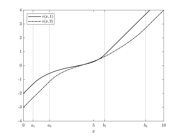
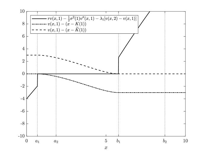
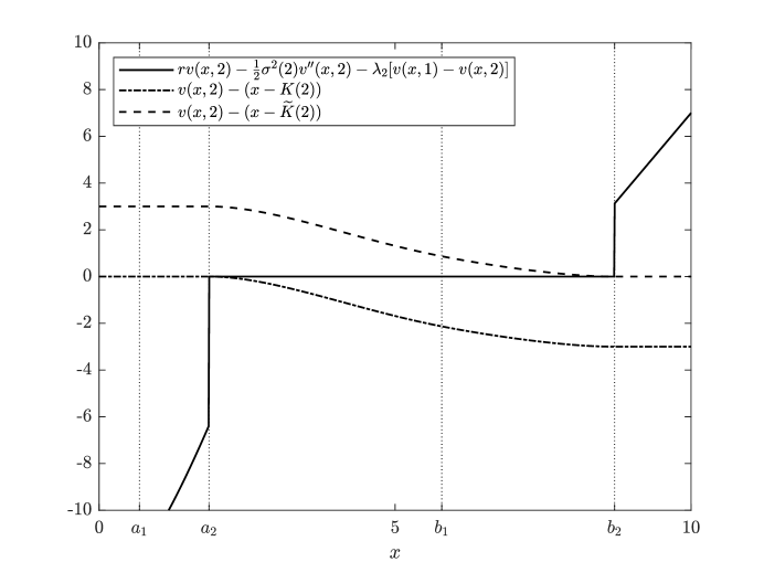
We take $r=3$, $\sigma(1)=2$, $\sigma(2)=4$, $K(1)=2$, $K(2)=3$, $\widetilde{K}(1)=5$, $\widetilde{K}(2)=6$, $\lambda_{1}=2$, $\lambda_{2}=5$ as a set of benchmark parameters and compute the closed-form solutions given by Theorem 3.1. In this case, from (25), the threshold levels are computed to be $(a_{1},a_{2},b_{1},b_{2})=(0.68,1.86,5.79,8.71)$. The value function $v(x,i)$, $i\in\{1,2\}$, is plotted in Figure 1. Moreover, Figures 2 and 3 verify that $v(x,i)$, $i\in\{1,2\}$, satisfies the conditions of the verification theorem (Theorem 2.1). Next, we examine the monotonicity of the threshold levels $(a_{1},a_{2},b_{1},b_{2})$ with respect to the model parameters $\sigma(i)$, $K(i)$, $\widetilde{K}(i)$, $i\in\mathcal{M}$.

Figure 1: Value function $v(x,i)$, $i\in\{1,2\}$

Figure 2: Verification theorem for $v(x,1)$

Figure 3: Verification theorem for $v(x,2)$

First, we vary $\sigma(1)$ and keep all other parameters fixed. The resulting $(a_{1},a_{2},b_{1},b_{2})$ are listed in Table 2. From Table 2, we see that $a_{1}$ decreases and $b_{1}$ increases as $\sigma(1)$ increases, while $a_{2}$ and $b_{2}$ remain nearly unchanged. This is because $\sigma(1)$ is the volatility of $X_{t}$ when the Markov chain $\alpha_{t}$ is at regime 1. The larger of $\sigma(1)$, the farther $X_{t}$ can reach, which leads to a lower $a_{1}$ for Player 1 and a higher $b_{1}$ for Player 2 to achieve a better payoff. On the other hand, we vary $\sigma(2)$ and the corresponding results are similar and listed in Table 3.

Table 2: Dependence on $\sigma(1)$

$\sigma(1)$	2.0	2.5	3.0	3.5	4.0
$a_{1}$	0.68	0.51	0.34	0.17	0.01
$a_{2}$	1.86	1.84	1.82	1.81	1.79
$b_{1}$	5.79	5.95	6.11	6.27	6.43
$b_{2}$	8.71	8.71	8.71	8.72	8.72

Table 3: Dependence on $\sigma(2)$

$\sigma(2)$	4.0	4.5	5.0	5.5	6.0
$a_{1}$	0.68	0.68	0.68	0.67	0.67
$a_{2}$	1.86	1.73	1.61	1.49	1.37
$b_{1}$	5.79	5.80	5.80	5.81	5.82
$b_{2}$	8.71	8.85	8.99	9.13	9.27

Then, we vary $K(1)$ and keep all other parameters fixed. The resulting $(a_{1},a_{2},b_{1},b_{2})$ are listed in Table 4. Table 4 suggests that $a_{1}$ increases if $K(1)$ increases, while $a_{2}$, $b_{1}$, $b_{2}$ have no obvious variation. Note that $a_{1}-K(1)$ is the payoff for Player 1 if it stops when the Markov chain is at regime 1. Player 1 is the one who wants to minimize (2), so a larger $K(1)$ means a bigger stopping reward, which encourages Player 1 to lock down profit by stopping earlier (i.e., a higher $a_{1}$). On the other hand, we vary $K(2)$ and the corresponding results are similar and listed in Table 5.

Table 4: Dependence on $K(1)$

$K(1)$	2.0	2.1	2.2	2.3	2.4
$a_{1}$	0.68	0.84	1.00	1.16	1.31
$a_{2}$	1.86	1.85	1.84	1.83	1.82
$b_{1}$	5.79	5.79	5.79	5.79	5.79
$b_{2}$	8.71	8.71	8.71	8.71	8.71

Table 5: Dependence on $K(2)$

$K(2)$	3.0	3.1	3.2	3.3	3.4
$a_{1}$	0.68	0.62	0.56	0.49	0.43
$a_{2}$	1.86	1.97	2.08	2.19	2.30
$b_{1}$	5.79	5.78	5.78	5.78	5.77
$b_{2}$	8.71	8.71	8.71	8.70	8.70

Finally, we vary $\widetilde{K}(1)$ and keep all other parameters fixed. The resulting $(a_{1},a_{2},b_{1},b_{2})$ are listed in Table 6. Table 6 implies that $b_{1}$ increases in $\widetilde{K}(1)$, while $a_{1}$, $a_{2}$, $b_{2}$ fluctuate slightly. This is due to that a larger $\widetilde{K}(1)$ means a bigger stopping cost for Player 2 when the Markov chain is at regime 1, which in turn needs to be compensated by a higher stopping level (i.e., a higher $b_{1}$). On the other hand, we vary $\widetilde{K}(2)$ and the corresponding results are similar and listed in Table 7.

Table 6: Dependence on $\widetilde{K}(1)$

$\widetilde{K}(1)$	5.0	5.1	5.2	5.3	5.4
$a_{1}$	0.68	0.68	0.68	0.68	0.68
$a_{2}$	1.86	1.85	1.85	1.84	1.84
$b_{1}$	5.79	5.89	6.00	6.11	6.21
$b_{2}$	8.71	8.55	8.40	8.26	8.12

Table 7: Dependence on $\widetilde{K}(2)$

$\widetilde{K}(2)$	6.0	6.1	6.2	6.3	6.4
$a_{1}$	0.68	0.68	0.68	0.68	0.68
$a_{2}$	1.86	1.86	1.86	1.86	1.86
$b_{1}$	5.79	5.79	5.79	5.78	5.78
$b_{2}$	8.71	8.97	9.22	9.49	9.75

4.2 Reduction

In the case with no regime switching, the state process $X\in R$ is described by

$$X_{t}=x+\sigma W_{t},\quad t\geq 0,$$

where $\sigma$ is a positive constant. The objective functional for Player 1 to minimize and Player 2 to maximize is given by

$$J(x;\tau_{1},\tau_{2})=E[e^{-r\tau_{1}}(X_{\tau_{1}}-K)1_{\{\tau_{1}<\tau_{2}\}}+e^{-r\tau_{2}}(X_{\tau_{2}}-\widetilde{K})1_{\{\tau_{2}\leq\tau_{1}\}}],$$

where $K$ and $\widetilde{K}$ are two constants with $K<\widetilde{K}$. As the case with regime switching, we would like to find a threshold-type Nash equilibrium consists of two levels $a<b$ such that Player 1 will stop if $X_{t}$ falls below $a$ and Player 2 will stop if $X_{t}$ goes above $b$. For convenience, we list the derivation sketch of determining the threshold levels $a$ and $b$ and the corresponding value function $v(x)$ as follows, which is also based on Theorem 2.1 but with no regime switching.

Consider $v(x)$ on the continuation region $(a,b)$:

$$rv(x)-\frac{1}{2}\sigma^{2}v^{\prime\prime}(x)=0.$$

The solution is

$$v(x)=A_{1}e^{\beta_{1}x}+A_{2}e^{\beta_{2}x},$$

where $\beta_{1},\beta_{2}$ satisfy the following equation:

$$r-\frac{1}{2}\sigma^{2}\beta^{2}=0,$$

which has two real roots:

$$\beta_{1,2}=\pm\sqrt{\frac{2r}{\sigma^{2}}}.$$

On $(-\infty,a)$, Player 1 stops such that

$$v(x)=x-K.$$

On $(b,\infty)$, Player 2 stops such that

$$v(x)=x-\widetilde{K}.$$

By applying the smooth-fit principle to $v(x)$ at $a$,

$$a-K=A_{1}e^{\beta_{1}a}+A_{2}e^{\beta_{2}a},$$ (26)

$$1=A_{1}\beta_{1}e^{\beta_{1}a}+A_{2}\beta_{2}e^{\beta_{2}a},$$ (27)

and at $b$,

$$A_{1}e^{\beta_{1}b}+A_{2}e^{\beta_{2}b}=b-\widetilde{K},$$ (28)

$$A_{1}\beta_{1}e^{\beta_{1}b}+A_{2}\beta_{2}e^{\beta_{2}b}=1.$$ (29)

From (26) and (27), we have

$$\left[\begin{array}[]{c}a-K\\ 1\\ \end{array}\right]=\left[\begin{array}[]{cc}e^{\beta_{1}a}&e^{\beta_{2}a}\\ \beta_{1}e^{\beta_{1}a}&\beta_{2}e^{\beta_{2}a}\\ \end{array}\right]\left[\begin{array}[]{c}A_{1}\\ A_{2}\\ \end{array}\right].$$

Then,

$$\left[\begin{array}[]{c}A_{1}\\ A_{2}\\ \end{array}\right]=\left[\begin{array}[]{cc}e^{\beta_{1}a}&e^{\beta_{2}a}\\ \beta_{1}e^{\beta_{1}a}&\beta_{2}e^{\beta_{2}a}\\ \end{array}\right]^{-1}\left[\begin{array}[]{c}a-K\\ 1\\ \end{array}\right].$$ (30)

From (28) and (29), we have

$$\left[\begin{array}[]{c}b-\widetilde{K}\\ 1\\ \end{array}\right]=\left[\begin{array}[]{cc}e^{\beta_{1}b}&e^{\beta_{2}b}\\ \beta_{1}e^{\beta_{1}b}&\beta_{2}e^{\beta_{2}b}\\ \end{array}\right]\left[\begin{array}[]{c}A_{1}\\ A_{2}\\ \end{array}\right].$$

Then,

$$\left[\begin{array}[]{c}A_{1}\\ A_{2}\\ \end{array}\right]=\left[\begin{array}[]{cc}e^{\beta_{1}b}&e^{\beta_{2}b}\\ \beta_{1}e^{\beta_{1}b}&\beta_{2}e^{\beta_{2}b}\\ \end{array}\right]^{-1}\left[\begin{array}[]{c}b-\widetilde{K}\\ 1\\ \end{array}\right].$$ (31)

It follows from (30) and (31) that

$$\left[\begin{array}[]{cc}e^{\beta_{1}a}&e^{\beta_{2}a}\\ \beta_{1}e^{\beta_{1}a}&\beta_{2}e^{\beta_{2}a}\\ \end{array}\right]^{-1}\left[\begin{array}[]{c}a-K\\ 1\\ \end{array}\right]=\left[\begin{array}[]{cc}e^{\beta_{1}b}&e^{\beta_{2}b}\\ \beta_{1}e^{\beta_{1}b}&\beta_{2}e^{\beta_{2}b}\\ \end{array}\right]^{-1}\left[\begin{array}[]{c}b-\widetilde{K}\\ 1\\ \end{array}\right],$$ (32)

from which we can solve $a$ and $b$. Then, $A_{1}$ and $A_{2}$ can be represented by (30) or (31).

We consider the following two sets of parameters and numerically compute the corresponding threshold levels and value functions.

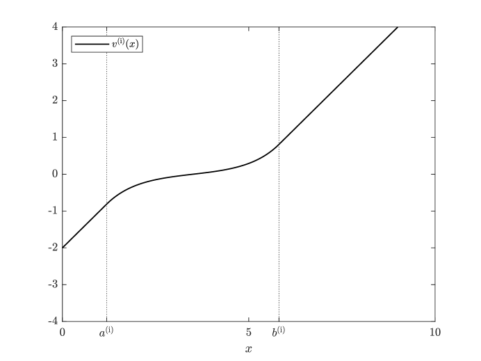
Case (i). Let $r=3$, $\sigma=\sigma(1)=2$, $K=K(1)=2$, $\widetilde{K}=\widetilde{K}(1)=5$. In this case, from (32), the threshold levels are computed to be $(a^{{\rm(i)}},b^{{\rm(i)}})=(1.19,5.81)$. The corresponding value function $v^{{\rm(i)}}(x)$ is plotted in Figure 4.

Figure 4: Value function $v^{({\rm i})}(x)$

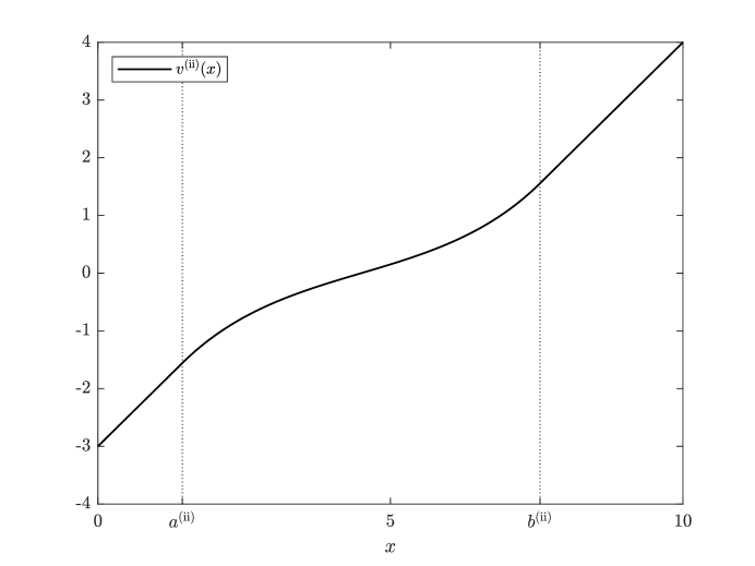
Case (ii). Let $r=3$, $\sigma=\sigma(2)=4$, $K=K(2)=3$, $\widetilde{K}=\widetilde{K}(2)=6$. In this case, from (32), the threshold levels are computed to be $(a^{{\rm(ii)}},b^{{\rm(ii)}})=(1.44,7.56)$. The corresponding value function $v^{{\rm(ii)}}(x)$ is plotted in Figure 5.

Figure 5: Value function $v^{({\rm ii})}(x)$

In addition, we can also verify numerically that $v^{{\rm(i)}}(x)$ and $v^{{\rm(ii)}}(x)$ satisfy the conditions of Theorem 2.1. We omit the details for simplicity of presentation.

5 Concluding remarks

There are three main contributions made in this paper. Firstly, a verification theorem as a sufficient criterion for Nash equilibriums is established, which involves a set of VIs and an appropriate regularity requirement. Secondly, the smooth-fit principle is further developed for our stopping game problem with regime switching to solve the VIs and derive a suitable system of algebraic equations. Thirdly, various numerical experiments are included to demonstrate the theoretical results with reasonable remarks.

This paper, we believe, has posed more questions than answers. The problem formulation considered in this paper is a simple but illustrative one, extensions to more general problems may open up a new avenue for optimal stopping theory. On the other hand, the stopping game problem with regime switching should have a wide range of applications in many fields, such as finance, management, engineering, and so on. These topics in practice will be considered in our future study.

References

• [1] R. Aïd, M. Basei, G. Callegaro, L. Campi, T. Vargiolu, Nonzero-sum stochastic differential games with impulse controls: A verification theorem with applications, Math. Oper. Res., 45 (2020), 205-232.
• [2] K. Akdim, Y. Ouknine, I. Turpin, Variational inequalities for combined control and stopping game, Stoch. Anal. Appl., 24 (2006), 1263-1284.
• [3] A. Bensoussan, A. Friedman, Nonzero-sum stochastic differential games with stopping times and free boundary problems, Trans. Amer. Math. Soc., 231 (1977), 275-327.
• [4] T. De Angelis, G. Ferrari, J. Moriarty, Nash equilibria of threshold type for two-player nonzero-sum games of stopping, Ann. Appl. Probab., 28 (2018), 112-147.
• [5] A. Friedman, Stochastic games and variational inequalities, Arch. Rational Mech. Anal., 51 (1973), 321-346.
• [6] X. Guo, Q. Zhang, Closed-form solutions for perpetual American put options with regime switching, SIAM J. Appl. Math., 64 (2004), 2034-2049.
• [7] X. Guo, Q. Zhang, Optimal selling rules in a regime switching market, IEEE Trans. Automat. Control, 50 (2005), 1450-1455.
• [8] S. Lv, Z. Wu, Q. Zhang, The Dynkin game with regime switching and applications to pricing game options, Ann. Oper. Res., 313 (2022), 1159-1182.
• [9] H. P. McKean, A free boundary problem for the heat equation arising from a problem in mathematical economics, Industrial Management Rev., 6 (1965) 32-39.
• [10] B. Øksendal, Stochastic Differential Equations: An Introduction with Applications, 6th ed., Springer-Verlag, Berlin, 2003.
• [11] H. Pham, Continuous-Time Stochastic Control and Optimization with Financial Applications, Springer-Verlag, Berlin, 2009.
• [12] G. Yin, Q. Zhang, Continuous-Time Markov Chains and Applications: A Two-Time-Scale Approach, 2th ed., Springer, New York, 2013.
• [13] G. Yin, C. Zhu, Hybrid Switching Diffusions: Properties and Applications, Springer, New York, 2010.
• [14] Q. Zhang, Stock trading: An optimal selling rule, SIAM J. Control Optim., 40 (2001), 64-87.
• [15] Q. Zhang, X. Y. Zhou, Valuation of stock loans with regime switching, SIAM J. Control Optim., 48 (2009), 1229-1250.