Generalized Honeycomb-structured Materials in the Subwavelength Regime

Abstract

Honeycomb structures lead to conically degenerate points on the dispersion surfaces. These spectral points, termed as Dirac points, are responsible for various topological phenomena. In this paper, we investigate the generalized honeycomb-structured materials, which have six inclusions in a hexagonal cell. We obtain the asymptotic band structures and corresponding eigenstates in the subwavelength regime using the layer potential theory. Specifically, we rigorously prove the existence of the double Dirac cones lying on the 2nd-5th bands when the six inclusions satisfy an additional symmetry. This type of inclusions will be referred to as super honeycomb-structured inclusions. Two distinct deformations breaking the additional symmetry, contraction and dilation, are further discussed. We prove that the double Dirac cone disappears, and a local spectral gap opens. The corresponding eigenstates are also obtained to show the topological differences between these two deformations. Direct numerical simulations using finite element methods agree well with our analysis.

35C15, 35C20, 35P15, 35B40, 45M05

1 Introduction

The last two decades have witnessed a vast development in topological materials admitting various intriguing phenomena [24, 26, 29, 30], which are rooted in the symmetries of the materials. A typical example is the graphene-like materials that possess the honeycomb structure. And many experimental and theoretical achievements have been made to realize and understand its related novel phenomena [23, 25, 28, 32]. Due to the underlying geometric symmetries, the honeycomb-structured materials guarantee the existence of Dirac cones in the dispersion surfaces, where two adjacent bands touch each other conically. Such degeneracy carries topology indices, which lead to many topologically protected behaviors [27]. Recently, Wu and Hu proposed a dielectric material with a generalized honeycomb structure [33]. This periodic structure has six inclusions inside a hexagonal cell such that the crystal is $\pi/3$-rotation invariant. Based on this structure, high-order Chern topological states are realized [35].

From the mathematical aspects, much progress has been made on honeycomb-structured materials. The pioneering work by Fefferman and Weinstein provided the first rigorous justifications for the existence of Dirac points on the dispersion surfaces of the two-dimensional Schrödinger operator with honeycomb lattice potentials [17]. Following their framework, LeeThorp et al. extended the existence of Dirac points to general elliptic operators with certain honeycomb symmetries [27]. Besides, other issues are investigated based on honeycomb structures, such as the existence of topologically protected edge states [15, 19], conical diffractions of wave-packet dynamics associated with Dirac points [18], and so on. Different types of conical degenerate spectrum points, such as Weyl points in three-dimensional systems, have also been demonstrated with similar approaches [22]. In discrete setups, tight-binding models are usually used. Wallace [32] first obtained the conical degenerate singularity of the discrete honeycomb lattices. Many people have extensively investigated the discrete models with honeycomb lattices and the connections with their continuous versions. See [2, 16] to name a few.

Recently, Ammari and his collaborators successfully applied the integral equation approach to investigate the Helmholtz systems with piece-wise constant material weights. Motivated by the Minnaert resonances for acoustic waves [8, 11], they apply the Gohberg-Segal theory and layer potential theory [10, 12] to rigorously prove the presence of Dirac points in subwavelength frequencies for honeycomb-structured materials. They paved the way to understanding dielectric or acoustic materials in subwavelength regimes. Many other exciting results are also proved on the edge states[7], periodically driven systems[3], and so on.

In this paper, we shall investigate the generalized honeycomb-structured materials proposed by Wu and Hu[33]. To our knowledge, most results are restricted to numerical simulations of the dispersion surfaces. Very few mathematical analyses have been done. A previous result studied the Schrödinger operator equipped with specific potentials possessing symmetries similar to generalized honeycomb structures[13]. They rigorously proved the existence of double Dirac cones using Fefferman and Weinstein’s framework[17]. Dielectric or acoustic materials with generalized honeycomb-structured inclusions have not been mathematically investigated. This paper aims to give a mathematical theory for the dispersion surfaces and associated eigenfunctions of generalized honeycomb-structured materials in the subwavelength regimes. Specifically, we shall prove the existence of double Dirac cones at the $\Gamma$ point (the origin) of the Brillouin zone when the inclusions have additional symmetries. Two deformations to break this symmetry are illustrated, and we prove the absence of the double Dirac cones and the occurrence of a local spectral gap. Corresponding eigenfunctions are obtained to show the topological difference between the two symmetry-breaking modifications to the materials. This topological difference is used to realize topologically protected edge states which have been experimentally realized [34] and will be analyzed in our future work.

Our approach is inspired by the layer potential representations for the eigenfunctions and associated eigenvalues for honeycomb lattices with two inclusions in a diamond cell [9]. Recasting the eigenvalue problems into a characteristic value problem of a boundary integral operator, we immediately encounter the singularity and the lack of invertibility of the single layer operator since the conical degeneracy of interest occurs in the subwavelength frequency at the $\Gamma$ point. Thus considerable modifications to the routine reduction [9] will be made to conquer the obstacles. Motived by the results in[6], we rescale the quasi-periodic Bloch wave vector $\alpha$. Consequently, a uniformly valid asymptotic approximation to the singular potentials is obtained. Once the periodic capacitance matrix is well defined, we can associate its eigenvalue and eigenvectors to the subwavelength frequencies and corresponding eigenfunctions asymptotically. We numerically compute the Bloch frequencies and corresponding eigenfunctions using finite element methods. The numerical results agree well with our analysis.

The paper is organized as follows. In Section 2, we first formulate the problem and review some well-known results on the quasi-periodic Green’s functions and related layer potentials. In Section 3, the periodic capacitance matrix is defined by asymptotic expansion of Green’s function. From this end, we study the asymptotic behaviors of the eigenvalue problem. Given the additional symmetries, the existence of a double Dirac point at $\Gamma$ is rigorously proven in Section 4. We will also briefly discuss how the two deformations affect the band structures and eigenfunctions. A direct numerical simulation based on a finite element method is presented in Section 5.

2 Problem Formulation and Preliminaries

In this section, the eigenvalue problem of generalized honeycomb-structured materials is formulated. Following the notations in [10], we briefly review the layer potential theory for periodic inclusions.

2.1 Generalized Honeycomb-structured Inclusions

Consider the set of lattice points $\Lambda\triangleq\{n_{1}l_{1}+n_{2}l_{2}:n_{1},n_{2}\in\mathbb{Z}\}$, where $l_{1},l_{2}$ are vectors in $\mathbb{R}^{2}$ given by

(1) $$l_{1}=(1/2,-\sqrt{3}/2)^{T},\quad l_{2}=(1/2,\sqrt{3}/2)^{T}.$$

The parallelogram region $\{sl_{1}+tl_{2}:s,t\in[0,1]\}$ can be reformed to the the hexagonal unit cell enclosed by $A,B,C,D,E,F$ by periodicity, where $A=(-l_{1}+l_{2})/3,B=(l_{1}+2l_{2})/3,C=(2l_{1}+l_{2})/3,D=-A,E=-B,F=-C$. We denote the hexagonal region by $Y$. See Figure 1.

We introduce the following three matrices $R$, $T_{x}$ and $T_{y}$,

(2) $$R\triangleq\begin{pmatrix}\frac{1}{2}&\frac{\sqrt{3}}{2}\\ -\frac{\sqrt{3}}{2}&\frac{1}{2}\end{pmatrix},\quad T_{x}\triangleq\begin{pmatrix}1&0\\ 0&-1\end{pmatrix},\quad T_{y}\triangleq\begin{pmatrix}-1&0\\ 0&1\end{pmatrix}.$$

They correspond to the $-\pi/3$-rotation matrix, the reflection with respect to x-axis and y-axis. And we assume that $D_{0}$ is a connected open domain containing the origin $O$ with piece-wise smooth boundary such that:

• $R^{2}D_{0}=D_{0},\quad T_{x}D_{0}=D_{0};$

• $\operatorname{diam}(D_{0})\triangleq\sup_{x,y\in D_{0}}\|x-y\|_{\mathbb{R}^{2}}<1/4.$ Here $\|\cdot\|_{\mathbb{R}^{2}}$ denotes the usual Euclidean norm.

By translations and rotations we define $\{D_{j}\}_{j=1}^{6}$ by

$$D_{1}\triangleq D_{0}-\frac{1}{3}(1+\sigma)l_{1},\quad D_{j}\triangleq R^{j-1}D_{1},\;j=2,3,\ldots,6.$$

Here and thereafter the parameter $\sigma$ is chosen such that $D\Subset Y$ and has six connect components. It is easy to see that the point $P_{i}$ is contained in $D_{i}$, where $P_{1}=(1+\sigma)l_{1}/3$, $P_{j}=R^{j-1}P_{1}$ for $j=2,3,\ldots 6$. Further we let $D\triangleq\cup_{j=1}^{6}D_{j}$. And its periodic tiling $D_{per}$ can be defined by

(3) $$D_{per}=\{x+n_{1}l_{1}+n_{2}l_{2}:x\in D,n_{1},n_{2}\in\mathbb{Z}\}.$$

In this article, the periodic inclusions $D_{per}$ will be called the generalized honeycomb-structured inclusions. Specifically for $\sigma=0$, the inclusions $D_{per}$ will be called the super honeycomb-structured inclusions. When $\sigma>0(<0)$, we will say that the inclusions are contracted(dilated). An example of $D_{per}$ when $\sigma=0$ is illustrated in Figure 1. While in Figure 2 we illustrate the inclusions when they are either contracted or dilated. The corresponding super honeycomb-structured inclusions in unit cell are plotted in dash lines.

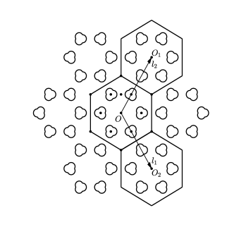
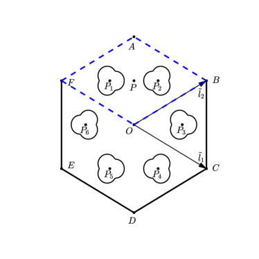
Figure 1: Left: honeycomb-structured inclusions. The unit cell $Y$ is enclosed in black bold line. Right: illustration of the unit cell $Y$. The region $\tilde{Y}$ is enclosed in blue dash lines.

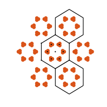
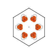
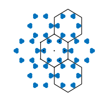
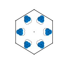
Figure 2: Left: illustrations of the generalized honeycomb-structured inclusions and the unit cell when the inclusions are contracted. Here $\sigma$ is negative. Right: illustration of the generalized honeycomb-structured inclusions and the unit cell when the inclusions are dilated. Here $\sigma$ is positive. The corresponding super honeycomb-structured inclusions are plotted in dash lines.

Through simple calculations, one can verify that the generalized honeycomb-structured inclusions is invariant under the $\pi/3$-rotation at $O$ and the reflection with respect to y-axis, which is equivalent to $RD_{per}=D_{per},T_{y}D_{per}=D_{per}$.

The dual lattice of $\Lambda$ is defined as $\Lambda^{\prime}\triangleq\{n_{1}k_{1}+n_{2}k_{2}:n_{1},n_{2}\in\mathbb{Z}\},$ with vectors $k_{1}$ and $k_{2}$ satisfying

(4) $$k_{i}\cdot l_{j}=2\pi\delta_{ij},\quad i,j=1,2.$$

The Brillouin zone is defined by $Y^{\prime}\triangleq\mathbb{R}^{2}/\Lambda^{\prime}$. For convenience we choose the representation $Y^{\prime}\simeq\{sk_{1}+tk_{2}:s,t\in[0,1)\}.$

2.2 Problem Formulation

Given the geometry properties, we now define the eigenvalue problem in the generalized honeycomb-structured crystal.

$$\nabla\cdot(\frac{1}{\rho(x)}\nabla u(x))=\frac{\omega^{2}}{\kappa(x)}u(x),\quad u(x)\in\mathbb{L}^{2}(\mathbb{R}^{2}).$$

Here the material weights $\rho(x),\kappa(x)$ are given by

$$\rho(x)\triangleq\rho_{0}\chi_{{}_{\mathbb{R}^{2}\backslash D_{per}}}(x)+\rho_{1}\chi_{{}_{D_{per}}}(x),\quad\kappa(x)\triangleq\kappa_{0}\chi_{{}_{\mathbb{R}^{2}\backslash D_{per}}}(x)+\kappa_{1}\chi_{{}_{D_{per}}}(x),$$

where $\chi_{{}_{D_{per}}}$ and $\chi_{{}_{\mathbb{R}^{2}\backslash D_{per}}}$ are the characteristic functions of $D_{per}$ and $\mathbb{R}^{2}\backslash D_{per}$. And $\rho_{0},\kappa_{0}$ and $\rho_{1},\kappa_{1}$ denote the densities and bulk moduli outside and inside the inclusions, respectively. We introduce

$$v_{0}\triangleq\sqrt{\frac{\kappa_{0}}{\rho_{0}}},\;v_{1}\triangleq\sqrt{\frac{\kappa_{1}}{\rho_{1}}},\;k_{0}\triangleq\frac{\omega}{v_{0}},\;k_{1}\triangleq\frac{\omega}{v_{1}},\;\delta\triangleq\frac{\rho_{1}}{\rho_{0}}.$$

By Floquet-Bloch decomposition, the eigenvalue problem in $\mathbb{L}^{2}(\mathbb{R}^{2})$ is reduced to the quasi-periodic eigenvalue problem for all $\alpha\in Y^{\prime}$. Combining the jump relations, we can formulate the $\alpha$-quasi-periodic problem for $\alpha\in Y^{\prime}$:

(5) $$\left\{\begin{aligned} &\Delta u+k_{0}^{2}u=0,\quad x\in\mathbb{R}^{2}\backslash\overline{D_{per}},\\ &\Delta u+k_{1}^{2}u=0,\quad x\in D_{per},\\ &u|_{+}-u|_{-}=0,\quad y\in\partial D_{per},\\ &\delta\left.n_{y}\cdot\nabla u\right|_{+}-\left.n_{y}\cdot\nabla u\right|_{-}=0,\quad y\in\partial D_{per},\\ &u(x+l)=\mathrm{e}^{\mathrm{i}\alpha\cdot l}u(x),\quad\forall x\in\mathbb{R}^{2},l\in\Lambda.\end{aligned}\right.$$

Here, $n_{y}\cdot\nabla u$ denotes the normal derivative of $u$ at $y\in\partial D_{per}$, and the subscripts $+$ and $-$ denotes the limit from outside and inside of $D_{per}$. For any $\alpha\in Y^{\prime}$, the eigenvalue problem (5) has discrete eigenvalues $\{\omega^{2}_{n}(\alpha,\sigma)\}$ that tend to infinity as $n\to\infty$.

The parameter $\delta$ denotes the contrast in the density and we assume that $\delta$ is small, while the wave speed are comparable and of $\mathcal{O}(1)$, i.e.,

$$0<\delta\ll 1\quad\text{and}\quad v_{0},v_{1}=\mathcal{O}(1).$$

In this article, we say that a frequency $\omega$ is a subwavelength frequency if $\omega^{2}=\mathcal{O}(\delta)$. And the problem of interest is the subwavelength frequency when the quasi-periodicity vector $\alpha$ is close to the $\Gamma$ point, namely the point $\alpha=0$. We are also interested in the behavior of band structures when the inclusions are contracted or dilated.

Our main theorems are Theorem 3.7 and Theorem 4.10. We rigorously prove the existence of double Dirac point at $\alpha=0$ when the inclusions $D_{per}$ are super honeycomb-structured inclusions. Then we study the asymptotic behavior of band structure when the inclusions are contracted or dilated, that is to say, when $\sigma<0$ or $\sigma>0$. And we show that the second and third bands will detach from the fourth and fifth bands.

Remark 2.1.

Notice that the subwavelength regime is different from the tight binding regime [1, 16] or the high contrast regime [14].

2.3 Green’s Functions and Layer Potentials

Consider the quasi-periodic Green’s function $G^{\alpha,\omega}$ defined by the spectral representation

(6) $$G^{\alpha,\omega}(x)=\frac{1}{|Y|}\sum_{q\in\Lambda^{\prime}}\frac{\mathrm{e}^{\mathrm{i}(\alpha+q)\cdot x}}{\omega^{2}-|\alpha+q|^{2}},$$

where $\omega\neq|\alpha+q|$ for all $q\in\Lambda^{\prime}$. If both $\omega$ and $\alpha$ are zero, we define the periodic Green’s function $G^{0,0}$ by

(7) $$G^{0,0}(x)=\frac{1}{|Y|}\sum_{q\in\Lambda^{\prime}\backslash\{0\}}-\frac{\mathrm{e}^{\mathrm{i}q\cdot x}}{|q|^{2}}.$$

Now we define the quasi-periodic single layer potential of the density function $\phi\in\mathbb{L}^{2}(\partial D)$ as

(8) $$\mathcal{S}_{D}^{\alpha,\omega}[\phi]\triangleq\int_{\partial D}G^{\alpha,\omega}(x-y)\phi(y)d\sigma(y).$$

Then the following well-known jump relations are implied directly [10]

(9) $$\left.n_{y}\cdot\nabla\mathcal{S}_{D}^{\alpha,\omega}[\phi]\right|_{\pm}=\pm\frac{\phi(y)}{2}+(\mathcal{K}^{-\alpha,\omega}_{D})^{\ast}[\phi](y),$$

where the Neumann-Poincaré operator $(\mathcal{K}_{D}^{-\alpha,\omega})^{\ast}$ is defined by

(10) $$(\mathcal{K}_{D}^{-\alpha,\omega})^{\ast}[\varphi](x)\triangleq\operatorname{p.v.}\int_{\partial D}n_{x}\cdot\nabla G^{\alpha,\omega}(x-y)\varphi(y)d\sigma(y),\quad x\in\partial D.$$

Its $\mathbb{L}^{2}(\partial D)$ adjoint operator $\mathcal{K}_{D}^{\alpha,\omega}$ is given by

(11) $$\mathcal{K}_{D}^{\alpha,\omega}[\varphi](x)\triangleq\operatorname{p.v.}\int_{\partial D}n_{y}\cdot\nabla G^{\alpha,\omega}(x-y)\varphi(y)d\sigma(y),\quad x\in\partial D.$$

One can prove that the single layer potential is invertible when it is regarded as an operator $\mathcal{S}_{D}^{\alpha,\omega}:\mathbb{L}^{2}(\partial D)\to\mathbb{H}^{1}(\partial D)$ when $\omega$ is small enough and $\omega\neq|\alpha+q|$ for all $q\in\Lambda^{\prime}$, see Lemma 3.1 in [6].

2.4 Integral Equation Formulation

By layer potential theory, the original problem (5) can be recast into an integral equation problem. We represent the solution by single layer potentials if $(\omega,\alpha)$ is nonzero:

(12) $$u(x)=\left\{\begin{aligned} &\mathcal{S}^{\alpha,k_{b}}_{D}[\phi](x),\quad x\in D,\\ &\mathcal{S}^{\alpha,k_{0}}_{D}[\psi](x),\quad x\in Y\backslash\overline{D},\end{aligned}\right.$$

Here $\phi,\psi\in\mathbb{L}^{2}(\partial D)$ and are determined by following equations:

(13) $$\left\{\begin{aligned} &\mathcal{S}^{\alpha,k_{b}}_{D}[\phi](y)=\mathcal{S}_{D}^{\alpha,k_{0}}[\psi](y)\\ &-\frac{\phi(y)}{2}+(\mathcal{K}^{-\alpha,k_{b}}_{D})^{\ast}[\phi](y)=\delta\left(\frac{\psi(y)}{2}+(\mathcal{K}^{-\alpha,k_{0}}_{D})^{\ast}[\psi](y)\right)\end{aligned}\right.,\quad y\in\partial D.$$

If $(\omega,\alpha)$ is zero, we will prove in the appendix that the harmonic periodic solutions can be represented by single layer potential up to a constant, see the discussions in Appendix B. So the usual procedures (see [9]) to investigate the band structure near $\alpha=0$ fail due to the lack of invertibility of $\mathcal{S}^{0,0}_{D}$. The singularity will also arise when we consider the band structures in subwavelength regime. More importantly, we have to first justify the representation (12) of the eigenfunctions corresponding to subwavelength eigenvalues.

Fortunately, again by the discussions in Appendix B, one only has to take care of constant functions. And the characteristic value problem of the operator $\mathcal{A}^{\alpha,\omega}_{\delta}:(\mathbb{L}^{2}(\partial D))^{2}\to(\mathbb{L}^{2}(\partial D))^{2}$ given by

(14) $$\mathcal{A}^{\alpha,\omega}_{\delta}\begin{pmatrix}\phi\\ \psi\end{pmatrix}\triangleq\begin{Bmatrix}\mathcal{S}^{\alpha,k_{b}}_{D}[\phi]-\mathcal{S}^{\alpha,k_{0}}_{D}[\psi]\\ -\frac{1}{2}\phi+\left(\mathcal{K}^{-\alpha,k_{b}}_{D}\right)^{\ast}[\phi]-\delta\left[\frac{1}{2}\psi+\left(\mathcal{K}^{-\alpha,k_{0}}_{D}\right)^{\ast}[\psi]\right]\end{Bmatrix},$$

is still able to represent the corresponding eigenvalues of (5). Here notice that $\mathcal{A}^{\alpha,\omega}_{\delta}$ is a function of $\omega$, since $k_{0}$ and $k_{b}$ are functions of $\omega$. With this definition, (13) is equivalent to

(15) $$\mathcal{A}^{\alpha,\omega}_{\delta}\begin{pmatrix}\phi\\ \psi\end{pmatrix}=\begin{pmatrix}0\\ 0\end{pmatrix}.$$

By the properties of elliptic eigenvalue problem, the above integral equations has non-trivial solutions for some discrete frequencies $\omega$. And they can be viewed as the characteristic values of the operator-valued analytic function $\mathcal{A}^{\alpha,\omega}_{\delta}:\mathbb{C}\to[(\mathbb{L}^{2}(\partial D))^{2}\to(\mathbb{L}^{2}(\partial D))^{2}]$.

3 Asymptotic Behavior of Band Structure

This section is devoted to characterizing the band structure in subwavelength regime of generalized honeycomb-structured inclusions $D$. To this end, we first describe the asymptotic behavior of Green’s functions when both $\omega$ and $|\alpha|$ are small. Then by properly defining the periodic capacitance matrix $\mathbf{C}^{0}$, we obtain the asymptotic behavior of band structures near $\alpha=0$.

3.1 Asymptotic Expansion of Green’s Function

In order to study the asymptotic behavior near $\alpha=0$, we set $\alpha=\omega^{2}\alpha_{0}$ for some $\alpha_{0}\in Y^{\prime}$ independent of $\omega$. When $\omega\to 0$ and $\alpha\neq 0$, we have, from (6),

(16) $$G^{\omega^{2}\alpha_{0},\omega}(x)=\frac{1}{|Y|}\Big{(}\frac{1}{\omega^{2}}+\mathrm{i}\alpha_{0}\cdot x+|\alpha_{0}|^{2}\Big{)}+G^{0,0}(x)+\omega^{2}G^{\alpha_{0}}_{2}+o(\omega^{2}).$$

Consequently we obtain an $\mathcal{O}(\omega^{2})$ approximation of $\mathcal{S}^{\omega^{2}\alpha_{0},\omega}_{D}$:

(17) $$\begin{aligned} \hat{\mathcal{S}}^{\omega^{2}\alpha,\omega}_{D}[\varphi](x)&\triangleq\mathcal{S}_{D}^{0,0}[\varphi](x)+\frac{1}{|Y|}\left(\frac{1}{\omega^{2}}+|\alpha_{0}|^{2}\right)\int_{\partial D}\varphi(y)d\sigma(y)\\ &\quad+\frac{\mathrm{i}}{|Y|}\int_{\partial D}\alpha_{0}\cdot(x-y)\varphi(y)d\sigma(y).\end{aligned}$$

Here $\mathcal{S}^{0,0}_{D}$ denotes the periodic single layer potential associated to $G^{0,0}$. Although the operator $\mathcal{S}^{0,0}_{D}$ is not invertible in general, it can be proved that for small but nonzero $\omega$, the operator $\hat{\mathcal{S}}^{\omega^{2}\alpha,\omega}_{D}$ is invertible [6]. However, the kernel of periodic single layer potential can be characterized following the same spirit of [5, 6]:

Lemma 3.1.

If $\mathcal{S}^{0,0}_{D}[\varphi]=K\chi_{{}_{\partial D}}$ for some constant $K$ and some $\varphi\in\mathbb{L}^{2}_{0}(\partial D)$, then $\varphi\equiv 0$.

Proof 3.2.

By the uniqueness result of the homogeneous Dirichlet problem (see, for example [31]), the function $\mathcal{S}^{0,0}_{D}[\varphi]$ is a constant. Then by (9) we obtain

$$\varphi(y)=n_{y}\cdot\mathcal{S}^{0,0}_{D}[\varphi]|_{+}-n_{y}\cdot\mathcal{S}^{0,0}_{D}[\varphi]|_{-}=0.$$

In the asymptotic expansion formula (16), it is clear that the operator $\hat{\mathcal{S}}_{D}^{\omega^{2}\alpha_{0},\omega}$ has a $\mathcal{O}(\omega^{-2})$ singularity near zero. However, the inverse operator $\left(\hat{\mathcal{S}}^{\omega^{2}\alpha_{0},\omega}_{D}\right)^{-1}$ behaves well near the zero point.

Lemma 3.3.

Given $\alpha_{0}\in Y^{\prime}$ such that $|\alpha_{0}|<1$, the operator-valued function $\left(\hat{\mathcal{S}}^{\omega^{2}\alpha_{0},\omega}_{D}\right)^{-1}$ is holomorphic with respect to $\omega$ in a neighborhood of $\omega=0$.

Proof 3.4.

From the definition (17), we know that $\hat{\mathcal{S}}^{\omega^{2}\alpha_{0},\omega}_{D}$ is a meromorphic
operator-valued function of $\omega$ with a pole at $\omega=0$. Now assuming $\left(\hat{\mathcal{S}}^{\omega^{2}\alpha_{0},\omega}_{D}\right)^{-1}$ is singular as $\omega\to 0$, there exist some $\phi_{\omega}$ depending on $\omega$ such that $||\phi_{\omega}||_{\mathbb{L}^{2}(\partial D)}=1$ while $||\hat{\mathcal{S}}^{\omega^{2}\alpha_{0},\omega}_{D}[\phi_{\omega}]||_{\mathbb{H}^{1}(\partial D)}=\mathcal{O}(\omega)$. We suppose the $\mathcal{O}(1)$ part of $\phi_{\omega}$ is $\phi_{0}$, which is independent on $\omega$. Then from (17), we have uniformly in $\omega$,

$$\hat{\mathcal{S}}^{\omega^{2}\alpha_{0},\omega}_{D}[\phi_{\omega}](x)=\frac{1}{\omega^{2}|Y|}\int_{\partial D}\phi_{\omega}d\sigma(y)+\mathcal{O}(1).$$

When $|\omega|\ll 1$, we obtain

$$\int_{\partial D}\phi_{0}\,d\sigma(y)=0.$$

Thus we have, $\hat{\mathcal{S}}^{\omega^{2}\alpha,\omega}_{D}[\phi_{0}]=K\chi_{{}_{\partial D}}$ for some constant $K$. It follows from Lemma 3.1 that $\phi_{0}=0$, which contradicts the fact that $||\phi_{\omega}||_{\mathbb{L}^{2}(\partial D)}=\mathcal{O}(1)$.

Now for fixed $\alpha_{0}\in Y^{\prime}$, $\mathbb{H}^{1}(\partial D)\ni f_{r}\sim\mathcal{O}(1)$ and consider the function

(18) $$\hat{\phi}_{j}^{\omega^{2}\alpha_{0},\omega}=\left(\hat{\mathcal{S}}^{\omega^{2}\alpha_{0},\omega}_{D}\right)^{-1}[\chi_{{}_{\partial D_{j}}}+\omega^{2}f_{r}].$$

From Lemma 3.3, we have the following expansion

(19) $$\textstyle\hat{\phi}_{j}^{\omega^{2}\alpha_{0},\omega}=\phi^{\alpha_{0}}_{j,0}+\sum_{k=1}^{+\infty}\omega^{k}\hat{\phi}_{j,k}^{\alpha_{0}}=\phi^{\alpha_{0}}_{j,0}+\omega\hat{\phi}^{\alpha_{0}}_{j,1}+\omega^{2}\hat{\phi}^{\alpha_{0}}_{j,r},$$

as $\omega\to 0$ for some $\phi^{\alpha_{0}}_{j,0},\hat{\phi}^{\alpha_{0}}_{j,1},\hat{\phi}_{j,2}^{\alpha_{0}},\hat{\phi}_{j,r}^{\alpha_{0}}\in\mathbb{L}^{2}(\partial D)$. However, these terms may depend on $f_{r}$. We first state and prove the main properties of $\phi_{j,0}^{\alpha_{0}},\hat{\phi}_{j,1}^{\alpha_{0}},\hat{\phi}_{j,r}^{\alpha_{0}}$ determined by (18) and (19). For every fixed $\alpha_{0}\in Y^{\prime}$ and $f_{r}\in\mathbb{H}^{1}(\partial D)$, we have the following properties:

• The zeroth order term $\phi^{\alpha_{0}}_{j,0}\in\mathbb{L}^{2}_{0}(\partial D)$ is independent of $\alpha_{0}$ and $f_{r}$ and satisfies

  $$\mathcal{S}^{0,0}_{D}[\phi_{j,0}^{\alpha_{0}}]=\chi_{{}_{\partial D_{j}}}-\frac{1}{6}\chi_{{}_{\partial D}};$$

• The first order term $\hat{\phi}^{\alpha}_{j,1}$ vanishes, which is equivalent to $\hat{\phi}^{\alpha}_{j,1}\equiv 0$;

• The following identity holds:

  (20) $$\int_{\partial D}\hat{\phi}^{\alpha_{0}}_{j,r}d\sigma(y)-\mathrm{i}\int_{\partial D}(\alpha_{0}\cdot y)\phi_{j,0}^{\alpha_{0}}\,d\sigma(y)=\frac{|Y|}{6}.$$

Proof 3.5.

Since $\hat{\mathcal{S}}^{\omega^{2}\alpha_{0},\omega}_{D}[\phi_{j}^{\omega^{2}\alpha_{0},\omega}]$ is bounded as $\omega\to 0$, the singular part of $\hat{\mathcal{S}}^{\omega^{2}\alpha_{0},\omega}_{D}$ should vanish on $\phi_{j,0}^{\alpha_{0}}$ and $\hat{\phi}^{\alpha_{0}}_{j,1}$ for any $\alpha_{0}\in Y^{\prime}$. Therefore, we conclude that
$\phi^{\alpha_{0}}_{j,0},\hat{\phi}^{\alpha_{0}}_{j,1}\in\mathbb{L}^{2}_{0}(\partial D)$. From the definition (18), we have $\hat{\mathcal{S}}^{\omega^{2}\alpha_{0},\omega}_{D}[\hat{\phi}_{j}^{\omega^{2}\alpha_{0},\omega}]=\chi_{{}_{\partial D_{j}}}+\omega^{2}f_{r}$. Taking the $\mathcal{O}(1)$ terms gives us the following identity:

(21) $$\chi_{{}_{\partial D_{j}}}=\mathcal{S}^{0,0}_{D}[\phi^{\alpha_{0}}_{j,0}]-\frac{\mathrm{i}}{|Y|}\int_{\partial D}(\alpha_{0}\cdot y)\phi^{\alpha_{0}}_{j,0}d\sigma(y)+\frac{1}{|Y|}\int_{\partial D}\hat{\phi}^{\alpha_{0}}_{j,r}\,d\sigma(y).$$

And thus $\mathcal{S}^{0,0}_{D}[\phi^{\alpha_{0}}_{j,0}]=\chi_{{}_{\partial D_{j}}}+\tilde{K}\chi_{{}_{\partial D}}$ for some constant $\tilde{K}$. By uniqueness result[31], we conclude that $\mathcal{S}^{0,0}_{D}[\phi_{j,0}^{\alpha_{0}}]$ equals to constant in each inclusion $D_{k}$. As a result, we have from (9)

$$\left.n_{y}\cdot\nabla\mathcal{S}^{0,0}_{D}[\phi_{j,0}^{\alpha_{0}}]\right|_{-}=-\frac{1}{2}\phi_{j,0}^{\alpha_{0}}+(\mathcal{K}^{0,0}_{D})^{\ast}[\phi_{j,0}^{\alpha_{0}}]=0.$$

From Appendix A, we have $\tilde{K}=-1/6$ for all $\alpha_{0}\in Y^{\prime}$. So we have proved (i).

To prove (ii), we first substitute $\hat{\phi}_{j}^{\omega^{2}\alpha_{0},\omega}$ into (18) and take the $\mathcal{O}(\omega)$ terms.

(22) $$\mathcal{S}^{0,0}_{D}[\hat{\phi}^{\alpha_{0}}_{j,1}]=\frac{\mathrm{i}}{|Y|}\int_{\partial D}(\alpha_{0}\cdot y)\hat{\phi}^{\alpha_{0}}_{j,1}d\sigma(y)=K\chi_{{}_{\partial D}},$$

for some constant $K$. By Lemma 3.1, the first order term in (19) equals to zero, which finishes the proof of (ii).

As for (iii), we immediately draw the conclusion from (21) and (i).

Now we can define

(23) $$C_{jk}^{0}\triangleq-\int_{\partial D_{k}}\phi_{j,0}^{\alpha_{0}}\,d\sigma(y),$$

And we call the matrix $\mathbf{C}^{0}=(C^{0}_{jk})_{j,k=1}^{6}$ the periodic capacitance matrix. From Section 3.1 we know that the periodic capacitance matrix is independent of $\alpha_{0}$ and $f_{r}$. In the rest of the paper, we omit the superscript in $\phi_{j,0}^{\alpha_{0}}$ and write $\phi_{j,0}$.

Remark 3.6.

One can prove by Green’s identity that the elements of periodic capacitance matrix can be equivalently defined by

(24) $$C_{jk}^{0}=\int_{Y\backslash D}(\nabla\mathcal{S}^{0,0}[\phi_{j,0}]\cdot\nabla\mathcal{S}^{0,0}[\phi_{j,0}])dx,\quad j,k=1,2,\ldots 6.$$

3.2 Asymptotic Behavior of Band Structure

Given the results before, we now state and prove one of the main theorems concerned with the asymptotic behavior of subwavelength frequencies.

Theorem 3.7.

The band functions $\{\omega_{n}^{\alpha}\}_{n=1}^{6}$ are approximated by

$$|\omega_{n}^{\alpha}|^{2}=\frac{6\delta\lambda_{n}v_{b}^{2}}{|D|}+\mathcal{O}(\delta^{2}),$$

uniformly for $|\alpha|<\min(k_{b}^{2},k_{0}^{2})$. Here $|D|$ is the area of the inclusions in the unit cell, and $\lambda_{n}$ are the eigenvalues of the periodic capacitance matrix $\mathbf{C}^{0}$.

Before giving the detailed proof, we first give several lemmas.

Lemma 3.8.

The operator $F^{\alpha_{0}}:\mathbb{L}^{2}(\partial D)\to\mathbb{L}^{2}(\partial D)$ defined by

(25) $$F^{\alpha_{0}}[\phi](y)\triangleq-\frac{\phi}{2}(y)+(\mathcal{K}^{0,0}_{D})^{\ast}[\phi](y)+\frac{\mathrm{i}}{|Y|}\alpha_{0}\cdot n_{y}\int_{\partial D}\phi(z)d\sigma(z),\quad\forall\alpha_{0}\in Y^{\prime},$$

is a Fredholm operator of index zero, with $\ker(F^{\alpha_{0}})=\ker(-\frac{1}{2}\operatorname{Id}+(\mathcal{K}^{0,0}_{D})^{\ast})$.

Proof 3.9.

The operator $F^{\alpha_{0}}$ is a rank-1 perturbation of the Fredholm operator $\ker(-\frac{1}{2}\operatorname{Id}+(\mathcal{K}^{0,0}_{D})^{\ast})$, so it is a Fredholm operator of index zero.

Now for any given $\phi\in\ker(F^{\alpha_{0}})$, we integrate both sides on $\partial D$:

$$\int_{\partial D}\left(-\frac{1}{2}\phi+(\mathcal{K}^{0,0}_{D}[\phi])^{\ast}\right)d\sigma(y)=0,$$

By the mapping property given in Proposition 12.15 in [31], we have $\phi\in\mathbb{L}^{2}_{0}(\partial D)$. Therefore, $\phi$ satisfies

$$-\frac{\phi}{2}+(\mathcal{K}^{0,0}_{D})^{\ast}[\phi]=0,$$

which is equivalent to say $\phi\in\ker(-\frac{1}{2}\operatorname{Id}+(\mathcal{K}^{0,0}_{D})^{\ast})$.

Lemma 3.10.

The operator $\mathcal{K}^{\alpha_{0},0}_{D,2}$ defined by

$$\mathcal{K}^{\alpha_{0},0}_{D,2}[\phi]\triangleq\int_{\partial D}n_{x}\cdot\nabla G^{\alpha_{0}}_{2}(x-y)\phi(y)d\sigma(y),$$

satisfies

(26) $$\int_{\partial D_{k}}\mathcal{K}^{\alpha_{0},0}_{D,2}[\phi]d\sigma(y)=-\int_{D_{k}}\mathcal{S}^{0,0}_{D}[\phi]dx+\mathrm{i}\frac{|D_{k}|}{|Y|}\int_{\partial D}(\alpha_{0}\cdot y)\phi(y)d\sigma(y),$$

for all $\phi\in\mathbb{L}_{0}^{2}(\partial D)$ and $k=1,2,\ldots,6$.

Proof 3.11.

Note that from (9) and (17), we have, for $\phi\in\mathbb{L}^{2}_{0}(\partial D)$

(27) $$\int_{\partial D_{k}}-\frac{1}{2}\phi+(\mathcal{K}^{-\omega^{2}\alpha_{0},\omega}_{D})^{\ast}[\phi]d\sigma(y)=-\omega^{2}\int_{D_{k}}\hat{\mathcal{S}}^{\omega^{2}\alpha_{0},\omega}_{D}[\phi]dx+\mathcal{O}(\omega^{4}).$$

At the same time, we are led to

(28) $$\int_{\partial D_{k}}\bigg{(}-\frac{1}{2}\phi+(\mathcal{K}_{D}^{-\omega^{2}\alpha_{0},\omega})^{\ast}[\phi]\bigg{)}d\sigma(y)=\int_{\partial D_{k}}F^{\alpha_{0}}[\phi](y)d\sigma(y)$$

By the fact that

(29) $$\int_{\partial D_{k}}(\alpha_{0}\cdot n_{y})d\sigma(y)=\int_{D_{k}}\operatorname{div}(\alpha_{0})dx=0,$$

and collecting the above discussions, we obtain, for all $|\omega|\ll 1$,

$$\begin{aligned} \omega^{2}\int_{\partial D_{k}}\mathcal{K}^{\alpha_{0},0}_{D,2}[\phi]d\sigma(y)&=-\omega^{2}\int_{D_{k}}\hat{\mathcal{S}}^{\omega^{2}\alpha_{0},\omega}_{D}[\phi]dx+\mathcal{O}(\omega^{4})\\ &=-\omega^{2}\bigg{\{}\int_{D_{k}}\mathcal{S}^{0,0}_{D}[\phi]dx-\frac{\mathrm{i}}{|Y|}\int_{D_{k}}\bigg{[}\int_{\partial D}(\alpha_{0}\cdot y)\phi(y)d\sigma(y)\bigg{]}dx\bigg{\}}.\end{aligned}$$

The $\mathcal{O}(\omega^{2})$ terms are independent of $\omega$, and they must coincide.

Further, one notes the continuous dependency on $\delta$ of the original problem. There are six Bloch resonant frequencies $\{\omega_{n}^{0}=\omega_{n}^{0}(\delta)\}_{n=1}^{6}$ such that $\{\omega_{n}^{0}(0)=0\}_{n=1}^{6}$ and $\{\omega^{0}_{n}(\delta)\}_{n=1}^{6}$ depends on $\delta$ continuously.

Proof 3.12.

When $\alpha\neq 0$, we can adopt the standard procedure to prove that there exist six Bloch resonant frequency $\{\omega_{n}^{\alpha}=\omega_{n}^{\alpha}(\delta)\}_{n=1}^{6}$ such that $\{\omega_{n}^{\alpha}(0)=0\}_{n=1}^{6}$. See, for example, [9]. By the Lipschitz continuity of the band function with respect of $\alpha$, we claim that $\{\omega_{n}^{0}(0)=0\}_{n=1}^{6}$ and there exist at most six Bloch resonant frequencies when $\alpha=0$.

First, it is clear that $\omega^{0}_{1}=0$ is an eigenvalue when $\alpha=0$ for all $\delta\geq 0$. So we consider the eigenvalues that correspond to the non-constant eigenfunctions. When $\delta=0$, we investigate the operator $\mathcal{A}^{0,\omega}_{0}$ acting on $(\phi,\psi)^{T}$ and decompose it into two parts:

(30) $$\begin{aligned} \mathcal{A}^{0,\omega}_{0}\begin{pmatrix}\phi\\ \psi\end{pmatrix}&=\begin{pmatrix}\mathcal{S}^{0,k_{b}}_{D}[\phi]-\frac{1}{k_{b}^{2}|Y|}\int_{\partial D}\phi d\sigma-\mathcal{S}^{0,k_{0}}_{D}[\psi]+\frac{1}{k_{0}^{2}|Y|}\int_{\partial D}\psi d\sigma\\ -\frac{1}{2}\phi+(\mathcal{K}^{0,k_{b}}_{D})^{\ast}[\phi]\end{pmatrix}\\ &\quad+\begin{pmatrix}\frac{1}{k_{b}^{2}|Y|}\int_{\partial D}\phi d\sigma-\frac{1}{k_{0}^{2}|Y|}\int_{\partial D}\psi d\sigma\\ 0\end{pmatrix}.\end{aligned}$$

The first part is a holomorphic operator-valued function in a neighborhood of $\omega=0$, while the second part is finitely meromorphic[10].

From (30), the point $\omega=0$ is a characteristic value of $\mathcal{A}^{0,\omega}_{0}$. To see this we notice that

$$\left\{\Phi_{j}=\begin{pmatrix}\varphi_{j}\\ \varphi_{j}\end{pmatrix}\right\}_{j=1}^{5},$$

are the root functions of $\mathcal{A}^{0,\omega}_{0}$ associated to $\omega=0$. Here $\{\varphi_{j}\}_{j=1}^{5}$ forms the basis of $\ker(-\frac{1}{2}\operatorname{Id}+(\mathcal{K}^{0,0}_{D})^{\ast})\subset\mathbb{L}^{2}_{0}(\partial D)$. And by (16), we have

(31) $$-\frac{\varphi_{j}}{2}+(\mathcal{K}^{0,k_{b}}_{D})^{\ast}[\varphi_{j}]=\omega^{2}h(x,\omega),x\in\partial D,\quad j=1,2,\ldots,5,$$

for some function $h$ that is holomorphic with respect to $\omega$ in a neighborhood of $\omega=0$. Since

$$\int_{\partial D_{j}}\mathcal{S}^{0,0}_{D}[\varphi_{j}]dx\neq 0,\quad j=1,2,\ldots,5,$$

the rank of each $\{\Phi_{j}\}_{j=1}^{5}$ is two. Thus, the multiplicity of the characteristic value of $\omega=0$ is $10$.

The Neumann-Poincaré operator $(\mathcal{K}^{0,0}_{D})^{\ast}$ is known to be a compact operator, so $-\frac{1}{2}\operatorname{Id}+(\mathcal{K}^{0,0}_{D})^{\ast}$ is Fredholm of index $0$. Since $\mathcal{S}^{0,0}_{D}$ is also Fredholm, we conclude that $\mathcal{A}^{0,0}_{0}$ is of Fredholm type. Since $(\mathcal{K}^{0,\omega}_{D})^{\ast}$ is holomorphic and $\mathcal{S}^{0,\omega}_{D}$ is finitely meromorphic as a function of $\omega$ is a neighborhood of $0$, it follows that $\mathcal{A}^{0,\omega}_{0}$ is of Fredholm type.

Choosing a disk $V\subset\mathbb{C}$ around $0$, with small enough radius such that $\mathcal{A}^{0,\omega}_{0}$ is invertible on $\partial V$ and $\omega=0$ is the only characteristic value in $V$. From Lemma 1.11 in [10], it follows that $\mathcal{A}^{0,\omega}_{0}$ is normal with respect to $\partial V$.

Now we consider the full operator $\mathcal{A}^{0,\omega}_{\delta}$. It is obvious that

$$\mathcal{A}^{0,\omega}_{\delta} =\mathcal{A}^{0,\omega}_{0}+\begin{pmatrix}0&0\\ 0&-\delta\left(\frac{1}{2}\operatorname{Id}+(\mathcal{K}^{0,\omega}_{D})^{\ast}\right)\end{pmatrix}$$

$$\triangleq\mathcal{A}^{0,\omega}_{0}+A^{(1)}(\omega,\delta),$$

where $A^{(1)}(\omega,\delta)$, is holomorphic with respect to $\omega$ in $V$ and continuous up to $\partial V$. For small enough $\delta$ we have

$$\left\|(\mathcal{A}^{0,\omega}_{0})^{-1}A^{(1)}(\omega,\delta)\right\|_{\mathcal{B}((\mathbb{L}^{2}(\partial D)^{2}),(\mathbb{L}^{2}(\partial D)^{2}))}<1,\quad\omega\in\partial V.$$

Hence by the generalization of Rouché’s theorem, the multiplicity of the operator $\mathcal{A}^{0,\omega}_{\delta}$ inside $V$ equals to 10, for sufficient small $\delta$. Since the characteristic values are symmetric around the origin, it is clear that there exist 5 characteristic values with positive real part. Adding one due to the constant function, we conclude that there exits 6 Bloch resonant frequency.

Now we can give a complete proof to Theorem 3.7.

Proof 3.13 (Proof of Theorem 3.7).

After rescaling the quasi-periodic vector $\alpha=k_{b}^{2}\alpha_{0}$, One look for normalized solutions $(\phi^{\alpha},\psi^{\alpha})^{T}$ to the integral equation.

$$\mathcal{A}^{k_{b}^{2}\alpha_{0},\omega}\begin{pmatrix}\phi^{\alpha}\\ \psi^{\alpha}\end{pmatrix}=\begin{pmatrix}\mathcal{S}^{k_{b}^{2}\alpha_{0},k_{b}}_{D}[\phi^{\alpha}]-\mathcal{S}^{k_{0}^{2}\tilde{\alpha_{0}},k_{0}}_{D}[\psi^{\alpha}]\\ -\frac{1}{2}\phi^{\alpha}+\left(\mathcal{K}^{-k_{b}^{2}\alpha_{0},k_{b}}_{D}\right)^{\ast}[\phi^{\alpha}]-\delta\left[\frac{1}{2}\psi^{\alpha}+\left(\mathcal{K}^{-k_{0}^{2}\tilde{\alpha_{0}},k_{0}}_{D}\right)^{\ast}[\psi^{\alpha}]\right]\end{pmatrix}=0,$$

where $\tilde{\alpha_{0}}=\frac{v^{2}}{v_{b}^{2}}\alpha_{0}$. By the asymptotic expansion, we are led to

(33) $$\hat{\mathcal{S}}^{k_{b}^{2}\alpha_{0},k_{b}}_{D}[\phi^{\alpha}]-\hat{\mathcal{S}}^{k_{0}^{2}\tilde{\alpha_{0}},k_{0}}_{D}[\psi^{\alpha}]=\mathcal{O}(\omega^{2}),$$

(34) $$F^{\alpha_{0}}[\phi^{\alpha}]+k_{b}^{2}\mathcal{K}^{\alpha,0}_{D,2}[\phi^{\alpha}]-\delta(\psi^{\alpha}+F^{\tilde{\alpha_{0}}}[\psi^{\alpha}]) =\mathcal{O}(\omega^{4}+\omega^{2}\delta).$$

Since the operators $\hat{\mathcal{S}}^{k_{b}^{2}\alpha_{0},k_{b}}_{D}$ and $\hat{\mathcal{S}}^{k_{0}^{2}\alpha_{0},k_{0}}_{D}$ are invertible uniformly when
$|\alpha|<\min(k_{b}^{2},k_{0}^{2})$ and $\omega\neq 0$, one has

$$\psi^{\alpha}=\phi^{\alpha}+\mathcal{O}(\omega^{2}),\quad|\alpha|<\min(k_{b}^{2},k_{0}^{2}).$$

Inserting the above expression into (34), we obtain

$$F^{\alpha_{0}}[\phi^{\alpha}]=\mathcal{O}(\omega^{2}+\delta).$$

Thus from Lemma 3.8, the solution $(\phi^{\alpha},\psi^{\alpha})$ to the integral equations can be rewritten as

(35) $$\phi^{\alpha}=\varphi_{0}+\phi_{r}^{\alpha_{0}},\quad\psi^{\alpha}=\varphi_{0}+\psi_{r}^{\alpha_{0}}.$$

Here $\varphi_{0}\in\ker(-\frac{1}{2}\operatorname{Id}+(\mathcal{K}^{0,0}_{D})^{\ast})$, while $\phi^{\alpha}_{r},$ lies in the orthogonal complement of
$\ker(-\frac{1}{2}\operatorname{Id}+(\mathcal{K}^{0,0}_{D})^{\ast})$ in $\mathbb{L}^{2}(\partial D)$ and is of $\mathcal{O}(\omega^{2})$.

The asymptotic expansion (35) yield

$$F^{\alpha_{0}}[\phi^{\alpha}_{r}]=\mathcal{O}(\omega^{2}+\delta).$$

When restricted to the orthogonal complement of $\ker(F^{\alpha_{0}})$, the operator $F^{\alpha_{0}}$ is invertible, then it follows that $\phi^{\alpha}_{r}=\mathcal{O}(\omega^{2}+\delta)$ uniformly for $|\alpha|<\min(k_{b}^{2},k^{2})$.

Now from (33), we have

$$\mathcal{S}^{0,0}_{D}[\varphi_{0}]-\frac{\mathrm{i}}{|Y|}\int_{\partial D}(\alpha_{0}\cdot y)\varphi_{0}d\sigma(y)+\frac{1}{k_{b}^{2}|Y|}\int_{\partial D}\phi_{r}^{\alpha_{0}}d\sigma(y)=a_{j}\chi_{{}_{\partial D_{j}}}+\mathcal{O}(\omega^{2}).$$

Here and thereafter in the proof, the Einstein summation convention will be adopted, $a_{j}=\sum_{j=1}^{6}a_{j}$. From Section 3.1, we conclude that

(36) $$\textstyle\phi^{\alpha}=a_{j}\phi_{j,0}+\phi_{r}^{\alpha_{0}}.$$

Substituting (36) into (34) and integrating around $\partial D_{k}$ for $k=1,2,\ldots,6$, one has

$$\int_{\partial D_{k}}\bigg{\{}k_{b}^{2}\mathcal{K}^{\alpha_{0},0}_{D,2}[a_{j}\phi_{j,0}]+F^{\alpha_{0}}[\phi_{r}^{\alpha_{0}}]\bigg{\}}d\sigma(y)+\delta a_{j}\int_{\partial D_{k}}\phi_{j,0}d\sigma(y)=\mathcal{O}(\omega^{4}+\delta\omega^{2}).$$

Combining statement (i) of Section 3.1 and (26), we have

$$k_{b}^{2}\int_{\partial D_{k}}\mathcal{K}^{\alpha_{0},0}_{D,1}[a_{j}\phi_{j,0}]d\sigma(y)=-k_{b}^{2}|D_{k}|(a_{k}-\frac{1}{6}a_{j})+\mathrm{i}k_{b}^{2}\frac{|D_{k}|}{|Y|}\int(\alpha_{0}\cdot y)a_{j}\phi_{j,0}d\sigma(y).$$

Then from the definition of the operator $F^{\alpha_{0}}$, one notices that

$$\int_{\partial D_{k}}F^{\alpha_{0}}[\phi_{r}^{\alpha_{0}}]d\sigma(y)=\int_{\partial D}\phi_{r}^{\alpha_{0}}(-\frac{1}{2}\operatorname{Id}+\mathcal{K}^{0,0}_{D})[\chi_{{}_{\partial D_{k}}}]d\sigma(y).$$

Invoking Lemma A.2, we are led to

$$(-\frac{1}{2}\operatorname{Id}+\mathcal{K}^{0,0}_{D})[\chi_{{}_{\partial D_{k}}}-1/6\chi_{{}_{\partial D}}+1/6\chi_{{}_{\partial D}}]=(-\frac{1}{2}\operatorname{Id}+\mathcal{K}^{0,0}_{D})[1/6\chi_{{}_{\partial D}}]=-\frac{|D|}{6|Y|}.$$

And we have

(37) $$-\frac{\omega^{2}|D|}{6v_{b}^{2}}a_{k}+\delta C^{0,\sigma}_{jk}a_{k}=\mathcal{O}(\omega^{4}+\delta\omega^{2}),\quad j=1,2,\ldots,6.$$

Therefore, the value $\frac{\omega^{2}|D|}{6\delta v_{b}^{2}}$ approximate the eigenvalue of the periodic capacitance matrix $\mathbf{C}^{0}$. This complete the proof.

3.3 Structure of Periodic Capacitance Matrix

Now that we have successfully associated the subwavelength frequencies with the eigenvalues of the periodic capacitance matrix, we will investigate its structure in this part. The periodic capacitance matrix $\mathbf{C}^{0}$ has the following structures

• For all $j,k=1,2,\ldots,6$, $C^{0}_{jk}=C^{0}_{j-k}$ and $C^{0}_{jk}=C^{0}_{kj}$.

• $C^{0}_{13}=C^{0}_{15}$, $C^{0}_{12}=C^{0}_{16}$.

• For all $j,k=1,2,\ldots,6$, $j\neq k,$

  $$\sum_{j=1}^{6}C_{jk}^{0}=0,\quad C^{0}_{jj}>0,\quad C^{0}_{jk}<0.$$

Proof 3.14.

To prove ($i$), for any $C^{0}_{jk}$we calculate directly,

$$\int_{\partial D_{k}}\phi_{j,0}(y)d\sigma(y)=\int_{\partial D_{k}}\phi_{j+1,0}(Ry)d\sigma(y)=\int_{\partial D_{k+1}}\phi_{j+1,0}(y)d\sigma(y)=C^{0}_{j+1,k+1}.$$

And the equality $C^{0}_{16}=C^{0}_{21},C^{0}_{61}=C^{0}_{12}$ can be proved in a similar way. The symmetry can be proved by invoking Remark 3.6.

As for ($ii$), the proof goes similarly as ($i$). Take the equality $C^{0}_{12}=C^{0}_{16}$ for example:

$$\int_{\partial D_{2}}\phi_{1,0}(y)d\sigma(y)=\int_{\partial D_{2}}\phi_{2,0}(T_{y}y)d\sigma(y)=\int_{\partial D_{1}}\phi_{2,0}(y)d\sigma(y)=C^{0}_{21}=C^{0}_{16}.$$

Finally we will prove ($iii$). This follows from the facts that $\phi_{j,0}\in\mathbb{L}^{2}_{0}(\partial D)$ and the single layer potential $\mathcal{S}^{0,0}_{D}[\phi_{j,0}]$ is harmonic in $Y\backslash D$. We have

$$\sum_{j=1}^{6}C_{jk}^{0}=\int_{\partial D}\phi_{k,0}d\sigma(y)=0.$$

And by the maximum principle, the normal derivative of the single layer potential should be strictly negative on $\partial D_{j}$, and be strictly positive on $\partial D\backslash\partial D_{j}$.

To fully describe the eigenvalues of the periodic capacitance matrix, we need to characterize each element quantitatively. In [4, 7], the authors are able to investigate the capacitance matrices for finite systems or a periodic chain in three-dimension quantitatively.

Lemma 3.15.

If $\operatorname{dist}(P_{i}+\Lambda,P_{j})>\operatorname{dist}(P_{i}+\Lambda,P_{k})$ for $i\neq j$ and $i\neq k$, then we have

$$C^{0}_{ik}<C^{0}_{ij},$$

where $P_{i}+\Lambda\triangleq\{P_{i}+l:l\in\Lambda\}$.

From this fact we conclude that $C^{0}_{12}<C^{0}_{13},C^{0}_{14}<C^{0}_{13}$. Moreover, when $\sigma=0$, we can prove by symmetry that $C^{0}_{12}=C^{0}_{14}$ And we can easily deduce from the basic linear algebra that The eigenvalues of the periodic capacitance matrix $\mathbf{C}^{0}$ satisfy

$$0=\lambda_{1}<\lambda_{2}=\lambda_{3}\leq\lambda_{4}=\lambda_{5}<\lambda_{6}.$$

Moreover, when $\sigma=0$, $\lambda_{3}=\lambda_{4}$. When $\sigma\neq 0$, $\lambda_{3}<\lambda_{4}$.

4 Band Structure of Generalized Honeycomb-structured Materials

In this section, we prove the additional symmetry of super honeycomb-structured inclusions. Following this, we will establish the band folding result Theorem 4.1 to justify the existence of double Dirac point structure near $\alpha=0$. We will also briefly discuss the gap opening for different values of $\sigma$.

4.1 Double Dirac Cone Structure

When $\sigma=0$, we can prove easily that the inclusions $D_{per}$ has the following additional invariance. The super honeycomb-structured inclusions $D_{per}$ is invariant under the translation $\tilde{l}_{1}$ and $\tilde{l}_{2}$.

Thus we have shown that for super honeycomb-structured inclusions, we can choose a smaller unit cell $\tilde{Y}$ by Section 4.1, as plotted in Figure 1. It is enclosed in blue dashed lines. Similarly we can define the lattice points $\tilde{\Lambda}\triangleq\{m_{1}\tilde{l}_{1}+m_{2}\tilde{l}_{2}:m_{1},m_{2}\in\mathbb{Z}\}$ and the corresponding dual lattice points $\tilde{\Lambda}^{\prime}\triangleq\{m_{1}\tilde{k}_{1}+m_{2}\tilde{k}_{2}:m_{1},m_{2}\in\mathbb{Z}\}$, where

(38) $$\tilde{k}_{1}=2k_{1}-k_{2},\quad\tilde{k}_{2}=2k_{2}-k_{1}.$$

As stated in Section 4.1, we can therefore define the Green’s functions $\tilde{G}^{\alpha,\omega}$ and $\tilde{G}^{0,0}$ as defined in (6) and (7).

$$\tilde{G}^{\alpha,\omega}=\frac{3}{|Y|}\sum_{q\in\tilde{\Lambda}^{\prime}}\frac{\mathrm{e}^{\mathrm{i}(\alpha+q)\cdot x}}{\omega^{2}-|\alpha+q|^{2}},\quad\tilde{G}^{0,0}=-\frac{3}{|Y|}\sum_{q\in\tilde{\Lambda}^{\prime}\backslash\{0\}}\frac{\mathrm{e}^{\mathrm{i}q\cdot x}}{|q|^{2}}.$$

Therefore, single layer potentials can be defined similarly. And further we can prove the band folding theorem:

Theorem 4.1.

For sufficient small $|\omega|>|\alpha|\geq 0$, $|\varepsilon|\geq 0$, or $\omega=|\alpha|=|\varepsilon|$, the single layer potential of the density function $\phi\in\mathbb{L}^{2}(\partial D)$ has the following decomposition:

(39) $$\mathcal{S}_{D}^{\varepsilon,\omega}[\phi]=\mathcal{S}^{\varepsilon,\omega}_{\tilde{D}}[\tilde{\phi}^{\varepsilon}_{1}]+\mathcal{S}^{\alpha_{1}+\varepsilon,\omega}_{\tilde{D}}[\tilde{\phi}^{\varepsilon}_{2}]+\mathcal{S}^{\alpha_{2}+\varepsilon,\omega}_{\tilde{D}}[\tilde{\phi}^{\varepsilon}_{3}].$$

Here $\tilde{\phi}_{j}^{\varepsilon}\in\mathbb{L}^{2}(\partial\tilde{D})$, $j=1,2,3$ and can be determined uniquely, as shown in (49). The vectors are defined by

(40) $$\alpha_{1}\triangleq\frac{2}{3}\tilde{k}_{1}+\frac{1}{3}\tilde{k}_{2}=k_{1},\quad\alpha_{2}\triangleq\frac{1}{3}\tilde{k}_{1}+\frac{2}{3}\tilde{k}_{2}=k_{2}.$$

Remark 4.2.

In other literature, the points $\alpha_{1},\alpha_{2}$ are often referred to as high symmetry points or diabolical points, see [2].

To prove this theorem, we first give several lemmas:

Lemma 4.3.

The following decomposition holds

(41) $$\Lambda^{\prime}=\tilde{\Lambda}^{\prime}\cup(\alpha_{1}+\tilde{\Lambda}^{\prime})\cup(\alpha_{2}+\tilde{\Lambda}^{\prime}).$$

Proof 4.4.

First we rewrite the dual lattice point $\tilde{\Lambda}^{\prime}$ by $\tilde{\Lambda}^{\prime}=\{m_{1}\tilde{k}_{1}+m_{2}\tilde{k}_{2}:m_{1},m_{2}\in\mathbb{Z}\}.$ From (38), we have

$$\tilde{\Lambda}^{\prime}=\{(2m_{1}-m_{2})k_{1}+(2m_{2}-m_{1})k_{2}:m_{1},m_{2}\in\mathbb{Z}\}.$$

Similarly we have

$$\alpha_{1}+\tilde{\Lambda}^{\prime} =\{(2m_{1}-m_{2}+1)k_{1}+(2m_{2}-m_{1})k_{2}:m_{1},m_{2}\in\mathbb{Z}\},$$

$$\alpha_{2}+\tilde{\Lambda}^{\prime} =\{(2m_{1}-m_{2})k_{1}+(2m_{2}-m_{1}+1)k_{2}:m_{1},m_{2}\in\mathbb{Z}\}.$$

By the simple fact that

(43) $$\mathbb{Z}^{2}=\{(2m_{1}-m_{2},2m_{2}-m_{1})\}\cup\{(2m_{1}-m_{2}+1,2m_{2}-m_{1})\}\cup\{(2m_{1}-m_{2},2m_{2}-m_{1}+1)\},$$

we can conclude that

$$\tilde{\Lambda}^{\prime}\cup(\alpha_{1}+\tilde{\Lambda}^{\prime})\cup(\alpha_{2}+\tilde{\Lambda}^{\prime})=\{n_{1}k_{1}+n_{2}k_{2}:n_{1},n_{2}\in\mathbb{Z}\}=\Lambda^{\prime}.$$

Remark 4.5.

By altering the above procedures slightly we can also prove that

$$\Lambda^{\prime}\backslash\{0\}=(\tilde{\Lambda}^{\prime}\backslash\{0\})\cup(\alpha_{1}+\tilde{\Lambda}^{\prime})\cup(\alpha_{2}+\tilde{\Lambda}^{\prime}).$$

From Lemma 4.3, we immediately draw the conclusion that the single layer potential can be written as follows:

(44) $$\mathcal{S}_{D}^{\varepsilon,\omega}[\phi]=\frac{1}{3}\int_{\partial D}[\tilde{G}^{\varepsilon,\omega}(x-y)+\tilde{G}^{\alpha_{1}+\varepsilon,\omega}+\tilde{G}^{\alpha_{2}+\varepsilon,\omega}]\phi(y)d\sigma(y).$$

To simplify the above formula further, we decompose the space $\mathbb{L}^{2}(\partial D)$ into three subspaces that are pairwise orthogonal.

Lemma 4.6.

For sufficiently small $|\varepsilon|$, the space $\mathbb{L}^{2}(\partial D)$ has an orthogonal decomposition as follows

(45) $$\mathbb{L}^{2}(\partial D)=\mathbb{L}_{\varepsilon}^{2}(\partial D)\oplus\mathbb{L}_{\alpha_{1}+\varepsilon}^{2}(\partial D)\oplus\mathbb{L}_{\alpha_{2}+\varepsilon}^{2}(\partial D),$$

where $\mathbb{L}^{2}_{\tilde{\alpha}}(\partial D)$ for $\tilde{\alpha}\in\tilde{Y}^{\prime}$ denotes the $\tilde{\alpha}$ quasi-periodic extension of $\mathbb{L}^{2}(\partial\tilde{D})$ functions.

(46) $$\begin{aligned} \mathbb{L}_{\tilde{\alpha}}^{2}(\partial D)&\triangleq\{f:f=\chi_{{}_{\partial D_{1}}}f_{1}(y)+\mathrm{e}^{\mathrm{i}\tilde{\alpha}\cdot l_{1}}\chi_{{}_{\partial D_{3}}}f_{1}(y-l_{1})+\mathrm{e}^{\mathrm{i}\tilde{\alpha}\cdot(l_{1}-l_{2})}\chi_{{}_{\partial D_{5}}}f_{1}(y-l_{1}+l_{2})\\ &\qquad+\chi_{{}_{\partial D_{2}}}f_{2}(y)+\mathrm{e}^{\mathrm{i}\tilde{\alpha}\cdot(l_{1}-l_{2})}\chi_{{}_{\partial D_{4}}}f_{2}(y-l_{1}+l_{2})+\mathrm{e}^{-\mathrm{i}\tilde{\alpha}\cdot l_{2}}\chi_{{}_{\partial D_{6}}}f_{2}(y+l_{2})\}.\end{aligned}$$

Here $f_{1}\in\mathbb{L}^{2}(\partial D_{1})$, $f_{2}\in\mathbb{L}^{2}(\partial D_{2})$ and $\partial\tilde{D}=\partial D_{1}\cup\partial D_{2}$.

Proof 4.7.

We first prove that for any $g\in\mathbb{L}^{2}(\partial D)$ given by $g=\sum_{l=1}^{6}g_{l}\chi_{{}_{\partial D_{l}}},$ we can uniquely solve the following linear equations

(47) $$\begin{pmatrix}1&\mathrm{e}^{\mathrm{i}\varepsilon\cdot l_{1}}&\mathrm{e}^{\mathrm{i}\varepsilon\cdot(l_{1}-l_{2})}\\ 1&\mathrm{e}^{\mathrm{i}\frac{4\pi}{3}+\mathrm{i}\varepsilon\cdot l_{1}}&\mathrm{e}^{\mathrm{i}\frac{2\pi}{3}+\mathrm{i}\varepsilon\cdot(l_{1}-l_{2})}\\ 1&\mathrm{e}^{\mathrm{i}\frac{2\pi}{3}+\mathrm{i}\varepsilon\cdot l_{1}}&\mathrm{e}^{\mathrm{i}\frac{4\pi}{3}+\mathrm{i}\varepsilon\cdot(l_{1}-l_{2})}\end{pmatrix}\begin{pmatrix}f_{1,\varepsilon}\\ f_{1,\alpha_{1}+\varepsilon}\\ f_{1,\alpha_{2}+\varepsilon}\end{pmatrix}=\begin{pmatrix}g_{1}\\ g_{3}\\ g_{5}\end{pmatrix},$$

(48) $$\begin{pmatrix}1&\mathrm{e}^{\mathrm{i}\varepsilon\cdot(l_{1}-l_{2})}&\mathrm{e}^{-\mathrm{i}\varepsilon\cdot l_{2}}\\ 1&\mathrm{e}^{\mathrm{i}\frac{2\pi}{3}+\mathrm{i}\varepsilon\cdot(l_{1}-l_{2})}&\mathrm{e}^{\mathrm{i}\frac{4\pi}{3}-\mathrm{i}\varepsilon\cdot l_{2}}\\ 1&\mathrm{e}^{\mathrm{i}\frac{4\pi}{3}+\mathrm{i}\varepsilon\cdot(l_{1}-l_{2})}&\mathrm{e}^{\mathrm{i}\frac{2\pi}{3}-\mathrm{i}\varepsilon\cdot l_{2}}\end{pmatrix}\begin{pmatrix}f_{2,\varepsilon}\\ f_{2,\alpha_{1}+\varepsilon}\\ f_{2,\alpha_{2}+\varepsilon}\end{pmatrix}=\begin{pmatrix}g_{2}\\ g_{4}\\ g_{6}\end{pmatrix}.$$

The orthogonality can be easily deduced from the equality $1+\mathrm{e}^{2\pi\mathrm{i}/3}+\mathrm{e}^{4\pi\mathrm{i}/3}=0$.

Proof 4.8 (Proof of Theorem 4.1).

Given Lemma 4.6, we can decompose the function $\phi\in\mathbb{L}^{2}(\partial D)$ as

(49) $$\phi=\sum_{k=1}^{3}\phi^{\varepsilon}_{k},\quad\phi_{1}^{\varepsilon}\in\mathbb{L}_{\varepsilon}^{2}(\partial D),\;\phi_{2}^{\varepsilon}\in\mathbb{L}_{\alpha_{1}+\varepsilon}^{2}(\partial D),\;\phi_{3}^{\varepsilon}\in\mathbb{L}_{\alpha_{2}+\varepsilon}^{2}(\partial D).$$

Supposing $x\in\partial\tilde{D}$, we first calculate:

$$\frac{1}{3}\int_{\partial D}\tilde{G}^{\varepsilon,\omega}(x-y)\phi(y)d\sigma(y)=\sum_{l=1}^{6}\frac{1}{3}\int_{\partial D_{l}}\tilde{G}^{\varepsilon,\omega}(x-y)\phi(y)d\sigma(y).$$

Since we have

$$\int_{\partial D_{3}}\tilde{G}^{\varepsilon,\omega}(x-y)\phi(y)d\sigma(y)=\int_{\partial D_{1}}\tilde{G}^{\varepsilon,\omega}(x-y)[\phi_{1}^{\varepsilon}(y)+\mathrm{e}^{4\pi\mathrm{i}/3}\phi_{2}^{\varepsilon}(y)+\mathrm{e}^{2\pi\mathrm{i}/3}\phi_{3}^{\varepsilon}(y)]d\sigma(y),$$

we can deduce in the same manner for each inclusion $\{\partial D_{l}\}_{l=1}^{6}$, obtaining

$$\int_{\partial\tilde{D}}\tilde{G}^{\varepsilon,\omega}(x-y)\phi_{1}^{\varepsilon}(y)d\sigma(y)=\mathcal{S}^{\varepsilon,\omega}_{\tilde{D}}[\tilde{\phi}_{1}^{\varepsilon}](x),$$

again by the equality $1+\mathrm{e}^{2\pi\mathrm{i}/3}+\mathrm{e}^{4\pi\mathrm{i}/3}=0$. Here $\tilde{\phi}_{1}^{\varepsilon}$ denote the function $\phi^{\varepsilon}_{1}$ restricted on $\partial\tilde{D}$. Similar procedures yield:

$$\frac{1}{3}\int_{\partial D}\tilde{G}^{\alpha_{1}+\varepsilon,\omega}(x-y)\phi(y)d\sigma(y) =\mathcal{S}_{\tilde{D}}^{\alpha_{1}+\varepsilon,\omega}[\tilde{\phi}_{2}^{\varepsilon}](x),$$

$$\frac{1}{3}\int_{\partial D}\tilde{G}^{\alpha_{2}+\varepsilon,\omega}(x-y)\phi(y)d\sigma(y) =\mathcal{S}^{\alpha_{2}+\varepsilon,\omega}_{\tilde{D}}[\tilde{\phi}_{3}^{\varepsilon}](x),$$

where $\phi^{\varepsilon}_{2},\phi^{\varepsilon}_{3}$ restricted on $\partial\tilde{D}$. To determine the value of $\mathcal{S}^{\varepsilon,\omega}_{\tilde{D}}[\tilde{\phi}_{1}^{\varepsilon}](x),\mathcal{S}^{\alpha_{1}+\varepsilon,\omega}_{\tilde{D}}[\tilde{\phi}_{2}^{\varepsilon}](x),$ and $\mathcal{S}^{\alpha_{2}+\varepsilon,\omega}_{\tilde{D}}[\tilde{\phi}_{3}^{\varepsilon}](x)$ for $x\in\partial D\backslash\partial\tilde{D}$, we extend them by quasi-periodicity $\varepsilon,\alpha_{1}+\varepsilon,\alpha_{2}+\varepsilon$ correspondingly.

By altering the overall procedures a little, one can prove the decomposition when $\omega=0$, so we have proved Theorem 4.1.

In Theorem 4.1, we have established that if one wishes to describe the band structure $\{\omega_{n}(\alpha,\sigma)\}_{n\in\mathbb{N}}$ near $\alpha=0$, we only have to describe the band structure of similar problem (5) defined on $\tilde{D}$ near $\alpha=0,\alpha_{1},\alpha_{2}$.

Recalling the results in Section 2.1 and Section 4.1, it follows directly that the inclusions inside the cell $\tilde{D}$ satisfy the symmetry condition posed in [9]. Therefore we can invoke the result:

Theorem 4.9 (Theorem 4.1, [9]).

For sufficiently small $\delta$, the first and second characteristic values of the operator-valued function

$$\tilde{\mathcal{A}}^{\alpha,\omega}_{\delta}\triangleq\begin{pmatrix}\mathcal{S}^{\alpha,k_{b}}_{\tilde{D}}&-\mathcal{S}^{\alpha,k_{0}}_{\tilde{D}}\\ -\frac{1}{2}\operatorname{Id}+(\mathcal{K}^{-\alpha,k_{b}}_{\tilde{D}})^{\ast}&\delta\left[\frac{1}{2}\operatorname{Id}+(\mathcal{K}^{-\alpha,k_{0}}_{\tilde{D}})^{\ast}\right]\end{pmatrix},$$

forms a Dirac cone at $\alpha_{1}$ and $\alpha_{2}$:

(51) $$\begin{aligned} \omega_{1}^{\alpha_{j}}&=\omega^{\ast}-\lambda|\alpha-\alpha_{j}|[1+\mathcal{O}(|\alpha-\alpha_{j}|)],\\ \omega_{2}^{\alpha_{j}}&=\omega^{\ast}+\lambda|\alpha-\alpha_{j}|[1+\mathcal{O}(|\alpha-\alpha_{j}|)].\end{aligned}$$

Here, $j=1,2$ and $\lambda$ is a constant independent of $\alpha$. And the error term $\mathcal{O}(|\alpha-\alpha_{j}|)$ is uniform in $\delta$. As $\delta\to 0$, we have the following asymptotic formula

$$0\neq\omega^{\ast}=\mathcal{O}(\sqrt{\delta}),\quad 0\neq\lambda=\mathcal{O}(\sqrt{\delta}).$$

Combining Theorem 3.7 and Section 3.3, we can prove the following theorem, which guarantees the existence of double Dirac cone near $\alpha=0$ for super honeycomb-structured inclusions.

Theorem 4.10.

For sufficient small $|\omega^{\ast}|>|\alpha|\geq 0$, the second to fifth characteristic value of the operator-valued function $\mathcal{A}^{\alpha,\omega}$ forms a double Dirac cone at $\alpha=0$:

$$\omega_{j}^{\alpha}=\omega^{\ast}-\lambda|\alpha|(1+\mathcal{O}(|\alpha|)),$$

$$\omega_{l}^{\alpha}=\omega^{\ast}+\lambda|\alpha|(1+\mathcal{O}(|\alpha|)).$$

where $j=2,3$, $l=4,5$. Here $\omega^{\ast}$ and $\lambda$ are the same as in those in Theorem 4.9.

4.2 Gap Opening for Different Deformations

When the inclusions are contracted or dilated, the structures of the periodic capacitance matrix change. By Section 3.3, the second to third bands will detach from the fourth and fifth bands. And we can easily derive the corresponding eigenvectors. Let $\{v_{j}\}_{j=1}^{6}$ be the six eigenvectors of the periodic capacitance matrix $\mathbf{C}^{0}$. When $\sigma<0$, the second to fifth eigenvectors of the periodic capacitance matrix are given by

$$v_{2}=(1,1,0,-1,-1,0)^{T}, \quad v_{3}=(1,2,1,-1,-2,-1),$$

$$v_{4}=(1,-1,0,1,-1,0)^{T}, \quad v_{5}=(1,-2,1,1,-2,1).$$

When $\sigma>0$, the second to fifth eigenvectors of the periodic capacitance matrix are given by

$$v_{2}=(1,-1,0,1,-1,0)^{T}, \quad v_{3}=(1,-2,1,1,-2,1),$$

$$v_{4}=(1,1,0,-1,-1,0)^{T}, \quad v_{5}=(1,2,1,-1,-2,-1).$$

From Theorem 3.7, the eigenfunctions of (5) can be asymptotically determined by

$$\textstyle w_{l}=\sum_{j=1}^{6}\mathcal{S}^{0,0}_{D}[\phi_{j,0}](v_{l})_{j},\quad l=2,3,4,5.$$

Here recall that $\phi_{j,0}$ are determine by (19). The $j$-th component of vector $v_{l}$ is denoted by $(v_{l})_{j}$.

Remark 4.11.

We comment here that the different symmetries of eigenfunctions of (5) may carry topological information. It also shed light on the existence of topological states on the edge. This will be left to future works.

5 Numerical Simulation

In this section, we illustrate our results by direct finite element simulation. We apply the method proposed in [20, 21] to solve (5), since the material parameters $\rho(x),\kappa(x)$ are piece-wise constant in $Y$. We suppose the inclusions are six circles whose radius is $0.086$. The material parameters are given by $\rho_{0}=\kappa_{0}=1$, $\rho_{1}=1/50$ and $\kappa_{1}=50$.

First, we illustrate the four-fold degeneracy at $\alpha=0$ and the double Dirac cone structure near it. We plot the first six bands of (5) on a line segment connecting $M_{1}=-1/2(k_{1}+k_{2})$ and $M_{2}=1/2(k_{1}+k_{2})$ in the unit dual cell. Each of its points can be determined by a unique real number $\lambda\in[-1,1]$. The results are shown in Figure 3(b). The conical structure can be seen more clearly in Figure 3(e), where we plot the second to fifth band functions $\{\omega^{2}_{j}(\alpha)\}_{j=2}^{5}$ near $\alpha=0$, where the double Dirac point resides. These results coincide with Theorem 4.10

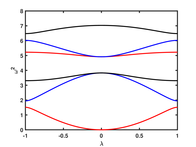
(a) Contract, $\sigma=-0.1$.

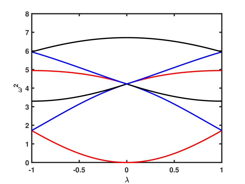
(b) $\sigma=0$.

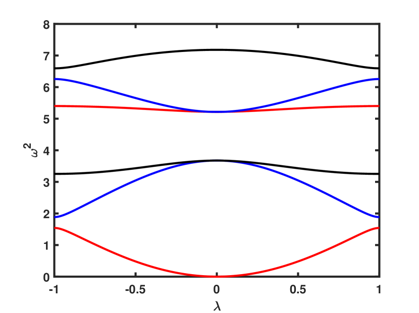
(c) Dilate, $\sigma=0.1$.

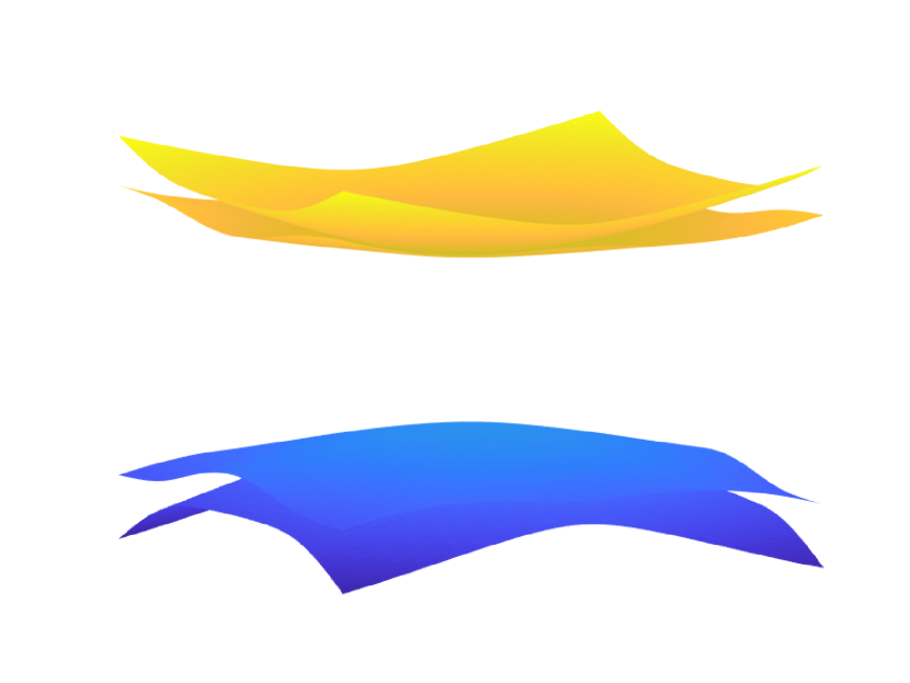
(d) Contract, $\sigma=-0.1$.

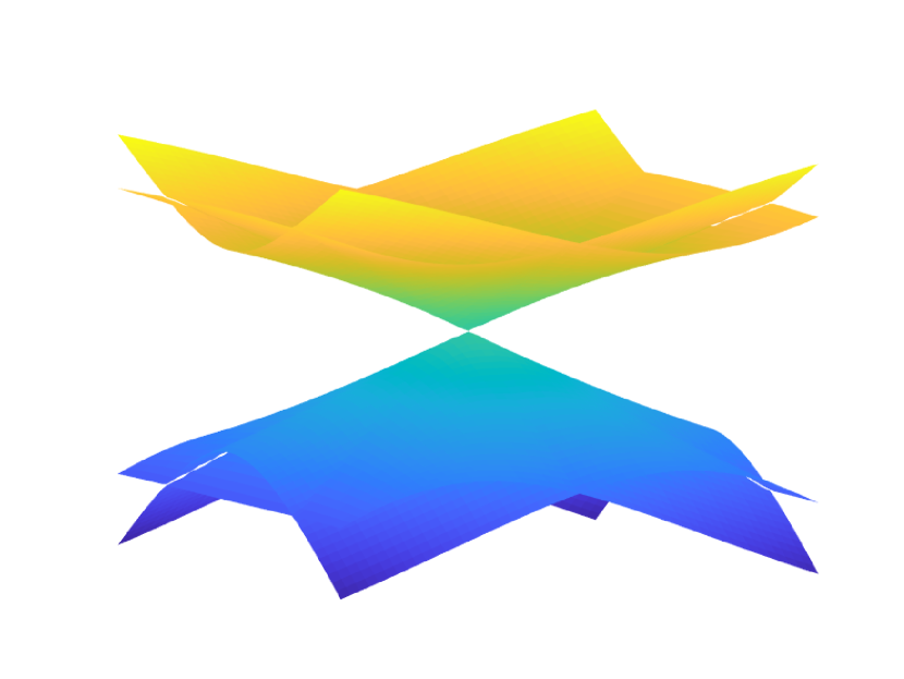
(e) $\sigma=0$.

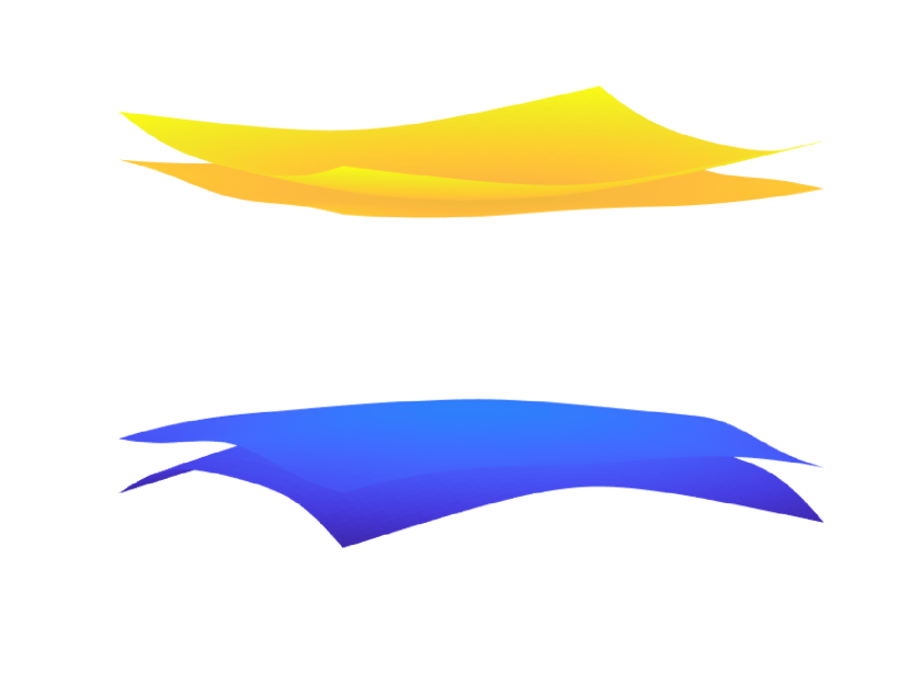
(f) Dilate, $\sigma=0.1$.

Figure 3: Top Panel: we plot the first six bands $\{\omega^{2}(\alpha)\}$ on the line segment $\overline{M_{1}M_{2}}$ in the dual unit cell. Bottom Panel: In these figures we plot the second to fifth dispersion surfaces $\{\omega^{2}(\alpha)\}$ near $\alpha=0$.

Then we plot the figures of how the dilation and contraction affect the band structure $\{\omega^{2}(\alpha,\sigma)\}_{\alpha\in Y^{\prime}}$ near $\alpha=0$. To be more specific, we consider the We let the inclusions be six circles centered at $\{P_{i,\sigma}\}_{i=1}^{6}$. We choose $\sigma=\mp 0.1$, corresponding to the contracted and dilated cases. Such examples are illustrated in Figure 2. In Figure 3(a), we plot the band structure $\{\omega^{2}(\alpha)\}_{\alpha\in Y^{\prime}}$ when the inclusions are contracted. We can see that the second and third bands detach from the fourth and fifth bands. This can be seen more clearly in Figure 3(d), where we plot the second to fifth band functions $\{\omega^{2}(\alpha,-0.1)\}_{\alpha\in Y^{\prime}}$ near the point $\alpha=0$. Similar separation also appears when the inclusions are dilated, see Figures 3(c) and 3(f). These results correspond to Section 3.3.

Finally, we compute the second to fifth eigenfunction of the original problem (5). And for simplicity we only discuss the contracted and dilated cases when $\sigma=\mp 0.1$. We first plot these figures in Figure 4.

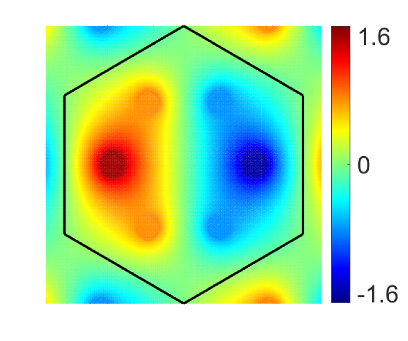
(a) Second, $\sigma=-0.1$

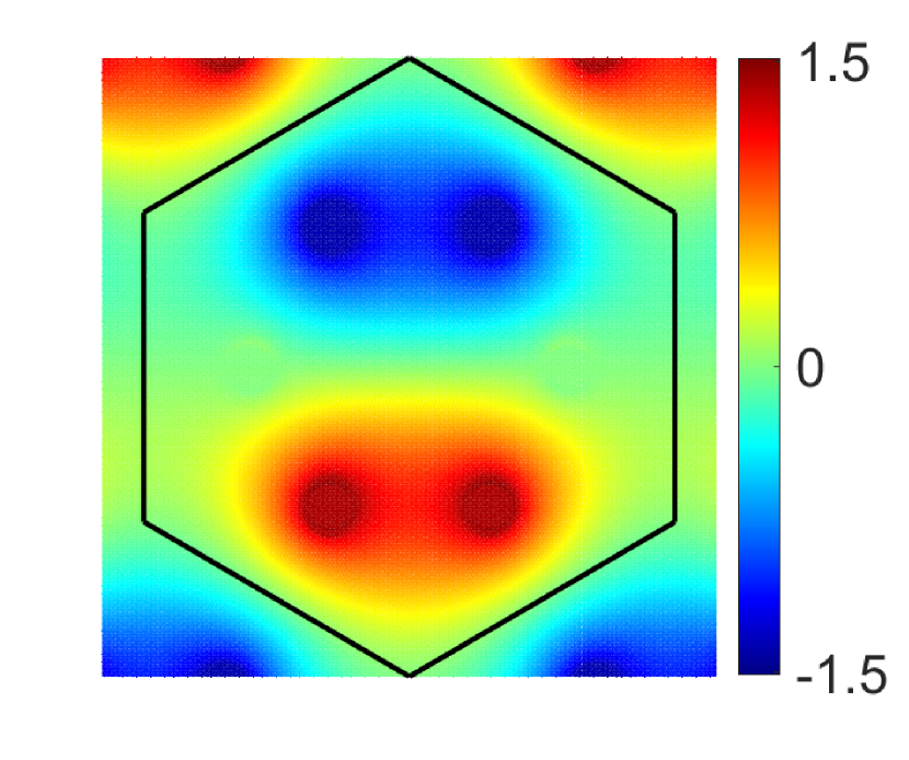
(b) Third, $\sigma=-0.1$

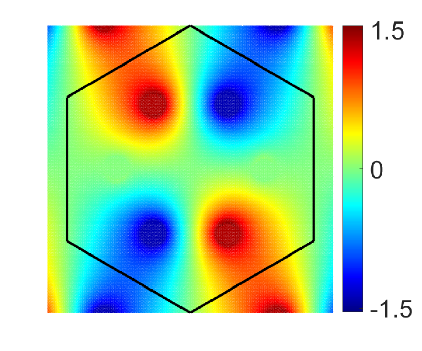
(c) Fourth, $\sigma=-0.1$

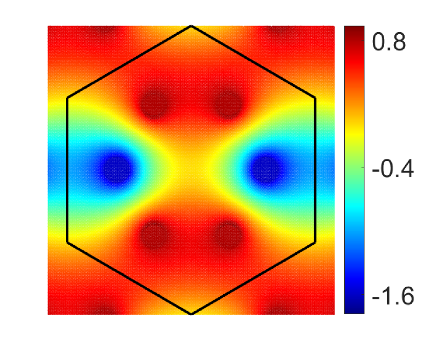
(d) Fifth, $\sigma=-0.1$

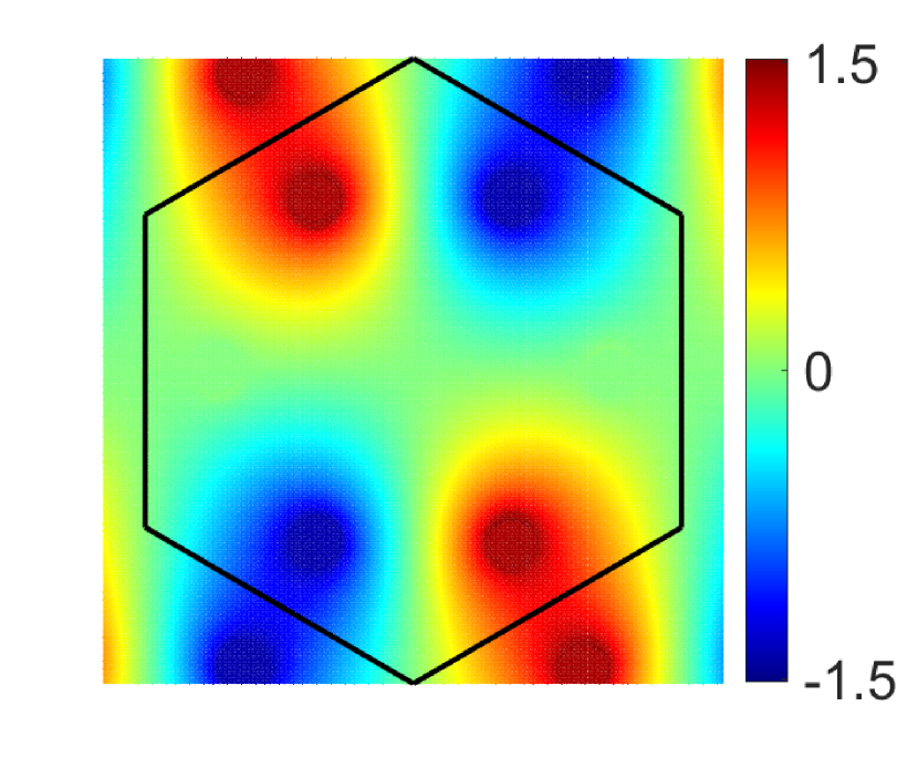
(e) Second, $\sigma=0.1$

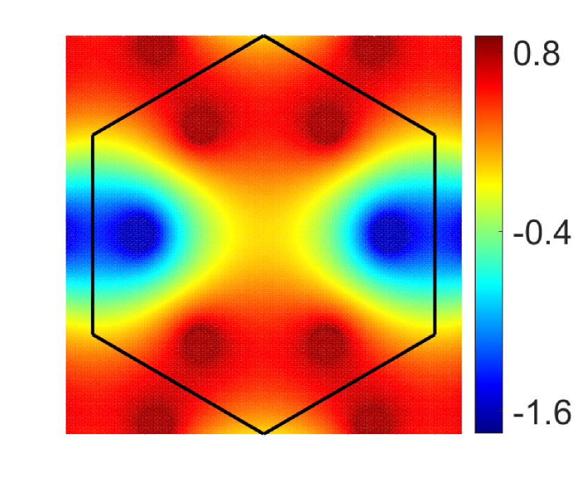
(f) Third, $\sigma=0.1$

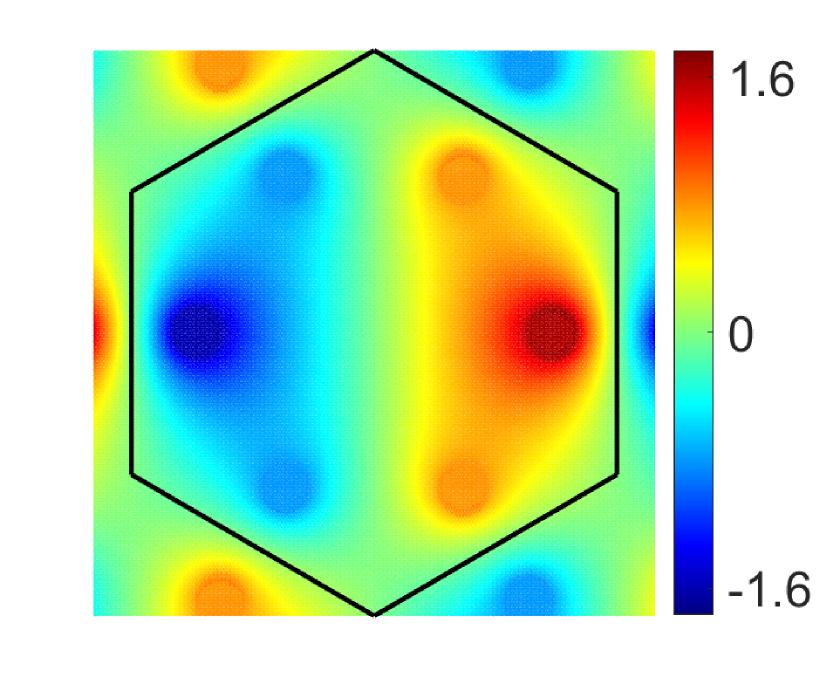
(g) Fourth, $\sigma=0.1$

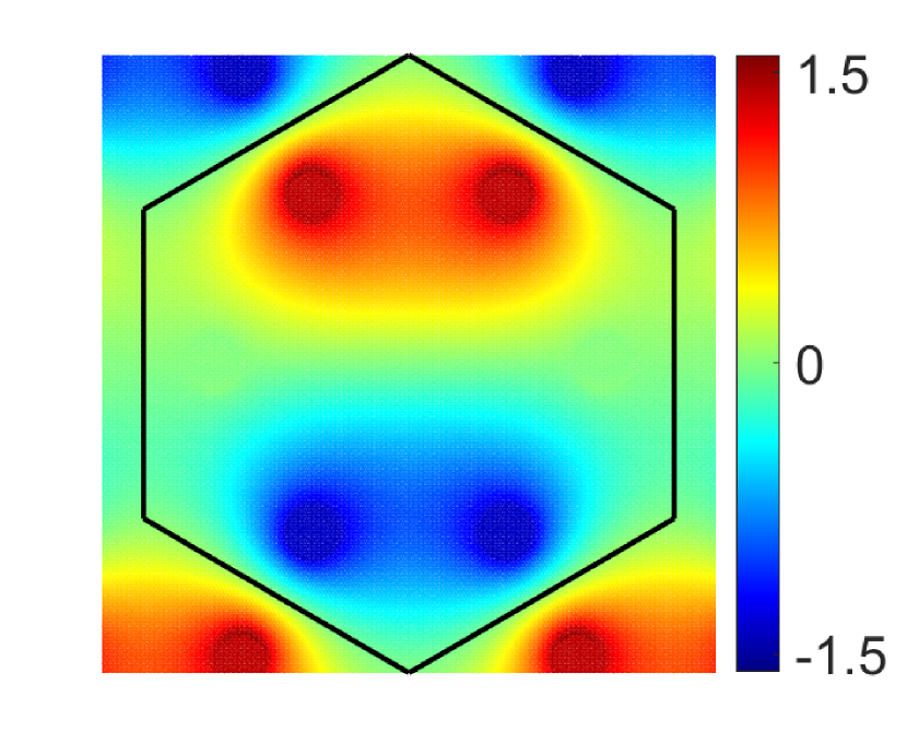
(h) Fifth, $\sigma=0.1$

Figure 4: In the top panel we plot the second to fifth eigenfunction when the inclusions are contracted. In the bottom panel we plot the second to fifth eigenfunction when the inclosions are dilated. By ’second’, ’third’, ’fourth’, ’fifth’ we mean the corresponding eigenfunction.

We can see from the figure that when the inclusions are contracted, the second and third eigenfunctions are inversion anti-symmetric with respect to the center $O$. When the inclusions are dilated, the second and third eigenfuntions are inversion symmetric with respect to the center $O$. We can conclude that there is a topological phase transition between the contracted and dilated case. This result also coincide with Section 4.2.

Appendix A Periodic Layer Potential and Their Properties

Here we define the double layer potential $\mathcal{D}^{0,0}_{D}$ for any $\varphi\in\mathbb{L}^{2}(\partial D)$:

(55) $$\textstyle\mathcal{D}_{D}^{0,0}[\varphi](x)\triangleq-\int_{\partial D}n_{y}\cdot\nabla G^{0,0}(x-y)\varphi(y)d\sigma(y),\quad x\in\mathbb{R}^{2}\backslash\partial D.$$

It satisfies the following jump relations [10]

(56) $$\textstyle\mathcal{D}^{0,0}_{D}[\varphi]\big{|}_{\pm}(y) =\textstyle\mp\frac{1}{2}\varphi(y)+\mathcal{K}^{0,0}_{D}[\varphi](y),$$

(57) $$\quad n_{y}\cdot\mathcal{D}_{D}^{0,0}[\varphi]\big{|}_{+}(y) \textstyle=n_{y}\cdot\nabla\mathcal{D}_{D}^{0,0}[\varphi]\big{|}_{-}(y).$$

And we list the mapping properties, whose proofs can be found in [31]

Lemma A.1 (Proposition 12.12, [31]).

The following equalities hold

(58) $$\textstyle\mathcal{K}_{D}^{0,0}[1]=\frac{1}{2}-\frac{|D|}{|Y|},\quad y\in\partial D,\qquad\mathcal{D}_{D}^{0,0}[1]=-\frac{|D|}{|Y|},\quad x\in Y\backslash D.$$

From this one can prove

Lemma A.2.

The operator $-\frac{1}{2}\operatorname{Id}+\mathcal{K}_{D}^{0,0}$, regarded as an operator from $\mathbb{L}^{2}(\partial D)$ to itself, has non-trivial kernel of 5 dimension. Further, for every $\psi\in\ker(-\frac{1}{2}\operatorname{Id}+\mathcal{K}_{D}^{0,0})$, it satisfies

$$\textstyle\psi=\sum_{j=1}^{6}c_{j}\chi_{{}_{\partial D_{j}}},\quad\sum_{j=1}^{6}c_{j}=0.$$

Proof A.3.

For any $\psi$ that satisfies $(-\frac{1}{2}\operatorname{Id}+\mathcal{K}_{D}^{0,0})[\psi]=0$, we have, by the jump relations (56), $\left.\mathcal{D}_{D}^{0,0}[\psi]\right|_{+}=0$ and $\mathcal{D}_{D}^{0,0}[\psi]$ is harmonic in $Y\backslash D$[31]. It immediately follows that, by the uniqueness of Dirichlet problem in $Y\backslash D$, $\mathcal{D}_{D}^{0,0}[\psi]\equiv 0$ for all $x\in Y\backslash D$.

By the jump relation (57) and the existence result, $\mathcal{D}_{D}^{0,0}[\psi]\equiv c_{j}$ on each inclusion $D_{j}$. So $\psi=c_{j}$ on $\partial D_{j}$ and for $x\in Y\backslash D$

$$\textstyle\mathcal{D}_{D}^{0,0}[\psi]=\mathcal{D}_{D}^{0,0}[\sum_{j=1}^{6}c_{j}\chi_{{}_{D_{j}}}]=-\sum_{j=1}^{6}\frac{|D|}{6|Y|}c_{j}=-\frac{|D|}{6|Y|}\sum_{j=1}^{6}c_{j}=0.$$

So $(c_{j})_{j=1}^{6}$, if regarded as a vector in $\mathbb{R}^{6}$, must satisfy $\sum_{j=1}^{6}c_{j}=0$. This fact means $\operatorname{dim}\ker(-\frac{1}{2}\operatorname{Id}+\mathcal{K}_{D}^{0,0})=5$.

Now we can state and prove the main proposition concerning $\ker[-\frac{1}{2}\operatorname{Id}+(\mathcal{K}_{D}^{0,0})^{\ast}]$: The kernel of the operator $-\frac{1}{2}\operatorname{Id}+(\mathcal{K}^{0,0}_{D})^{\ast}$ is five dimensional. Moreover, for any $\varphi\in\ker[-\frac{1}{2}\operatorname{Id}+(\mathcal{K}^{0,0}_{D})^{\ast}]$,

(59) $$\textstyle\mathcal{S}_{D}^{0,0}[\varphi]=\sum_{i=1}^{6}a_{i}\chi_{{}_{\partial D_{i}}},$$

where $\{a_{i}\}_{i=1}^{6}$ are real constants satisfying $\sum_{i=1}^{6}a_{i}=0.$

Proof A.4.

The first part is an immediate corollary from Lemma A.2, and noticing that

$$\textstyle\operatorname{dim}\ker\big{[}-\frac{1}{2}\operatorname{Id}+(\mathcal{K}_{D}^{0,0})^{\ast}\big{]}=\operatorname{dim}\ker\big{[}-\frac{1}{2}\operatorname{Id}+\mathcal{K}_{D}^{0,0}\big{]}.$$

Now suppose $\varphi_{j}\in\ker\big{[}-\frac{1}{2}\operatorname{Id}+(\mathcal{K}_{D}^{0,0})^{\ast}\big{]}$ for $j=1,2,\ldots,5$. We have, by definition and Lemma A.1:

$$\textstyle\frac{1}{2}\int_{\partial D}\varphi_{j}d\sigma(y)=\int_{\partial D}(\mathcal{K}^{0,0}_{D})^{\ast}[\varphi_{j}]d\sigma(y)=\int_{\partial D}\varphi_{j}\mathcal{K}_{D}^{0,0}[1]d\sigma(y)=(\frac{1}{2}-\frac{|D|}{|Y|})\int_{\partial D}\varphi_{j}d\sigma(y).$$

This implies $\varphi_{j}\in\mathbb{L}^{2}_{0}(\partial D)$. Thus, $\mathcal{S}_{D}^{0,0}[\varphi_{j}]$ is harmonic in $D$ and has homogeneous Neumann boundary on $\partial D$. By uniqueness result, $\mathcal{S}_{D}^{0,0}[\varphi_{j}]\equiv d_{jk}$ in $D_{k}$. If for all $j$, (59) holds, then we are done. Otherwise, suppose we have $\sum_{l=1}^{6}(d_{jl}-c_{j})=0,\quad j=1,2,\ldots,5.$ Since we can regard $(d_{jl})_{l=1}^{6}$ as vectors in $\mathbb{R}^{6}$. Obviously the vectors $\{(d_{jl})\}_{j=1}^{5}$ are linearly independent. And we argue by contradictory that the vectors $\{(d_{jl}-c_{j})\}_{j=1}^{5}$ are linearly independent for any real numbers $\{c_{j}\}_{j=1}^{5}$.

Suppose otherwise there exist $\{a_{j}\}_{j=1}^{5}$ that does not equals to zero at the same time, such that the following equality holds for some $\{c_{j}\}_{j=1}^{5}\subset\mathbb{R}$:

$$\textstyle\sum_{j=1}^{5}a_{j}(d_{jl})_{l=1}^{6}=\sum_{j=1}^{5}a_{j}c_{j}.$$

However, the above equality is equivalent to

$$\textstyle\sum_{j=1}^{5}\mathcal{S}^{0,0}_{D}[a_{j}\varphi_{j}](y)=\sum_{j=1}^{5}a_{j}c_{j},\quad y\in\partial D.$$

By Lemma 3.1, the sum $\sum_{j=1}^{5}a_{j}\varphi_{j}\equiv 0$, which is a contradictory.

Now we can assume, after a certain invertible linear transformation, there exist $\{\psi_{j}\}_{j=1}^{5}\subset\ker[-\frac{1}{2}\operatorname{Id}+(\mathcal{K}^{0,0})^{\ast}]$ and $\{d_{j}\}_{j=1}^{5}\subset\mathbb{R}$, such that

(60) $$[\mathcal{S}_{D}^{0,0}[\psi_{j}]+d_{j}]|_{D_{k}}=\mathrm{e}^{\mathrm{i}jk\pi/3},\quad j=1,2,\ldots 5.$$

We have, by definition

$$[\mathcal{S}^{0,0}_{D}[\psi_{j}](Ry)+d_{j}]|_{D_{k}}=\mathrm{e}^{\mathrm{i}j(k+1)\pi/3},\quad j=1,2,\ldots,5.$$

Multiplying the constant $\mathrm{e}^{\mathrm{i}j\pi/3}$ on both sides of (60), we have

$$[\mathcal{S}^{0,0}_{D}[\mathrm{e}^{\mathrm{i}j\pi/3}\psi_{j}](y)+d_{j}\mathrm{e}^{\mathrm{i}j\pi/3}]|_{D_{k}}=\mathrm{e}^{\mathrm{i}j(k+1)\pi/3},\quad j=1,2,\ldots,5.$$

Combining the above two equations, we have

(61) $$\mathcal{S}^{0,0}_{D}[\psi_{j}(Ry)-\mathrm{e}^{\mathrm{i}j\pi/3}\psi_{j}(y)]|_{D_{k}}=d_{j}(\mathrm{e}^{\mathrm{i}j\pi/3}-1),\quad j=1,2,\ldots,5.$$

By Lemma 3.1, we have $d_{j}=0$, and we have finished the proof of Appendix A.

Appendix B Representation of Solution

In this section we justify that the non-constant solution to the original problem (5) when $\omega=0$ can be represented by single layer potentials. From definition we have

(62) $$\textstyle\Delta G^{0,0}=\sum_{n\in\Lambda}\delta(x-n)-\frac{1}{|Y|}.$$

So when $x\in D$ we have by (62)

$$\textstyle u(x)-\frac{1}{|Y|}\int_{D} \textstyle u(z)dz=\int_{D}u(z)\Delta G^{0,0}(x-z)-\Delta u(z)G^{0,0}(x-z)dz$$

$$\textstyle=\int_{\partial D}n_{y}\cdot\nabla G(x-y)u|_{-}(y)-\left.n_{y}\cdot\nabla u(y)\right|_{-}G^{0,0}(x-y)d\sigma(y).$$

And we can obtain the following equality similarly

$$\textstyle-\frac{1}{|Y|}\int_{Y\backslash\overline{D}}u(z)dz =\textstyle\int_{Y\backslash\overline{D}}u(z)\Delta G^{0,0}(x-z)-\Delta u(z)G^{0,0}(x-z)dz$$

$$\textstyle=\int_{\partial D}-n_{y}\cdot\nabla G(x-y)u|_{+}(y)+\left.n_{y}\cdot\nabla u(y)\right|_{+}G^{0,0}(x-y)d\sigma(y).$$

Combining the above two equalities and the jump condition in (5), we have

(65) $$\textstyle u(x)-\frac{1}{|Y|}\int_{Y}u(z)dz=\mathcal{S}^{0,0}_{D}[\left.n_{y}\cdot\nabla u(y)\right|_{+}-\left.n_{y}\cdot\nabla u(y)\right|_{-}](x).$$

Here we notice that the constant solution cannot be represented by single layer potential.

References

• [1] M. J. Ablowitz, C. W. Curtis, and Y. Zhu, On tight-binding approximations in optical lattices, Stud. Appl. Math., 129 (2012), pp. 362–388.
• [2] M. J. Ablowitz, S. D. Nixon, and Y. Zhu, Conical diffraction in honeycomb lattices, Phys. Rev. A, 79 (2009), p. 053830.
• [3] H. Ammari and J. Cao, Unidirectional edge modes in time-modulated metamaterials, Proc. A., 478 (2022).
• [4] H. Ammari and B. Davies, A fully coupled subwavelength resonance approach to filtering auditory signals, Proc. A., 475 (2019), p. 20190049.
• [5] H. Ammari, B. Davies, E. O. Hiltunen, H. Lee, and S. Yu, Bound states in the continuum and Fano resonances in subwavelength resonator arrays, J. Math. Phys., 62 (2021), p. 101506.
• [6] H. Ammari, B. Davies, E. O. Hiltunen, H. Lee, and S. Yu, Exceptional points in parity–time-symmetric subwavelength metamaterials, SIAM J. Math. Anal., 54 (2022), pp. 6223–6253.
• [7] H. Ammari, B. Davies, E. O. Hiltunen, and S. Yu, Topologically protected edge modes in one-dimensional chains of subwavelength resonators, J. Math. Pures Appl., 144 (2020), pp. 17–49.
• [8] H. Ammari, B. Fitzpatrick, D. Gontier, H. Lee, and H. Zhang, Minnaert resonances for acoustic waves in bubbly media, Ann. Inst. H. Poincaré Anal. Non Linéaire, 35 (2018), pp. 1975–1998.
• [9] H. Ammari, B. Fitzpatrick, E. O. Hiltunen, H. Lee, and S. Yu, Honeycomb-lattice Minnaert bubbles, SIAM J. Math. Anal., 52 (2020), pp. 5441–5466.
• [10] H. Ammari, B. Fitzpatrick, H. Kang, M. Ruiz, S. Yu, and H. Zhang, Mathematical and Computational Methods in Photonics and Phononics, American Mathematical Society, 2018.
• [11] H. Ammari, B. Fitzpatrick, H. Lee, S. Yu, and H. Zhang, Subwavelength phononic bandgap opening in bubbly media, J. Differential Equations, 263 (2017), pp. 5610–5629.
• [12] H. Ammari, H. Kang, and H. Lee, Layer Potential Techniques in Spectral Analysis, vol. 153 of Mathematical Surveys and Monographs, American Mathematical Society, Providence, RI, 2009.
• [13] Y. Cao and Y. Zhu, Double conical degeneracy on the band structure of periodic Schrödinger operators, (2022), https://arxiv.org/abs/2212.05210.
• [14] M. Cassier and M. I. Weinstein, High contrast elliptic operators in honeycomb structures, Multiscale Model. Simul., 19 (2021), pp. 1784–1856.
• [15] C. L. Fefferman, J. P. Lee-Thorp, and M. I. Weinstein, Edge states in honeycomb structures, Ann. PDE, 2 (2016).
• [16] C. L. Fefferman, J. P. Lee-Thorp, and M. I. Weinstein, Honeycomb Schrödinger operators in the strong binding regime, Commun. Pure Appl. Math., 71 (2017), pp. 1178–1270.
• [17] C. L. Fefferman and M. I. Weinstein, Honeycomb lattice potentials and Dirac points, J. Amer. Math. Soc., 25 (2012), pp. 1169–1220.
• [18] C. L. Fefferman and M. I. Weinstein, Wave packets in honeycomb structures and two-dimensional dirac equations, Comm. Math. Phys., 326 (2013), pp. 251–286.
• [19] C. L. Fefferman and M. I. Weinstein, Continuum Schroedinger operators for sharply terminated graphene-like structures, Comm. Math. Phys., 380 (2020), pp. 853–945.
• [20] H. Guo, X. Yang, and Y. Zhu, Unfitted Nitsche’s method for computing band structures of phononic crystals with periodic inclusions, Comput. Methods Appl. Mech. Eng., 380 (2021), p. 113743.
• [21] H. Guo, X. Yang, and Y. Zhu, Unfitted Nitsche’s method for computing wave modes in topological materials, J. Sci. Comput., 88 (2021).
• [22] H. Guo, M. Zhang, and Y. Zhu, ThreeFold weyl points for the Schrödinger operator with periodic potentials, SIAM J. Math. Anal., 54 (2022), pp. 3654–3695.
• [23] F. D. M. Haldane and S. Raghu, Possible realization of directional optical waveguides in photonic crystals with broken time-reversal symmetry, Phys. Rev. Lett., 100 (2008), p. 013904.
• [24] M. Z. Hasan and C. L. Kane, Colloquium: Topological insulators, Rev. Mod. Phys., 82 (2010), pp. 3045–3067.
• [25] C.-H. Hsu, Z.-Q. Huang, C. P. Crisostomo, L.-Z. Yao, F.-C. Chuang, Y.-T. Liu, B. Wang, C.-H. Hsu, C.-C. Lee, H. Lin, and A. Bansil, Two-dimensional topological crystalline insulator phase in sb/bi planar honeycomb with tunable dirac gap, Sci. Rep., 6 (2016).
• [26] Z. Lan, M. L. Chen, F. Gao, S. Zhang, and W. E. Sha, A brief review of topological photonics in one, two, and three dimensions, Rev. Phys., 9 (2022), p. 100076.
• [27] J. P. Lee-Thorp, M. I. Weinstein, and Y. Zhu, Elliptic operators with honeycomb symmetry: Dirac points, edge states and applications to photonic graphene, Arch. Ration. Mech. Anal., 232 (2018), pp. 1–63.
• [28] A. H. C. Neto, F. Guinea, N. M. R. Peres, K. S. Novoselov, and A. K. Geim, The electronic properties of graphene, Rev. Mod. Phys., 81 (2009), pp. 109–162.
• [29] T. Ozawa, H. M. Price, A. Amo, N. Goldman, M. Hafezi, L. Lu, M. C. Rechtsman, D. Schuster, J. Simon, O. Zilberberg, and I. Carusotto, Topological photonics, Rev. Mod. Phys., 91 (2019), p. 015006.
• [30] X.-L. Qi and S.-C. Zhang, Topological insulators and superconductors, Rev. Mod. Phys., 83 (2011), pp. 1057–1110.
• [31] M. D. Riva, M. L. de Cristoforis, and P. Musolino, Singularly Perturbed Boundary Value Problems, Springer International Publishing, 2021.
• [32] P. R. Wallace, The band theory of graphite, Phys. Rev., 71 (1947), pp. 622–634.
• [33] L.-H. Wu and X. Hu, Scheme for achieving a topological photonic crystal by using dielectric material, Phys. Rev. Lett., 114 (2015), p. 223901.
• [34] Y. Yang, Y. F. Xu, T. Xu, H.-X. Wang, J.-H. Jiang, X. Hu, and Z. Hang, Visualization of a unidirectional electromagnetic waveguide using topological photonic crystals made of dielectric materials, Phys. Rev. Lett., 120 (2018), p. 217401.
• [35] S. Yves, R. Fleury, T. Berthelot, M. Fink, F. Lemoult, and G. Lerosey, Crystalline metamaterials for topological properties at subwavelength scales, Nat. Commun., 8 (2017).