Feature Map for Quantum Data: Probabilistic Manipulation

Abstract

The kernel trick in supervised learning signifies transformations of an inner product by a feature map, which then restructures training data in a larger Hilbert space according to an endowed inner product. A quantum feature map corresponds to an instance with a Hilbert space of quantum states by fueling quantum resources to ML algorithms. In this work, we point out that the quantum state space is specific such that a measurement postulate characterizes an inner product and that manipulation of quantum states prepared from classical data cannot enhance the distinguishability of data points. We present a feature map for quantum data as a probabilistic manipulation of quantum states to improve supervised learning algorithms.

In supervised learning, one aims to construct a model that makes predictions based on training data. Recently, the framework has begun to apply the laws of quantum mechanics, Quantum Machine Learning, to fuel nonclassical properties such as entanglement and superposition to machine learning (ML) algorithms for further advantages, see e.g., Biamonte et al. (2017); Maria Schuld (2018); Dunjko et al. (2016). One way to apply Quantum Information Theory (QIT) in ML is to process ML algorithms with quantum states prepared according to classical data.

From the view of QIT, the state preparation rephrases embedding classical data to quantum systems. Technically, the space of quantum states is described by a Hilbert space where the measurement postulate, called the Born rule, specifies an inner product von Neumann (1932). From the view of ML, embedding data in a Hilbert space corresponds to a feature map: its quantum application is called a quantum feature map Schuld and Killoran (2019); Schuld (2021). Then, the resulting quantum states and the Hilbert space are referred to as feature vectors and a feature space, respectively.

On the one hand, a quantum feature map allows one to exploit quantum resources such as entanglement and superposition existing in quantum states to enhance ML algorithms. As a result, one may envisage quantum advantages over classical counterparts. On the other hand, one notices that the quantum state space is a specific and restricted object. It is a Hilbert space entirely characterized by the postulates of quantum theory von Neumann (1932).

The consequences show that once a feature map prepares quantum states, quantum operations are contractive, i.e., the norm of feature vectors does not increase Pérez-García et al. (2006). Moreover, a mathematical space describing quantum states is not hypothetical: the measurement postulate defines an inner product uniquely in the space, known as the Gleason theorem Gleason (1957). The uniqueness implies limitations on the so-called kernel tricks in the quantum feature space. Apart from the fact the quantum state preparation corresponds to a feature map per se, little is known about how quantum principles can be incorporated to feature vectors to enhance ML algorithms.

In this work, we show that once quantum states are prepared for an ML algorithm, their distinguishability does not increase by a feature map. In contrast to classical ML algorithms, quantum data cannot be manipulated such that their distinguishability is enhanced. We then present a general manipulation of quantum data, namely a feature map for quantum data, by relaxing the trace-preserving condition, as a versatile tool to improve ML algorithms. We also develop a circuit construction of a feature map for quantum data and demonstrate its advantages in supervised learning for binary classification.

We first summarize a feature map as a general process of embedding data into a larger Hilbert space. For sample data $D=\{x_{m}\in\mathbbm{R}^{N}\}$, a feature map $\phi:\mathbbm{R}^{N}\rightarrow\mathcal{H}$ for $\dim(\mathcal{H})\geq N$ induces an inner product, $\kappa(x_{m},x_{n})=\langle{\phi}(x_{m}),{\phi}(x_{n})\rangle_{\mathcal{H}}$ on a resulting Hilbert space, where $\kappa:(x_{m},x_{n})\mapsto\mathbbm{R}$ denotes a kernel function via an inner product on the feature space $\mathcal{H}$. Thus, a structure is introduced to data in terms of an inner product.

A quantum feature space is a Hilbert space of quantum states such that $n$ qubits define a $2^{n}$-dimensional space on which a quantum state could contain superposition or entanglement. A quantum feature map devises a quantum circuit $U_{\phi}$ that prepares states from sample data as follows,

$$\phi~{}:~{}x_{m}\in\mathbb{R}^{N}\mapsto\rho_{\phi}(x_{m})\in S(\mathcal{H})$$ (1)

where $\rho_{\phi}(x_{m})$ is a quantum state on a Hilbert space $\mathcal{H}$ and $S(\mathcal{H})$ denotes the set of states. Consequently, a kernel is a mapping from a pair of datapoints to an inner product in the feature space via a feature map,

$$\kappa(x_{m},x_{n})=\mathrm{tr}[\rho_{\phi}(x_{m})\rho_{\phi}(x_{n})]~{}~{}$$ (2)

which is in fact given by the measurement postulate. For instance, Eq. (2) may be obtained as a probability of obtaining an outcome on positive-operator-valued-measure $\alpha\rho_{\phi}(x_{n})$ with some $\alpha>0$ for a state $\rho_{\phi}(x_{m})$. Or, it corresponds to the estimation of the visibility of two states in an interferometric setup, e.g., the Hong-Ou-Mandel fringe for photonic qubits Hong et al. (1987); Horodecki and Ekert (2002).

The Hilbert space of quantum systems is specific in the sense that an inner product is introduced by a measurement postulate Gleason (1957); von Neumann (1932). It immediately implies limitations of a quantum feature map in that, contrasting to feature spaces by classical systems, quantum data cannot be repeatedly embedded in some other feature space such that they are structured with a higher distinguishability.

Proposition. Quantum data cannot be embedded in a feature space with enhanced distinguishability.

Proof. We first consider cases that mapping quantum data directly back to a classical feature space by measurements. It is clear that non-orthogonal states cannot be perfectly distinguished, and thus the mapping introduces either an error Helstrom (1969) or ambiguous outcomes Ivanovic (1987); Dieks (1988); Peres (1988), see also Bergou (2007); Bae and Kwek (2015). There are fundamental limitations in the bounds Croke et al. (2008); Bae et al. (2011); Hwang and Bae (2010)

Or, one can consider a feature map for quantum data as embedding quantum data to high-dimensional quantum systems and then a measurement. A quantum channel, denoted by $\Lambda:\mathcal{H}\rightarrow\widetilde{H}$ for $\mathrm{dim}\mathcal{H}\leq\mathrm{dim}\widetilde{\mathcal{H}}$, corresponds to a positive and completely positive map for quantum states. Such a map does not increase pairwise distinguishability: for two states $\rho_{1}$ and $\rho_{2}$ appearing with probabilities $q_{1}$ and $q_{2}$, it holds that

$$\|\Lambda[X]\|_{1}\leq\|X\|_{1},~{}\mathrm{for}~{}X=q_{1}\rho_{1}-q_{2}\rho_{2}\ngeq 0$$ (3)

where $\|\cdot\|_{1}$ denotes the $L_{1}$ norm, i.e., $\|A\|_{1}=\mathrm{tr}\sqrt{A^{\dagger}A}$. $\Box$

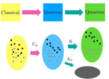
Figure 1: A quantum feature map transforms classical data (yellow) to quantum states (blue), where the mathematical structure is provided by a Hilbert space where an inner product is realized by a measurement axiom. A feature map defined by Kraus operators ($K,K_{0}$) for quantum states introduces two ensembles. One is by $K$ in which states are manipulated beyond the contractive properties (green), i.e., states can be even better distinguished. The other Kraus operator $K_{0}$ collects states whenever $K$ is unsuccessful.

In the above, one can consider other measures of distinguishability such as von Neumann entropy or min-entropy and find the same conclusion Jozsa and Schlienz (2000); Bae (2013).

We put a step forward to relaxing quantum channels to quantum filtering operations and present a general form of a feature map for quantum data to enhance ML algorithms with quantum states. To this end, we recall that a quantum channel can be described as a dynamics of a subsystem that interacts with an ancilla through a unitary transformation. When a state and an ancilla initialized in $\rho_{S}\otimes|a\rangle_{A}\langle a|$ result in $U_{SA}\rho_{S}\otimes|a\rangle_{A}\langle a|U_{SA}^{\dagger}$ for some interaction $U_{SA}$, a measurement on an ancilla in an orthonormal basis $\{|i\rangle_{A}\}$ finds the probability of having an outcome $i$,

$$p_{A}(i)=\mathrm{tr}[U_{SA}\rho_{S}\otimes|a\rangle_{A}\langle a|U_{SA}^{\dagger}|i\rangle_{A}\langle i|].$$

Then, the resulting state of a system can be described by

$$\rho_{S}(i)=\frac{1}{p_{A}(i)}{K_{i}}\rho K_{i}^{\dagger}~{}~{}\mathrm{where}~{}K_{i}=_{A}\langle i|U_{SA}|a\rangle_{A}$$ (4)

where $\{K_{i}\}$ are called Kraus operators, satisfying the relation $\sum_{i}K_{i}^{\dagger}K_{i}=\mathbbm{I}$.

It is worth mentioning that probabilistic manipulations of quantum states by exploiting Kraus operators have been used to resolve non-trivial problems in various contexts of quantum information applications. In entanglement theory, two-qubit entangled states can be transformed to a more entangled one with some probability by local operations and classical operations, called local filtering Verstraete et al. (2001); Verstraete and Wolf (2002). The protocol for distilling entanglement can be rephrased as a sequence of local filtering operations Bennett et al. (1996); Deutsch et al. (1996). In fact, local filtering operations can also reveal hidden nonlocality existing in some entangled states Popescu (1995). In experiments, a post-selection technique can be described by Kraus operators. For instance, one way to demonstrate a quantum gate with photonic qubits which hardly interact with each other is to select particular measurement outcomes whenever photon-photon interactions were successful, see e.g., Lim et al. (2011).

We now present a feature map for quantum data via Kraus operators as a probabilistic strategy of manipulating quantum states to enhance ML algorithms, see Fig. 1. Let $K$ and $K_{0}$ denote two Kraus operators such that $K$ describes a desired transformation of quantum data and $K_{0}=(\mathbb{I}-K^{\dagger}K)^{1/2}$ otherwise. Then, quantum data previously prepared by a quantum feature map $\phi$ denoted by $D_{\phi}=\{\rho_{\phi}(x_{m})\in S(\mathcal{H})\}$ can be transformed to $\widetilde{D}_{\phi}=\{\widetilde{\rho}_{\phi}(x_{m})\in S(\widetilde{\mathcal{H}})\}$ such that

$$K~{}:~{}{\rho}_{\phi}(x_{m})\mapsto\widetilde{\rho}_{\phi}(x_{m})~{}\mathrm{where}~{}$$ (5)

$$\widetilde{\rho}_{\phi}(x_{m})=\frac{K\rho_{\phi}(x_{m})K^{\dagger}}{p(x_{m})}~{}\mathrm{with}~{}p(x_{m})=\mathrm{tr}[K^{\dagger}K\rho_{\phi}(x_{m})].$$

From Proposition, we can safely restrict the consideration to the case $\dim(\widetilde{\mathcal{H}})=\dim({\mathcal{H}})$ due to no advantage of utilizing a larger Hilbert space of quantum states. It is straightforward to see that, once the transformation is successful, a Kraus operator also leads to a kernel:

$$\kappa(\rho_{\phi}(x_{m}),\rho_{\phi}(x_{n}))=\mathrm{tr}[\widetilde{\rho}_{\phi}(x_{m})\widetilde{\rho}_{\phi}(x_{n})]$$ (6)

Therefore, the task to enhance ML algorithms for quantum data is to identify a Kraus operator $K$ for manipulating quantum sample data beyond unitary transformations. If no enhancement occurs, one returns a trivial choice $K=\mathbbm{I}$.

One may assert the weakness that a feature map in Eq. (5) is probabilistic so that for a large number of datapoints, the probability of its realization $p(x_{1})\times p(x_{2})\times\cdots\times p(x_{m})\times\cdots$ quickly falls to zero. A collective interaction over blocks of quantum data can offer a prescription. That is, a Kraus operator is constructed for quantum states $D_{\phi}=\{\rho_{\phi}(x_{m})\in S(\mathcal{H})\}$,

$$K:\bigotimes_{m}{\rho}_{\phi}(x_{m})\mapsto\bigotimes_{m}\widetilde{\rho}_{\phi}(x_{m})$$ (7)

that prevents the overall success probability from dropping out to zero. Note that the success probability is given by $p(x_{1},\cdots,x_{m})=\mathrm{tr}[K^{\dagger}K\bigotimes_{m}{\rho}_{\phi}(x_{m})]$, which could be low but does not depend on the size of data. Thus, the price to pay for a non-vanishing probability is to build a Kraus operator $K$ for interaction among all datapoints, see $V(\theta)$ in Fig. 2.

In the following, we revisit supervised learning for binary classification: a training dataset is given as follows,

$$D=\{(x_{1},y_{1}),\dots,(x_{M},y_{M}):x_{m}\in\mathbbm{R}^{N},~{}y_{m}=\pm 1\}.$$ (8)

A linear hyperplane is sought to separate the set ${D}$ into two, one with $y_{m}=+1$ and the other with $y_{m}=-1$. A kernelized support vector machine applies a kernel $\phi:\mathbbm{R}^{N}\rightarrow\mathbbm{R}^{L}$ for $L\geq N$ so that the decision boundary can be characterized in a higher-dimensional Hilbert space by a normal vector $w\in\mathbbm{R}^{L}$ such that $f(x)=w^{\top}\phi(x)$. A decision function is given as the sign of $f(x)$. The classification function can be obtained as,

$$f(x)=\sum_{m}y_{m}\kappa(x_{m},x)$$ (9)

where uniform weights are assumed and the kernel $\kappa$ depends on the choice of a feature map $\phi$.

For simplicity, let us consider an amplitude encoding as a quantum feature map that prepares quantum states from sample data $D$,

$$\rho_{\phi}(x_{m})=|\psi_{x_{m}}\rangle\langle\psi_{x_{m}}|~{}\mathrm{where}~{}|\psi_{x_{m}}\rangle=\sum_{i=0}^{N-1}x_{m,i}|i\rangle.$$ (10)

To apply a SWAP-test based classifier Schuld et al. (2017), we write by $U$ a quantum circuit for the state preparation,

$$U|0\rangle^{\otimes l}=\frac{1}{\sqrt{M}}\sum_{m=1}^{M}|m\rangle_{L}|\psi_{x_{m}}\rangle_{T}|\psi_{x}\rangle_{t}|0\rangle_{S}|s_{m}\rangle_{C},~{}~{}~{}$$ (11)

where $l=(2+\log M+2\log N)$, see also Fig. 2. The first register (L) labels input data, the second one (T) collects training quantum data, the third one (t) contains a test state, the fourth one (S) is an ancilla needed for a SWAP test, and the last one (C) denotes a binary classification of training data: $|s_{m}\rangle=|0\rangle$ for $y_{m}=-1$ and $|s_{m}\rangle=|1\rangle$ for $y_{m}=1$. Registers (S) and (C) contain single qubits.

Figure 2: (A) A quantum feature map $U$ prepares quantum states from data, see the main text. (B) A feature map for quantum data implements a probabilistic transformation on both training and test data, i.e., when an outcome $0$ only is obtained in the register $F$. An interaction $V(\theta)$ may be trained to build an efficient feature map. (C) A Hadamard classifier is implemented with a SWAP test.

Then, a Hadamard classifier, see the dotted box (C) in Fig. 2, applies a SWAP test for states in registers $T$ and $t$. Qubits in registers in $S$ and $C$ are measured in the computational basis $\{|0\rangle_{z},|1\rangle_{z}\}$, respectively. The classifier in Eq. (9) can be constructed from outcomes in the registers. When an outcome $0$ $(1)$ is obtained in register $C$, states in registers $T$ are given by $\rho$ $(\sigma)$ where

$$\rho = \frac{1}{M_{A}}\sum_{y_{m}=-1}\rho_{\phi}(x_{m})~{}\mathrm{and}~{}\sigma=\frac{1}{M_{B}}\sum_{y_{m}=1}\rho_{\phi}(x_{m}),~{}~{}~{}$$ (12)

where $M_{A}=|\{x_{m}:y_{m}=-1\}|$ and $M_{B}=|\{x_{m}:y_{m}=1\}|$. Given an outcome $0$ in register $C$, a measurement is performed in register $S$: probabilities of $0$ and $1$ are given by $(1\pm\langle\psi_{x}|\rho|\psi_{x}\rangle)/2$, respectively. When an outcome in register $C$ is $1$, probabilities of $0$ and $1$ in register $S$ are given by $(1\pm\langle\psi_{x}|\sigma|\psi_{x}\rangle)/2$. Hence, from the probabilities, one can find the classification function in Eq. (9) as

$$f(x)=\langle\psi_{x}|\rho-\sigma|\psi_{x}\rangle$$ (13)

The empirical risk with the loss function by $L(f(x),y)=yf(x)$ is given by

$$R_{L} = \frac{1}{M}\sum_{m}L(f(x_{m}),y_{m})=-\mathrm{tr}[(\rho-\sigma)^{2}],$$ (14)

which also quantifies a classifier. Hence, a quantum feature map that maximizes the Hilbert-Schmidt distance between two ensembles $\rho$ and $\sigma$ builds a classifier with the least empirical risk Lloyd et al. (2021).

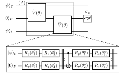
Figure 3: An interaction that realizes a feature map for quantum data, see Fig. 2, is designed as $V_{TFt}(\theta)=\widetilde{V}_{Ft}(\theta)\widetilde{V}_{TF}(\theta)$ and trained. A parameterized quantum circuit $\widetilde{V}(\theta)$ is chosen such that it contains arbitrary single qubit rotations and controlled-NOT gates.

A feature map in Eq. (7) applies to quantum data in Eq. (11) to enhance quantum supervised learning for binary classification. The map is facilitated by a unitary transformation $V(\theta)$ over training and test data as well as an ancilla $F$,

$$V(\theta)\sum_{m=1}^{M}|\psi_{x_{m}}\rangle_{T}|\psi_{x}\rangle_{t}|0\rangle_{F}=$$

$$\sum_{m=1}^{M}K(\theta)|\psi_{x_{m}}\rangle_{T}|\psi_{x}\rangle_{t}|0\rangle_{F}+\sum_{m=1}^{M}K_{0}(\theta)|\psi_{x_{m}}\rangle_{T}|\psi_{x}\rangle_{t}|1\rangle_{F}.~{}~{}~{}$$

An interaction $V(\theta)$ is to be trained to minimize the empirical risk in Eq. (14). Once a desired one $K(\theta)$ is realized with an ancilla state $|0\rangle_{F}$, ensembles of training data are transformed, denoted by $\widetilde{\rho}$ and $\widetilde{\sigma}$, respectively, similarly to ensembles in Eq. (12), and the classifier is given by, ${f}(x)=\langle\widetilde{\psi}_{x}|\widetilde{\rho}-\widetilde{\sigma}|\widetilde{\psi}_{x}\rangle$. Resulting quantum data with $|1\rangle_{F}$ that is not of interest will be discarded. In practice, an efficient unitary $V(\theta)$ may be designed as a parameterized quantum circuit and trained to minimize the cost function ${C}(\theta)={R}_{L}({f}_{\mathrm{}})$, as it is shown in Fig. 3. If a feature map by a Kraus operator $K(\theta)$ cannot make any advantage, an optimal parameter after training would return $V(\theta)=\mathbbm{I}$.

Let us illustrate the usefulness of a feature map for quantum data, for instance, the Iris dataset and the modified national institute of standard and technology (MNIST) dataset. In the former, Iris versicolor and Iris setosa are set as class $A$ and $B$, respectively. Then, sepal lengths and sepal widths are given as input data. We pick the $36$-th data in the Iris versicolor and the $34$-th data in the Iris setosa as the training dataset, and the $29$-th data in the Iris versicolor for the test one,

$$\mathrm{Training~{}data}~{} : \{((0,1),-1),((0.796,0.607),1)\},$$

$$\mathrm{Test~{}data} : ((-0.557,0.83),-1)$$

For the latter, we consider the images of $3$ and $6$ for binary classification. For convenience, we rescale each image from $28\times 28$ pixels to $4\times 4$ pixels Farhi and Neven (2018). In both cases, we use a classical optimizer COBYLA to train the parameters.

	Iris Dataset		MNIST Dataset
	$V(\theta)=\mathbbm{I}$	$V(\theta)\neq\mathbbm{I}$	$V(\theta)=\mathbbm{I}$	$V(\theta)\neq\mathbbm{I}$
Empirical Risk	$-1.251$	$-2.666$	$-1.534$	$-1.963$
Classifier	$-0.708$	$-0.996$	$0.121$	$0.056$
Probability	$-$	$0.475$	$-$	$0.647$
Decision	$-1$	$-1$	$1$	$1$

Table 1: A feature map for quantum data, denoted by $V(\theta)$, see Fig. 3, is trained for binary classification with datasets from Iris and MNIST. The case that a feature is not applied to quantum data is denoted by $V(\theta)=\mathbbm{I}$. The figure of merit is the empirical risk in Eq. (14), which is smaller whenever $V(\theta)$ is trained for both datasets. The success probabilities are maintained as $0.457$ and $0.647$.

Finally, we reiterate that a feature map for quantum data presents a strategy for enhancing an ML algorithm for quantum states prepared according to a quantum feature map. It could be compared with the quantum embedding of classical data shown in Ref. Lloyd et al. (2021), which formulates training the state preparation to improve ML algorithms with quantum states. It is worth mentioning that, with some probability, our results always improve a quantum feature map or the quantum embedding, since a unitary transformation is an instance of a Kraus operator. Further enhancements of an ML algorithm may be envisaged by combining both strategies, i.e., with optimal embedding followed by filtering operations: in Fig. 2 both $U$ and $V(\theta)$ are trained. Hence, a feature map for quantum data is a versatile tool to enhance existing ML algorithms.

In conclusion, we have established a general framework for manipulating quantum data and then shown its applications to an ML algorithm for binary classification. We have also developed a circuit construction for a feature map for quantum data. In particular, our results shed light on the opportunity of restructuring quantum data on a Hilbert space beyond the constraint of contractivity. With some probability, quantum states can be distributed in a quantum feature space such that they are better distinguishable. We have applied the results to supervised learning for binary classification and demonstrated enhancements in the empirical risk. Our results present a versatile tool readily applicable to improve existing quantum ML algorithms.

I Acknowledgement

This work is supported by National Research Foundation of Korea (NRF-2019M3E4A1080001) and the ITRC (Information Technology Research Center) Program (IITP-2022-2018-0-01402).

II Appendix : MNIST data

The MNIST dataset contains pixelized $28\times 28$ hand-writting images of numbers from $0$ to $9$. We rescale the $28\times 28$ images to $4\times 4$ to encode input data into quantum states Farhi and Neven (2018). A pixel data with a value $0$ to $255$ are normalized such that they are mapped to amplitudes of a quantum state. We pick numbers $3$ and $6$. Then, the training dataset

$$\mathcal{D}=\{(x_{1},y_{1}),\cdots,(x_{M},y_{M}):x_{m}\in[0,1]^{16},y_{m}=\pm 1\}$$

are prepared by a quantum state $|\psi_{x}\rangle=\sum_{i=0}^{15}x_{i}|i\rangle$.

Unlike Iris dataset, a parameterized quantum circuit for the rescaled MNIST dataset requires $5$ qubits. We use single quantum layer, which means there are $10$ parameters to optimize and $10$ CNOT gates. COBYLA, a classical optimizer for the training, is used.

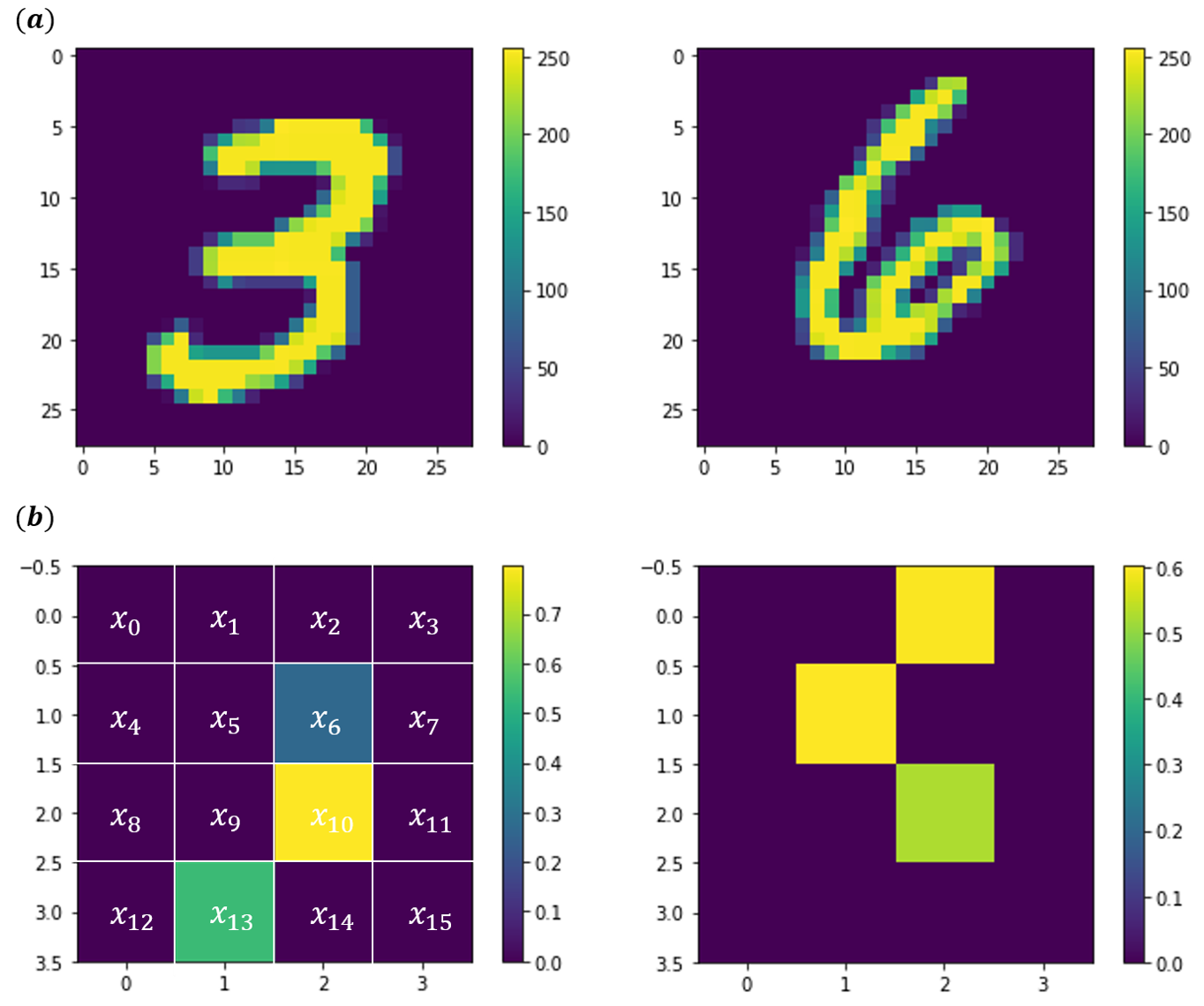
Figure 4: (a) The original images of numbers $3$ and $6$ have $28\times 28$ pixels. Each pixel has a value between $0$ to $255$. (b) The original images are rescaled to $4\times 4$ pixels and then normalized. Thus, $16$ amplitudes are generated and used to prepare quantum states.

References

- Biamonte et al. (2017) J. Biamonte, P. Wittek, N. Pancotti, P. Rebentrost, N. Wiebe, and S. Lloyd, Nature 549, 195 (2017).
- Maria Schuld (2018) F. P. Maria Schuld, Supervised Learning with Quantum Computers (Springer Cham, 2018).
- Dunjko et al. (2016) V. Dunjko, J. M. Taylor, and H. J. Briegel, Phys. Rev. Lett. 117, 130501 (2016).
- von Neumann (1932) J. von Neumann, Mathematical Foundations of Quantum Mechanics (Princeton University Press, 1932).
- Schuld and Killoran (2019) M. Schuld and N. Killoran, Phys. Rev. Lett. 122, 040504 (2019).
- Schuld (2021) M. Schuld, “Supervised quantum machine learning models are kernel methods,” arXiv:2101.11020 (2021).
- Pérez-García et al. (2006) D. Pérez-García, M. M. Wolf, D. Petz, and M. B. Ruskai, Journal of Mathematical Physics 47, 083506 (2006).
- Gleason (1957) A. Gleason, Indiana Univ. Math. J. 6, 885 (1957).
- Hong et al. (1987) C. K. Hong, Z. Y. Ou, and L. Mandel, Phys. Rev. Lett. 59, 2044 (1987).
- Horodecki and Ekert (2002) P. Horodecki and A. Ekert, Phys. Rev. Lett. 89, 127902 (2002).
- Helstrom (1969) C. W. Helstrom, Journal of Statistical Physics 1, 231 (1969).
- Ivanovic (1987) I. D. Ivanovic, Physics Letters A 123, 257 (1987).
- Dieks (1988) D. Dieks, Physics Letters A 126, 303 (1988).
- Peres (1988) A. Peres, Physics Letters A 128, 19 (1988).
- Bergou (2007) J. A. Bergou, Journal of Physics: Conference Series 84, 012001 (2007).
- Bae and Kwek (2015) J. Bae and L.-C. Kwek, Journal of Physics A: Mathematical and Theoretical 48, 083001 (2015).
- Croke et al. (2008) S. Croke, E. Andersson, and S. M. Barnett, Phys. Rev. A 77, 012113 (2008).
- Bae et al. (2011) J. Bae, W.-Y. Hwang, and Y.-D. Han, Phys. Rev. Lett. 107, 170403 (2011).
- Hwang and Bae (2010) W.-Y. Hwang and J. Bae, Journal of Mathematical Physics 51, 022202 (2010), https://doi.org/10.1063/1.3298647 .
- Jozsa and Schlienz (2000) R. Jozsa and J. Schlienz, Phys. Rev. A 62, 012301 (2000).
- Bae (2013) J. Bae, New Journal of Physics 15, 073037 (2013).
- Verstraete et al. (2001) F. Verstraete, J. Dehaene, and B. DeMoor, Phys. Rev. A 64, 010101 (2001).
- Verstraete and Wolf (2002) F. Verstraete and M. M. Wolf, Phys. Rev. Lett. 89, 170401 (2002).
- Bennett et al. (1996) C. H. Bennett, G. Brassard, S. Popescu, B. Schumacher, J. A. Smolin, and W. K. Wootters, Phys. Rev. Lett. 76, 722 (1996).
- Deutsch et al. (1996) D. Deutsch, A. Ekert, R. Jozsa, C. Macchiavello, S. Popescu, and A. Sanpera, Phys. Rev. Lett. 77, 2818 (1996).
- Popescu (1995) S. Popescu, Phys. Rev. Lett. 74, 2619 (1995).
- Lim et al. (2011) H.-T. Lim, Y.-S. Kim, Y.-S. Ra, J. Bae, and Y.-H. Kim, Phys. Rev. Lett. 107, 160401 (2011).
- Schuld et al. (2017) M. Schuld, M. Fingerhuth, and F. Petruccione, Europhysics Letters 119, 60002 (2017).
- Lloyd et al. (2021) S. Lloyd, M. Schuld, A. Ijaz, J. Izaac, and N. Killoran, “Quantum embeddings for machine learning,” arXiv:2001.03622 (2021).
- Farhi and Neven (2018) E. Farhi and H. Neven, “Classification with quantum neural networks on near term processors,” arXiv:1802.06002 (2018).