Scaling Down to Scale Up: A Guide to Parameter-Efficient Fine-Tuning

Abstract

This paper presents a systematic overview and comparison of parameter-efficient fine-tuning methods covering over 40 papers published between February 2019 and February 2023. These methods aim to resolve the infeasibility and impracticality of fine-tuning large language models by only training a small set of parameters. We provide a taxonomy that covers a broad range of methods and present a detailed method comparison with a specific focus on real-life efficiency and fine-tuning multibillion-scale language models.

1 Introduction

One thing that should be learned from the bitter lesson is the great power of general purpose methods, of methods that continue to scale with increased computation…

Rich Sutton, The Bitter Lesson

In October 2018, BERT Large Devlin et al. (2019) with 350 million parameters was the biggest Transformer model Vaswani et al. (2017) ever trained. At the time, contemporary hardware struggled to fine-tune this model. The section “Out-of-memory issues” on BERT’s GitHub specifies the maximum batch size for BERT Large given 12Gb of GPU RAM and 512 tokens as zero. Four years in, publically available models grew up to 176 billion parameters Scao et al. (2022); Zhang et al. (2022); Zeng et al. (2022), by a factor of 500. Published literature includes models up to 1 trillion parameters Chowdhery et al. (2022); Shoeybi et al. (2019); Fedus et al. (2021). However, single-GPU RAM increased less than 10 times (to 80Gb) due to the high cost of HBM memory. Model size scales almost two orders of magnitude quicker than computational resources making fine-tuning the largest models to downstream tasks infeasible for most and impractical for everyone.

In-context learning Radford et al. (2019) thus became the new normal, the standard way to pass downstream task training data to billion-scale language models. However, the limited context size of Transformers artificially limits the training set size to just a few examples, typically less than 100. This constraint, coupled with the absence of in-context learning performance guarantees even on the training data, presents a challenge. Additionally, expanding the context size leads to a quadratic increase in inference costs. Even though language models perform exceptionally well Brown et al. (2020) in a few-shot scenario, “get more data” is still the most reliable way to improve on any given task. Thus, we, as a community of researchers and engineers, need efficient ways to train on downstream task data.

Parameter-efficient fine-tuning, which we denote as PEFT, aims to resolve this problem by only training a small set of parameters which might be a subset of the existing model parameters or a set of newly added parameters. These methods differ in parameter efficiency, memory efficiency, training speed, final quality of the model, and additional inference costs (if any). In the last few years, more than a hundred of PEFT papers have been published, with several studies Ding et al. (2022) providing a good overview of the most popular methods, such as Adapters Houlsby et al. (2019), BitFit Ben-Zaken et al. (2021), LoRa Hu et al. (2021), Compacter Karimi Mahabadi et al. (2021), and Soft Prompts Liu et al. (2021); Li and Liang (2021). Recently, Pfeiffer et al. (2023) presented a survey on modular deep learning overviewing similar methods from the perspective of modularity and multi-task inference.

This survey presents a systematic overview, comparison, and taxonomy of 30 parameter-efficient fine-tuning methods with 20 methods discussed in-depth, covering over 40 papers published from February 2019 to February 2023. We highlight the current unresolved challenges in PEFT, including the limited theoretical understanding, the gap between PEFT and fine-tuning performance, and reporting issues. In conclusion, we suggest several avenues for improvement, such as developing standardized PEFT benchmarks, investigating novel reparameterization techniques with superior parameter-to-rank ratios, conducting in-depth studies on hyperparameters and interpretability, and drawing inspiration from on-device (edge) machine learning research.

2 Background: Transformer

Many of the parameter-efficient fine-tuning techniques discussed in this survey can be applied to all neural networks, but some are specifically designed to take advantage of the Transformer architecture Vaswani et al. (2017). Given that Transformers are the largest neural networks ever trained, these methods are particularly valuable. Thus, we present a brief overview of the Transformer to provide context for these techniques.

The core building block of the Transformer architecture consists of multi-head attention (MHA) followed by a fully-connected network (FFN), as illustrated in Figure 1. Both attention and fully-connected layers incorporate residual connections He et al. (2016) and Layer Normalization Ba et al. (2016) to improve trainability.

The heart of the Transformer is attention operation. Following the NamedTensor notation Chiang et al. (2021), it can be described as

$$\operatorname{Att}\colon\mathbb{R}^{\mathsf{\vphantom{fg}key}}\times\mathbb{R}^{\mathsf{\vphantom{fg}seq}\times\mathsf{\vphantom{fg}key}}\times\mathbb{R}^{\mathsf{\vphantom{fg}seq}\times\mathsf{\vphantom{fg}val}}\rightarrow\mathbb{R}^{\mathsf{\vphantom{fg}val}}$$

$$\operatorname{Att}(Q,K,V)=\left(\mathop{\underset{\begin{subarray}{c}\mathsf{\vphantom{fg}seq}\end{subarray}}{\vphantom{fg}\mathrm{softmax}}}\frac{Q\mathbin{\underset{\begin{subarray}{c}\mathsf{\vphantom{fg}key}\end{subarray}}{\vphantom{fg}\odot}}K}{\sqrt{|\mathsf{\vphantom{fg}key}|}}\right)\mathbin{\underset{\begin{subarray}{c}\mathsf{\vphantom{fg}seq}\end{subarray}}{\vphantom{fg}\odot}}V$$

$$Q(x) =x\cdot W_{Q}+b_{k},$$

$$K(x) =x\cdot W_{K}+b_{q},$$

$$V(x) =x\cdot W_{V}+b_{v},$$

$$W_{Q},\text{ }W_{K} \in\mathsf{\vphantom{fg}\mathbf{R}}^{\mathsf{\vphantom{fg}input}\times\mathsf{\vphantom{fg}key}},W_{V}\in\mathsf{\vphantom{fg}\mathbf{R}}^{\mathsf{\vphantom{fg}input}\times\mathsf{\vphantom{fg}val}}$$

$$b_{Q},\text{ }b_{K} \in\mathsf{\vphantom{fg}\mathbf{R}}^{\mathsf{\vphantom{fg}key}},\text{ }b_{V}\in\mathsf{\vphantom{fg}\mathbf{R}}^{\mathsf{\vphantom{fg}val}}$$

A number of methods act specifically on the matrices $W_{K}$, $W_{Q}$, $W_{V}$, as they provide the main mechanism to pass information from one token to another and control what information (value) is being passed.

Although specific implementations of the Transformer may vary, such as incorporating a cross-attention layer in seq2seq networks or using LayerNorm before sublayers (Pre-LN), most parameter-efficient fine-tuning methods for Transformers only rely on the basic MHA + FFN structure and can be readily adapted to architecture variations.

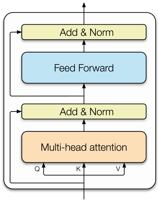
Figure 1: Basic Transformer block

3 Taxonomy of PEFT: a birds-eye view

PEFT methods can be classified in multiple ways. They may be differentiated by their underlying approach or conceptual framework: does the method introduce new parameters to the model, or does it fine-tune a small subset of existing parameters? Alternatively, they may be categorized according to their primary objective: does the method aim to minimize memory footprint or only storage efficiency? In this section, we begin by presenting a taxonomy based on the former. We depict this taxonomy and 30 PEFT methods in Figure 2. Sections 3.1-3.4 give a brief taxonomy overview. Then, based on our taxonomy classification, we describe 20 PEFT methods in detail, accompanied by the pseudocode in Sections 6 - 11.

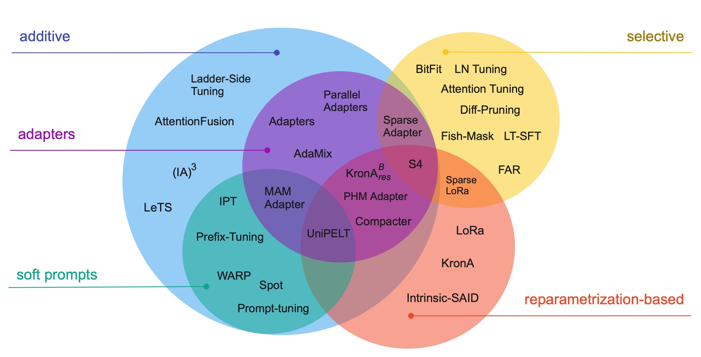
Figure 2: Parameter-efficient fine-tuning methods taxonomy. We identify three main classes of methods: Addition-based, Selection-based, and Reparametrization-based. Within additive methods, we distinguish two large included groups: Adapter-like methods and Soft prompts.

3.1 Additive methods

The main idea behind additive methods is augmenting the existing pre-trained model with extra parameters or layers and training only the newly added parameters. As of now, this is the largest and widely explored category of PEFT methods. Within this category, two large subcategories have emerged: Adapter-like methods and soft prompts.

Adapters

Adapters Houlsby et al. (2019) are a type of additive parameter-efficient fine-tuning method that involves introducing small fully-connected networks after Transformer sub-layers. The idea has been widely adopted Pfeiffer et al. (2020b) , and multiple variations of Adapters have been proposed. These variations include modifying the placement of adapters He et al. (2022a); Zhu et al. (2021), pruning He et al. (2022b), and using reparametrization to reduce the number of trainable parameters Karimi Mahabadi et al. (2021); Edalati et al. (2022).

Soft Prompts

Language model prompting Radford et al. (2019) aims to control the behavior of a language model by modifying the input text, which typically consists of a task description accompanied by a few in-context examples. However, these methods are difficult to optimize and are inherently limited in the number of training examples by the maximum model input length. To address these drawbacks, the concept of “soft” prompts was introduced Liu et al. (2021); Lester et al. (2021); Li and Liang (2021), where a part of the model’s input embeddings is fine-tuned via gradient descent. This pivots the problem of finding prompts in a discrete space to a continuous optimization problem. Soft prompts can be trained for the input layer only Liu et al. (2021); Lester et al. (2021) or for all layers Li and Liang (2021). Recent advancements explore how soft prompts could be pre-trained or prompts for different tasks utilized to reduce the computation required for fine-tuning a soft prompt for a new task Vu et al. (2021); Hambardzumyan et al. (2021); Su et al. (2021); Qin et al. (2021).

Other additive approaches

Additive methods are a diverse category of parameter-efficient fine-tuning techniques that extends beyond adapters and soft prompts. For example, LeTS Fu et al. (2021), LST Sung et al. (2022), and (IA)³ Liu et al. (2022) introduce novel ways to add parameters that improve adapters or soft prompts in terms of memory, computation, or accuracy.

Why add parameters?

Although these methods introduce additional parameters to the network, they achieve significant training time and memory efficiency improvements by reducing the size of the gradients and the optimizer states. Note that in the case of Adam Kingma and Ba (2015), for every byte of trainable parameter, one extra byte is needed for its gradient, and two more bytes are needed to store the optimizer state: the first and second moments of the gradient. In practice, depending on the setup, training a model requires 12-20 times more GPU memory than the model weights. By saving memory on optimizer states, gradients, and allowing frozen model parameters to be quantized Dettmers et al. (2022), additive PEFT methods enable the fine-tuning of much larger networks or the use of larger microbatch sizes. Which improves training throughput on GPUs. Moreover, optimizing fewer parameters in distributed setups drastically reduces communication volume.

Method	Type	Storage	Memory	Backprop	Inference overhead
Adapters Houlsby et al. (2019)	A	yes	yes	no	Extra FFN
AdaMix Wang et al. (2022)	A	yes	yes	no	Extra FFN
SparseAdapter He et al. (2022b)	AS	yes	yes	no	Extra FFN
Cross-Attn tuning Gheini et al. (2021)	S	yes	yes	no	No overhead
BitFit Ben-Zaken et al. (2021)	S	yes	yes	no	No overhead
DiffPruning Guo et al. (2020)	S	yes	no	no	No overhead
Fish-Mask Sung et al. (2021)	S	yes	maybe	no	No overhead
LT-SFT Ansell et al. (2022)	S	yes	maybe	no	No overhead
Prompt Tuning Lester et al. (2021)	A	yes	yes	no	Extra input
Prefix-Tuning Li and Liang (2021)	A	yes	yes	no	Extra input
Spot Vu et al. (2021)	A	yes	yes	no	Extra input
IPT Qin et al. (2021)	A	yes	yes	no	Extra FFN and input
MAM Adapter He et al. (2022a)	A	yes	yes	no	Extra FFN and input
Parallel Adapter He et al. (2022a)	A	yes	yes	no	Extra FFN
Intrinsinc SAID Aghajanyan et al. (2020)	R	no	no	no	No overhead
LoRa Hu et al. (2021)	R	yes	yes	no	No overhead
UniPELT Mao et al. (2021)	AR	yes	yes	no	Extra FFN and input
Compacter Karimi Mahabadi et al. (2021)	AR	yes	yes	no	Extra FFN
PHM Adapter Karimi Mahabadi et al. (2021)	AR	yes	yes	no	Extra FFN
KronA Edalati et al. (2022)	R	yes	yes	no	No overhead
KronA${}^{B}_{res}$ Edalati et al. (2022)	AR	yes	yes	no	Extra linear layer
(IA)3 Liu et al. (2022)	A	yes	yes	no	Extra gating
Attention Fusion Cao et al. (2022)	A	yes	yes	yes	Extra decoder
LeTS Fu et al. (2021)	A	yes	yes	yes	Extra FFN
Ladder Side-Tuning Sung et al. (2022)	A	yes	yes	yes	Extra decoder
FAR Vucetic et al. (2022)	S	yes	maybe	no	No overhead
S4-model Chen et al. (2023)	ARS	yes	yes	no	Extra FFN and input

Table 1: Comparing PEFT methods across storage efficiency, memory efficiency, and computational efficiency in terms of reducing backpropagation costs and having inference overhead. Method types: A – additive, S – selective, R – reparametrization-based.

3.2 Selective methods

Arguably the earliest example of selective PEFT is fine-tuning only a few top layers of a network Donahue et al. (2014). Modern approaches are usually based on the type of the layer Gheini et al. (2021) or the internal structure, such as tuning only model biases Ben-Zaken et al. (2021) or only particular rows Vucetic et al. (2022).

An extreme version of selective methods is sparse update methods which can completely ignore the structure of the model, and select parameters individually Sung et al. (2021); Ansell et al. (2022); Guo et al. (2020). However, sparse parameter updates present multiple engineering and efficiency challenges, some of which have been tackled in recent research on parameter reconfiguration Vucetic et al. (2022) (Section 9.3) and NxM sparsity Holmes et al. (2021). Nevertheless, unrestricted unstructured sparsity is still impractical on contemporary hardware.

3.3 Reparametrization-based methods

Reparametrization-based parameter-efficient fine-tuning methods leverage low-rank representations to minimize the number of trainable parameters. The notion that neural networks have low-dimensional representations has been widely explored in both empirical and theoretical analysis of deep learning Maddox et al. (2020); Li et al. (2018); Arora et al. (2018); Malladi et al. (2022).

Aghajanyan et al. (2020) have demonstrated that fine-tuning can be performed effectively in low-rank subspaces. Further, they showed that the size of the subspace that needs adaption is smaller for bigger models or the models pre-trained for longer. Their approach, referred to as Intrinsic SAID (Section 10.1), employs the Fastfood transform Le et al. (2013) to reparametrize the update to neural network parameters.

However, perhaps the most well-known reparametrization-based method is Low-Rank Adaptation or LoRa Hu et al. (2021), which employs a simple low-rank matrix decomposition to parametrize the weight update $\delta W=W^{\text{down}}W^{\text{up}}$. This approach is straightforward to implement and has been evaluated on models with up to 175 billion parameters. We provide a detailed discussion of this method in Section 10.2. More recent works Karimi Mahabadi et al. (2021); Edalati et al. (2022) have also explored the use of Kronecker product reparametrization ($\delta W=A\otimes B$), which yields a more favorable tradeoff between rank and parameter count.

3.4 Hybrid methods

A number of methods have emerged that combine ideas from multiple categories of PEFT He et al. (2022a, b); Mao et al. (2021); Karimi Mahabadi et al. (2021). For instance, MAM Adapter (Section 11.2) incorporates both Adapters and Prompt tuning. UniPELT (Section 11.3) adds LoRa to the mixture. Compacter and KronA${}^{B}_{res}$ reparametrize the adapters to reduce their parameter count (Sections 11.4 and 10.3). Finally, S4 (Section 11.5) is a result of an automated algorithm search that combines all PEFT classes to maximize accuracy at $0.5\%$ of extra parameter count.

Method	% Trainable parameters	% Changed parameters	Evaluated on
			<1B	<20B	>20B
Adapters Houlsby et al. (2019)	0.1 - 6	0.1 - 6	yes	yes	yes
AdaMix Wang et al. (2022)	0.1 - 0.2	0.1 - 0.2	yes	no	no
SparseAdapter He et al. (2022b)	2.0	2.0	yes	no	no
BitFit Ben-Zaken et al. (2021)	0.05 - 0.1	0.05 - 0.1	yes	yes	yes
DiffPruning Guo et al. (2020)	200	0.5	yes	no	no
Fish-Mask Sung et al. (2021)	0.01 - 0.5	0.01 - 0.5	yes	yes	no
Prompt Tuning Lester et al. (2021)	0.1	0.1	yes	yes	yes
Prefix-Tuning Li and Liang (2021)	0.1 - 4.0	0.1 - 4.0	yes	yes	yes
IPT Qin et al. (2021)	56.0	56.0	yes	no	no
MAM Adapter He et al. (2022a)	0.5	0.5	yes	no	no
Parallel Adapter He et al. (2022a)	0.5	0.5	yes	no	no
Intrinsinc SAID Aghajanyan et al. (2020)	0.001 - 0.1	$\mathord{\sim}$0.1 or 100	yes	yes	no
LoRa Hu et al. (2021)	0.01 - 0.5	$\mathord{\sim}$0.5 or $\mathord{\sim}$30	yes	yes	yes
UniPELT Mao et al. (2021)	1.0	1.0	yes	no	no
Compacter Karimi Mahabadi et al. (2021)	0.05-0.07	$\mathord{\sim}$0.07 or $\mathord{\sim}$0.1	yes	yes	no
PHM Adapter Karimi Mahabadi et al. (2021)	0.2	$\mathord{\sim}$0.2 or $\mathord{\sim}$1.0	yes	no	no
KronA Edalati et al. (2022)	0.07	$\mathord{\sim}$0.07 or $\mathord{\sim}$30.0	yes	no	no
KronA${}^{B}_{res}$ Edalati et al. (2022)	0.07	$\mathord{\sim}$0.07 or $\mathord{\sim}$1.0	yes	no	no
(IA)3 Liu et al. (2022)	0.02	0.02	no	yes	no
Ladder Side-TuningSung et al. (2022)	7.5	7.5	yes	yes	no
FAR Vucetic et al. (2022)	6.6-26.4	6.6-26.4	yes	no	no
S4-model Chen et al. (2023)	0.5	more than 0.5	yes	yes	no

Table 2: What model sizes PEFTmethods have been evaluated on and their typical amount of trainable parameters used in the papers. By trainable parameter count we specifically mean the number parameters that are updated by a gradient optimization algorithm, not the delta between the original and final model which we denote “changed parameters”. For reprametrization-based method we report parameters before and after reparametrization. Estimating updated parameter count for S4 is complicated as the model uses different methods at different layers. We report the range at which the methods were evaluated in the published literature.

4 Comparing PEFT methods

Parameter efficiency encompasses multiple aspects, including storage, memory, computation, and performance. However, achieving parameter efficiency alone does not necessarily lead to reduced RAM usage. For example, DiffPruning (Section 9.2) entails training a binary mask with the same number of parameters as the model. Consequently, this method can be only considered storage-efficient, while still incurring considerable RAM and time costs during fine-tuning.

To compare PEFT methods, we keep five dimensions of comparison in mind: storage efficiency, memory efficiency, computation efficiency, accuracy, and inference overhead. We observe that while they aren’t completely independent from one another, improvements along one of the axes do not necessarily translate into improvements along others (Table 1).

5 Overview of PEFT Approaches

In the next sections, we dive into the details of several parameter-efficient fine-tuning approaches. We will describe the distinctions and tradeoffs between them in terms of the axes outlined in Section 4. We bold a one-sentence summary of each method to simplify skimming through them.

In the method description, we also indicate whether it has been applied to models with fewer than 1 billion, fewer than 20 billion, or more than 20 billion parameters. The model size summary can be found in Table 2. We stick to the parameter counts indication where possible because the words “small” and “large” change their meaning too quickly. Finally, we provide a brief pseudo-PyTorch implementation of the most important part of the algorithm where it’s feasible.

6 Additive methods: Adapters

We start our dive into PEFT methods with one of the largest sub-families of methods that are built on the idea of adding fully-connected networks between model layers, i.e., adapters.

6.1 Adapters

The idea of Adapters was initially developed for multi-domain image classification Rebuffi et al. (2017, 2018) and consisted in adding domain-specific layers between neural network modules.

Houlsby et al. (2019) adapt this idea to NLP. They propose to add fully-connected networks after attention and FFN layers in Transformer. Unlike the transformer FFN block, Adapters usually have a smaller hidden dimension than the input. Adapters have demonstrated impressive parameter efficiency at the time, showing that it is possible to achieve performance competitive to full fine-tuning by tuning less than 4% of the total model parameters.

A schematic adapter implementation:

⬇

def transformer_block_with_adapter(x):

residual = x

x = SelfAttention(x)

x = FFN(x) # adapter

x = LN(x + residual)

residual = x

x = FFN(x) # transformer FFN

x = FFN(x) # adapter

x = LN(x + residual)

return x

Pfeiffer et al. (2020a) found that inserting the adapter only after the self-attention layer (after normalization) achieves similar performance as using two adapters per transformer block.

6.2 AdaMix

AdaMix Wang et al. (2022) improves the performance of adapters by utilizing multiple adapters in a mixture-of-experts (MoE) fashion Shazeer et al. (2017). Meaning, that each adapter layer is a set of layers (experts), and for each forward pass only a small set of experts is activated. In contrast to a regular MoE, which selects and weights multiple experts using a routing network AdaMix randomly selects a single expert for each forward pass. This minimizes computational costs and, according to Wang et al. (2022), doesn’t degrade performance. Another difference from a regular MoE layer is that up and down projections of the adapter are selected independently. After training, the adapter weights are averaged across the experts which makes inference more memory-efficient. To stabilize training, the authors propose consistency regularization which minimizes symmetrized $KL$ between two models’ forwards with different sets of experts selected.

Although AdaMix achieves better performance than regular adapters with the same inference cost, it can use more memory during training. Wang et al. (2022) show that AdaMix can use much smaller adapter hidden states, which amortizes trainable parameter overhead over the number of experts ($\sim$4-8). However, the consistency regularization technique increases computational requirements and memory consumption, as it needs to keep two versions of the hidden states and gradients over two model forward passes with different experts.

⬇

def transformer_block_with_adamix(x):

residual = x

x = SelfAttention(x)

x = LN(x + residual)

residual = x

x = FFN(x)

# adamix starts here

x = random_choice(experts_up)(x)

x = nonlinearity(x)

x = random_choice(experts_down)(x)

x = LN(x + residual)

return x

def consistency_regularization(x):

logits1 = transformer_adamix(x)

# second pass uses different experts

logits2 = transformer_adamix(x)

r = symmetrized_KL(logits1, logits2)

return r

7 Additive Methods: Soft Prompts

Prompting language models has demonstrated remarkable performance in zero- and few-shot scenarios Brown et al. (2020); Schick and Schütze (2021). However, optimizing discrete natural language prompts or using in-context learning is impractical when there are many training examples. To overcome this challenge, the concept of “soft” or “continuous” prompts was proposed Li and Liang (2021); Lester et al. (2021); Liu et al. (2021) that converts the discrete optimization problem of finding the best "hard" prompt to a continuous one.

7.1 Prompt Tuning

Prompt tuning Lester et al. (2021) proposes to prepend the model input embeddings with a trainable tensor $\mathbf{P}\in\mathsf{\vphantom{fg}\mathbf{R}}^{l\times h}$. This tensor is commonly referred to as “soft prompt” and it is optimized directly through gradient descent.

⬇

def soft_prompted_model(input_ids):

x = Embed(input_ids)

x = concat([soft_prompt, x], dim=seq)

return model(x)

Ablation studies by Su et al. (2021) over prompt length from 1 to 150 tokens and model size from 10M to 11B parameters reveal that prompt tuning is more parameter efficient the larger the model. For instance, prompt tuning of T5-11B achieves the same SuperGLUE Wang et al. (2019) performance with either 5 or 150 soft prompt length.

Furthermore, efficiency grows faster than the model size: T5-large performance saturates at prompt length 20 or 20K trainable parameters ($0.002\%$), and T5-XL performance saturates prompt length 5, also 20K trainable parameters ($0.0002\%$). However, prompt tuning only becomes comparable with full fine-tuning at the 10B model scale. Also, increasing the length of the input by 20-100 tokens can significantly increase computation, given the quadratic complexity of the transformer. Overall, soft prompts are incredibly parameter-efficient at the cost of inference overhead and more applicable to larger models.

7.2 Prefix-Tuning

Li and Liang (2021) independently develop the idea of soft prompts with a distinctive flavor: instead of adding a soft prompt to the model input, trainable parameters are prepended to the hidden states of all layers. The same prefix $\mathbf{P}_{\theta}\in\mathsf{\vphantom{fg}\mathbf{R}}^{l\times h}$ is prepended to all of the hidden states.

They observe that directly optimizing the soft prompt leads to instabilities during training. Instead, soft prompts are parametrized through a feed-forward network $\mathbf{P}_{\theta}=\operatorname{FFN}(\hat{\mathbf{P}}_{\theta})$. During training, $\hat{\mathbf{P}}_{\theta}$ and the parameters of the FFN are optimized. After, only $\mathbf{P}_{\theta}$ is needed for inference, and the FFN can be discarded.

Pseudocode for a single layer:

⬇

def transformer_block_for_prefix_tuning(x):

soft_prompt = FFN(soft_prompt)

x = concat([soft_prompt, x], dim=seq)

return transformer_block(x)

Note that the approach is very similar to Prompt-tuning (Section 7.1), but the soft prompts are added in each layer.

In their experiments, Li and Liang (2021) apply BART Lewis et al. (2019) model (<1B) to different generation tasks and show a performance close to the full fine-tuning by training only $0.1\%$ parameters. Soft prompt lengths used in the study vary from 10 to 200 tokens.

7.3 Intrinsic Prompt Tuning (IPT)

Prompt tuning methods, despite being parameter efficient, present practical problems such as slow convergence and a need to store all of the task-specific parameters. A few studies Su et al. (2021); Vu et al. (2021) proposed to pre-train soft prompts to improve performance and convergence speed. However, these methods do not provide solutions to reduce the number of parameters per task.

Qin et al. (2021) hypothesize that the h-dimensional space used to define soft prompt parameters contains an “intrinsic task subspace” that can differentiate between various tasks.

IPT method works in three steps. First, given a set of training tasks, their soft prompts are learned in a regular way (Section 7.1). Then, these prompts are used to train an autoencoder that compresses their dimensionality. After this, the encoder part is discarded, and only the input to the autoencoder decoder is trained on new tasks. In summary, IPT uses an autoencoder to (de)compress the soft prompt.

⬇

def autoencoder(soft_prompt):

soft_prompt = soft_prompt.flatten()

P = FFN_A(soft_prompt) # encoder

P = FFN_B(P) # decoder

P = P.reshape(prompt_len, hidden)

return P

def soft_prompted_model(x):

P = FFN_B(intrinsic_subspace_prompt)

P = P.reshape(prompt_len, hidden)

x = concat([P, x], dim=seq)

return model(x)

Even though the IPT framework reduces the number of parameters for the unseen tasks, this reduction comes at the price of training the autoencoder. The authors conduct experiments with the BART-base model and a prompt length of 100. The resulting autoencoder, which is implemented as a fully-connected network that accepts a one-dimensional tensor of size $768\cdot 100$ reaches approximately 78 million parameters. I.e., over 56% of total parameters in the BART-base model. Hence, significantly more efficient ways of prompt autoencoding are required to make IPT practically applicable.

8 Additive Methods: Other Approaches

Several of the additive PEFT methods do not follow the idea of either adapters or soft prompts and propose to augment a pre-trained network in an original way.

8.1 Ladder-Side Tuning (LST)

Ladder-Side Tuning Sung et al. (2022) trains a small transformer network on the side of the pre-trained network. This side network combines the hidden states of the pre-trained backbone network with its own hidden states.

This way, the side network only uses the pre-trained model as a feature extractor, and backpropagation must only be computed through the side network saving on both memory and compute during training. The authors also use multiple tricks no improve the performance and parameter efficiency of LST. Namely, initializing the side network from the pre-trained model parameters using structural pruning and using twice (or 4x) fewer layers in the side network than in the backbone network.

The pseudocode:

⬇

def ladder_side_layer(x, h_pt):

h_pt = h_pt @ W_down # to x.shape

gate = sigmoid(alpha)

x = gate * x + (1 - gate) * h_pt

return transformer_block(x)

def ladder_side_network(x):

with no_grad():

H_pt = pretrained_network(

x, return_all_hiddens=True

)

for i in range(layers):

layer = ladder_side_layers[i]

x = layer(x, H_pt[i])

return x

Where h_pt is the output of the corresponding layer of the pre-trained network, and alpha is an input-independent trainable scalar gate.

LST demonstrated a three-fold RAM reduction in fine-tuning T5-Base compared to full fine-tuning and a two-fold RAM usage reduction compared to LoRa (Section 10.2) with a small degradation in accuracy and outperforms these methods when controlling for RAM usage.

8.2 (IA)³

Liu et al. (2022) propose a new parameter-efficient method to multi-task fine-tune T-few. (IA)³ learns new parameters $l_{v}$, $l_{k}$, $l_{ff}$ which rescale key, value, and hidden FFN activations. Specifically,

⬇

def transformer_block_with_ia3(x):

residual = x

x = ia3_self_attention(x)

x = LN(x + residual)

residual = x

x = x @ W_1 # FFN in

x = l_ff * gelu(x) # (IA)3 scaling

x = x @ W_2 # FFN out

x = LN(x + residual)

return x

def ia3_self_attention(x):

k, q, v = x @ W_k, x @ W_q, x @ W_v

k = l_k * k

v = l_v * v

return softmax(q @ k.T) @ V

Training only these three vectors $l_{v}$, $l_{k}$, $l_{ff}$ for each transformer block leads to high parameter efficiency. For T0-3B, it only updates about $0.02\%$ of model parameters and outperforms other methods, including Compacter (Section 11.4) with similar parameter count and LoRa (Section 10.2) with 16 times more trainable parameters. Unlike adapters-tuned models, (IA)³-tuned models exhibit minimal overhead. Vectors $l_{v}$ and $l_{k}$ can be integrated into the corresponding linear layers, and the only overhead comes from $l_{ff}$.

9 Selective Methods

Selective methods fine-tune a subset of the existing parameters of the model. It could be a layer depth-based selection, layer type-based lection, or even individual parameter selection.

9.1 BitFit

Ben-Zaken et al. (2021) propose to only fine-tune the biases of the network. That is, for every linear or convolutional layer, the weight matrix $W$ is left as is, and only the bias vector $b$ is optimized.

⬇

params = (p for n, p

in model.named_parameters()

if "bias" in n)

optimizer = Optimizer(params)

BitFit only updates about 0.05% of the model parameters. The original paper demonstrated that the method achieves similar performance to full fine-tuning or better performance in low and medium-data scenarios in BERT models (<1B parameters). Further research evaluated the method on larger networks such as T0-3B Sanh et al. (2022); Liu et al. (2022) or GPT-3 Hu et al. (2021). At this scale, BitFit significantly underperforms full fine-tuning, and other PEFT approaches.

9.2 DiffPruning

DiffPruning Guo et al. (2020) aims to achieve parameter efficiency by learning a sparse update of a neural network’s weights. The method introduces a learnable binary mask on the weights, denoted by $\delta=z\circ\Delta W$, where $\circ$ represents the Hadamard product. This parameter mask is learned during model fine-tuning as part of the regularization objective, which is a differentiable approximation to the $L_{0}$ norm of the update vector $\delta$.

DiffPruning has achieved comparable performance to full fine-tuning while modifying only 0.5% of the model parameters in smaller-scale (<1B) scenarios. This makes it a useful method for multi-task deployment for edge (mobile) scenarios where storage is limited. However, this method requires more memory than traditional fine-tuning, as it involves optimizing all parameters during training in addition to the learnable binary mask.

9.3 Freeze and Reconfigure (FAR)

FAR Vucetic et al. (2022) selects columns of parameter matrices to prune and reconfigures linear layers into trainable and frozen. The method operates in two stages. In the first stage, the most important rows of parameter matrices are identified for updating. This process is similar to structured pruning and can use any pruning method. In their paper, the authors fine-tune the model on a percentage of the data and select the top-$r$ rows based on the $L_{1}$ distance between the fine-tuned and original models.

In the second stage, the network is reconfigured by splitting each parameter $W\in\mathbb{R}^{in\times h}$ into a trainable component $W_{t}\in\mathbb{R}^{in\times h^{\prime}}$ and a frozen component $W_{f}\in\mathbb{R}^{in\times(h-h^{\prime})}$, where $h^{\prime}$ is the desired number of trainable parameters. The matrix multiplications with $W_{t}$ and $W_{f}$ are computed independently, and the results are concatenated. A similar operation is performed on biases.

Pseudocode implementation is rather simple

⬇

def far_layer(x):

h1 = x @ W_t

h2 = x @ W_f

return concat([h1, h2], dim=-1)

While this approach creates additional compute overhead during training, it provides great flexibility in terms of parameter selection on modern hardware using standard frameworks like PyTorch. After training, the parameters can be reconfigured back removing any inference overhead.

The original paper focused on edge scenarios and used DistilBERT (66M) for their experiments. FAR was only applied to feed-forward layers, as these make up the majority of the DistilBERT parameters. The authors showed that FAR achieved similar performance to fine-tuning on five GLUE tasks and SQuAD 2.0 Rajpurkar et al. (2018) while updating 6% of the parameters.

9.4 FishMask

FishMask Sung et al. (2021) is a sparse fine-tuning method that selects top-p parameters of the model based on their Fisher information. Fisher information is estimated in a common way through a diagonal approximation

$$\hat{F_{\theta}}=\frac{1}{N}\sum_{i=1}^{N}\mathbb{E}_{y\sim p_{\theta}(y|x_{i})}(\nabla_{\theta}\log p_{\theta}(y|x_{i}))^{2}$$

Thus, the method requires computing gradients for all parameters on (several batches of) the data. However, after the highest-Fisher parameters are selected, only they need to be optimized.

Pseudocode to compute the masks:

⬇

sparsity = 0.99

N = len(data)

for x, y in data:

loss = loss_fn(model(x), y)

loss.backward()

for n, p in model.named_params():

fisher[n] += p.grad ** 2 / N

threshold = percentile(fisher, sparsity)

masks = {n: f > threshold

for n, f in fisher.items()}

The method generally performs on-par with adapters but sub-par to LoRa and (IA)³ (Sections 10.2 and 8.2). It has been evaluated on BERT (<1B) and T0-3B models. However, FishMask is computationally intensive and inefficient on contemporary deep learning hardware due to the lack of support for sparse operations.

10 Reparametrization-based methods

These methods use the idea of reparametrizing the weights of the network using a low-rank transformation. This decreases the trainable parameter count while still allowing the method to work with high-dimensional matrices, such as the pre-trained parameters of the networks.

10.1 Intrinsic SAID

In their work, Aghajanyan et al. (2020) investigate the intrinsic dimensionality of fine-tuning and demonstrate that this process can be performed in a low-rank subspace. Specifically, they use the Fastfood transform to reparametrize the update to the model weights. Fastfood is a compute-efficient dimensionality expansion transform $F:\mathsf{\vphantom{fg}\mathbf{R}}^{d}\rightarrow\mathsf{\vphantom{fg}\mathbf{R}}^{D}$ that can be done in $O(D\log d)$ time and $O(D)$ memory.

Their results indicate that larger models require changes in a lower-rank subspace compared to smaller models to achieve the same fine-tuning performance. This observation motivates both scaling large models and parameter-efficient fine-tuning. It is important to note that, unlike methods that select a particular subset of parameters for fine-tuning, Intrinsic SAID updates all model parameters in a low-rank manner, i.e., $\theta=\theta_{0}+F(\theta^{d})$, where $\theta_{0}\in\mathsf{\vphantom{fg}\mathbf{R}}^{D}$ denotes the pre-trained model parameters and $\theta^{d}\in\mathsf{\vphantom{fg}\mathbf{R}}^{d}$ denotes the parameters to be optimized. Therefore, while the number of optimizable parameters is low, the $O(D)$ memory complexity of Fastfood and the update to all of the model’s parameters make Intrinsic SAID impractical for fine-tuning large networks. For more details on Fastfood, we refer the reader to the original paper by Le et al. (2013).

10.2 LoRa

LoRa Hu et al. (2021) takes inspiration from IntrinsicSAID and proposes a simpler way to perform low-rank fine-tuning. Parameter update for a weight matrix in LoRa is decomposed into a product of two low-rank matricies

$$\delta W =W_{A}W_{B}$$ (1)

$$W_{A} \in\mathsf{\vphantom{fg}\mathbf{R}}^{\text{in}\times r},W_{B}\in\mathsf{\vphantom{fg}\mathbf{R}}^{r\times\text{out}}$$

All pre-trained model parameters are kept frozen, and only $W_{A}$ and $W_{B}$ matrices are trainable. The scaling factor is constant and typically equals $\frac{1}{r}$. After training, they can be integrated into the original $W$ by just adding the matrix $W_{A}W_{B}$ to the original matrix $W$.

Pseudocode is very simple:

⬇

def lora_linear(x):

h = x @ W # regular linear

h += x @ W_A @ W_B # low-rank update

return scale * h

In Transformers, LoRa is typically used for $W_{K}$ and $W_{V}$ projection matrices in multi-head attention modules. The method outperforms BitFit and Adapters and has been evaluated on the models up to 175B parameters.

10.3 KronA

KronA Edalati et al. (2022) replaces matrix factorization $\delta W=W_{A}W_{B}$ in LoRa (Section 10.2) with a matrix factorization through a Kronecker product $\delta W=W_{A}\otimes W_{B}$. This yields a better rank per parameters tradeoff because the Kronecker product keeps the rank of the original matrices being multiplied. Or, in other words, $\operatorname{rank}(A\otimes B)=\operatorname{rank}A\cdot\operatorname{rank}B$. Additionally, Edalati et al. (2022) propose to use efficient Kronecker product-vector product operation $x(A\otimes B)$ which avoids representing $\delta W$ explicitly and leads to significant speedups

Krona pseudocode:

⬇

def krona_linear(x):

x = x @ W # regular linear

x += kronecker_vector_prod(x, W_A, W_B)

return scale * x

# same as x @ kronecker_product(A, B)

def kronecker_vector_prod(x, A, B):

x = x.reshape(A.shape[1], B.shape[1])

x = A.T @ x @ B

return x.reshape(-1)

KronA${}^{B}_{res}$ is another method presented in Edalati et al. (2022). It is a parallel adapter with Kronecker product-parametrization of the weights and a residual connection.

On GLUE, KronA methods perform on-par or better than adapters (Section 6.1), LoRa (Section 10.2), and Compacter (Section 11.4) at the same trainable parameter count $0.07\%$ while being significantly faster than adapters or Compacter at inference time. The method was evaluated only on small (<1B) models.

Background: What is a Kronecker product?

Kronecker product is a tensor operation defined as

$$\mathbf{A}\otimes\mathbf{B} :\mathsf{\vphantom{fg}\mathbf{R}}^{n\times m}\times\mathsf{\vphantom{fg}\mathbf{R}}^{k\times l}\rightarrow\mathsf{\vphantom{fg}\mathbf{R}}^{nk\times ml}$$ (2)

$$\mathbf{A}\otimes\mathbf{B} =\begin{bmatrix}a_{1,1}\mathbf{B}&\cdots&a_{1,n}\mathbf{B}\\ \vdots&\ddots&\vdots\\ a_{m,1}\mathbf{B}&\cdots&a_{m,n}\mathbf{B}\end{bmatrix}$$

It can be easily implemented in PyTorch using the command torch.einsum

⬇

def batched_kronecker_product(a, b):

bs, i, j = a.shape

bs, k, m = b.shape

res = einsum("bij,bkm->bikjm", a, b)

return res.view(bs, i * k, j * m)

11 Hybrid Approaches

Hybrid methods for parameter-efficient fine-tuning combine different techniques and strategies to achieve better performance while reducing the computational costs associated with fine-tuning large neural networks. These methods can be viewed as a synergistic blend of multiple approaches. The resulting hybrid methods can leverage the strengths of each individual technique, while mitigating their weaknesses, leading to improved performance and efficiency.

11.1 SparseAdapter

He et al. (2022b) propose Large-Sparse strategy to train adapter layers. In this strategy, they use a large hidden dimension for the added module and prune around 40% of the values at initialization. Large-Sparse consistently outperforms its non-sparse counterpart with the same trainable parameter count. However, training and inference costs can be higher depending on hardware support for sparse tensors and operations. It is also worth noting that computing the pruning mask for this method may require obtaining gradients for all newly added parameters.

11.2 MAM Adapters

In their study, He et al. (2022a) conducted a thorough investigation of adapter placement and soft prompts. They concluded that scaled parallel adapters outperform sequentially-placed adapters and that placing an adapter in parallel to FFN outperforms multi-head attention-parallel adapters. They also notice that soft prompts can efficiently modify attentions by only changing 0.1% of the parameters and propose to “mix-and-match” (MAM) these ideas. Their final model, MAM Adapter is a combination of scaled parallel adapter for FFN layer and soft prompt.

⬇

def transformer_block_mam(x):

x = concat([x, soft_prompt], dim=seq)

residual = x

x = SelfAttention(x)

x = LN(x + residual)

x_a = FFN(x) # parallel adapter

x_a = scale * x_a

x = LN(x + x_adapter)

return x

MAM method outperforms BitFit and PromptTuning by a large margin and consistently outperforms LoRa (Section 10.2), Adapters (Section 6.1), and Prefix Tuning (Section 7.2) with 200 soft prompt length at 7% extra parameters. The experiments were concluded on <1B models.

It’s worth noting that parallel adapters were independently studied by Zhu et al. (2021) in the domain of machine translation.

11.3 UniPELT

UniPELT Mao et al. (2021) is a gated combination of LoRa, Prefix-tuning, and Adapters. More specifically, LoRa reparametrization is used for $W_{Q}$ and $W_{V}$ attention matrices, prefix-tuning is applied to keys and values of each layer, and adapters are added after the feed-forward layer of the transformer block. For each of the modules, gating is implemented as a linear layer projecting the module input into a dimension of size one, sigmoid activation, and averaging the resulting vector over the sequence length. Trainable parameters include LoRa matrices $W_{A},W_{B}$, prompt tuning parameters $P_{q},P_{k}$, adapter parameters, and gating function weights.

Next, we present a schematic implementation of UniPELT. We omit multiple attention heads for simplicity.

⬇

def transformer_block_with_unipelt(x):

residual = x

x = unipelt_self_attention(x)

x = LN(x + residual)

residual = x

x = FFN(x)

adapter_gate = gate(x)

x = adapter_gate * FFN(x)

x = LN(x + residual)

return x

def unipelt_self_attention(x):

k, q, v = x @ W_k, x @ W_q, x @ W_v

# lora for queries and values

lora_gate = gate(x)

q += lora_gate * W_qA @ W_aB

v += lora_gate * W_vA @ W_vB

# prefix tuning

pt_gate = gate(x)

q_prefix = pt_gate * P_q

k_prefix = pt_gate * P_k

return softmax(q @ k.T) @ V

def gate(x):

x = Linear(x)

x = sigmoid(x)

return mean(x, dim=seq)

UniPELT demonstrates significant improvements over individual LoRa, Adapters, and Prefix Tuning approaches in low-data scenarios with only 100 examples. In higher data scenarios, UniPELT performs on par or better than these approaches. Mao et al. (2021) reports 1.3% trainable model parameters using UniPELT on BERT (<1B parameters) models.

11.4 Compacter

Compacter Karimi Mahabadi et al. (2021) utilizes Kronecker product, low-rank matrices, and parameter sharing across layers to produce adapter weights. Each parameter $W$ in an adapter is equal to a sum of Kronecker products

$$\hat{W} =\sum_{i=0}^{n}A_{i}\otimes B_{i}$$ (3)

$$\hat{W}\in\mathsf{\vphantom{fg}\mathbf{R}}^{k\times d},\text{ } A_{i}\in\mathsf{\vphantom{fg}\mathbf{R}}^{n\times n},\text{ }B_{i}\in\mathsf{\vphantom{fg}\mathbf{R}}^{\frac{k}{n}\times\frac{d}{n}}.$$

A linear layer $x\hat{W}+b$ with this parametrization is called parametrized hypercomplex multiplication (PHM) layer Zhang et al. (2021). Compacter takes this idea futher, parametrizing $B_{i}$ similar to LoRa (Section 10.2) $B_{i}=B_{i}^{\text{down}}B_{i}^{\text{up}}$ where all matricies are of rank at most $r$. Matrices $A_{i}$ are shared across all adapter layers for further parameter efficiency. The corresponding layer is named Low-rank PHM or LPHM. Compacter layer pseudocode:

⬇

def compacter(x):

x = LPHM(x) # Essentially an FFN

x = gelu(x) # but

x = LPHM(x) # LPHM replaces linear

return x

def lphm_forward(x):

B = B_d @ B_u

W = batched_kronecker_product(A, B)

W = sum(W, dim=0)

return x @ W + b

Note that all $A$ and $B$ are 3D tensors with the first dimension equal to $n$, the number of Kronecker products in the PHM layer.

Compacter comes in two flavors: two adapters per transformer block or a single adapter after a feedforward layer (Compacter++). With only 0.05% additional parameters Compacter++ performs on par or better than adapters with 0.8% additional parameters. The model has been evaluated on T5 Base (<1B) and T0-3B.

11.5 S4

Chen et al. (2023) conduct an extensive exploration of various combinations of parameter-efficient fine-tuning techniques. Their search space includes dividing consecutive layers into four uneven groups, allocating varying amounts of trainable parameters to each layer, determining which groups to fine-tune, and deciding which PEFT methods to apply to each group.

Their proposed method, S4, divides layers into four groups ($G_{1,2,3,4}$) using a “spindle” pattern: more layers are allocated to the middle groups and fewer to the top and bottom groups. All groups are trainable, with trainable parameters uniformly allocated across the layers (not groups). Different combinations of PEFT methods are applied to different groups. Specifically,

$$G_{1} :A,L G_{3} :A,P,B$$ (4)

$$G_{2} :A,P G_{4} :P,B,L$$

where A stands for Adapters (Section 6.1), P for Prefix-Tuning (Section 7.2), B for BitFit (Section 9.1), and L for LoRa (Section 10.2).

The search experiments were conducted on T5-base and the GLUE dataset at 0.5% trainable parameters. The S4 method was then applied to T5-3B, RoBERTa, and XL-Net, consistently outperforming individual BitFit, Prefix Tuning, LoRa, and Adapters across different architectures, model sizes, and tasks.

12 Reporting and comparison issues

Survey papers tend to discuss reporting issues, and unfortunately, this one is not an exception. We identified several challenges and inconsistencies that warrant discussion. These challenges make it difficult to draw direct comparisons between methods and evaluate their true performance.

Inconsistent Parameter Counts

One of the primary challenges stems from the difference in the way researchers report parameter counts. These inconsistencies are not a result of dishonesty but arise from the inherent complexity of the problem. Generally, parameter counts can be categorized into three types: the number of trainable parameters, the number of changed parameters between the original and fine-tuned models, and the rank of the difference between the original and fine-tuned models.

These distinctions can have significant implications. For example, IntrinsicSAID (Section 10.1) learns a low-rank ($\sim$100-1000) transformation of model parameters. However, it changes all of the model’s parameters. DiffPruning (Section 9.2) learns an update of $0.5\%$ parameters, but it actually trains $200\%$ parameters: fine-tuning the model and learning the binary mask. For reparameterization-based methods (Sections 10.2, 10.3, 11.4), memory requirements may vary depending on the implementation design choices.

Of the three types, the number of trainable parameters is the most reliable predictor of memory efficiency. However, it is still imperfect. For instance, Ladder-side Tuning (Section 8.1) uses a separate side-network with more parameters than LoRa or BitFit, but it requires less RAM, since backpropagation is not computed through the main network.

Model Size

Another challenge arises from the variation in model sizes used in the evaluation of PEFT methods. Several studies Aghajanyan et al. (2020); Hu et al. (2021) have demonstrated that larger models require fewer parameters to be updated during fine-tuning, both in terms of percentage and when the model is large enough, sometimes even in absolute terms Li and Liang (2021). Thus, model size must be considered when comparing PEFT methods, not just the ratio of trainable parameters.

Lack of Standard Benchmarks and Metrics

The absence of standard benchmarks and metrics further complicates comparisons. New methods are often evaluated on different model/dataset combinations, making it challenging to draw meaningful conclusions.

We would like to highlight the papers that report a variety of metrics on standard datasets simplifying comparison to other methods. For example, KronA Edalati et al. (2022) evaluated T5-base on the GLUE benchmark and reported accuracy, training time, and inference time while maintaining the same number of trainable parameters. UniPELT Mao et al. (2021) assessed BERT on the GLUE benchmark and reported accuracy, training time, and inference latency, although it used different parameter counts for various methods. LST Sung et al. (2022) evaluated different T5 sizes on the GLUE benchmark, reporting metrics such as accuracy, training time, the number of updated parameters, and memory usage. MAM He et al. (2022a) applied multiple models to the XSUM benchmark and reported accuracy across a range of trainable parameters, although memory comparisons were not provided.

However, even these papers lack full comparability due to differences in their evaluation settings, such as varying parameter counts or the absence of certain metrics like memory comparisons. These inconsistencies highlight the need for a standardized benchmark and unified metrics to facilitate more accurate comparisons and evaluations of PEFT methods.

Issues with Published Implementations

Another issue encountered is the state of published implementations. Many codebases are simply copies of the Transformers library Wolf et al. (2020) or other repositories with only minor modifications. These copies often do not use git forks, making it difficult to identify the differences unless they are highlighted in the README file.

Furthermore, even when differences are easy to find, the code is frequently not reusable. Users are often required to install a modified version of the Transformers library, which conflicts with the most recent version and lacks documentation or any examples of how to reuse the method outside of the existing codebase.

Despite these challenges, there are some methods with reusable implementations worth highlighting, such as LoRa and Compacter. These implementations stand out for their user-friendliness and adaptability, providing a solid foundation for further research and development.

13 Best Practices

To address different issues identified in the parameter-efficient fine-tuning literature, we put forward the following best practices for future research:

Explicit reporting of parameter count type:

We encourage authors to clearly specify the parameter count being reported in their papers or, ideally, report all three types of parameter count: trainable, changed, and rank. This will improve understanding and allow for more accurate comparisons between methods.

Evaluate with different model sizes:

It is important to assess their methods using different model sizes, as this can provide a more comprehensive understanding of each method’s strengths and limitations. This is particularly important considering that even recent papers often focus solely on BERT.

Comparisons to similar methods:

In addition to comparing their methods with popular approaches (e.g., LoRa, BitFit, Adapters) we should also analyze their methods alongside other techniques that share conceptual and architectural resemblances. In our review, we often came across methods that were based on very similar ideas and designs but were never directly compared. Undertaking such comparisons will offer a more comprehensive understanding of a method’s performance and its relative strengths in relation to existing techniques.

Standardized PEFT benchmarks and competitions:

We propose the development of standardized PEFT benchmarks and competitions, which would require participants to compete under the same conditions and facilitate direct comparisons of results. These benchmarks should provide standardized data and models at different scales to evaluate training efficiency.

To assess training time and memory efficiency, competitions can offer a centralized server or specify a comprehensive server configuration that outlines the CPU type, amount of memory, and GPU type and quantity. Ideally, this could take the form of an instance template to one of the major cloud providers. GPU memory consumption should be evaluated in a standardized way.

Emphasize code clarity and minimal implementations:

As a community, we need to prioritize code that is easy to understand and features simple, reusable implementations. In some cases, such implementations provide additional insight to the paper and could be written in a concise manner. This proposal is in the interest of individual researchers as well, as easy-to-reuse methods may become more popular and, consequently, more cited.

14 Discussion

The growing accessibility of large language models Zhang et al. (2022); Zeng et al. (2022); Khrushchev et al. (2022); Touvron et al. (2023) and the democratization of their inference through low-bit quantization Dettmers et al. (2022); Dettmers and Zettlemoyer (2022) has enabled the research community to study, experiment, and tackle new tasks with relatively modest compute budgets. Parameter-efficient fine-tuning is the next step that will allow us not just to inference, but to modify these models.

Among the developed methods, some have demonstrated their practicality at scale (Table 2), such as Adapters (Section 6.1), Prompt Tuning (Section 7.1), LoRa (Section 10.2), and (IA)³ (Section 8.2). However, in practice, matching the performance of full fine-tuning remains a challenge. One of the reasons is high sensitivity to hyperparameters, with optimal hyperparameters often significantly deviating from those used in full fine-tuning due to the varying number of trainable parameters. For instance, the optimal learning rate for parameter-efficient fine-tuning is generally much higher than that for full fine-tuning. The research community should promote in-depth investigations into the impact of hyperparameters on these methods and finding reasonable defaults, as parameter-efficient fine-tuning or large models can be noticeably costly at 20-100B scale. Additionally, efforts should be directed towards developing methods that minimize hyperparameter sensitivity, such as pre-training new parameters Vu et al. (2021); Su et al. (2021).

Examining the taxonomy of methods and the progress made thus far, it is evident that low-rank reparameterization has been remarkably successful in enhancing parameter efficiency. LoRa-style (Section 10.2) and Kronecker-product (Sections 11.4 and 10.3) reparameterizations both decrease the number of trainable parameters while requiring minimal extra computation. A possible future direction of finding new PEFT models is exploring different reparametrization techniques with favorable trainable parameter count vs. rank ratio.

Another possible direction of improvement is utilizing what we know about how transformer models process texts Rogers et al. (2020). Most of the PEFT methods work uniformly for the model, while we know that models process input differently at different layers. Utilizing this knowledge or building systems that have an adaptive number of parameters per layer could further improve parameter efficiency and accuracy.

In many respects, our current situation resembles the challenges from edge machine learning: we consistently face constraints in memory, computation, and even energy consumption. Techniques like quantization and pruning Gupta et al. (2015); LeCun et al. (1989) widely used in edge machine learning, now benefit large language models. As we move forward, it is not only plausible but also likely that more ideas could be exchanged between these two areas. Cross-disciplinary collaboration could further exchange ideas, accelerating innovation and progress in parameter-efficient fine-tuning.

Appendix A Acknowledgements

We would like to thank Vladimir Kluenkov and Victoria Maltseva for their help with Figure 2.

References

- Aghajanyan et al. (2020) Armen Aghajanyan, Luke Zettlemoyer, and Sonal Gupta. 2020. Intrinsic dimensionality explains the effectiveness of language model fine-tuning. In Annual Meeting of the Association for Computational Linguistics.
- Ansell et al. (2022) Alan Ansell, Edoardo Ponti, Anna Korhonen, and Ivan Vulić. 2022. Composable sparse fine-tuning for cross-lingual transfer. In Proceedings of the 60th Annual Meeting of the Association for Computational Linguistics (Volume 1: Long Papers), pages 1778–1796, Dublin, Ireland. Association for Computational Linguistics.
- Arora et al. (2018) Sanjeev Arora, Rong Ge, Behnam Neyshabur, and Yi Zhang. 2018. Stronger generalization bounds for deep nets via a compression approach. In International Conference on Machine Learning.
- Ba et al. (2016) Jimmy Ba, Jamie Ryan Kiros, and Geoffrey E. Hinton. 2016. Layer normalization. ArXiv, abs/1607.06450.
- Ben-Zaken et al. (2021) Elad Ben-Zaken, Shauli Ravfogel, and Yoav Goldberg. 2021. Bitfit: Simple parameter-efficient fine-tuning for transformer-based masked language-models. ArXiv, abs/2106.10199.
- Brown et al. (2020) Tom Brown, Benjamin Mann, Nick Ryder, Melanie Subbiah, Jared D Kaplan, Prafulla Dhariwal, Arvind Neelakantan, Pranav Shyam, Girish Sastry, Amanda Askell, Sandhini Agarwal, Ariel Herbert-Voss, Gretchen Krueger, Tom Henighan, Rewon Child, Aditya Ramesh, Daniel Ziegler, Jeffrey Wu, Clemens Winter, Chris Hesse, Mark Chen, Eric Sigler, Mateusz Litwin, Scott Gray, Benjamin Chess, Jack Clark, Christopher Berner, Sam McCandlish, Alec Radford, Ilya Sutskever, and Dario Amodei. 2020. Language models are few-shot learners. In Advances in Neural Information Processing Systems, volume 33, pages 1877–1901. Curran Associates, Inc.
- Cao et al. (2022) Jin Cao, Chandan Prakash, and Wael Hamza. 2022. Attention fusion: a light yet efficient late fusion mechanism for task adaptation in nlu. In NAACL-HLT.
- Chen et al. (2023) Jiaao Chen, Aston Zhang, Xingjian Shi, Mu Li, Alexander J. Smola, and Diyi Yang. 2023. Parameter-efficient fine-tuning design spaces. ArXiv, abs/2301.01821.
- Chiang et al. (2021) David Chiang, Alexander M. Rush, and Boaz Barak. 2021. Named tensor notation. ArXiv, abs/2102.13196.
- Chowdhery et al. (2022) Aakanksha Chowdhery, Sharan Narang, Jacob Devlin, Maarten Bosma, Gaurav Mishra, Adam Roberts, Paul Barham, Hyung Won Chung, Charles Sutton, Sebastian Gehrmann, Parker Schuh, Kensen Shi, Sasha Tsvyashchenko, Joshua Maynez, Abhishek Rao, Parker Barnes, Yi Tay, Noam M. Shazeer, Vinodkumar Prabhakaran, Emily Reif, Nan Du, Benton C. Hutchinson, Reiner Pope, James Bradbury, Jacob Austin, Michael Isard, Guy Gur-Ari, Pengcheng Yin, Toju Duke, Anselm Levskaya, Sanjay Ghemawat, Sunipa Dev, Henryk Michalewski, Xavier García, Vedant Misra, Kevin Robinson, Liam Fedus, Denny Zhou, Daphne Ippolito, David Luan, Hyeontaek Lim, Barret Zoph, Alexander Spiridonov, Ryan Sepassi, David Dohan, Shivani Agrawal, Mark Omernick, Andrew M. Dai, Thanumalayan Sankaranarayana Pillai, Marie Pellat, Aitor Lewkowycz, Erica Moreira, Rewon Child, Oleksandr Polozov, Katherine Lee, Zongwei Zhou, Xuezhi Wang, Brennan Saeta, Mark Díaz, Orhan Firat, Michele Catasta, Jason Wei, Kathleen S. Meier-Hellstern, Douglas Eck, Jeff Dean, Slav Petrov, and Noah Fiedel. 2022. Palm: Scaling language modeling with pathways. ArXiv, abs/2204.02311.
- Dettmers et al. (2022) Tim Dettmers, Mike Lewis, Younes Belkada, and Luke Zettlemoyer. 2022. Llm. int8 (): 8-bit matrix multiplication for transformers at scale. arXiv preprint arXiv:2208.07339.
- Dettmers and Zettlemoyer (2022) Tim Dettmers and Luke Zettlemoyer. 2022. The case for 4-bit precision: k-bit inference scaling laws. ArXiv, abs/2212.09720.
- Devlin et al. (2019) Jacob Devlin, Ming-Wei Chang, Kenton Lee, and Kristina Toutanova. 2019. BERT: Pre-training of deep bidirectional transformers for language understanding. In Proceedings of the 2019 Conference of the North American Chapter of the Association for Computational Linguistics: Human Language Technologies, Volume 1 (Long and Short Papers), pages 4171–4186, Minneapolis, Minnesota. Association for Computational Linguistics.
- Ding et al. (2022) Ning Ding, Yujia Qin, Guang Yang, Fu Wei, Zonghan Yang, Yusheng Su, Shengding Hu, Yulin Chen, Chi-Min Chan, Weize Chen, Jing Yi, Weilin Zhao, Xiaozhi Wang, Zhiyuan Liu, Haitao Zheng, Jianfei Chen, Yang Liu, Jie Tang, Juan Li, and Maosong Sun. 2022. Delta tuning: A comprehensive study of parameter efficient methods for pre-trained language models. ArXiv, abs/2203.06904.
- Donahue et al. (2014) Jeff Donahue, Yangqing Jia, Oriol Vinyals, Judy Hoffman, Ning Zhang, Eric Tzeng, and Trevor Darrell. 2014. Decaf: A deep convolutional activation feature for generic visual recognition. In Proceedings of the 31st International Conference on Machine Learning, volume 32 of Proceedings of Machine Learning Research, pages 647–655, Bejing, China. PMLR.
- Edalati et al. (2022) Ali Edalati, Marzieh S. Tahaei, Ivan Kobyzev, V. Nia, James J. Clark, and Mehdi Rezagholizadeh. 2022. Krona: Parameter efficient tuning with kronecker adapter. ArXiv, abs/2212.10650.
- Fedus et al. (2021) William Fedus, Barret Zoph, and Noam M. Shazeer. 2021. Switch transformers: Scaling to trillion parameter models with simple and efficient sparsity. ArXiv, abs/2101.03961.
- Fu et al. (2021) Cheng Fu, Hanxian Huang, Xinyun Chen, Yuandong Tian, and Jishen Zhao. 2021. Learn-to-share: A hardware-friendly transfer learning framework exploiting computation and parameter sharing. In Proceedings of the 38th International Conference on Machine Learning, volume 139 of Proceedings of Machine Learning Research, pages 3469–3479. PMLR.
- Gheini et al. (2021) Mozhdeh Gheini, Xiang Ren, and Jonathan May. 2021. Cross-attention is all you need: Adapting pretrained transformers for machine translation. In Conference on Empirical Methods in Natural Language Processing.
- Guo et al. (2020) Demi Guo, Alexander M. Rush, and Yoon Kim. 2020. Parameter-efficient transfer learning with diff pruning. In Annual Meeting of the Association for Computational Linguistics.
- Gupta et al. (2015) Suyog Gupta, Ankur Agrawal, Kailash Gopalakrishnan, and Pritish Narayanan. 2015. Deep learning with limited numerical precision. In Proceedings of the 32nd International Conference on Machine Learning, volume 37 of Proceedings of Machine Learning Research, pages 1737–1746, Lille, France. PMLR.
- Hambardzumyan et al. (2021) Karen Hambardzumyan, Hrant Khachatrian, and Jonathan May. 2021. Warp: Word-level adversarial reprogramming. In Annual Meeting of the Association for Computational Linguistics.
- He et al. (2022a) Junxian He, Chunting Zhou, Xuezhe Ma, Taylor Berg-Kirkpatrick, and Graham Neubig. 2022a. Towards a unified view of parameter-efficient transfer learning. In International Conference on Learning Representations.
- He et al. (2016) Kaiming He, Xiangyu Zhang, Shaoqing Ren, and Jian Sun. 2016. Deep residual learning for image recognition. 2016 IEEE Conference on Computer Vision and Pattern Recognition (CVPR).
- He et al. (2022b) Shwai He, Liang Ding, Daize Dong, Jeremy Zhang, and Dacheng Tao. 2022b. SparseAdapter: An easy approach for improving the parameter-efficiency of adapters. In Findings of the Association for Computational Linguistics: EMNLP 2022, pages 2184–2190, Abu Dhabi, United Arab Emirates. Association for Computational Linguistics.
- Holmes et al. (2021) Connor Holmes, Minjia Zhang, Yuxiong He, and Bo Wu. 2021. Nxmtransformer: Semi-structured sparsification for natural language understanding via admm. In Advances in Neural Information Processing Systems, volume 34, pages 1818–1830. Curran Associates, Inc.
- Houlsby et al. (2019) Neil Houlsby, Andrei Giurgiu, Stanislaw Jastrzebski, Bruna Morrone, Quentin de Laroussilhe, Andrea Gesmundo, Mona Attariyan, and Sylvain Gelly. 2019. Parameter-efficient transfer learning for nlp. In International Conference on Machine Learning.
- Hu et al. (2021) Edward J. Hu, Yelong Shen, Phillip Wallis, Zeyuan Allen-Zhu, Yuanzhi Li, Shean Wang, and Weizhu Chen. 2021. Lora: Low-rank adaptation of large language models. ArXiv, abs/2106.09685.
- Karimi Mahabadi et al. (2021) Rabeeh Karimi Mahabadi, James Henderson, and Sebastian Ruder. 2021. Compacter: Efficient low-rank hypercomplex adapter layers. In Advances in Neural Information Processing Systems, volume 34, pages 1022–1035. Curran Associates, Inc.
- Khrushchev et al. (2022) Mikhail Khrushchev, Ruslan Vasilev, Alexey Petrov, and Nikolay Zinov. 2022. YaLM 100B.
- Kingma and Ba (2015) Diederik P. Kingma and Jimmy Ba. 2015. Adam: A method for stochastic optimization. In 3rd International Conference on Learning Representations, ICLR 2015, San Diego, CA, USA, May 7-9, 2015, Conference Track Proceedings.
- Le et al. (2013) Quoc V. Le, Tamás Sarlós, and Alex Smola. 2013. Fastfood: Approximate kernel expansions in loglinear time. ArXiv, abs/1408.3060.
- LeCun et al. (1989) Yann LeCun, John Denker, and Sara Solla. 1989. Optimal brain damage. In Advances in Neural Information Processing Systems, volume 2. Morgan-Kaufmann.
- Lester et al. (2021) Brian Lester, Rami Al-Rfou, and Noah Constant. 2021. The power of scale for parameter-efficient prompt tuning. ArXiv, abs/2104.08691.
- Lewis et al. (2019) Mike Lewis, Yinhan Liu, Naman Goyal, Marjan Ghazvininejad, Abdelrahman Mohamed, Omer Levy, Ves Stoyanov, and Luke Zettlemoyer. 2019. Bart: Denoising sequence-to-sequence pre-training for natural language generation, translation, and comprehension. arXiv preprint arXiv:1910.13461.
- Li et al. (2018) Chunyuan Li, Heerad Farkhoor, Rosanne Liu, and Jason Yosinski. 2018. Measuring the intrinsic dimension of objective landscapes. In International Conference on Learning Representations.
- Li and Liang (2021) Xiang Lisa Li and Percy Liang. 2021. Prefix-tuning: Optimizing continuous prompts for generation. In Proceedings of the 59th Annual Meeting of the Association for Computational Linguistics and the 11th International Joint Conference on Natural Language Processing (Volume 1: Long Papers), pages 4582–4597, Online. Association for Computational Linguistics.
- Liu et al. (2022) Haokun Liu, Derek Tam, Mohammed Muqeeth, Jay Mohta, Tenghao Huang, Mohit Bansal, and Colin Raffel. 2022. Few-shot parameter-efficient fine-tuning is better and cheaper than in-context learning. ArXiv, abs/2205.05638.
- Liu et al. (2021) Xiao Liu, Yanan Zheng, Zhengxiao Du, Ming Ding, Yujie Qian, Zhilin Yang, and Jie Tang. 2021. Gpt understands, too. ArXiv, abs/2103.10385.
- Maddox et al. (2020) Wesley J. Maddox, Gregory Benton, and Andrew Gordon Wilson. 2020. Rethinking parameter counting: Effective dimensionality revisted. arXiv preprint arXiv:2003.02139.
- Malladi et al. (2022) Sadhika Malladi, Alexander Wettig, Dingli Yu, Danqi Chen, and Sanjeev Arora. 2022. A kernel-based view of language model fine-tuning. arXiv preprint arXiv:2210.05643.
- Mao et al. (2021) Yuning Mao, Lambert Mathias, Rui Hou, Amjad Almahairi, Hao Ma, Jiawei Han, Wen tau Yih, and Madian Khabsa. 2021. Unipelt: A unified framework for parameter-efficient language model tuning. ArXiv, abs/2110.07577.
- Pfeiffer et al. (2020a) Jonas Pfeiffer, Aishwarya Kamath, Andreas Rücklé, Kyunghyun Cho, and Iryna Gurevych. 2020a. Adapterfusion: Non-destructive task composition for transfer learning. ArXiv, abs/2005.00247.
- Pfeiffer et al. (2023) Jonas Pfeiffer, Sebastian Ruder, Ivan Vulic, and E. Ponti. 2023. Modular deep learning. ArXiv, abs/2302.11529.
- Pfeiffer et al. (2020b) Jonas Pfeiffer, Andreas Rücklé, Clifton Poth, Aishwarya Kamath, Ivan Vulić, Sebastian Ruder, Kyunghyun Cho, and Iryna Gurevych. 2020b. Adapterhub: A framework for adapting transformers. Proceedings of the 2020 Conference on Empirical Methods in Natural Language Processing: System Demonstrations.
- Qin et al. (2021) Yujia Qin, Xiaozhi Wang, Yusheng Su, Yankai Lin, Ning Ding, Jing Yi, Weize Chen, Zhiyuan Liu, Juanzi Li, Lei Hou, Peng Li, Maosong Sun, and Jie Zhou. 2021. Exploring universal intrinsic task subspace via prompt tuning.
- Radford et al. (2019) Alec Radford, Jeff Wu, Rewon Child, David Luan, Dario Amodei, and Ilya Sutskever. 2019. Language models are unsupervised multitask learners.
- Rajpurkar et al. (2018) Pranav Rajpurkar, Robin Jia, and Percy Liang. 2018. Know what you don’t know: Unanswerable questions for squad. Proceedings of the 56th Annual Meeting of the Association for Computational Linguistics (Volume 2: Short Papers).
- Rebuffi et al. (2017) Sylvestre-Alvise Rebuffi, Hakan Bilen, and Andrea Vedaldi. 2017. Learning multiple visual domains with residual adapters. In Advances in Neural Information Processing Systems, volume 30. Curran Associates, Inc.
- Rebuffi et al. (2018) Sylvestre-Alvise Rebuffi, Hakan Bilen, and Andrea Vedaldi. 2018. Efficient parametrization of multi-domain deep neural networks. 2018 IEEE/CVF Conference on Computer Vision and Pattern Recognition, pages 8119–8127.
- Rogers et al. (2020) Anna Rogers, Olga Kovaleva, and Anna Rumshisky. 2020. A primer in BERTology: What we know about how BERT works. Transactions of the Association for Computational Linguistics, 8:842–866.
- Sanh et al. (2022) Victor Sanh, Albert Webson, Colin Raffel, Stephen Bach, Lintang Sutawika, Zaid Alyafeai, Antoine Chaffin, Arnaud Stiegler, Arun Raja, Manan Dey, M Saiful Bari, Canwen Xu, Urmish Thakker, Shanya Sharma Sharma, Eliza Szczechla, Taewoon Kim, Gunjan Chhablani, Nihal Nayak, Debajyoti Datta, Jonathan Chang, Mike Tian-Jian Jiang, Han Wang, Matteo Manica, Sheng Shen, Zheng Xin Yong, Harshit Pandey, Rachel Bawden, Thomas Wang, Trishala Neeraj, Jos Rozen, Abheesht Sharma, Andrea Santilli, Thibault Fevry, Jason Alan Fries, Ryan Teehan, Teven Le Scao, Stella Biderman, Leo Gao, Thomas Wolf, and Alexander M Rush. 2022. Multitask prompted training enables zero-shot task generalization. In International Conference on Learning Representations.
- Scao et al. (2022) Teven Le Scao, Angela Fan, Christopher Akiki, Elizabeth-Jane Pavlick, Suzana Ili’c, Daniel Hesslow, Roman Castagn’e, Alexandra Sasha Luccioni, Franccois Yvon, Matthias Gallé, Jonathan Tow, Alexander M. Rush, Stella Rose Biderman, Albert Webson, Pawan Sasanka Ammanamanchi, Thomas Wang, Benoît Sagot, Niklas Muennighoff, Albert Villanova del Moral, Olatunji Ruwase, Rachel Bawden, Stas Bekman, Angelina McMillan-Major, Iz Beltagy, Huu Nguyen, Lucile Saulnier, Samson Tan, Pedro Ortiz Suarez, Victor Sanh, Hugo Laurenccon, Yacine Jernite, Julien Launay, Margaret Mitchell, Colin Raffel, Aaron Gokaslan, Adi Simhi, Aitor Soroa Etxabe, Alham Fikri Aji, Amit Alfassy, Anna Rogers, Ariel Kreisberg Nitzav, Canwen Xu, Chenghao Mou, Chris C. Emezue, Christopher Klamm, Colin Leong, Daniel Alexander van Strien, David Ifeoluwa Adelani, Dragomir R. Radev, Eduardo G. Ponferrada, Efrat Levkovizh, Ethan Kim, Eyal Bar Natan, Francesco De Toni, Gérard Dupont, Germán Kruszewski, Giada Pistilli, Hady ElSahar, Hamza Benyamina, Hieu Tran, Ian Yu, Idris Abdulmumin, Isaac Johnson, Itziar Gonzalez-Dios, Javier de la Rosa, Jenny Chim, Jesse Dodge, Jian Zhu, Jonathan Chang, Jorg Frohberg, Josephine L. Tobing, Joydeep Bhattacharjee, Khalid Almubarak, Kimbo Chen, Kyle Lo, Leandro von Werra, Leon Weber, Long Phan, Loubna Ben Allal, Ludovic Tanguy, Manan Dey, Manuel Romero Muñoz, Maraim Masoud, Mar’ia Grandury, Mario vSavsko, Max Huang, Maximin Coavoux, Mayank Singh, Mike Tian-Jian Jiang, Minh Chien Vu, Mohammad Ali Jauhar, Mustafa Ghaleb, Nishant Subramani, Nora Kassner, Nurulaqilla Khamis, Olivier Nguyen, Omar Espejel, Ona de Gibert, Paulo Villegas, Peter Henderson, Pierre Colombo, Priscilla Amuok, Quentin Lhoest, Rheza Harliman, Rishi Bommasani, Roberto L’opez, Rui Ribeiro, Salomey Osei, Sampo Pyysalo, Sebastian Nagel, Shamik Bose, Shamsuddeen Hassan Muhammad, Shanya Sharma, S. Longpre, Somaieh Nikpoor, Stanislav Silberberg, Suhas Pai, Sydney Zink, Tiago Timponi Torrent, Timo Schick, Tristan Thrush, Valentin Danchev, Vassilina Nikoulina, Veronika Laippala, Violette Lepercq, Vrinda Prabhu, Zaid Alyafeai, Zeerak Talat, Arun Raja, Benjamin Heinzerling, Chenglei Si, Elizabeth Salesky, Sabrina J. Mielke, Wilson Y. Lee, Abheesht Sharma, Andrea Santilli, Antoine Chaffin, Arnaud Stiegler, Debajyoti Datta, Eliza Szczechla, Gunjan Chhablani, Han Wang, Harshit Pandey, Hendrik Strobelt, Jason Alan Fries, Jos Rozen, Leo Gao, Lintang Sutawika, M Saiful Bari, Maged S. Al-shaibani, Matteo Manica, Nihal V. Nayak, Ryan Teehan, Samuel Albanie, Sheng Shen, Srulik Ben-David, Stephen H. Bach, Taewoon Kim, Tali Bers, Thibault Févry, Trishala Neeraj, Urmish Thakker, Vikas Raunak, Xiang Tang, Zheng Xin Yong, Zhiqing Sun, Shaked Brody, Y Uri, Hadar Tojarieh, Adam Roberts, Hyung Won Chung, Jaesung Tae, Jason Phang, Ofir Press, Conglong Li, Deepak Narayanan, Hatim Bourfoune, Jared Casper, Jeff Rasley, Max Ryabinin, Mayank Mishra, Minjia Zhang, Mohammad Shoeybi, Myriam Peyrounette, Nicolas Patry, Nouamane Tazi, Omar Sanseviero, Patrick von Platen, Pierre Cornette, Pierre Franccois Lavall’ee, Rémi Lacroix, Samyam Rajbhandari, Sanchit Gandhi, Shaden Smith, Stéphane Requena, Suraj Patil, Tim Dettmers, Ahmed Baruwa, Amanpreet Singh, Anastasia Cheveleva, Anne-Laure Ligozat, Arjun Subramonian, Aur’elie N’ev’eol, Charles Lovering, Daniel H Garrette, Deepak R. Tunuguntla, Ehud Reiter, Ekaterina Taktasheva, Ekaterina Voloshina, Eli Bogdanov, Genta Indra Winata, Hailey Schoelkopf, Jan-Christoph Kalo, Jekaterina Novikova, Jessica Zosa Forde, Jordan Clive, Jungo Kasai, Ken Kawamura, Liam Hazan, Marine Carpuat, Miruna Clinciu, Najoung Kim, Newton Cheng, Oleg Serikov, Omer Antverg, Oskar van der Wal, Rui Zhang, Ruochen Zhang, Sebastian Gehrmann, S. Osher Pais, Tatiana Shavrina, Thomas Scialom, Tian Yun, Tomasz Limisiewicz, Verena Rieser, Vitaly Protasov, Vladislav Mikhailov, Yada Pruksachatkun, Yonatan Belinkov, Zachary Bamberger, Zdenvek Kasner, Alice Rueda, Amanda Pestana, Amir Feizpour, Ammar Khan, Amy Faranak, Ananda Santa Rosa Santos, Anthony Hevia, Antigona Unldreaj, Arash Aghagol, Arezoo Abdollahi, Aycha Tammour, Azadeh HajiHosseini, Bahareh Behroozi, Benjamin Olusola Ajibade, Bharat Kumar Saxena, Carlos Muñoz Ferrandis, Danish Contractor, David M. Lansky, Davis David, Douwe Kiela, Duong Anh Nguyen, Edward Tan, Emily Baylor, Ezinwanne Ozoani, Fatim T Mirza, Frankline Ononiwu, Habib Rezanejad, H.A. Jones, Indrani Bhattacharya, Irene Solaiman, Irina Sedenko, Isar Nejadgholi, Jan Passmore, Joshua Seltzer, Julio Bonis Sanz, Karen Fort, Lívia Macedo Dutra, Mairon Samagaio, Maraim Elbadri, Margot Mieskes, Marissa Gerchick, Martha Akinlolu, Michael McKenna, Mike Qiu, M. K. K. Ghauri, Mykola Burynok, Nafis Abrar, Nazneen Rajani, Nour Elkott, Nourhan Fahmy, Olanrewaju Modupe Samuel, Ran An, R. P. Kromann, Ryan Hao, Samira Alizadeh, Sarmad Shubber, Silas L. Wang, Sourav Roy, Sylvain Viguier, Thanh-Cong Le, Tobi Oyebade, Trieu Nguyen Hai Le, Yoyo Yang, Zachary Kyle Nguyen, Abhinav Ramesh Kashyap, Alfredo Palasciano, Alison Callahan, Anima Shukla, Antonio Miranda-Escalada, Ayush Kumar Singh, Benjamin Beilharz, Bo Wang, Caio Matheus Fonseca de Brito, Chenxi Zhou, Chirag Jain, Chuxin Xu, Clémentine Fourrier, Daniel Le’on Perin’an, Daniel Molano, Dian Yu, Enrique Manjavacas, Fabio Barth, Florian Fuhrimann, Gabriel Altay, Giyaseddin Bayrak, Gully A. Burns, Helena U. Vrabec, Iman I.B. Bello, Isha Dash, Ji Soo Kang, John Giorgi, Jonas Golde, Jose David Posada, Karthi Sivaraman, Lokesh Bulchandani, Lu Liu, Luisa Shinzato, Madeleine Hahn de Bykhovetz, Maiko Takeuchi, Marc Pàmies, María Andrea Castillo, Marianna Nezhurina, Mario Sanger, Matthias Samwald, Michael Cullan, Michael Weinberg, M Wolf, Mina Mihaljcic, Minna Liu, Moritz Freidank, Myungsun Kang, Natasha Seelam, Nathan Dahlberg, Nicholas Michio Broad, Nikolaus Muellner, Pascale Fung, Patricia Haller, R. Chandrasekhar, R. Eisenberg, Robert Martin, Rodrigo L. Canalli, Rosaline Su, Ruisi Su, Samuel Cahyawijaya, Samuele Garda, Shlok S Deshmukh, Shubhanshu Mishra, Sid Kiblawi, Simon Ott, Sinee Sang-aroonsiri, Srishti Kumar, Stefan Schweter, Sushil Pratap Bharati, T. A. Laud, Th’eo Gigant, Tomoya Kainuma, Wojciech Kusa, Yanis Labrak, Yashasvi Bajaj, Y. Venkatraman, Yifan Xu, Ying Xu, Yun chao Xu, Zhee Xao Tan, Zhongli Xie, Zifan Ye, Mathilde Bras, Younes Belkada, and Thomas Wolf. 2022. Bloom: A 176b-parameter open-access multilingual language model. ArXiv, abs/2211.05100v2.
- Schick and Schütze (2021) Timo Schick and Hinrich Schütze. 2021. It’s not just size that matters: Small language models are also few-shot learners. In Proceedings of the 2021 Conference of the North American Chapter of the Association for Computational Linguistics: Human Language Technologies, pages 2339–2352, Online. Association for Computational Linguistics.
- Shazeer et al. (2017) Noam Shazeer, *Azalia Mirhoseini, *Krzysztof Maziarz, Andy Davis, Quoc Le, Geoffrey Hinton, and Jeff Dean. 2017. Outrageously large neural networks: The sparsely-gated mixture-of-experts layer. In International Conference on Learning Representations.
- Shoeybi et al. (2019) Mohammad Shoeybi, Mostofa Patwary, Raul Puri, Patrick LeGresley, Jared Casper, and Bryan Catanzaro. 2019. Megatron-lm: Training multi-billion parameter language models using model parallelism. ArXiv, abs/1909.08053.
- Su et al. (2021) Yusheng Su, Xiaozhi Wang, Yujia Qin, Chi-Min Chan, Yankai Lin, Zhiyuan Liu, Peng Li, Juan-Zi Li, Lei Hou, Maosong Sun, and Jie Zhou. 2021. On transferability of prompt tuning for natural language understanding. ArXiv, abs/2111.06719.
- Sung et al. (2022) Yi-Lin Sung, Jaemin Cho, and Mohit Bansal. 2022. Lst: Ladder side-tuning for parameter and memory efficient transfer learning. ArXiv, abs/2206.06522.
- Sung et al. (2021) Yi-Lin Sung, Varun Nair, and Colin A Raffel. 2021. Training neural networks with fixed sparse masks. In Advances in Neural Information Processing Systems, volume 34, pages 24193–24205. Curran Associates, Inc.
- Touvron et al. (2023) Hugo Touvron, Thibaut Lavril, Gautier Izacard, Xavier Martinet, Marie-Anne Lachaux, Timothée Lacroix, Baptiste Rozière, Naman Goyal, Eric Hambro, Faisal Azhar, et al. 2023. Llama: Open and efficient foundation language models. arXiv preprint arXiv:2302.13971.
- Vaswani et al. (2017) Ashish Vaswani, Noam Shazeer, Niki Parmar, Jakob Uszkoreit, Llion Jones, Aidan N Gomez, Łukasz Kaiser, and Illia Polosukhin. 2017. Attention is all you need. In Advances in neural information processing systems, pages 5998–6008.
- Vu et al. (2021) Tu Vu, Brian Lester, Noah Constant, Rami Al-Rfou, and Daniel Matthew Cer. 2021. Spot: Better frozen model adaptation through soft prompt transfer. In Annual Meeting of the Association for Computational Linguistics.
- Vucetic et al. (2022) Danilo Vucetic, Mohammadreza Tayaranian, Maryam Ziaeefard, James J. Clark, Brett H. Meyer, and Warren J. Gross. 2022. Efficient fine-tuning of bert models on the edge. 2022 IEEE International Symposium on Circuits and Systems (ISCAS), pages 1838–1842.
- Wang et al. (2019) Alex Wang, Yada Pruksachatkun, Nikita Nangia, Amanpreet Singh, Julian Michael, Felix Hill, Omer Levy, and Samuel R Bowman. 2019. Superglue: A stickier benchmark for general-purpose language understanding systems. arXiv preprint arXiv:1905.00537.
- Wang et al. (2022) Yaqing Wang, Subhabrata Mukherjee, Xiaodong Liu, Jing Gao, Ahmed Hassan Awadallah, and Jianfeng Gao. 2022. Adamix: Mixture-of-adapter for parameter-efficient tuning of large language models. ArXiv, abs/2205.12410.
- Wolf et al. (2020) Thomas Wolf, Lysandre Debut, Victor Sanh, Julien Chaumond, Clement Delangue, Anthony Moi, Perric Cistac, Clara Ma, Yacine Jernite, Julien Plu, Canwen Xu, Teven Le Scao, Sylvain Gugger, Mariama Drame, Quentin Lhoest, and Alexander M. Rush. 2020. Transformers: State-of-the-Art Natural Language Processing. pages 38–45. Association for Computational Linguistics.
- Zeng et al. (2022) Aohan Zeng, Xiao Liu, Zhengxiao Du, Zihan Wang, Hanyu Lai, Ming Ding, Zhuoyi Yang, Yifan Xu, Wendi Zheng, Xiao Xia, Weng Lam Tam, Zixuan Ma, Yufei Xue, Jidong Zhai, Wenguang Chen, Peng Zhang, Yuxiao Dong, and Jie Tang. 2022. Glm-130b: An open bilingual pre-trained model.
- Zhang et al. (2021) Aston Zhang, Yi Tay, Shuai Zhang, Alvin Chan, Anh Tuan Luu, Siu Cheung Hui, and Jie Fu. 2021. Beyond fully-connected layers with quaternions: Parameterization of hypercomplex multiplications with parameters. In International Conference on Learning Representations.
- Zhang et al. (2022) Susan Zhang, Stephen Roller, Naman Goyal, Mikel Artetxe, Moya Chen, Shuohui Chen, Christopher Dewan, Mona Diab, Xian Li, Xi Victoria Lin, Todor Mihaylov, Myle Ott, Sam Shleifer, Kurt Shuster, Daniel Simig, Punit Singh Koura, Anjali Sridhar, Tianlu Wang, and Luke Zettlemoyer. 2022. Opt: Open pre-trained transformer language models.
- Zhu et al. (2021) Yaoming Zhu, Jiangtao Feng, Chengqi Zhao, Mingxuan Wang, and Lei Li. 2021. Counter-interference adapter for multilingual machine translation. In Findings of the Association for Computational Linguistics: EMNLP 2021, pages 2812–2823, Punta Cana, Dominican Republic. Association for Computational Linguistics.