The Fundamental Limitations of Learning Linear-Quadratic Regulators

Abstract

We present a local minimax lower bound on the excess cost of designing a linear-quadratic controller from offline data. The bound is valid for any offline exploration policy that consists of a stabilizing controller and an energy bounded exploratory input. The derivation leverages a relaxation of the minimax estimation problem to Bayesian estimation, and an application of Van Trees’ inequality. We show that the bound aligns with system-theoretic intuition. In particular, we demonstrate that the lower bound increases when the optimal control objective value increases. We also show that the lower bound increases when the system is poorly excitable, as characterized by the spectrum of the controllability gramian of the system mapping the noise to the state and the $\mathcal{H}_{\infty}$ norm of the system mapping the input to the state. We further show that for some classes of systems, the lower bound may be exponential in the state dimension, demonstrating exponential sample complexity for learning the linear-quadratic regulator offline.

1 Introduction

Reinforcement Learning (RL) has demonstrated success in a variety of domains, including robotics (Levine et al., 2016) and games (Silver et al., 2017). However, it is known to be very data intensive, making it challenging to apply to complex control tasks. This has motivated efforts by both the machine learning and control communities to understand the statistical hardness of RL in analytically tractable settings, such as the tabular setting (Azar et al., 2017) and the linear-quadratic control setting (Simchowitz and Foster, 2020). Such studies provide insights into the fundamental limitations of RL, and the efficiency of particular algorithms.

There are two common problems of interest for understanding the statistical hardness of RL from the perspective of learning a linear-quadratic regulator (LQR): online LQR, and offline LQR. Online LQR models an interactive problem in which the learning agent attempts to minimize a regret-based objective, while simultaneously learning the dynamics (Abbasi-Yadkori and Szepesvári, 2011). Offline LQR models a two-step pipeline, where data from the system is collected, and then used to design a controller (Dean et al., 2019). Guarantees in the online setting are in the form of regret bounds, whereas the offline setting focuses on Probably Approximately Correct (PAC) guarantees. The high data requirements of RL often render offline approaches the only feasible option for physical systems Levine et al. (2020). Despite this fact, recent years have seen greater efforts to provide lower bounds for the online LQR problem (Ziemann and Sandberg, 2022; Tsiamis et al., 2022a). Meanwhile, lower bounds in the offline LQR setting are conspicuously absent. Motivated by this fact, we derive lower bounds for designing a linear-quadratic controller from offline data.

Notation: The Euclidean norm of a vector $x$ is denoted by $\left\|x\right\|$. The quadratic norm of a vector $x$ with respect to a matrix $P$ is denoted $\left\|x\right\|_{P}=\sqrt{x^{\top}Px}$. For a matrix $A$, the spectral norm is denoted $\left\|A\right\|$ and the Frobenius norm is denoted $\left\|A\right\|_{F}$. The spectral radius of a square matrix $A$ is denoted $\rho(A)$. A symmetric, positive semidefinite matrix $A=A^{\top}$ is denoted $A\succeq 0$, and a symmetric, positive definite matrix is denoted $A\succ 0$. Similarly, $A\succeq B$ denotes that $A-B$ is positive semidefinite. The eigenvalues of a symmetric positive definite matrix $A\in\mathbb{R}^{n\times n}$ are denoted $\lambda_{1}(A),\dots,\lambda_{n}(A)$, and are sorted in non-ascending order. We also denote $\lambda_{1}(A)=\lambda_{\max}(A)$, and $\lambda_{n}(A)=\lambda_{\min}(A)$. For a matrix $A$, the vectorization operator $\operatorname{\mathsf{vec}}A$ maps $A$ to a column vector by stacking the columns of $A$. The kronecker product of $A$ with $B$ is denoted $A\otimes B$. Expectation and probability with respect to all the randomness of the underlying probability space are denoted $\operatorname{\textbf{E}}$ and $\mathbf{P}$, respectively. Conditional expectation and probability given the random variable $X$ are denoted by $\operatorname{\textbf{E}}[\cdot|X]$ and $\mathbf{P}[\cdot|X]$. For an event $\mathcal{G}$, $\mathbf{1}_{\mathcal{G}}$ denotes the indicator function for $\mathcal{G}$. For a matrix $A\in\mathbb{R}^{d_{\mathsf{X}}\times d_{\mathsf{X}}}$ and a symmetric matrix $Q\in\mathbb{R}^{d_{\mathsf{X}}\times d_{\mathsf{X}}}$, we denote the solution $P$ to the discrete Lyapunov equation, $A^{\top}PA-P+Q=0$, by $\textnormal{{dlyap}}(A,Q)$. If we also have $B\in\mathbb{R}^{d_{\mathsf{U}}\times d_{\mathsf{U}}}$ and $R\in\mathbb{R}^{d_{\mathsf{U}}\times d_{\mathsf{U}}}$, $R\succ 0$, we denote the solution $P$ to the discrete algebraic Riccati equation $Q+A^{\top}PA-A^{\top}PB(B^{\top}PB+R)^{-1}B^{\top}PA=0$ by $\textnormal{{DARE}}(A,B,Q,R)$. We use the indexing shorthand $[K]:=\mathopen{}\left\{1,\dots,K\right\}\mathclose{}$.

Problem Formulation

Let $\theta\in\mathbb{R}^{d_{\Theta}}$ be an unknown parameter. We study the fundamental limitations to learning to control the following parametric system model:

$$X_{t+1}\!=\!A(\theta)X_{t}\!+\!B(\theta)U_{t}\!+\!W_{t},\,X_{0}\!=\!0,\quad t\!=\!0,1,\dots.$$ (1)

The noise process $W_{t}$ is assumed to be iid  mean zero Gaussian with fixed covariance matrices $\Sigma_{W}\succ 0$. The matrices $A(\theta)\in\mathbb{R}^{d_{\mathsf{X}}\times d_{\mathsf{X}}}$ and $B(\theta)\in\mathbb{R}^{d_{\mathsf{X}}\times d_{\mathsf{U}}}$ are known continuously differentiable functions of the unknown parameter. The system $(A(\theta),B(\theta))$ is assumed to be stabilizable.

We assume that the learner is given access to $N\in\mathbb{N}$ experiments $(X_{0,n},\dots,X_{T-1,n}),n\in[N]$ from (1) of length $T\in\mathbb{N}$. The input signal during these experiments is

$$U_{t,n}=FX_{t,n}+\tilde{U}_{t,n},$$ (2)

where $F$ renders the system stable, i.e. $\rho(A(\theta)+B(\theta)F)<1$. Meanwhile, $\tilde{U}_{t,n}$ is an exploration component with energy budget $\sigma_{\tilde{u}}^{2}NT$, where $\sigma_{\tilde{u}}\in\mathbb{R}_{+}$. More precisely, $\tilde{U}_{t,n}$ may be selected as a function of past observations $(X_{0,n},\dots,X_{t,n})$, past trajectories $(X_{0,m},\dots,X_{T-1,m}),m<n$ and possible auxiliary randomization, while being constrained to an energy budget

$$\frac{1}{NT}\sum_{n=1}^{N}\sum_{t=0}^{T-1}\operatorname{\textbf{E}}_{\theta}\tilde{U}_{t,n}^{\top}\tilde{U}_{t,n}\leq\sigma_{\tilde{u}}^{2}.$$ (3)

This formulation allows both open- and closed-loop experiments, but normalizes the average exploratory input energy to $\sigma_{\tilde{u}}^{2}$. The subscript $\theta$ on the expectation denotes that the system is rolled out with parameter $\theta$. For a fixed parameter $\theta$, we denote the data collected from these experiments by the random variable $\mathcal{Z}:=\{\{(X_{t,n},U_{t,n}\}_{t=0}^{T-1}\}_{n=1}^{N}$.

The learner deploys a policy $\pi$ which is a measureable function of the $N$ offline experiments and the current state. In particular, the learner maps the offline data and the current state to the control input, $U_{t}=\pi(X_{t};\mathcal{Z})$. This is the case if the learner outputs a non-adaptive state feedback controller designed with the offline data. The goal of the learner is to minimize the cost defined by:

$$V_{T}^{\pi}(\theta)\! :=\!\frac{1}{T}\!\operatorname{\textbf{E}}_{\theta}^{\pi}\!\left[\sum_{t=0}^{T-1}\!\left(X_{t}^{\top}QX_{t}+U_{t}^{\top}RU_{t}\right)\!+\!X_{T}^{\top}Q_{T}(\theta)X_{T}\right]\!.$$

The expectation is over both the offline experiments, and a new evaluation rollout. Single subscripts on the states and actions, $X_{t}$ and $U_{t}$, refer to the evaluation rollout at time $t$. The superscript on the expectation denotes that the inputs applied in the evaluation rollout follow the policy $U_{t}=\pi(X_{t};\mathcal{Z})$. Note that due to the dependence of the terminal cost $Q_{T}(\theta)$ on the unknown parameter $\theta$, the learner does not explicitly know the cost function it is minimizing. This is not an issue: it simply means that the learner must infer the objective function from the collected data.

The following assumption guarantees the existence of a static state feedback controller that minimizes $V_{T}^{\pi}(\theta)$.

Assumption 1.1.

We assume $(A(\theta),B(\theta))$ is stabilizable, $(A(\theta),Q^{1/2})$ is detectable, and $R\succ 0$ and that $Q_{T}(\theta)=P(\theta)$, where $P(\theta)=\textnormal{{DARE}}(A(\theta),B(\theta),Q,R)$.

Under this assumption, the optimal policy for the known system is $U_{t}=K(\theta)X_{t}$, where $K(\theta)$ is the LQR:

$$K(\theta)=-(B(\theta)^{\top}P(\theta)B(\theta)+R)^{-1}B(\theta)^{\top}P(\theta)A(\theta).$$

In light of this, we focus on the case in which the search space of the learner is the class of linear time-invariant state feedback policies where the gain is a measurable function of the past $N$ experiments. This set is denoted $\Pi_{\mathsf{lin}}$.

The stochastic LQR cost $V_{T}^{\pi}(\theta)$ may be represented in terms of the gap between the control actions taken by the policy $\pi$ and the optimal policy, as shown below.

Lemma 1.1 (Lemma 11.2 of Söderström (2002)).

We have that

$$V_{T}^{\pi}(\theta)=\operatorname{\mathrm{tr}}(P(\theta)\Sigma_{W})+\frac{1}{T}\sum_{t=0}^{T-1}\!\operatorname{\textbf{E}}_{\theta}^{\pi}\left\|U_{t}-K(\theta)X_{t}\right\|^{2}_{\Psi(\theta)},$$

where $\Psi(\theta):=B^{\top}(\theta)P(\theta)B(\theta)+R$.

Using the above lemma, the objective of the learner may be restated from minimizing $V_{T}^{\pi}(\theta)$ to minimizing the excess cost:

$$\!\mathsf{EC}_{T}^{\pi}(\theta) :=\!V_{T}^{\pi}(\theta)\!-\!\inf_{\hat{\pi}}V_{T}^{\hat{\pi}}(\theta)\!=\!\frac{1}{T}\!\sum_{t=0}^{T-1}\!\operatorname{\textbf{E}}_{\theta}^{\pi}\!\left\|U_{t}\!-\!K(\theta)X_{t}\right\|^{2}_{\Psi(\theta)}\!.$$ (4)

The second equality follows from the representation of the stochastic LQR cost in Lemma 1.1 by cancelling the constant terms. Note that the infimum in the second term is given access to the true parameter value $\theta$, and will therefore be attained by the optimal LQR controller. In particular, it does not rely upon the offline experimental data. We denote this optimal policy by $\pi_{\theta}(X_{t};\mathcal{Z})=K(\theta)X_{t}$.

Our objective is to lower bound the excess cost for any learning agent in the class $\Pi_{\mathsf{lin}}$. To this end, we introduce the $\varepsilon$-local minimax excess cost:

$$\mathcal{EC}^{\mathsf{lin}}_{T}(\theta,\varepsilon):=\inf_{\pi\in\Pi_{\mathsf{lin}}}\sup_{\|\theta^{\prime}-\theta\|\leq\varepsilon}\mathsf{EC}_{T}^{\pi}(\theta^{\prime}).$$ (5)

To motivate this choice, first note that if we were instead interested in an excess cost bound for only a single value of $\theta$ that holds for all estimators, the optimal policy would trivially be the LQR, $\pi(X_{t},\mathcal{Z})=K(\theta)X_{t}$. This policy would result in a lower bound of zero. By instead requiring that the learner perform well on all parameter instances in a nearby neighborhood, we remove the possibility of the trivial solution, and can achieve meaningful lower bounds. The emphasis of the nearby neighborhood in (5) is essential. As the local neighborhood defined by the ball of radius $\varepsilon$, $\mathcal{B}(\theta,\varepsilon)=\mathopen{}\left\{\theta^{\prime}|\left\|\theta^{\prime}-\theta\right\|\leq\varepsilon\right\}\mathclose{}$, becomes sufficiently small, we are still able to provide instance-specific lower bounds for a single parameter value $\theta$. Therefore, the $\varepsilon$-local minimax excess cost is a much stronger notion than the standard global minimax excess cost, $\inf_{\pi\in\Pi_{\mathsf{lin}}}\sup_{\theta^{\prime}}\mathsf{EC}_{T}^{\pi}(\theta^{\prime})$, as it does not require our estimator to perform well on all possible parameter values but only those in a small (possibly infinitesimal) neighborhood. Indeed, the global minimax excess cost for learning the optimal controller of the class of unknown stable scalar systems is infinite, as shown in Corollary 2.2, and illustrated in Figure 1.

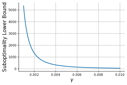
Figure 1: Consider the scalar system $X_{t+1}=aX_{t}+bU_{t}+W_{t}$. We plot a lower bound arising from Corollary 2.1 letting $V=\begin{bmatrix}0&1\end{bmatrix}^{\top}$ for the system $a=1-\gamma$, $b=\gamma$ as $\gamma$ ranges from $10^{-3}$ to $10^{-2}$ with $F=0$, $\sigma_{\tilde{u}}^{2}=1$, $\Sigma_{W}=1$. As $\gamma\to 0$ the optimally regulated system approaches marginal stability and controllability is lost. The problem of learning a controller therefore becomes challenging as $\gamma\to 0$, which is reflected by our excess cost lower bound; it approaches $\infty$. This illustrates the observation that systems which are difficult to control are also difficult to learn to control. This plot illustrates the result Corollary 2.2 in demonstrating that the global minimax excess cost is uninformative.

Our focus in obtaining the lower bound on $\mathcal{EC}^{\mathsf{lin}}_{T}(\theta,\varepsilon)$ is to gain an understanding of what system-theoretic quantities render the learning problem statistically challenging. To this end, our lower bound depends on familiar system-theoretic quantities, such as $P(\theta)$. The covariance of the state under the optimal LQR controller also appears in our analysis. Under the optimal LQR controller, the covariance of the state converges to the stationary covariance as $T\to\infty$:

$$\Sigma_{X}(\theta):=\lim_{t\to\infty}\operatorname{\textbf{E}}^{\pi_{\theta}}_{\theta}\mathopen{}\left[X_{t}X_{t}^{\top}\right]\mathclose{}=\textnormal{{dlyap}}(\mathopen{}\left(A(\theta)+B(\theta)K(\theta)\right)\mathclose{}^{\top},\Sigma_{W}).$$

1.1 Contributions

Our main contribution is the following theorem. For the formal statements, see Theorem 2.2 and Corollary 2.1.

Theorem 1.1 (Main result, Informal).

The $\varepsilon$-local minimax excess cost is lower bounded as

$$\textrm{excess cost}\geq\frac{\textrm{system-theoretic condition number}}{\textrm{\# data points}\times\textrm{signal-to-noise ratio}}.$$

In the above bound, the system-theoretic condition number depends on familiar system-theoretic quantities such as the covariance of the state under the optimal controller, and the solution to the Riccati equation. The signal-to-noise ratio depends on how easily the system is excited via both the exploratory input, and the noise. This signal-to-noise ratio may be quantified in terms of the controllability gramian of the system, as well as the exploratory input budget.

We also study several consequences of the above result by restricting attention to the setting where all system parameters are unknown, i.e. $\operatorname{\mathsf{vec}}\begin{bmatrix}A(\theta)&B(\theta)\end{bmatrix}=\theta$. In this setting, Theorem 1.1 may be reduced to $\mathcal{EC}^{\mathsf{lin}}_{T}(\theta,\varepsilon)\geq\frac{c(\theta,\varepsilon)}{NT}$, where $c(\theta,\varepsilon)$ is easily interpretable. In particular, we may reach the following conclusions:

$\bullet$ For classes of system where the operator norm of system-theoretic matrices such as the controllability gramian and the solution to the Riccati equation are constant with respect to dimension, we may take $c(\theta,\varepsilon)\propto d_{\mathsf{U}}d_{\mathsf{X}}.$ Combining results from Mania et al. (2019) and Tu et al. (2022) demonstrates that when $d_{\mathsf{U}}\leq d_{\mathsf{X}}$, the upper bound on the excess cost is also proportional to $\frac{d_{\mathsf{X}}d_{\mathsf{U}}}{NT}$. In particular, our bound is optimal in the dimension for underactuated systems when the remaining system-theoretic quantities are constant with respect to dimension.
$\bullet$ There exist classes of systems for which we may take $c(\theta,\varepsilon)\propto\exp(d_{\mathsf{X}})$. This demonstrates that the excess cost of a learned LQR controller may grow exponentially in the dimension.
$\bullet$ The lower bound grows in an interpretable manner with familiar system-theoretic quantities. In particular, we may take $c(\theta,\varepsilon)$ to grow with the eigenvalues of both the solution to the Riccati equation, $P(\theta),$ and the state covariance under the optimal controller, $\Sigma_{X}(\theta)$. This suggests that the problem of learning to control a system with a small gap from the optimal controller is data intensive when controlling the underlying system is hard.

1.2 Related Work

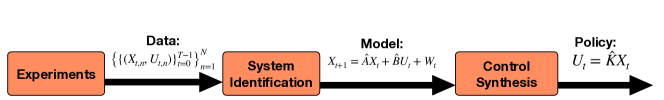
Figure 2: A classic model-based pipeline for learning a controller from data.

System Identification

System identification is often a first step in designing a controller from experimental data, and has a longstanding history. The text Ljung (1998) covers classic asymptotic results. Control oriented identification was studied in Chen and Nett (1993); Helmicki et al. (1991). Recently, there has been interest in finite sample analysis for fully-observed linear systems (Dean et al., 2019; Simchowitz et al., 2018; Faradonbeh et al., 2018; Sarkar and Rakhlin, 2019), and partially-observed linear systems (Oymak and Ozay, 2019; Sarkar et al., 2021; Simchowitz et al., 2018; Tsiamis and Pappas, 2019; Lee and Lamperski, 2020; Zheng and Li, 2020). Lower bounds for the sample complexity of system identification are presented in Jedra and Proutiere (2019); Tsiamis and Pappas (2021). For a more extensive discussion of prior work, we refer to the survey by Tsiamis et al. (2022a).

Learning Controllers Offline

Learning a controller from offline data is a familiar paradigm for control theorist and practitioners. It typically consists of system identification, followed by robust (Zhou et al., 1996) or certainty-equivalent (Simon, 1956) control design, see Figure 2. Recent work provides finite sample guarantees for such methods (Dean et al., 2019; Mania et al., 2019). Upper and lower bounds on the sample complexity of stabilization from offline data are presented in Tsiamis et al. (2022b). The RL community has a similar paradigm, known as offline RL (Levine et al., 2020). Policy gradient approaches are a model-free algorithm suitable for offline RL, and are analyzed in Fazel et al. (2018). Lower bounds on the variance of the gradient estimates in policy gradient approaches are supplied in Ziemann et al. (2022). Lower bounds for offline linear control are also studied in Wagenmaker et al. (2021) with the objective of designing optimal experiments. We instead focus on the LQR setting to understand the dependence of the excess cost on interpretable system-theoretic quantities.

Online LQR

The problem of learning the optimal LQR controller online has a rich history beginning with Åström and Wittenmark (1973). Regret minimization was introduced in Lai (1986); Lai and Wei (1986). The study of regret in online LQR was re-initiated by Abbasi-Yadkori and Szepesvári (2011), inspired by works in the RL community. Many works followed to propose algorithms which were computationally tractable (Ouyang et al., 2017; Dean et al., 2018; Abeille and Lazaric, 2018; Mania et al., 2019; Cohen et al., 2019; Faradonbeh et al., 2020; Jedra and Proutiere, 2021). Lower bounds on the regret of online LQR are presented in Simchowitz and Foster (2020); Cassel et al. (2020); Ziemann and Sandberg (2022). The results in this paper follow a similar proof to Ziemann and Sandberg (2022). The primary difference is that since our controller is designed via offline data, we may not make use of the exploration-exploitation tradeoff to upper bound the information available to the learner, as is done in Ziemann and Sandberg (2022).

2 Excess Cost Lower Bound

We now proceed to establish our lower bound. As we are interested in the worst-case excess cost from any element of $\mathcal{B}(\theta,\varepsilon)$, we make the additional assumption that $F$ stabilizes $(A(\theta^{\prime}),B(\theta^{\prime}))$ for all $\theta^{\prime}\in\mathcal{B}(\theta,\varepsilon)$. This also ensures that the optimal LQR controller exists for all points in the prior.

To obtain a lower bound on the local minimax excess cost, we lower bound the maximization over $\theta^{\prime}\in\mathcal{B}(\theta,\varepsilon)$ by an average over a distribution supported on $\mathcal{B}(\theta,\varepsilon)$. This reduces the problem to lower bounding a Bayesian complexity. Instead of fixing the parameter $\theta$, we let $\Theta$ be a random vector taking values in $\mathbb{R}^{d_{\Theta}}$ and suppose that it has prior density $\lambda$. Doing so enables the use of information theoretic tools to lower bound the complexity of estimating the parameter from data. The relaxation of the the maximization is shown in the following lemma.

Lemma 2.1.

Fix $\varepsilon>0$ and let $\lambda$ be any prior on $\mathcal{B}(\theta,\varepsilon)$. Then for any $\pi\in\Pi^{\mathsf{lin}}$ with $\pi(X_{t},\mathcal{Z})=\hat{K}(\mathcal{Z})X_{t}$,

$$\sup_{\theta^{\prime}\in\mathcal{B}(\theta)}\mathsf{EC}_{T}^{\pi}(\theta^{\prime})\geq\operatorname{\textbf{E}}\operatorname{\mathrm{tr}}\mathopen{}\left([\hat{K}(\mathcal{Z})-K(\Theta)])^{\top}\Psi(\Theta)[\hat{K}(\mathcal{Z})-K(\Theta)]\Sigma_{\Theta}^{\hat{K}(\mathcal{Z})}\right)\mathclose{},$$

where $\Sigma_{\Theta}^{\hat{K}(\mathcal{Z})}:=\frac{1}{T}\sum_{t=0}^{T-1}\operatorname{\textbf{E}}^{\pi}\mathopen{}\left[X_{t}X_{t}^{\top}|\mathcal{Z},\Theta\right]\mathclose{}$. The expectation is over the prior $\Theta\sim\lambda$, and the randomness of both the offline rollouts and the evaluation rollout. We recall the shorthand $\Psi(\Theta)=B(\Theta)^{\top}P(\Theta)B(\Theta)+R$.

Proof.

By the quadratic expression for the excess cost in (4) and the fact that the supremum over a set always exceeds the weighted average over a set, we have the following inequality:

$$\sup_{\|\theta^{\prime}-\theta\|\leq\varepsilon}\mathsf{EC}_{T}^{\pi}(\theta^{\prime})\geq\underset{\Theta\sim\lambda}{\operatorname{\textbf{E}}}R_{T}^{\pi}(\Theta)$$

$$\!\!=\!\frac{1}{T}\operatorname{\textbf{E}}\sum_{t=0}^{T-1}\operatorname{\textbf{E}}^{\pi}\mathopen{}\left[\left\|U_{t}\!-\!K(\Theta)X_{t}\right\|_{\Psi(\Theta)}^{2}|\mathcal{Z},\Theta\right]\mathclose{}$$

$$\!\!=\!\operatorname{\textbf{E}}\operatorname{\mathrm{tr}}([\hat{K}(\mathcal{Z})\!-\!K(\Theta)])^{\top}\Psi(\Theta)([\hat{K}(\mathcal{Z})-K(\Theta)]\Sigma_{\Theta}^{\hat{K}\!(\!\mathcal{Z}\!)}).$$

The second to last equality follows by the tower rule. The last equality results by substituting $U_{t}=\hat{K}(\mathcal{Z})X_{t}$, followed by the trace-cyclic property and linearity of expectation. ∎

We may treat the data from offline experimentation, $\mathcal{Z}$, as an observation of the underlying parameter $\Theta$. In particular, $\mathcal{Z}$ may be expressed as a random vector taking values in $\mathbb{R}^{NT(d_{\mathsf{X}}+d_{\mathsf{U}})}$ with conditional density $p(\cdot|\theta)$. The following Fisher information matrix and prior density concentration matrix measure estimation performance of $\Theta$ from the sample $\mathcal{Z}$ with respect to the square loss:

$$\operatorname{\mathtt{I}}_{p}(\theta) :=\int\left(\frac{\nabla_{\theta}p(z|\theta)}{p(z|\theta)}\right)\left(\frac{\nabla_{\theta}p(z|\theta)}{p(z|\theta)}\right)^{\top}p(z|\theta)dz,$$ (6)

$$\operatorname{\mathtt{J}}(\lambda) :=\int\left(\frac{\nabla_{\theta}\lambda(\theta)}{\lambda(\theta)}\right)\left(\frac{\nabla_{\theta}\lambda(\theta)}{\lambda(\theta)}\right)^{\top}\lambda(\theta)d\theta.$$ (7)

The first quantity (6) measures the information content of the sample $\mathcal{Z}$ with regards to $\Theta$. The second quantity (7) measures the concentration of the prior density $\lambda$. As the gradient operator $\nabla_{\theta}$ maps to a vector of dimension $d_{\Theta}$, both $I_{p}(\theta)$ and $J(\lambda)$ are $d_{\Theta}\times d_{\Theta}$ dimensional. See Ibragimov and Has’minskii (2013) for further details about these integrals and their existence.

As we seek lower bounds for estimating $K(\Theta)$ instead of just $\Theta$, we must account for the transformation from a quadratic loss over the error in esimating $\Theta$ to the error in estimating $K(\Theta)$, as appears in Lemma 2.1. To do so, we introduce the Van Trees’ inequality (van Trees, 2004; Bobrovsky et al., 1987). We first impose the following standard regularity conditions:

Assumption 2.1.

1. The prior $\lambda$ is smooth with compact support.

2. The conditional density of $\mathcal{Z}$ given $\Theta$, $p(z|\cdot)$, is continuously differentiable on the domain of $\lambda$ for almost every $z$.

3. The score has mean zero; $\int\left(\frac{\nabla_{\theta}p(z|\theta)}{p(z|\theta)}\right)p(z|\theta)dz=0$.

4. $\operatorname{\mathtt{J}}(\lambda)$ is finite and $\operatorname{\mathtt{I}}_{p}(\theta)$ is a continuous function of $\theta$ on the domain of $\lambda$.

5. $\operatorname{\mathsf{vec}}K$ is differentiable on the domain of $\lambda$.

The following theorem is a less general adaption from Bobrovsky et al. (1987) which suffices for our needs.

Theorem 2.1 (Van Trees Inequality).

Fix two random variables $(\mathcal{Z},\Theta)\sim p(\cdot|\cdot)\lambda(\cdot)$ and suppose Assumption 2.1 holds. Let $\mathcal{G}$ be a $\sigma(\mathcal{Z})$-measurable event. Then for any $\sigma(\mathcal{Z})$-measurable $\hat{K}$:

$$\operatorname{\textbf{E}}\left[\operatorname{\mathsf{vec}}(\hat{K}(\mathcal{Z})-K(\Theta))\operatorname{\mathsf{vec}}(\hat{K}(\mathcal{Z})-K(\Theta))^{\top}\mathbf{1}_{\mathcal{G}}\right]$$ (8)

$$\succeq\operatorname{\textbf{E}}[\operatorname{\mathsf{D}}_{\theta}\operatorname{\mathsf{vec}}K(\Theta)\mathbf{1}_{\mathcal{G}}]^{\top}\left[\operatorname{\textbf{E}}\operatorname{\mathtt{I}}_{p}(\Theta)+\operatorname{\mathtt{J}}(\lambda)\right]^{-1}\operatorname{\textbf{E}}[\operatorname{\mathsf{D}}_{\theta}\operatorname{\mathsf{vec}}K(\Theta)\mathbf{1}_{\mathcal{G}}].$$

The notation $\operatorname{\mathsf{D}}_{\theta}\operatorname{\mathsf{vec}}K(\cdot)$ above follows the standard convention for a Jacobian: it stacks the transposed gradients of each element of $\operatorname{\mathsf{vec}}K(\cdot)$ into a $d_{\mathsf{X}}d_{\mathsf{U}}\times d_{\Theta}$ dimensional matrix.

We see from Theorem 2.1 that the transformation to the error in estimating $K(\Theta)$ is accounted for by $\operatorname{\mathsf{D}}_{\theta}\operatorname{\mathsf{vec}}K(\cdot)$.

We now massage the lower bound in Lemma 2.1 to a form compatible with Theorem 2.1. Doing so requires us to express the lower bound as a quadratic form conditioned on some $\sigma(\mathcal{Z})$-measureable event $\mathcal{G}$. We therefore select an event $\mathcal{G}$ for which we may uniformly lower bound the quantities $\Psi(\Theta)$ and $\Sigma_{\Theta}^{\hat{K}(\mathcal{Z})}$. To this end, we define positive definite matrices $\Psi_{\theta,\varepsilon}$ and $\Sigma_{\theta,\varepsilon}$ that satisfy

$$\Psi(\theta^{\prime}) \succeq\Psi_{\theta,\varepsilon}\textrm{ and }\frac{1}{2}\Sigma_{X}(\theta^{\prime})\succeq\Sigma_{\theta,\varepsilon}\quad\forall\theta^{\prime}\in\mathcal{B}(\theta,\varepsilon).$$ (9)

The matrix $\Psi_{\theta,\varepsilon}$ will serve to uniformly lower bound $\Psi(\Theta)$. When the learned controller is close to the optimal controller, the covariance of the state under the learned controller will be close to the covariance of the state under the optimal controller, which is in turn lower bounded in terms of $\Sigma_{\theta,\varepsilon}$. In particular, if $\left\|\hat{K}(\mathcal{Z})-K(\Theta)\right\|$ is sufficiently small, we can argue that $\Sigma_{\Theta}^{\hat{K}(\mathcal{Z})}\succeq\frac{1}{2}\Sigma_{X}(\Theta)\succeq\Sigma_{\theta,\varepsilon}$. The aforementioned condition on $\left\|\hat{K}(\mathcal{Z})-K(\Theta)\right\|$ will hold only if there is a large amount of data available to fit $\hat{K}(\mathcal{Z})$. To achieve a bound that holds in the low data regime, we observe that the state covariance under the learned controller is always lower bounded by the noise covariance: $\Sigma_{\Theta}^{\mathcal{Z}}\succeq\Sigma_{W}$. For this reason, the subsequent results will be presented in two parts: one in which we condition on an event where $\left\|\hat{K}(\mathcal{Z})-K(\theta)\right\|$ is small, and one that holds generally. To present these results concisely, the positive definite matrix $\Gamma_{\theta,\varepsilon}$ is used to denote either $\Sigma_{W}$ or $\Sigma_{\theta,\varepsilon}$. The Kronecker product of these lower bounds arises frequently, motivating the shorthand

$$\Xi_{\theta,\varepsilon}:=\Gamma_{\theta,\varepsilon}\otimes\Psi_{\theta,\varepsilon}.$$ (10)

Lemma 2.2 (Application of Van Trees’ Inequality).

For any smooth prior $\lambda$ on $\mathcal{B}(\theta,\varepsilon)$ and any $\pi\in\Pi^{\mathsf{lin}}$ with $\pi(X_{t},\mathcal{Z})=\hat{K}(\mathcal{Z})X_{t}$,

$$\sup_{\theta^{\prime}\in\mathcal{B}(\theta,\varepsilon)}\mathsf{EC}_{T}^{\pi}(\theta^{\prime})\geq\frac{\operatorname{\mathrm{tr}}\left(\Xi_{\theta,\varepsilon}\operatorname{\textbf{E}}[\operatorname{\mathsf{D}}_{\theta}\operatorname{\mathsf{vec}}K(\Theta)\mathbf{1}_{\mathcal{G}}]\operatorname{\textbf{E}}[\operatorname{\mathsf{D}}_{\theta}\operatorname{\mathsf{vec}}K(\Theta)\mathbf{1}_{\mathcal{G}}]^{\top}\right)}{\left\|\operatorname{\textbf{E}}\operatorname{\mathtt{I}}_{p}(\Theta)+\operatorname{\mathtt{J}}(\lambda)\right\|},$$ (11)

where either:

$1)$ $\Gamma_{\theta,\varepsilon}=\Sigma_{W}$ and $\mathcal{G}=\Omega$, or
$2)$ $\Gamma_{\theta,\varepsilon}=\Sigma_{\theta,\varepsilon}$ and $\mathcal{G}=\mathcal{E}$, if $\displaystyle T\geq\sup_{\theta^{\prime}\in\mathcal{B}(\theta,\varepsilon)}\frac{16\left\|\Sigma_{X}(\theta^{\prime})\right\|}{\lambda_{\min}(\Sigma_{X}(\theta^{\prime}))}$.

The event $\Omega$ is the entire sample space, i.e. $\operatorname{\mathbb{P}}\mathopen{}\left[\Omega\right]\mathclose{}=1$, and

$$\mathcal{E} =\mathopen{}\left\{\sup_{\theta^{\prime}\in\mathcal{B}(\theta,\varepsilon)}\left\|\hat{K}(\mathcal{Z})-K(\theta^{\prime})\right\|\leq\alpha\right\}\mathclose{}$$

$$\alpha =\inf_{\theta^{\prime}\in\mathcal{B}(\theta,\varepsilon)}\min\mathopen{}\left\{\frac{\left\|A_{cl}(\theta^{\prime})\right\|}{\left\|B(\theta^{\prime})\right\|},\frac{\lambda_{\min}(\Sigma_{X}(\theta^{\prime}))/24}{\left\|A_{cl}(\theta^{\prime})\right\|\left\|B(\theta^{\prime})\right\|\mathcal{J}(A_{cl}(\theta^{\prime}))\left\|\Sigma_{X}(\theta^{\prime})\right\|}\right\}\mathclose{}.$$

Here, $A_{cl}(\theta)=A(\theta)+B(\theta)K(\theta)$ and $\mathcal{J}(A_{cl}(\theta))=\sum_{t=0}^{\infty}\left\|A_{cl}(\theta)^{t}\right\|^{2}$.

Proof.

We always have that $\Sigma_{\hat{K}(\mathcal{Z})}\succeq\Sigma_{W}$. Lemma A.2 shows that if $T\geq\frac{16\left\|\Sigma_{X}(\Theta)\right\|^{2}}{\lambda_{\min}(\Sigma_{X}(\Theta))}$, then under event $\mathcal{E}$, we have $\left\|\Sigma_{X}(\Theta)^{-1/2}\Sigma_{\Theta}^{\hat{K}(\mathcal{Z})}\Sigma_{X}(\Theta)^{-1/2}-I\right\|\leq\frac{1}{2}$. This in turn implies that $\Sigma_{\Theta}^{\hat{K}(\mathcal{Z})}\succeq\Sigma_{\theta,\varepsilon}\mathbf{1}_{\mathcal{E}}$.

With this fact in hand, we may replace $\Psi(\Theta)$ in the lower bound from Lemma 2.1 by $\Psi_{\theta,\varepsilon}$, and $\Sigma_{\Theta}^{\hat{K}(\mathcal{Z})}$ by $\Gamma_{\theta,\varepsilon}\mathbf{1}_{\mathcal{G}}$, where $(\Gamma_{\theta,\varepsilon},\mathcal{G})$ can only be set as $(\Sigma_{\theta,\varepsilon},\mathcal{E})$ if $T$ is sufficiently large. Then

$$\sup_{\theta^{\prime}\in\mathcal{B}(\theta,\varepsilon)}\mathsf{EC}_{T}^{\pi}(\theta^{\prime})\geq\operatorname{\textbf{E}}\operatorname{\mathrm{tr}}([\hat{K}(\mathcal{Z})-K(\Theta)])^{\top}\Psi_{\theta,\varepsilon}([\hat{K}(\mathcal{Z})-K(\Theta)]\Gamma_{\theta,\varepsilon})\mathbf{1}_{\mathcal{G}}$$

$$=\operatorname{\textbf{E}}\operatorname{\mathrm{tr}}([\tilde{K}(\mathcal{Z})-\sqrt{\Psi_{\theta,\varepsilon}}K(\Theta)\sqrt{\Gamma_{\theta,\varepsilon}}])^{\top}[\tilde{K}(\mathcal{Z})-\sqrt{\Psi_{\theta,\varepsilon}}K(\Theta)\sqrt{\Gamma_{\theta,\varepsilon}}])\mathbf{1}_{\mathcal{G}}$$

$$=\operatorname{\textbf{E}}\operatorname{\mathrm{tr}}\big{(}[\operatorname{\mathsf{vec}}\tilde{K}(\mathcal{Z})-\operatorname{\mathsf{vec}}\sqrt{\Psi_{\theta,\varepsilon}}K(\Theta)\sqrt{\Gamma_{\theta,\varepsilon}}]\cdot[\operatorname{\mathsf{vec}}\tilde{K}(\mathcal{Z})-\operatorname{\mathsf{vec}}\sqrt{\Psi_{\theta,\varepsilon}}K(\Theta)\sqrt{\Gamma_{\theta,\varepsilon}}]\big{)}^{\top}\mathbf{1}_{\mathcal{G}},$$

where $\tilde{K}(\mathcal{Z})=\sqrt{\Psi_{\theta,\varepsilon}}\hat{K}(\mathcal{Z})\sqrt{\Gamma_{\theta,\varepsilon}}$. We now invoke the Van Trees’ inequality, Theorem 2.1:

$$\sup_{\theta^{\prime}\in\mathcal{B}(\theta,\varepsilon)}\mathsf{EC}_{T}^{\pi}(\theta^{\prime})\!\geq\!\operatorname{\mathrm{tr}}\mathopen{}\left(\!\operatorname{\textbf{E}}[\operatorname{\mathsf{D}}_{\theta}\operatorname{\mathsf{vec}}\sqrt{\Psi_{\theta,\varepsilon}}K(\Theta)\sqrt{\Gamma_{\theta,\varepsilon}}\mathbf{1}_{\mathcal{G}}]\left[\operatorname{\textbf{E}}\operatorname{\mathtt{I}}_{p}(\Theta)\!+\!\operatorname{\mathtt{J}}(\lambda)\right]^{-1}\!\operatorname{\textbf{E}}[\operatorname{\mathsf{D}}_{\theta}\operatorname{\mathsf{vec}}\sqrt{\Psi_{\theta,\varepsilon}}K(\Theta)\sqrt{\Gamma_{\theta,\varepsilon}}\mathbf{1}_{\mathcal{G}}]^{\top}\!\right)\mathclose{}$$

$$\!=\!\operatorname{\mathrm{tr}}\mathopen{}\left(\!\operatorname{\textbf{E}}[(\sqrt{\Gamma_{\theta,\varepsilon}}\!\otimes\!\sqrt{\Psi_{\theta,\varepsilon}})\operatorname{\mathsf{D}}_{\theta}\operatorname{\mathsf{vec}}K(\Theta)\mathbf{1}_{\mathcal{G}}]\left[\operatorname{\textbf{E}}\operatorname{\mathtt{I}}_{p}(\Theta)+\operatorname{\mathtt{J}}(\lambda)\right]^{-1}\operatorname{\textbf{E}}[(\sqrt{\Gamma_{\theta,\varepsilon}}\!\otimes\!\sqrt{\Psi_{\theta,\varepsilon}})\operatorname{\mathsf{D}}_{\theta}\operatorname{\mathsf{vec}}K(\Theta)\mathbf{1}_{\mathcal{G}}]^{\top}\!\right)\mathclose{},$$

where we used that $\operatorname{\mathsf{vec}}\sqrt{\Psi_{\theta,\varepsilon}}K(\Theta)\sqrt{\Gamma_{\theta,\varepsilon}}=(\sqrt{\Gamma_{\theta,\varepsilon}}\otimes\sqrt{\Psi_{\theta,\varepsilon}})\operatorname{\mathsf{vec}}K(\Theta)$ in the last line.

We conclude by applying the trace cyclic property, and extracting the minimum eigenvalue of $[\operatorname{\textbf{E}}_{\Theta}I_{p}(\theta)+J(\lambda)]^{-1}$.

∎

Lemma 2.2 may be interpreted according to the following intuition. To design a controller that attains low cost, it is essential to distinguish between two nearby instances of the underlying parameter, $\theta$ and $\theta^{\prime}$, from the experimental data, $\mathcal{Z}$. The Fisher Information term on the denominator of the bound in Lemma 2.2 captures the ease with which we can distinguish between $\theta$ and an infinitesimally perturbed $\theta^{\prime}$ from the collected data $\mathcal{Z}$, and can be thought of as a signal-to-noise ratio. The derivative of the controller appearing on the numerator of the bound in Lemma 2.2 is a change of variables term that accounts for the extent to which infinitesimal perturbations of the underlying parameter impact the optimal controller gain. Sensitive perturbations are those which are difficult to detect from the collected data, yet lead to a large change in the controller gain. Such perturbations dictate the statistical hardness of learning a LQR controller. Motivated by this fact, we can select particularly sensitive perturbation directions of the underlying parameter which emphasize the hardness of the problem. To do so, we restrict the support of the prior $\lambda$ to a lower dimensional subspace. Before presenting this result, it will be useful to see the expression for Fisher information matrix from this experimental setup. It can be shown via the chain rule of Fisher Information that

$$I_{p}(\theta)=\operatorname{\textbf{E}}_{\theta}\sum_{n=1}^{N}\sum_{t=0}^{T-1}\operatorname{\mathsf{D}}_{\theta}\operatorname{\mathsf{vec}}\begin{bmatrix}A(\theta)&B(\theta)\end{bmatrix}^{\top}[Z_{t,n}Z_{t,n}^{\top}\otimes\Sigma_{W}^{-1}]\operatorname{\mathsf{D}}_{\theta}\operatorname{\mathsf{vec}}\begin{bmatrix}A(\theta)&B(\theta)\end{bmatrix},$$ (12)

where $Z_{t,n}=\begin{bmatrix}X_{t,n}\\ U_{t,n}\end{bmatrix}$. See, for instance, Lemma 3.1 of Ziemann and Sandberg (2022). With this in hand, the following Lemma provides a restriction to lower dimensional priors, which allows us to understand how poor conditioning of the information matrix along any particular parameter perturbation direction pushes through to a challenge in estimating the optimal controller.

Lemma 2.3.

Consider any matrix $V\in\mathbb{R}^{d_{\Theta}\times k}$ with $k\leq d_{\Theta}$ which has orthonormal columns. For any smooth prior $\lambda$ over $\mathopen{}\left\{\theta+V\tilde{\theta}:\left\|\tilde{\theta}\right\|\leq\varepsilon\right\}\mathclose{}$, and any $\pi\in\Pi^{\mathsf{lin}}$ with $\pi(X_{t},\mathcal{Z})=\hat{K}(\mathcal{Z})X_{t}$,

$$\sup_{\theta^{\prime}\in\mathcal{B}(\theta,\varepsilon)}\mathsf{EC}_{T}^{\pi}(\theta^{\prime})\geq\frac{\operatorname{\mathrm{tr}}\left(\Xi_{\theta,\varepsilon}\operatorname{\textbf{E}}[\operatorname{\mathsf{D}}_{\theta}\operatorname{\mathsf{vec}}K(\Theta)V\mathbf{1}_{\mathcal{G}}]\operatorname{\textbf{E}}[\operatorname{\mathsf{D}}_{\theta}\operatorname{\mathsf{vec}}K(\Theta)V\mathbf{1}_{\mathcal{G}}]^{\top}\right)}{\left\|V^{\top}\mathopen{}\left(\operatorname{\textbf{E}}\operatorname{\mathtt{I}}_{p}(\Theta)+\operatorname{\mathtt{J}}(\lambda)\right)\mathclose{}V\right\|},$$

where $\Xi_{\theta,\varepsilon}$ is defined in (10) and $\mathcal{G}$ is defined in Lemma 2.2.

Proof.

We may write $\Theta=\theta+V\tilde{\Theta}$, where $\tilde{\Theta}\sim\tilde{\lambda}$, and $\tilde{\lambda}$ is a smooth prior on $\mathopen{}\left\{\tilde{\theta}\in\mathbb{R}^{k}:\left\|\tilde{\theta}\right\|\leq\epsilon\right\}\mathclose{}$. Defining $\tilde{A}(\tilde{\theta}):=A(\theta+V\tilde{\theta})$, $\tilde{B}(\tilde{\theta}):=B(\theta+V\tilde{\theta})$, and $\tilde{K}(\tilde{\theta}):=K(\theta+V\tilde{\theta})$, we may instantiate the bound in Lemma 2.2 over the lower dimensional parameter $\tilde{\theta}$. We have that the Jacobian of the contoller becomes $\operatorname{\mathsf{D}}_{\tilde{\theta}}\operatorname{\mathsf{vec}}\tilde{K}(\tilde{\Theta})=\operatorname{\mathsf{D}}_{\theta}\operatorname{\mathsf{vec}}K(\Theta)V.$ Similarly, the Jacobian arising in the Fisher information may be written $D_{\tilde{\theta}}\operatorname{\mathsf{vec}}\begin{bmatrix}\tilde{A}(\tilde{\Theta})&\tilde{B}(\tilde{\Theta})\end{bmatrix}=D_{\theta}\operatorname{\mathsf{vec}}\begin{bmatrix}A(\Theta)&B(\Theta)\end{bmatrix}V$. Lastly, the prior density of the lower dimensional parameter satisfies $\tilde{J}(\tilde{\lambda})=V^{\top}J(\lambda)V$. Then under this prior, the lower bound in Lemma 2.2 becomes that in the lemma statement. ∎

In the above lemma, the columns of $V$ may be interpreted as perturbation directions of the system parameters.

We now upper bound the denominator arising in the above bound. In particular, we show how to bound the Fisher Information in any particular perturbation direction.

Lemma 2.4.

For any matrix $V\in\mathbb{R}^{d_{\Theta}\times k}$ with orthonormal columns,

$$\left\|V^{\top}\operatorname{\textbf{E}}\mathopen{}\left[I_{p}(\Theta)\right]\mathclose{}V\right\| \leq TN\bar{L},$$

where $\bar{L}=\sup_{\theta^{\prime}\in\mathcal{B}(\theta,\varepsilon)}L(\theta^{\prime})$ and

$$L(\theta^{\prime})=\sup_{w\in\textbf{span}(V),\left\|w\right\|\leq 1}\frac{4}{\lambda_{\min}(\Sigma_{W})}$$ (13)

$$\cdot\Bigg{(}\nu_{1}(w)\bigg{(}\left\|\textnormal{{dlyap}}\mathopen{}\left((A(\theta^{\prime})+B(\theta^{\prime})F)^{\top},\Sigma_{W}\right)\mathclose{}\right\|$$

$$\!+\!\sigma_{\tilde{u}}^{2}\mathopen{}\left(\sum_{t=0}^{\infty}\left\|(A(\theta^{\prime})\!+\!B(\theta^{\prime})F)^{t}B\right\|\right)\mathclose{}^{2}\Bigg{)}\!+\!2\sigma_{\tilde{u}}^{2}\nu_{2}(w)\bigg{)}.$$

Here, $\nu_{1}(w)=\left\|D_{\theta}\operatorname{\mathsf{vec}}A(\theta^{\prime})w\right\|^{2}+2\left\|D_{\theta}\operatorname{\mathsf{vec}}B(\theta^{\prime})w\right\|^{2}\left\|F\right\|^{2}$ and $\nu_{2}(w)=\left\|D_{\theta}\operatorname{\mathsf{vec}}B(\theta^{\prime})w\right\|^{2}$ are change of coordinate terms that quantify the impact of the perturbation direction on the information upper bound. We recall that $\sigma_{\tilde{u}}^{2}$ is the average exploratory input energy.

The quantity $\textnormal{{dlyap}}((A(\theta^{\prime})+B(\theta^{\prime})F)^{\top},\Sigma_{W})$, in the above bound may be interpreted as either the steady state covariance during exploration in the absence of exploratory inputs, or the controllability gramian from the noise to the state. The quantity $\sum_{t=0}^{\infty}\left\|(A(\theta^{\prime})+B(\theta^{\prime})F)^{t}B(\theta^{\prime})\right\|$ bounds the $\mathcal{H}_{\infty}$ norm of the closed-loop system during offline experimentation. Therefore, $\sigma_{\tilde{u}}^{2}\mathopen{}\left(\sum_{t=0}^{\infty}\left\|(A(\theta^{\prime})+B(\theta^{\prime})F)^{t}B(\theta^{\prime})\right\|\right)\mathclose{}^{2}$ upper bounds the impact of exploratory input on the state during offline experimentation. The proof of the above lemma applies repeated use of the triangle inequality, submultiplicativity, the Cauchy-Schwarz inequality. See Section A.1 for proof details.

We now present our first main result: a non-asymptotic lower bound on the local minimax excess cost. As with Lemma 2.2, it is presented in two components: one that holds generally, and another that requires enough data such that any sufficiently good policy $\pi\in\Pi_{\mathsf{lin}}$ outputs a feedback controller $\hat{K}(\mathcal{Z})$ which is near optimal with high probability. Consequently, the burn-in times are larger for the second result, and the size of the prior, $\varepsilon$, is required to be small. We drop the dependence of $A$, $B$, $P$, $\Psi$, $K$, and $\Sigma_{X}$ on $\theta$ when the argument is clear from context.

Theorem 2.2.

Consider any matrix $V\in\mathbb{R}^{d_{\Theta}\times k}$ with $k\leq d_{\Theta}$ which has orthonormal columns. Let

$$G =\inf_{\theta^{{}^{\prime}},\tilde{\theta}\in\mathcal{B}(\theta,\varepsilon)}\operatorname{\mathrm{tr}}\bigg{(}\Xi_{\theta,\varepsilon}\operatorname{\mathsf{D}}_{\theta}\operatorname{\mathsf{vec}}K(\theta^{\prime})V\mathopen{}\left(\operatorname{\mathsf{D}}_{\theta}\operatorname{\mathsf{vec}}K(\tilde{\theta})V\right)\mathclose{}^{\top}\bigg{)},$$

and $\bar{L}$ be as in Lemma 2.4. Also let $\Xi_{\theta,\varepsilon}$ be as defined in (10). Then for any smooth prior $\lambda$ over $\mathopen{}\left\{\theta+V\tilde{\theta}:\left\|\tilde{\theta}\right\|\leq\varepsilon\right\}\mathclose{}$,

$$\mathcal{EC}^{\mathsf{lin}}_{T}(\theta,\varepsilon) \geq\frac{G}{8NT\bar{L}}$$ (14)

is satisfied for

$1)$ $\Gamma_{\theta,\varepsilon}=\Sigma_{W}$ if $TN\geq\frac{\left\|J(\lambda)\right\|}{\bar{L}}$.
$2)$ $\Gamma_{\theta,\varepsilon}=\Sigma_{\theta,\varepsilon}$ if $T\geq\sup_{\theta^{\prime}\in\mathcal{B}(\theta,\varepsilon)}\frac{16\left\|\Sigma_{X}(\theta^{\prime})\right\|^{2}}{\lambda_{\min}(\Sigma_{X}(\theta^{\prime}))}$, $TN\geq\frac{1}{\bar{L}}{\max\mathopen{}\left\{\left\|J(\lambda)\right\|,\frac{G}{\lambda_{\min}(\Sigma_{W})\lambda_{\min}(R)\alpha^{2}}\right\}\mathclose{}}$, and $\varepsilon\leq\min\mathopen{}\left\{\frac{\alpha}{2c_{1}},c_{2}\right\}\mathclose{}$, where

$$c_{1} =84\Phi^{9}\tau(A_{cl})$$

$$c_{2} =\frac{1}{10\tau(A_{cl})c_{1}}\min\mathopen{}\left\{(1+\left\|A_{cl}\right\|)^{-2},(1+\left\|P\right\|)^{-1}\right\}\mathclose{}$$

$$\Phi =(1+\max\mathopen{}\left\{\left\|A\right\|,\left\|B\right\|,\left\|P\right\|,\left\|K\right\|,\left\|R^{-1}\right\|\right\}\mathclose{})$$

$$\tau(A_{cl}) =\mathopen{}\left(\sup_{k\geq 0}\mathopen{}\left\{\left\|A_{cl}^{k}\right\|\rho(A_{cl})^{-k}\right\}\mathclose{}\right)\mathclose{}^{2}/(1-\rho(A_{cl})^{2}).$$

Proof.

We must show that for all $\pi\in\Pi^{\mathsf{lin}}$, $\sup_{\theta^{\prime}\in\mathcal{B}(\theta,\varepsilon)}\mathsf{EC}_{T}^{\pi}(\theta^{\prime})\geq\frac{G}{8NT\bar{L}}$. Suppose that for some $\pi\in\Pi^{\mathsf{lin}}$, $\sup_{\theta^{\prime}\in\mathcal{B}(\theta,\varepsilon)}\mathsf{EC}_{T}^{\pi}(\theta^{\prime})\leq\frac{G}{8NT\bar{L}}$. We have by Lemma 2.3 that

$$\sup_{\theta^{\prime}\in\mathcal{B}(\theta,\varepsilon)}\mathsf{EC}_{T}^{\pi}(\theta^{\prime})\geq\frac{\operatorname{\mathrm{tr}}\left(\Xi_{\theta,\varepsilon}\operatorname{\textbf{E}}[\operatorname{\mathsf{D}}_{\theta}\operatorname{\mathsf{vec}}K(\Theta)V\mathbf{1}_{\mathcal{G}}]\operatorname{\textbf{E}}[\operatorname{\mathsf{D}}_{\theta}\operatorname{\mathsf{vec}}K(\Theta)V\mathbf{1}_{\mathcal{G}}]^{\top}\right)}{\left\|V^{\top}\mathopen{}\left(\operatorname{\textbf{E}}\operatorname{\mathtt{I}}_{p}(\Theta)+\operatorname{\mathtt{J}}(\lambda)\right)\mathclose{}V\right\|}.$$ (15)

The burn-in requirement $TN\geq\frac{\left\|J(\lambda)\right\|}{\bar{L}}$ enables upper bounding $\left\|V^{\top}J(\lambda)V\right\|$ by $TN\bar{L}$. Lemma 2.4 then allows us to upper bound the denominator in (15) by $2TN\bar{L}$.

To remove the indicators from the lower bound, we take an infimum over $\tilde{\theta},\theta^{\prime}\in\mathcal{B}(\theta,\varepsilon)$ to lower bound the numerator in (15) by $\mathbf{P}[\mathcal{G}]^{2}G$. For case 1, we immediately have $\mathbf{P}[\mathcal{G}]^{2}=\mathbf{P}[\Omega]^{2}=1$. For case 2, we may leverage the assumptions that the prior is small and that the burn-in time is satisfied to show that $\mathbf{P}[\mathcal{G}]^{2}=\mathbf{P}[\mathcal{E}]^{2}\geq\frac{1}{4}$. See Section A.2 for more details. This in turn implies that

$$\sup_{\theta^{\prime}\in\mathcal{B}(\theta,\varepsilon)}\mathsf{EC}_{T}^{\pi}(\theta^{\prime})\geq\frac{G}{8TN\bar{L}}.$$

Therefore, for all $\pi\in\Pi^{\mathsf{lin}}$, the above lower bound is satisfied. This implies that

$$\mathcal{EC}^{\mathsf{lin}}_{T}(\theta,\varepsilon)=\inf_{\pi\in\Pi^{\mathsf{lin}}}\sup_{\theta^{\prime}\in\mathcal{B}(\theta,\varepsilon)}\mathsf{EC}_{T}^{\pi}(\theta^{\prime})\geq\frac{G}{8TN\bar{L}}.$$

∎

The above result holds non-asymptotically. It will be helpful to present the result asymptotically, as the number of experiments tends to $\infty$ for an understanding of the dependence on control-theoretic quantities.

Corollary 2.1.

For any $\alpha\in(0,1/2)$ and any matrix $V\in\mathbb{R}^{d_{\Theta}\times k}$ with $k\leq d_{\Theta}$ which has orthonormal columns, we have that

$$\liminf_{N\to\infty}\sup_{\theta^{\prime}\in\mathcal{B}(\theta,N^{-\alpha})}N\mathsf{EC}_{T}^{\pi}(\theta^{\prime})\geq\frac{G}{8TL(\theta)},$$

holds always for $\Gamma=\Sigma_{W}$ and for $\Gamma=\frac{1}{2}\Sigma_{X}$ if $T\geq\frac{16\left\|\Sigma_{X}\right\|^{2}}{\lambda_{\min}(\Sigma_{X})}$, where $L$ is as in Lemma 2.4 and

$$G =\operatorname{\mathrm{tr}}\left((\Gamma\otimes\Psi)\operatorname{\mathsf{D}}_{\theta}\operatorname{\mathsf{vec}}K(\theta)V\mathopen{}\left(\operatorname{\mathsf{D}}_{\theta}\operatorname{\mathsf{vec}}K(\theta)V\right)\mathclose{}^{\top}\right).$$

Proof.

The burn-in requirements in Theorem 2.2 are satisfied asymptotically, see Section A.3 for more details. ∎

Using a similar argument to the derivations above, it can be shown that the global minimax complexity is infinite.

Corollary 2.2.

The global minimax excess cost is infinite for the class of scalar systems of the form:

$$X_{t+1}=aX_{t}+bU_{t}+W_{t},$$

with $\theta=\begin{bmatrix}a&b\end{bmatrix}^{\top}$, and $Q=R=\Sigma_{W}=\sigma_{\tilde{u}}^{2}=1$. More precisely, for the class of stable scalar systems with the offline exploration policy $F=0$, we have

$$\liminf_{N\to\infty}\sup_{a,b:{\left|a\right|}<1}N\mathsf{EC}_{T}^{\pi}(a,b)=\infty.$$

Proof.

We argue as in the proof of Corollary 2.1 with $V=\begin{bmatrix}0&1\end{bmatrix}^{\top}$. In this perturbation direction, the lower bound evaluates to $\frac{1}{T}\frac{b^{2}P+1}{32}\frac{\partial K}{\partial b}(a,b)^{2}$. Considering $a=1-\gamma$ and $b=\gamma$ for $0<\gamma<1$ and taking the limit as $\gamma\to 0$ results in the lower bound of $\infty$. For more details, see Section A.4. ∎

3 Consequences of the Lower Bound

In this section, we examine cases where the bound in Corollary 2.1 has interpretable dependence upon system properties. To do so, we restrict attention to the setting where all system parameters are unknown, i.e. $\operatorname{\mathsf{vec}}\begin{bmatrix}A(\theta)&B(\theta)\end{bmatrix}=\theta$. In this setting, the quantity $\operatorname{\mathsf{D}}_{\theta}\operatorname{\mathsf{vec}}\begin{bmatrix}A(\theta)&B(\theta)\end{bmatrix}$ arising in the bounds from the previous section is the identity matrix.

The derivative of the controller multiplied by a matrix with orthonormal columns, $\operatorname{\mathsf{D}}_{\theta}\operatorname{\mathsf{vec}}K(\theta)V$, arises in the bounds from the previous section. In this section, this quantity is expressed in terms of the directional derivative of the controller in some direction $v$, denoted $d_{v}K(\theta)$. In particular, we represent the columns of $V$ as $v=\operatorname{\mathsf{vec}}\begin{bmatrix}\Delta_{A}&\Delta_{B}\end{bmatrix}$ for arbitrary perturbations $\Delta_{A}$ of $A$ and $\Delta_{B}$ of $B$ which satisfy $\left\|\begin{bmatrix}\Delta_{A}&\Delta_{B}\end{bmatrix}\right\|_{F}=1$. The corresponding change in the closed-loop state matrix is denoted $\Delta_{A_{cl}}=\Delta_{A}+\Delta_{B}K$. Then the directional derivative of the controller is shown in Lemma B.1 of Simchowitz and Foster (2020) to be

$$d_{v}K(\theta)\!=\!-\!\Psi^{-1}(\Delta_{B}^{\top}PA_{cl}\!+\!B^{\top}P\Delta_{A_{cl}}\!+\!B^{\top}P^{\prime}A_{cl}),$$ (16)

where $P^{\prime}=\texttt{dlyap}(A_{cl},A_{cl}^{\top}P\Delta_{A_{cl}}+\Delta_{A_{cl}}^{\top}PA_{cl})$. The subsequent sections study the bound from Corollary 2.1 under various perturbations $\begin{bmatrix}\Delta_{A}&\Delta_{B}\end{bmatrix}$. Proofs are deferred to Appendix B.

3.1 Dimensional dependence

In the setting of online LQR for an unknown system, recent works (Simchowitz and Foster, 2020; Ziemann and Sandberg, 2022) obtaining lower bounds on the regret have used perturbation directions which cause tension between identification and control (Polderman, 1986). In particular, they considered the set of perturbation directions

$$\bm{\Delta}=\mathopen{}\left\{\operatorname{\mathsf{vec}}\begin{bmatrix}-\Delta K&\Delta\end{bmatrix}\bigg{|}\Delta\in\mathbb{R}^{d_{\mathsf{X}}\times d_{\mathsf{U}}},\left\|\begin{bmatrix}-\Delta K&\Delta\end{bmatrix}\right\|_{F}=1\right\}\mathclose{}.$$ (17)

For all such perturbations, $\Delta_{A_{cl}}=0$, making it impossible to distinguish between the true parameters and the perturbed parameters online without sufficient exploratory input noise.

While the tension between identification and control is no longer present in the offline setting, this set of perturbation directions retains the benefit that the directional derivative in (16) is easy to work with. In particular for any $v=\operatorname{\mathsf{vec}}\begin{bmatrix}-\Delta K&\Delta\end{bmatrix}\in\bm{\Delta}$,

$$d_{v}K(\theta)=-\Psi^{-1}\Delta^{\top}PA_{cl}.$$ (18)

As the matrices $\Delta$ parametrizing the set $\bm{\Delta}$ are $d_{\mathsf{X}}\times d_{\mathsf{U}}$ dimensional, we may stack $d_{\mathsf{X}}d_{\mathsf{U}}$ orthogonal vectors $v_{i}$ belonging $\bm{\Delta}$ into a matrix $V=\begin{bmatrix}v_{1}&\dots&v_{d_{\mathsf{X}}d_{\mathsf{U}}}\end{bmatrix}$. This allows us to present a lower bound which demonstrates the dependence of the offline LQR problem upon the system dimensions $d_{\mathsf{X}}$ and $d_{\mathsf{U}}$.

Proposition 3.1.

Suppose that $T\geq\frac{16\left\|\Sigma_{X}\right\|^{2}}{\lambda_{\min}(\Sigma_{X})}$. Then for $\alpha\in(0,1/2)$,

$$\liminf_{N\to\infty}\sup_{\theta^{\prime}\in\mathcal{B}(\theta,N^{-\alpha})}N\mathsf{EC}_{T}^{\pi}(\theta^{\prime})\geq\frac{d_{\mathsf{X}}d_{\mathsf{U}}\lambda_{\min}(\Sigma_{X}-\Sigma_{W})\lambda_{\min}(P)^{2}}{16T\left\|\Psi\right\|\left\|\begin{bmatrix}-K&I\end{bmatrix}\right\|^{2}\tilde{L}}$$

where $\tilde{L}$ is given by $L(\theta)$ as in (LABEL:eq:_info_bound_L) by replacing $\nu_{1}$ with $1$ and $\nu_{2}$ with $1+2\left\|F\right\|^{2}$.

In addition to the system dimensions, we can interpret the remaining system-theoretic parameters. Note that $\tilde{L}$ bounds the information available from the offline experimentation. It depends on the norm of the controllability gramian from noise to the state, as well as $\sigma_{\tilde{u}}^{2}\mathopen{}\left(\sum_{t=0}^{\infty}\left\|(A+BF)^{t}B\right\|\right)\mathclose{}^{2}$, which bounds the impact of the exploratory input on the state. The $\Psi$ in the denominator of the above bound may scale as $\lambda_{\max}(P)$, and therefore effectively cancels a $\lambda_{\min}(P)$ in the numerator for well-conditioned problems. This leaves a single $\lambda_{\min}(P)$ in the numerator. As $x^{\top}Px$ is the optimal objective value of the noiseless LQR problem starting from initial state $x$, the appearance of $\lambda_{\min}(P)$ in the bound captures the fact that as the system becomes harder to control, it also becomes harder to learn to control. Lastly, the variance term $\lambda_{\min}(\Sigma_{X}-\Sigma_{W})$ implies that the excess cost is large when the optimal closed-loop system has a large state covariance relative to the process noise covariance.

Remark 3.1.

The dimensional dependence $d_{\mathsf{X}}d_{\mathsf{U}}$ in the above bound is optimal up to constant factors when $d_{\mathsf{U}}\leq d_{\mathsf{X}}$. To see that this is so, observe that Theorem 2 of Mania et al. (2019) demonstrates an upper bound on the excess cost that scales as $d_{\mathsf{U}}\varepsilon^{2}$, where $\varepsilon^{2}$ bounds the system identification error, $\max\mathopen{}\left\{\left\|\hat{A}-A\right\|^{2},\left\|\hat{B}-B\right\|^{2}\right\}\mathclose{}$. A consequence of Theorem 5.4 in Tu et al. (2022) is that if we apply exploratory inputs which are generated from a Gaussian distribution with mean zero and covariance $\sigma_{\tilde{u}}^{2}I$, then the upper bound on the system identification error scales as $\frac{d_{\mathsf{X}}+d_{\mathsf{U}}}{NT}$. In particular, as long as number of offline trajectories $N$ exceeds $cd_{\mathsf{X}}$, for some universal constant $c$, then $\max\mathopen{}\left\{\left\|\hat{A}-A\right\|^{2},\left\|\hat{B}-B\right\|^{2}\right\}\mathclose{}\lesssim\left\|\Sigma_{W}\right\|\frac{d_{\mathsf{X}}+d_{\mathsf{U}}}{NT\lambda_{\min}(\textrm{controllability gramian})}$. Consequently, the upper bound on the excess cost scales with $\frac{d_{\mathsf{U}}(d_{\mathsf{X}}+d_{\mathsf{U}})}{NT}\lesssim\frac{d_{\mathsf{X}}d_{\mathsf{U}}}{NT}$ in the underactuated setting. Therefore, for classes of systems where the remaining system-theoretic quantities are constant with respect to system dimension, the bound is optimal in the dimension.

3.2 Exponential Lower Bounds

The previous section demonstrated a lower bound that scales linearly with $d_{\mathsf{X}}d_{\mathsf{U}}$. Prior work (Tsiamis et al., 2022b) has shown that in the setting of online LQR, there exist classes of systems where the lower bounds on the regret may scale exponentially with the state dimension. This is shown by demonstrating that particular system-theoretic terms, which are often treated as constant with respect to dimension, may actually grow exponentially with the state dimension. We demonstrate that in the setting of offline LQR, such systems still cause exponential dependence on dimension. Furthermore, because there are fewer restrictions upon the perturbation directions in the lower bound for the offline setting, we construct a simpler class of a systems which exhibits this behavior. In particular, consider the system

$$A=\begin{bmatrix}\rho&2&0&&0&0\\ 0&\rho&2&&0&0\\ &&&\ddots\\ 0&0&0&&\rho&2\\ 0&0&0&&0&\rho\end{bmatrix},\quad B=\begin{bmatrix}0\\ 0\\ \vdots\\ 0\\ 1\end{bmatrix},$$ (19)

with $0<\rho<1$, $F=0$, $Q=I$, $R=1$, and $\Sigma_{W}=I$. Let $V=\operatorname{\mathsf{vec}}\begin{bmatrix}0&B/\left\|B\right\|_{F}\end{bmatrix}$. Then the quantity $L(\theta)$ in Corollary 2.1 becomes $8\sigma_{\tilde{u}}^{2}$, as $\nu_{1}(V)=0$. Meanwhile, (using the option $\Gamma=\Sigma_{W}=I$), the quantity $G$ becomes

$$G=\operatorname{\mathrm{tr}}\left((I\otimes\Psi)\operatorname{\mathsf{D}}_{\theta}\operatorname{\mathsf{vec}}K(\theta)VV^{\top}\operatorname{\mathsf{D}}_{\theta}\operatorname{\mathsf{vec}}K(\theta)^{\top}\right)=\operatorname{\mathrm{tr}}(\Psi d_{V}K(\theta)d_{V}K(\theta)^{\top}).$$ (20)

Using this insight, we may show that the lower bound grows exponentially with the system dimension.

Proposition 3.2.

For the system in (19) suppose $d_{\mathsf{X}}\geq 3$. Then for $\alpha\in(0,1/2)$,

$$\liminf_{N\to\infty}\sup_{\theta^{\prime}\in\mathcal{B}(\theta,N^{-\alpha})}N\mathsf{EC}_{T}^{\pi}(\theta^{\prime})\geq\frac{\rho^{2}}{256T\sigma_{\tilde{u}}^{2}}4^{d_{\mathsf{X}}-2}.$$

We have therefore demonstrated that accurately learning the LQR controller from offline data may require an amount of data that is exponential in the state dimension. The reason that this system is particularly challenging to learn to control is that a small misidentification of $B$ causes the learner to apply slightly suptoptimal control inputs, which are then amplified by the off-diagonal terms of $A$. The construction used, (19), avoids the two subsystem example that was used to derive exponential lower bounds for online LQR in Tsiamis et al. (2022b). A crucial reason that we are able to bypass such a construction in the offline setting is that the dominant statistical rate of $\frac{1}{NT}$ for offline LQR is present for any perturbation direction of the underlying parameters. In contrast, the regret in the online setting only has the dominant statistical rate in the directions defined by the perturbation set in (17).

3.3 Interesting System-Theoretic Quantities

A consequence of the result in Section 3.2 is that treating system-theoretic quantities as constant with respect to dimension, as is done in Remark 3.1, may fail to capture the difficulty of the problem. This leads to unfavorable aspects of the lower bound in Remark 3.1, such as the dependence of the denominator on $\left\|K\right\|$. Such an appearance indicates that for systems where the optimal LQR has a large gain, the lower bound becomes small. This is in contrast to our expectations, as a large optimal gain is often indicative of poor controllability (consider a scalar system, with $B\to 0$).

Motivated by the above discussion, we focus our attention on deriving bounds which have favorable dependence upon system-theoretic quantities. To do so, we examine a perturbation direction for which the lower bound from Corollary 2.1 reduces to easily interpretable quantities which align with our intuition. By taking $V=\operatorname{\mathsf{vec}}\frac{\begin{bmatrix}A&B\end{bmatrix}}{\left\|\begin{bmatrix}A&B\end{bmatrix}\right\|_{F}}$, the directional derivative expression from (16) reduces to

$$d_{V}K(\theta)=\frac{2\Psi^{-1}(B^{\top}\texttt{dlyap}(A_{cl},P)A_{cl})}{\left\|\begin{bmatrix}A&B\end{bmatrix}\right\|_{F}}.$$ (21)

Then the quantity $G$ in Corollary 2.1 (using $\Gamma=\Sigma_{X}$), is

$$\operatorname{\mathrm{tr}}\mathopen{}\left((\Sigma_{X}\otimes(B^{\top}PB+R))\operatorname{\mathsf{D}}_{\theta}\operatorname{\mathsf{vec}}K(\theta)V\mathopen{}\left(\operatorname{\mathsf{D}}_{\theta}\operatorname{\mathsf{vec}}K(\theta)V\right)\mathclose{}^{\top}\right)\mathclose{}$$ (22)

$$=\operatorname{\mathrm{tr}}((B^{\top}PB+R)d_{V}K(\theta)\Sigma_{X}d_{V}K(\theta)^{\top})$$

$$=\frac{4}{\left\|\begin{bmatrix}A&B\end{bmatrix}\right\|_{F}^{2}}\operatorname{\mathrm{tr}}((B^{\top}PB+R)^{-1}B^{\top}\textnormal{{dlyap}}\mathopen{}\left(A_{cl},P\right)\mathclose{}A_{cl}\Sigma_{X}A_{cl}^{\top}\textnormal{{dlyap}}\mathopen{}\left(A_{cl},P\right)\mathclose{}B).$$

This leads to the following proposition.

Proposition 3.3.

Suppose that $R$ and $B^{\top}PB$ are simultaneously diagonalizable by $U$: $B^{\top}PB=U\Lambda_{B^{\top}PB}U^{\top}$ and $R=U\Lambda_{R}U^{\top}$, where $\Lambda_{B^{\top}PB}$ and $\Lambda_{R}$ are diagonal. Also suppose that the diagonal entries of $\Lambda_{B^{\top}PB}$ are sorted in non-ascending order. Assume $T\geq\frac{16\left\|\Sigma_{X}\right\|^{2}}{\lambda_{\min}(\Sigma_{X})}$. Let $\tilde{L}$ be as in Proposition 3.1. Then for $\alpha\in(0,1/2)$

$$\liminf_{N\to\infty}\sup_{\theta^{\prime}\in\mathcal{B}(\theta,N^{-\alpha})}N\mathsf{EC}_{T}^{\pi}(\theta^{\prime})\geq\frac{\lambda_{\min}(\Sigma_{X}-\Sigma_{W})}{2T\left\|\begin{bmatrix}A&B\end{bmatrix}\right\|_{F}^{2}\tilde{L}}\inf_{i\in[d_{\mathsf{U}}]}\frac{\lambda_{i}(B^{\top}PB)}{\lambda_{i}(B^{\top}PB)+\Lambda_{R,ii}}\sum_{j=1}^{d_{\mathsf{U}}}\lambda_{n-j}(\textnormal{{dlyap}}(A_{cl},P)).$$

As $R$ is often chosen to be a scalar multiple of the identity for LQR problems, the assumption that $R$ and $B^{\top}PB$ are simultaneously diagonalizable is often satisfied. If we additionally have $R\preceq B^{\top}PB$, then $\inf_{i\in[d_{\mathsf{U}}]}\frac{\lambda_{i}(B^{\top}PB)}{\lambda_{i}(B^{\top}PB)+\Lambda_{R,ii}}\geq\frac{1}{2}$. As in Proposition 3.1, $\lambda_{\min}(\Sigma_{X}-\Sigma_{W})$ highlights the dependence on the closed-loop state covariance, and $\tilde{L}$ describes the impact of the controllability of the closed-loop system under the pre-stabilizing controller, as well as the input budget. Note that $\tilde{L}$ provides an upper bound on the information in the face of an optimal offline exploration policy. Studying it may therefore assist with experiment design, as in Wagenmaker et al. (2021).  Rather than the appearance of $\left\|\begin{bmatrix}-K&I\end{bmatrix}\right\|$ on the denominator, as we saw in Proposition 3.1, we have $\left\|\begin{bmatrix}A&B\end{bmatrix}\right\|_{F}$. Therefore, the bound does not diminish as a result of a large optimal controller gain. Lastly, observe that $\sum_{j=1}^{du}\lambda_{n-j}(\textnormal{{dlyap}}(A_{cl},P))$ replaces $\lambda_{\min}(P)$ from Proposition 3.1. This quantity captures the $d_{\mathsf{U}}$ smallest eigenvalues rather than just the smallest. If $d_{\mathsf{U}}=d_{\mathsf{X}}$, we get all eigenvalues of $\textnormal{{dlyap}}(A_{cl},P)$. Further note that the eigenvalues of $\textnormal{{dlyap}}(A_{cl},P)$ diverge as $A_{cl}$ approaches marginal stability, leading to an infinite excess cost.

4 Conclusion

We presented lower bounds for offline linear-quadratic control problems. The focus was to understand the fundamental limitations of learning controllers from offline data in terms of system-theoretic properties. Several interesting consequences arose, such as the fact that our lower bound achieves the optimal dimensional dependence $d_{\mathsf{X}}d_{\mathsf{U}}$ for underactuated systems. We also showed that there exist classes of systems where the sample complexity is exponential with the system dimension, $d_{\mathsf{X}}$. We finally demonstrated that the lower bound scales in a natural way with familiar system-theoretic constants including the eigenvalues of the Riccati solution. An avenue for future work is extension of the lower bounds to the partially observed setting.

Appendix A Proofs from Section 2: Excess Cost Lower Bound

Lemma A.1.

(Cauchy-Schwarz) For two sequences $a_{1},\dots,a_{n}\in\mathbb{R}^{n}$ and $b_{1},\dots,b_{n}\in\mathbb{R}^{n}$,

$$\mathrm{sym}\sum_{i=1}^{n}a_{i}b_{i}^{\top}\preceq\sum_{i=1}^{n}a_{i}a_{i}^{\top}+\sum_{i=1}^{n}b_{i}b_{i}^{\top}.$$

Proof.

Express $A=\begin{bmatrix}a_{1}&\dots&a_{n}\end{bmatrix}$, and $B=\begin{bmatrix}b_{1}&\dots&b_{n}\end{bmatrix}$. The result follows by rearranging the inequality $0\preceq(A-B)(A-B)^{\top}$. ∎

Lemma A.2.

Suppose $T\geq\frac{16\lambda_{\min}(\Sigma_{X})}{\left\|\Sigma_{X}\right\|^{2}}$. Then under event $\mathcal{E}$,

$$\left\|\Sigma_{X}^{-1/2}\Sigma_{\Theta}^{\hat{K}(\mathcal{Z})}\Sigma_{X}^{-1/2}-I\right\|\leq\frac{1}{2}.$$

Proof.

We first bound $\left\|\Sigma_{X}^{-1/2}\Sigma_{\Theta}^{\hat{K}(\mathcal{Z})}\Sigma_{X}^{-1/2}-I\right\|$ in terms of the gap between $\hat{K}(\mathcal{Z})$ and $K(\Theta)$. In particular, we have that

$$\left\|\Sigma_{X}^{-1/2}\Sigma_{\Theta}^{\hat{K}(\mathcal{Z})}\Sigma_{X}^{-1/2}-I\right\|=\left\|\Sigma_{X}^{-1/2}(\Sigma_{\Theta}^{\hat{K}(\mathcal{Z})}-\Sigma_{X})\Sigma_{X}^{-1/2}\right\|\leq\frac{\left\|\Sigma_{\Theta}^{\hat{K}(\mathcal{Z})}-\Sigma_{X}\right\|}{\lambda_{\min}(\Sigma_{X})}.$$

Note that

$$\Sigma_{\Theta}^{\hat{K}(\mathcal{Z})} -\Sigma_{X}=\frac{1}{T}\sum_{t=0}^{T-1}\sum_{k=0}^{t-1}(A+B\hat{K})^{k}\Sigma_{W}\mathopen{}\left((A+B\hat{K})^{k}\right)\mathclose{}^{\top}-\Sigma_{X}$$

$$=\frac{1}{T}\sum_{t=0}^{T-1}\sum_{k=0}^{t-1}(A+B\hat{K})^{k}\Sigma_{W}\mathopen{}\left((A+B\hat{K})^{k}\right)\mathclose{}^{\top}-\frac{1}{T}\sum_{t=0}^{T-1}\sum_{k=0}^{\infty}(A+BK)^{k}\Sigma_{W}\mathopen{}\left((A+BK)^{k}\right)\mathclose{}$$

$$=\frac{1}{T}\sum_{t=0}^{T-1}\mathopen{}\left(\sum_{k=0}^{t-1}(A+B\hat{K})^{k}\Sigma_{W}\mathopen{}\left((A+B\hat{K})^{k}\right)\mathclose{}^{\top}-\sum_{k=0}^{t-1}(A+BK)^{k}\Sigma_{W}\mathopen{}\left((A+BK)^{k}\right)\mathclose{}\right)\mathclose{}$$

$$\qquad-\frac{1}{T}\sum_{t=0}^{T-1}\sum_{k=t}^{\infty}(A+BK)^{k}\Sigma_{W}\mathopen{}\left((A+BK)^{k}\right)\mathclose{}^{\top}.$$

Then

$$\left\|\Sigma_{\Theta}^{\hat{K}(\mathcal{Z})}-\Sigma_{X}\right\|$$

$$\leq\frac{1}{T}\left\|\sum_{t=0}^{T-1}\mathopen{}\left(\sum_{k=0}^{t-1}(A+B\hat{K})^{k}\Sigma_{W}\mathopen{}\left((A+B\hat{K})^{k}\right)\mathclose{}^{\top}-\sum_{k=0}^{t-1}(A+BK)^{k}\Sigma_{W}\mathopen{}\left((A+BK)^{k}\right)\mathclose{}\right)\mathclose{}\right\|$$

$$\qquad+\frac{1}{T}\left\|\sum_{t=0}^{T-1}\sum_{k=t}^{\infty}(A+BK)^{k}\Sigma_{W}\mathopen{}\left((A+BK)^{k}\right)\mathclose{}^{\top}\right\|$$

$$\leq\frac{1}{T}\left\|\sum_{t=0}^{T-1}\mathopen{}\left(\sum_{k=0}^{t-1}(A+B\hat{K})^{k}\Sigma_{W}\mathopen{}\left((A+B\hat{K})^{k}\right)\mathclose{}^{\top}-\sum_{k=0}^{t-1}(A+BK)^{k}\Sigma_{W}\mathopen{}\left((A+BK)^{k}\right)\mathclose{}\right)\mathclose{}\right\|$$

$$\qquad+\frac{1}{T}\left\|\sum_{t=0}^{\infty}(A+BK)^{t}\sum_{k=0}^{\infty}(A+BK)^{k}\Sigma_{W}\mathopen{}\left((A+BK)^{k}\right)\mathclose{}^{\top}\mathopen{}\left((A+BK)^{t}\right)\mathclose{}^{\top}\right\|$$

$$\leq\frac{1}{T}\left\|\sum_{t=0}^{T-1}\mathopen{}\left(\sum_{k=0}^{t-1}(A+B\hat{K})^{k}\Sigma_{W}\mathopen{}\left((A+B\hat{K})^{k}\right)\mathclose{}^{\top}-\sum_{k=0}^{t-1}(A+BK)^{k}\Sigma_{W}\mathopen{}\left((A+BK)^{k}\right)\mathclose{}\right)\mathclose{}\right\|+\frac{\left\|\Sigma_{X}\right\|^{2}}{T}.$$

With $T\geq\frac{4\left\|\Sigma_{X}\right\|^{2}}{\lambda_{\min}(\Sigma_{X})}$, the quantity $\frac{\left\|\Sigma_{X}\right\|^{2}}{T}$ is upper bounded by $\frac{\lambda_{\min}(\Sigma_{X})}{4}$. To bound the remaining term, we apply Lemma A.3 to show that under event $\mathcal{E}$,

$$\frac{1}{T}\left\|\sum_{t=0}^{T-1}\mathopen{}\left(\sum_{k=0}^{t-1}(A+B\hat{K})^{k}\Sigma_{W}\mathopen{}\left((A+B\hat{K})^{t}\right)\mathclose{}^{\top}-\sum_{k=0}^{t-1}(A+BK)^{k}\Sigma_{W}\mathopen{}\left((A+BK)^{k}\right)\mathclose{}\right)\mathclose{}\right\|$$

$$\leq 6\mathcal{J}(A+BK)^{2}\left\|B\right\|\left\|A+BK\right\|\left\|\Sigma_{X}\right\|\left\|\hat{K}-K\right\|\leq\frac{\lambda_{\min}(\Sigma_{X})}{4}.$$

This yields the inequality $\left\|\hat{\Sigma}_{\Theta}^{\hat{K}(\mathcal{Z})}-\Sigma_{X}\right\|\leq\frac{\lambda_{\min}(\Sigma_{X})}{2}$, as we needed to show. ∎

Lemma A.3.

Given a controller $K$ that stabilizes the system $x_{t+1}=Ax_{t}+Bu_{t}+w_{t}$, and another controller $\hat{K}$ such that $\left\|K-\hat{K}\right\|\leq\min\mathopen{}\left\{\frac{\left\|A+BK\right\|}{\left\|B\right\|},\frac{1}{6\mathcal{J}(A+BK)\left\|B\right\|\left\|A+BK\right\|}\right\}\mathclose{}$. Let $P_{1}^{0}=P_{2}^{0}=\Sigma_{W}$, and

$$P_{1}^{t} =(A+B\hat{K})P_{1}^{t-1}(A+B\hat{K})^{\top}+\Sigma_{W}$$

$$P_{2}^{t} =(A+BK)P_{2}^{t-1}\mathopen{}\left(A+BK\right)\mathclose{}^{\top}+\Sigma_{W}.$$

Then

$$\frac{1}{T}\left\|\sum_{t=0}^{T-1}P_{1}^{t}-P_{2}^{t}\right\|\leq 6\mathcal{J}(A+BK)\left\|B\right\|\left\|A+BK\right\|\left\|\Sigma_{X}\right\|\left\|\hat{K}-K\right\|.$$

Proof.

We have that

$$P_{1}^{t}-P_{2}^{t} =(A+BK)(P_{1}^{t-1}-P_{2}^{t-1})(A+BK)^{\top}$$

$$\qquad+\mathrm{sym}(B(\hat{K}-K)P_{1}^{t-1}(A+BK)^{\top})+B(\hat{K}-K)^{\top}P_{1}^{t-1}(\hat{K}-K)^{\top}B^{\top},$$

where for a square matrix $M$, $\mathrm{sym}(M)=M+M^{\top}$. Therefore,

$$P_{1}^{t}-P_{2}^{t} =\sum_{k=1}^{t-1}(A+BK)^{k}\bigg{(}\mathrm{sym}(B(\hat{K}-K)P_{1}^{k-1}(A+BK)^{\top})$$

$$\qquad+B(\hat{K}-K)^{\top}P_{1}^{k-1}(\hat{K}-K)^{\top}B^{\top}\bigg{)}\mathopen{}\left((A+BK)^{k}\right)\mathclose{}^{\top}.$$

By the triangle inquality and submultiplicativity, we have

$$\left\|P_{1}^{t}-P_{2}^{t}\right\| \leq\mathcal{J}(A+BK)\left\|B\right\|\left\|\hat{K}-K\right\|\left\|P_{1}^{t}\right\|\mathopen{}\left(\left\|\hat{K}-K\right\|\left\|B\right\|+2\left\|A+BK\right\|\right)\mathclose{}$$ (23)

$$\leq 3\mathcal{J}(A+BK)\left\|B\right\|\left\|\hat{K}-K\right\|\left\|P_{1}^{t}\right\|\left\|A+BK\right\|,$$ (24)

where the first inequality leveraged the fact that $\left\|P_{1}^{k-1}\right\|\leq\left\|P_{1}^{t}\right\|$ for $k-1\leq t$, and the last inequality follows from the fact that $\left\|\hat{K}-K\right\|\leq\frac{\left\|A+BK\right\|}{\left\|B\right\|}$. Next, note that

$$\left\|P_{1}^{t}\right\| \leq\left\|P_{2}^{t}\right\|+\left\|P_{1}^{t}-P_{2}^{2}\right\|\leq\left\|P_{2}^{t}\right\|+3\mathcal{J}(A+BK)\left\|B\right\|\left\|\hat{K}-K\right\|\left\|P_{1}^{t}\right\|\left\|A+BK\right\|,$$

so

$$\left\|P_{1}^{t}\right\| \leq\frac{\left\|P_{2}^{t}\right\|}{1-3\mathcal{J}(A+BK)\left\|B\right\|\left\|\hat{K}-K\right\|\left\|A+BK\right\|}\leq 2\left\|P_{2}^{t}\right\|,$$

where the last inequality follows from the fact that $\left\|\hat{K}-K\right\|\leq\frac{1}{6\mathcal{J}(A+BK)\left\|B\right\|\left\|A+BK\right\|}$. Substituting this into (23) provides the inequality in the Lemma statement. ∎

A.1 Proof of Lemma 2.4

Proof.

For any vector $w$,

$$w^{\top} I_{p}(\theta)w=\operatorname{\textbf{E}}_{\theta}\sum_{n=1}^{N}\sum_{t=0}^{T-1}w^{\top}\mathopen{}\left(\operatorname{\mathsf{D}}_{\theta}\operatorname{\mathsf{vec}}\begin{bmatrix}A(\theta)&B(\theta)\end{bmatrix}\right)\mathclose{}^{\top}\mathopen{}\left(Z_{t,n}Z_{t,n}^{\top}\otimes\Sigma_{W}^{-1}\right)\mathclose{}\mathopen{}\left(\operatorname{\mathsf{D}}_{\theta}\operatorname{\mathsf{vec}}\begin{bmatrix}A(\theta)&B(\theta)\end{bmatrix}\right)\mathclose{}w$$

$$\leq\frac{1}{\lambda_{\min}(\Sigma_{W})}\operatorname{\textbf{E}}_{\theta}\sum_{n=1}^{N}\sum_{t=0}^{T-1}w^{\top}\mathopen{}\left(\operatorname{\mathsf{D}}_{\theta}\operatorname{\mathsf{vec}}\begin{bmatrix}A(\theta)&B(\theta)\end{bmatrix}\right)\mathclose{}^{\top}\mathopen{}\left(Z_{t,n}Z_{t,n}^{\top}\otimes I\right)\mathclose{}\mathopen{}\left(\operatorname{\mathsf{D}}_{\theta}\operatorname{\mathsf{vec}}\begin{bmatrix}A(\theta)&B(\theta)\end{bmatrix}\right)\mathclose{}w$$

$$=\frac{1}{\lambda_{\min}(\Sigma_{W})}\operatorname{\textbf{E}}_{\theta}\sum_{n=1}^{N}\sum_{t=0}^{T-1}w^{\top}\mathopen{}\left(\operatorname{\mathsf{D}}_{\theta}\operatorname{\mathsf{vec}}\begin{bmatrix}A(\theta)&B(\theta)\end{bmatrix}\right)\mathclose{}^{\top}\operatorname{\mathsf{vec}}\mathopen{}\left(\operatorname{\mathsf{vec}}^{-1}\mathopen{}\left(\mathopen{}\left(\operatorname{\mathsf{D}}_{\theta}\operatorname{\mathsf{vec}}\begin{bmatrix}A(\theta)&B(\theta)\end{bmatrix}\right)\mathclose{}w\right)\mathclose{}Z_{t,n}Z_{t,n}^{\top}\right)\mathclose{}$$

$$=\frac{1}{\lambda_{\min}(\Sigma_{W})}\operatorname{\textbf{E}}_{\theta}\sum_{n=1}^{N}\sum_{t=0}^{T-1}\operatorname{\mathrm{tr}}\bigg{(}\operatorname{\mathsf{vec}}^{-1}\mathopen{}\left(\mathopen{}\left(\operatorname{\mathsf{D}}_{\theta}\operatorname{\mathsf{vec}}\begin{bmatrix}A(\theta)&B(\theta)\end{bmatrix}\right)\mathclose{}w\right)\mathclose{}$$

$$\qquad\qquad\cdot Z_{t,n}Z_{t,n}^{\top}\mathopen{}\left(\operatorname{\mathsf{vec}}^{-1}\mathopen{}\left(\mathopen{}\left(\operatorname{\mathsf{D}}_{\theta}\operatorname{\mathsf{vec}}\begin{bmatrix}A(\theta)&B(\theta)\end{bmatrix}\right)\mathclose{}w\right)\mathclose{}\right)\mathclose{}^{\top}\bigg{)}$$

where the $\operatorname{\mathsf{vec}}^{-1}$ operator maps a vector $v\in\mathbb{R}^{d_{\mathsf{X}}d_{k}}$ to a matrix $\operatorname{\mathsf{vec}}^{-1}v\in\mathbb{R}^{d_{\mathsf{X}}\times d_{k}}$ as $\operatorname{\mathsf{vec}}^{-1}v=\begin{bmatrix}v_{1:d_{\mathsf{X}}}&v_{d_{\mathsf{X}}+1:2d_{\mathsf{X}}}&\dots&v_{(d_{k}-1)d_{\mathsf{X}}+1:d_{k}d_{\mathsf{X}}}\end{bmatrix}$. The second to last inequality follows from the vectorization identity, $\operatorname{\mathsf{vec}}(XYZ)=(Z^{\top}\otimes X)\operatorname{\mathsf{vec}}(Y)$, and the last line follows from the identity $\operatorname{\mathrm{tr}}(XY)=\operatorname{\mathsf{vec}}(X)\operatorname{\mathsf{vec}}(Y)^{\top}$.

Observe that the quantity $\operatorname{\mathsf{vec}}^{-1}\mathopen{}\left(\mathopen{}\left(\operatorname{\mathsf{D}}_{\theta}\operatorname{\mathsf{vec}}\begin{bmatrix}A(\theta)&B(\theta)\end{bmatrix}\right)\mathclose{}w\right)\mathclose{}$ may be expressed as

$$\operatorname{\mathsf{vec}}^{-1} \mathopen{}\left(\mathopen{}\left(\operatorname{\mathsf{D}}_{\theta}\operatorname{\mathsf{vec}}\begin{bmatrix}A(\theta)&B(\theta)\end{bmatrix}\right)\mathclose{}w\right)\mathclose{}$$

$$=\begin{bmatrix}(\operatorname{\mathsf{D}}_{\theta}A_{1}(\theta))w&\dots&(\operatorname{\mathsf{D}}_{\theta}A_{d_{\mathsf{X}}}(\theta))w&(\operatorname{\mathsf{D}}_{\theta}B_{1}(\theta))w&\dots&(\operatorname{\mathsf{D}}_{\theta}B_{d_{\mathsf{U}}}(\theta))w\end{bmatrix}$$

$$=\begin{bmatrix}\operatorname{\mathsf{vec}}^{-1}\mathopen{}\left(\mathopen{}\left(\operatorname{\mathsf{D}}_{\theta}\operatorname{\mathsf{vec}}A(\theta)\right)\mathclose{}w\right)\mathclose{}&\operatorname{\mathsf{vec}}^{-1}\mathopen{}\left(\mathopen{}\left(\operatorname{\mathsf{D}}_{\theta}\operatorname{\mathsf{vec}}B(\theta)\right)\mathclose{}w\right)\mathclose{}\end{bmatrix},$$

where $A_{i}$ and $B_{i}$ denote the $i^{\textrm{th}}$ column of $A$ and $B$ respectively. Then the above bound may be expressed

$$w^{\top} I_{p}(\theta)w\leq\frac{1}{\lambda_{\min}(\Sigma_{W})}\operatorname{\textbf{E}}_{\theta}\sum_{n=1}^{N}\sum_{t=0}^{T-1}\operatorname{\mathrm{tr}}\bigg{(}\begin{bmatrix}\operatorname{\mathsf{vec}}^{-1}\mathopen{}\left(\mathopen{}\left(\operatorname{\mathsf{D}}_{\theta}\operatorname{\mathsf{vec}}A(\theta)\right)\mathclose{}w\right)\mathclose{}&\operatorname{\mathsf{vec}}^{-1}\mathopen{}\left(\mathopen{}\left(\operatorname{\mathsf{D}}_{\theta}\operatorname{\mathsf{vec}}B(\theta)\right)\mathclose{}w\right)\mathclose{}\end{bmatrix}$$

$$\qquad\qquad\cdot Z_{t,n}Z_{t,n}^{\top}\begin{bmatrix}\operatorname{\mathsf{vec}}^{-1}\mathopen{}\left(\mathopen{}\left(\operatorname{\mathsf{D}}_{\theta}\operatorname{\mathsf{vec}}A(\theta)\right)\mathclose{}w\right)\mathclose{}&\operatorname{\mathsf{vec}}^{-1}\mathopen{}\left(\mathopen{}\left(\operatorname{\mathsf{D}}_{\theta}\operatorname{\mathsf{vec}}B(\theta)\right)\mathclose{}w\right)\mathclose{}\end{bmatrix}^{\top}\bigg{)}$$

$$=\frac{1}{\lambda_{\min}(\Sigma_{W})}\operatorname{\textbf{E}}_{\theta}\sum_{n=1}^{N}\sum_{t=0}^{T-1}\left\|\operatorname{\mathsf{vec}}^{-1}\mathopen{}\left(\mathopen{}\left(\operatorname{\mathsf{D}}_{\theta}\operatorname{\mathsf{vec}}A(\theta)\right)\mathclose{}w\right)\mathclose{}X_{t,n}+\operatorname{\mathsf{vec}}^{-1}\mathopen{}\left(\mathopen{}\left(\operatorname{\mathsf{D}}_{\theta}\operatorname{\mathsf{vec}}B(\theta)\right)\mathclose{}w\right)\mathclose{}U_{t,n}\right\|_{F}^{2}$$

$$\leq\frac{2}{\lambda_{\min}(\Sigma_{W})}\operatorname{\textbf{E}}_{\theta}\sum_{n=1}^{N}\sum_{t=0}^{T-1}\left\|\operatorname{\mathsf{vec}}^{-1}\mathopen{}\left(\mathopen{}\left(\operatorname{\mathsf{D}}_{\theta}\operatorname{\mathsf{vec}}A(\theta)\right)\mathclose{}w\right)\mathclose{}X_{t,n}\right\|_{F}^{2}+\left\|\operatorname{\mathsf{vec}}^{-1}\mathopen{}\left(\mathopen{}\left(\operatorname{\mathsf{D}}_{\theta}\operatorname{\mathsf{vec}}B(\theta)\right)\mathclose{}w\right)\mathclose{}U_{t,n}\right\|_{F}^{2}$$

$$=\frac{2}{\lambda_{\min}(\Sigma_{W})}\operatorname{\textbf{E}}_{\theta}\sum_{n=1}^{N}\sum_{t=0}^{T-1}\operatorname{\mathrm{tr}}\mathopen{}\left(\operatorname{\mathsf{vec}}^{-1}\mathopen{}\left(\mathopen{}\left(\operatorname{\mathsf{D}}_{\theta}\operatorname{\mathsf{vec}}A(\theta)\right)\mathclose{}w\right)\mathclose{}X_{t,n}X_{t,n}^{\top}\mathopen{}\left(\operatorname{\mathsf{vec}}^{-1}\mathopen{}\left(\mathopen{}\left(\operatorname{\mathsf{D}}_{\theta}\operatorname{\mathsf{vec}}A(\theta)\right)\mathclose{}w\right)\mathclose{}\right)\mathclose{}^{\top}\right)\mathclose{}$$

$$\qquad+\operatorname{\mathrm{tr}}\mathopen{}\left(\operatorname{\mathsf{vec}}^{-1}\mathopen{}\left(\mathopen{}\left(\operatorname{\mathsf{D}}_{\theta}\operatorname{\mathsf{vec}}B(\theta)\right)\mathclose{}w\right)\mathclose{}U_{t,n}U_{t,n}^{\top}\mathopen{}\left(\operatorname{\mathsf{vec}}^{-1}\mathopen{}\left(\mathopen{}\left(\operatorname{\mathsf{D}}_{\theta}\operatorname{\mathsf{vec}}B(\theta)\right)\mathclose{}w\right)\mathclose{}\right)\mathclose{}^{\top}\right)\mathclose{}.$$

We may pull the summations and the expectation inside the trace, and pull out the norms of ${\operatorname{\textbf{E}}_{\theta}\sum_{n=1}^{N}\sum_{t=0}^{T-1}X_{t,n}X_{t,n}^{\top}}$ and ${\operatorname{\textbf{E}}_{\theta}\sum_{n=1}^{N}\sum_{t=0}^{T-1}U_{t,n}U_{t,n}^{\top}}$ to arrive at the following bound.

$$w^{\top}I_{p}(\theta)w \leq\frac{2\left\|D_{\theta}\operatorname{\mathsf{vec}}A(\theta)w\right\|^{2}}{\lambda_{\min}(\Sigma_{W})}\left\|\operatorname{\textbf{E}}_{\theta}\sum_{n=1}^{N}\sum_{t=0}^{T-1}X_{t,n}X_{t,n}^{\top}\right\|+\frac{2\left\|D_{\theta}\operatorname{\mathsf{vec}}B(\theta)w\right\|^{2}}{\lambda_{\min}(\Sigma_{W})}\left\|\operatorname{\textbf{E}}_{\theta}\sum_{n=1}^{N}\sum_{t=0}^{T-1}U_{t,n}U_{t,n}^{\top}\right\|$$

$$\leq\frac{2\left\|D_{\theta}\operatorname{\mathsf{vec}}A(\theta)w\right\|^{2}+4\left\|D_{\theta}\operatorname{\mathsf{vec}}B(\theta)w\right\|^{2}\left\|F\right\|^{2}}{\lambda_{\min}(\Sigma_{W})}\left\|\operatorname{\textbf{E}}_{\theta}\sum_{n=1}^{N}\sum_{t=0}^{T-1}X_{t,n}X_{t,n}^{\top}\right\|$$

$$\qquad\qquad+\frac{4\left\|D_{\theta}\operatorname{\mathsf{vec}}B(\theta)w\right\|^{2}}{\lambda_{\min}(\Sigma_{W})}\left\|\operatorname{\textbf{E}}_{\theta}\sum_{n=1}^{N}\sum_{t=0}^{T-1}\tilde{U}_{t,n}\tilde{U}_{t,n}^{\top}\right\|$$

$$\leq\frac{2\left\|D_{\theta}\operatorname{\mathsf{vec}}A(\theta)w\right\|^{2}+4\left\|D_{\theta}\operatorname{\mathsf{vec}}B(\theta)w\right\|^{2}\left\|F\right\|^{2}}{\lambda_{\min}(\Sigma_{W})}\left\|\operatorname{\textbf{E}}_{\theta}\sum_{n=1}^{N}\sum_{t=0}^{T-1}X_{t,n}X_{t,n}^{\top}\right\|$$

$$\qquad\qquad+4\frac{\left\|D_{\theta}\operatorname{\mathsf{vec}}B(\theta)w\right\|^{2}}{\lambda_{\min}(\Sigma_{W})}\sigma_{\tilde{u}}^{2}NT,$$

where the first inequality follows by applying Cauchy-Schwarz and submultiplicativity to bound $\left\|\operatorname{\textbf{E}}_{\theta}\sum_{n=1}^{N}\sum_{t=0}^{T-1}U_{t,n}U_{t,n}^{\top}\right\|\leq 2\left\|F\right\|^{2}\left\|\operatorname{\textbf{E}}_{\theta}\sum_{n=1}^{N}\sum_{t=0}^{T-1}X_{t,n}X_{t,n}^{\top}\right\|+2\left\|\operatorname{\textbf{E}}_{\theta}\sum_{n=1}^{N}\sum_{t=0}^{T-1}\tilde{U}_{t,n}\tilde{U}_{t,n}^{\top}\right\|$. The second inequality follows by using (3) to bound $\left\|\operatorname{\textbf{E}}_{\theta}\sum_{n=1}^{N}\sum_{t=0}^{T-1}\tilde{U}_{t,n}\tilde{U}_{t,n}^{\top}\right\|$. To bound the quantity $\left\|\operatorname{\textbf{E}}_{\theta}\sum_{n=1}^{N}\sum_{t=0}^{T-1}X_{t,n}X_{t,n}^{\top}\right\|$, observe that by Lemma A.1,

$$\operatorname{\textbf{E}}_{\theta}\sum_{n=1}^{N}\sum_{t=0}^{T-1}X_{t,n}X_{t,n}^{\top}$$

$$=\operatorname{\textbf{E}}_{\theta}\sum_{n=1}^{N}\sum_{t=0}^{T-1}\mathopen{}\left(\sum_{k=0}^{t-1}(A+BF)^{t-1-k}W_{k,n}+(A+BF)^{t-1-k}B\tilde{U}_{k,n}\right)\mathclose{}$$

$$\qquad\cdot\mathopen{}\left(\sum_{k=0}^{t-1}(A+BF)^{t-1-k}W_{k,n}+(A+BF)^{t-1-k}B\tilde{U}_{k,n}\right)\mathclose{}^{\top}$$

$$\preceq 2\operatorname{\textbf{E}}_{\theta}\sum_{n=1}^{N}\sum_{t=0}^{T-1}\mathopen{}\left(\sum_{k=0}^{t-1}(A+BF)^{t-1-k}W_{k,n}\right)\mathclose{}\mathopen{}\left(\sum_{k=0}^{t-1}(A+BF)^{t-1-k}W_{k,n}\right)\mathclose{}^{\top}$$

$$\qquad+2\operatorname{\textbf{E}}_{\theta}\sum_{n=1}^{N}\sum_{t=0}^{T-1}\mathopen{}\left(\sum_{k=0}^{t-1}(A+BF)^{t-1-k}B\tilde{U}_{k,n}\right)\mathclose{}\mathopen{}\left(\sum_{k=0}^{t-1}(A+BF)^{t-1-k}B\tilde{U}_{k,n}\right)\mathclose{}^{\top}.$$

The first term may be simplified using the properties of the sequence $W_{k}$:

$$\operatorname{\textbf{E}}_{\theta}\sum_{n=1}^{N}\sum_{t=0}^{T-1}\mathopen{}\left(\sum_{k=0}^{t-1}(A+BF)^{t-1-k}W_{k,n}\right)\mathclose{}\mathopen{}\left(\sum_{k=0}^{t-1}(A+BF)^{t-1-k}W_{k,n}\right)\mathclose{}^{\top}$$

$$=N\sum_{t=0}^{T-1}\sum_{k=0}^{t-1}(A+BF)^{k}\Sigma_{W}\mathopen{}\left((A+BF)^{k}\right)\mathclose{}^{\top}\preceq NT\sum_{t=0}^{\infty}(A+BF)^{t}\Sigma_{W}\mathopen{}\left((A+BF)^{t}\right)\mathclose{}^{\top}.$$

We will massage the second term to bound it using the input energy bound in (3):

$$\left\|\sum_{t=0}^{T-1}\mathopen{}\left(\sum_{k=0}^{t-1}(A+BF)^{t-1-k}B\tilde{U}_{k,n}\right)\mathclose{}\mathopen{}\left(\sum_{k=0}^{t-1}(A+BF)^{t-1-k}B\tilde{U}_{k,n}\right)\mathclose{}^{\top}\right\|$$

$$=\left\|\sum_{t=0}^{T-1}\sum_{k=0}^{t-1}\sum_{j=0}^{t-1}\mathopen{}\left((A+BF)^{t-1-k}B\tilde{U}_{k,n}\right)\mathclose{}\mathopen{}\left((A+BF)^{t-1-j}B\tilde{U}_{j,n}\right)\mathclose{}^{\top}\right\|$$

$$\leq\sum_{t=0}^{T-1}\sum_{k=0}^{t-1}\sum_{j=0}^{t-1}\left\|(A+BF)^{t-1-k}B\right\|\left\|(A+BF)^{t-1-j}B\right\|\left\|\tilde{U}_{j,n}\right\|\left\|\tilde{U}_{k,n}\right\|$$

$$\leq\sum_{t=0}^{T-1}\sum_{k=0}^{t-1}\sum_{j=0}^{t-1}\left\|(A+BF)^{t-1-k}B\right\|\left\|(A+BF)^{t-1-j}B\right\|\frac{\left\|\tilde{U}_{j,n}\right\|^{2}+\left\|\tilde{U}_{k,n}\right\|^{2}}{2}$$

$$=\sum_{t=0}^{T-1}\sum_{k=0}^{t-1}\sum_{j=0}^{t-1}\left\|(A+BF)^{t-1-k}B\right\|\left\|(A+BF)^{t-1-j}B\right\|\left\|\tilde{U}_{j,n}\right\|^{2}$$

$$\leq\sum_{t=0}^{T-1}\sum_{k=0}^{T-1}\sum_{j=0}^{t-1}\left\|(A+BF)^{t-1-k}B\right\|\left\|(A+BF)^{t-1-j}B\right\|\left\|\tilde{U}_{j,n}\right\|^{2}$$

$$=\mathopen{}\left(\sum_{k=0}^{T-1}\left\|(A+BF)^{t-1-k}B\right\|\right)\mathclose{}\sum_{j=0}^{T-1}\left\|\tilde{U}_{j,n}\right\|^{2}\sum_{t=j+1}^{T-1}\left\|A^{t-1-j}B\right\|$$

$$\leq\mathopen{}\left(\sum_{k=0}^{T-1}\left\|(A+BF)^{t-1-k}B\right\|\right)\mathclose{}^{2}\sum_{j=0}^{T-1}\left\|\tilde{U}_{j,n}\right\|^{2}.$$

Then

$$\left\|\operatorname{\textbf{E}}_{\theta}\sum_{n=1}^{N}\sum_{t=0}^{T-1}\mathopen{}\left(\sum_{k=0}^{t-1}(A+BF)^{t-1-k}B\tilde{U}_{k,n}\right)\mathclose{}\mathopen{}\left(\sum_{k=0}^{t-1}(A+BF)^{t-1-k}B\tilde{U}_{k,n}\right)\mathclose{}^{\top}\right\|$$

$$\leq\sigma_{\tilde{u}}^{2}NT\mathopen{}\left(\sum_{t=0}^{\infty}\left\|(A+BF)^{t}B\right\|\right)\mathclose{}^{2}.$$

Combining these results proves the statement.

∎

A.2 Proof of Theorem 2.2

Proof.

We must show that for all $\pi\in\Pi^{\mathsf{lin}}$, $\sup_{\theta^{\prime}\in\mathcal{B}(\theta,\varepsilon)}\mathsf{EC}_{T}^{\pi}(\theta^{\prime})\geq\frac{G}{8NT\bar{L}}$. Suppose that for some $\pi\in\Pi^{\mathsf{lin}}$, $\sup_{\theta^{\prime}\in\mathcal{B}(\theta,\varepsilon)}\mathsf{EC}_{T}^{\pi}(\theta^{\prime})\leq\frac{G}{8NT\bar{L}}$. We have by Lemma 2.3 that this policy satisfies (under the assumption $T\geq\sup_{\theta^{\prime}\in\mathcal{B}(\theta,\varepsilon)}\frac{16\left\|\Sigma_{X}(\theta^{\prime})\right\|}{\lambda_{\min}(\Sigma_{X}(\theta^{\prime})}$ for case 2)

$$\sup_{\theta^{\prime}\in\mathcal{B}(\theta,\varepsilon)}\mathsf{EC}_{T}^{\pi}(\theta^{\prime})\geq\frac{\operatorname{\mathrm{tr}}\left(\Xi_{\theta,\varepsilon}\operatorname{\textbf{E}}[\operatorname{\mathsf{D}}_{\theta}\operatorname{\mathsf{vec}}K(\Theta)V\mathbf{1}_{\mathcal{G}}]\operatorname{\textbf{E}}[\operatorname{\mathsf{D}}_{\theta}\operatorname{\mathsf{vec}}K(\Theta)V\mathbf{1}_{\mathcal{G}}]^{\top}\right)}{\left\|V^{\top}\mathopen{}\left(\operatorname{\textbf{E}}\operatorname{\mathtt{I}}_{p}(\Theta)+\operatorname{\mathtt{J}}(\lambda)\right)\mathclose{}V\right\|}.$$

The burn-in requirement $TN\geq\frac{\left\|J(\lambda)\right\|}{\bar{L}}$ enables upper bounding $\left\|V^{\top}J(\lambda)V\right\|$ by $TN\bar{L}$. Lemma 2.4 then allows us to upper bound the denominator in (15) by $2TN\bar{L}$.

To remove the indicators from the lower bound in (15), we take an infimum over $\tilde{\theta},\theta^{\prime}\in\mathcal{B}(\theta,\varepsilon)$ to lower bound the numerator in (15) by $\mathbf{P}[\mathcal{G}]^{2}G$. For case 1, we immediately have $\mathbf{P}[\mathcal{G}]^{2}=\mathbf{P}[\Omega]^{2}=1$. For case 2, we leverage the assumptions that the prior is small and that the burn-in time is satisfied to show that $\mathbf{P}[\mathcal{G}]^{2}=\mathbf{P}[\mathcal{E}]^{2}\geq\frac{1}{4}$. To do so, we must show that $\sup_{\theta^{\prime}\in\mathcal{B}(\theta,\varepsilon)}\left\|\hat{K}(\mathcal{Z})-K(\theta^{\prime})\right\|$ is small with high probability. Note that

$$\sup_{\theta^{\prime}\in\mathcal{B}(\theta,\varepsilon)}\left\|\hat{K}(\mathcal{Z})-K(\theta^{\prime})\right\| \leq\sup_{\theta_{2}\in\mathcal{B}(\theta,\varepsilon)}\inf_{\theta_{1}\in\mathcal{B}(\theta,\varepsilon)}\left\|\hat{K}(\mathcal{Z})-K(\theta_{1})\right\|+\left\|K(\theta_{1})-K(\theta_{2})\right\|$$

$$\leq\inf_{\theta_{1}\in\mathcal{B}(\theta,\varepsilon)}\left\|\hat{K}(\mathcal{Z})-K(\theta_{1})\right\|+\sup_{\theta_{1},\theta_{2}\in\mathcal{B}(\theta,\varepsilon)}\left\|K(\theta_{1})-K(\theta_{2})\right\|.$$

By Propositions 1 and 2 of Mania et al. (2019), $\sup_{\theta_{1},\theta_{2}\in\mathcal{B}(\theta,\varepsilon)}\left\|K(\theta_{1})-K(\theta_{2})\right\|\leq c_{1}\epsilon$, so long as $\varepsilon\leq c_{2}$. Therefore, if $\varepsilon\leq\min\mathopen{}\left\{\frac{\alpha}{2c_{1}},c_{2}\right\}\mathclose{}$, then $\sup_{\theta_{1},\theta_{2}\in\mathcal{B}(\theta,\varepsilon)}\left\|K(\theta_{1})-K(\theta_{2})\right\|\leq\alpha/2$.

For the remaining term, note that for any $\mathcal{Z}$, $\Theta$ we have $\inf_{\theta_{1}\in\mathcal{B}(\theta,\varepsilon)}\left\|\hat{K}(\mathcal{Z})-K(\theta_{1})\right\|\leq\left\|\hat{K}(\mathcal{Z})-K(\Theta)\right\|=\sqrt{\left\|\hat{K}(\mathcal{Z})-K(\Theta)\right\|^{2}}$. This quantity may in turn be bounded by the excess cost:

$$\left\|\hat{K}(\mathcal{Z})-K(\Theta)\right\|^{2}\leq\frac{\operatorname{\mathrm{tr}}\mathopen{}\left((\hat{K}(\mathcal{Z})-K(\Theta))^{\top}\Psi(\Theta)(\hat{K}(\mathcal{Z})-K(\Theta)\Sigma_{\Theta}^{\hat{K}(\mathcal{Z})})\right)\mathclose{}}{\lambda_{\min}(\Sigma_{\Theta}^{\hat{K}(\mathcal{Z})})\lambda_{\min}(\Psi(\Theta))}\leq\frac{\mathsf{EC}_{T}^{\pi(\cdot;\mathcal{Z})}(\Theta)}{\lambda_{\min}(\Sigma_{W})\lambda_{\min}(R)},$$

where $\mathsf{EC}_{T}^{\pi(\cdot;\mathcal{Z})}(\Theta)$ is the conditional excess cost given $\mathcal{Z}$ and $\Theta$:

$$\mathsf{EC}_{T}^{\pi(\cdot;\mathcal{Z})}(\Theta)=\frac{1}{T}\operatorname{\textbf{E}}^{\pi}\mathopen{}\left[\sum_{t=0}^{T-1}(U_{t}-K(\Theta)X_{t})^{\top}\Psi(\Theta)(U_{t}-K(\Theta)X_{t})|\mathcal{Z},\Theta\right]\mathclose{}.$$

By Markov’s inequality, we have that

$$\mathbf{P}[\mathsf{EC}_{T}^{\pi(\cdot;\mathcal{Z})}(\Theta)>\lambda_{\min}(\Sigma_{W})\lambda_{\min}(R)\alpha^{2}/4]\leq\frac{4\operatorname{\textbf{E}}[\mathsf{EC}_{T}^{\pi(\cdot;\mathcal{Z})}(\Theta)]}{\lambda_{\min}(\Sigma_{W})\lambda_{\min}(R)\alpha^{2}}\leq\frac{4\sup_{\theta^{\prime}\in\mathcal{B}(\theta,\varepsilon)}\mathsf{EC}_{T}^{\pi}(\theta^{\prime})}{\lambda_{\min}(\Sigma_{W})\lambda_{\min}(R)\alpha^{2}}.$$

By our assumption at the beginning of the proof that $\sup_{\theta^{\prime}\in\mathcal{B}(\theta,\varepsilon)}\mathsf{EC}_{T}^{\pi}(\theta^{\prime})\leq\frac{G}{8NT\bar{L}}$, we see that as long as the burn-in requirement is satisified,

$$\mathbf{P}[\mathsf{EC}_{T}^{\pi(\cdot;\mathcal{Z})}(\Theta)\leq\lambda_{\min}(\Sigma_{W})\lambda_{\min}(R)\alpha^{2}/4]\geq\frac{1}{2}.$$

As a result, $\mathbf{P}[\mathcal{G}]\geq\frac{1}{2}$.

This in turn implies that for both case 1 and case 2,

$$\sup_{\theta^{\prime}\in\mathcal{B}(\theta,\varepsilon)}\mathsf{EC}_{T}^{\pi}(\theta^{\prime})\geq\frac{G}{8TN\bar{L}}.$$

Therefore, for all $\pi\in\Pi^{\mathsf{lin}}$, the above lower bound is satisfied, and

$$\mathcal{EC}^{\mathsf{lin}}_{T}(\theta,\varepsilon)=\inf_{\pi\in\Pi^{\mathsf{lin}}}\sup_{\theta^{\prime}\in\mathcal{B}(\theta,\varepsilon)}\mathsf{EC}_{T}^{\pi}(\theta^{\prime})\geq\frac{G}{8TN\bar{L}}.$$

∎

A.3 Proof of Corollary 2.1

Proof.

For the burn-in requirements to be satisfied asymptotically, it is necessary to select a prior $\lambda$ such that $\left\|J(\lambda)\right\|$ grows slower than $N$. By our assumption in the corollary statement that $\varepsilon=N^{-\alpha}$ for $\alpha\in(0,\frac{1}{2})$, it is sufficient to show that $\left\|J(\lambda)\right\|\leq\frac{c}{\varepsilon^{2}}$ for a constant $c$ which does not depend on $N$. To do so, let $\rho$ be a smooth density supported on $B(0,1)$, and let $\lambda(\tilde{\theta})=\frac{1}{\varepsilon}\rho\mathopen{}\left(\frac{\tilde{\theta}-\theta}{\epsilon}\right)\mathclose{}$. By the chain rule of differentiation and a change of variables, we have that

$$J(\lambda)=\frac{1}{\varepsilon^{2}}J(\rho).$$

∎

A.4 Proof of Corollary 2.2

We argue as in the proof of Corollary 2.1 with $V=\begin{bmatrix}0\\ 1\end{bmatrix}$. In this perturbation direction, the lower bound evaluates to $\frac{b^{2}P+1}{32}\frac{\partial K}{\partial b}(a,b)^{2}$. Considering $a=1-\gamma$ and $b=\gamma$ for $0<\gamma<1$ and taking the limit as $\gamma\to 0$ results in the lower bound of $\infty$.

In particular, in this setting the solution to the Riccati equation evaluates to

$$P=\frac{-\sqrt{(1-a^{2})^{2}-2(1-a^{2})b^{2}+b^{4}}+-\sqrt{(1-a^{2})^{2}+2(1+a^{2})b^{2}+b^{4}}}{2b^{2}}.$$ (25)

Next note that by the product rule,

$$\frac{dK}{db}(a,b)=\frac{b^{2}P^{2}a-aP-b\frac{dP}{db}(a,b)a}{(b^{2}P+1)^{2}}.$$ (26)

Using (25), it can be shown that the denominator of the above quantity converges to $1$. We show that the numerator diverges to $\infty$ as $\gamma\to\infty$. To see that this is so, note that Section C.2.1 of Simchowitz and Foster (2020) may be used to show

$$\frac{dP}{db}(a,b)=\textnormal{{dlyap}}(a_{cl},2a_{cl}PK),$$

where $a_{cl}=a+bK$. We have that $K=-bPa_{cl}$. Using these results, the numerator of (26) may be simplified to

$$b^{2}P^{2}a-Pa+\frac{2b^{2}P^{2}a_{cl}^{2}a}{1-a_{cl}^{2}} =P\mathopen{}\left(b^{2}Pa-a+2\frac{b^{2}Pa_{cl}^{2}a}{1-a_{cl}^{2}}\right)\mathclose{}.$$

It may be shown using Mathematica that

$$\lim_{\gamma\to\infty}\mathopen{}\left(b^{2}Pa-a+2\frac{b^{2}Pa_{cl}^{2}a}{1-a_{cl}^{2}}\right)\mathclose{}=-\frac{\sqrt{2}}{2}.$$

Meanwhile, $P$ diverges to $\infty$.

Appendix B Proofs from Section 3

B.1 Proof of Proposition 3.1

Proof.

In this case the quantity $G$ in Corollary 2.1 with $\Gamma=\frac{1}{2}\Sigma_{X}$ may be lower bounded as

$$G=\frac{1}{2}\operatorname{\mathrm{tr}}\big{(}(\Sigma_{X}\otimes\Psi)\operatorname{\mathsf{D}}_{\theta}\operatorname{\mathsf{vec}}K(\theta)V\mathopen{}\left(\operatorname{\mathsf{D}}_{\theta}\operatorname{\mathsf{vec}}K(\theta)V\right)\mathclose{}^{\top}\big{)}$$

$$\overset{(i)}{=}\frac{1}{2}\sum_{i\in[d_{\mathsf{X}}d_{\mathsf{U}}]}\operatorname{\mathrm{tr}}\mathopen{}\left((\Sigma_{X}\otimes\Psi)d_{v_{i}}\operatorname{\mathsf{vec}}K(\theta)d_{v_{i}}\operatorname{\mathsf{vec}}K(\theta)^{\top}\right)\mathclose{}$$

$$\geq\frac{1}{2}d_{\mathsf{X}}d_{\mathsf{U}}\inf_{v\in\bm{\Delta}}\operatorname{\mathrm{tr}}\big{(}(\Sigma_{X}\otimes\Psi)d_{v}\operatorname{\mathsf{vec}}K(\theta)d_{v}\operatorname{\mathsf{vec}}K(\theta)^{\top}\big{)}$$

$$\overset{(ii)}{=}\frac{1}{2}d_{\mathsf{X}}d_{\mathsf{U}}\inf_{v\in\bm{\Delta}}\operatorname{\mathrm{tr}}\mathopen{}\left(\Psi d_{v}K(\theta)\Sigma_{X}d_{v}K(\theta)^{\top}\right)\mathclose{}$$

$$\overset{(iii)}{=}\frac{1}{2}d_{\mathsf{X}}d_{\mathsf{U}}\inf_{\Delta:\left\|\begin{bmatrix}-\Delta K&\Delta\end{bmatrix}\right\|_{F}=1}\operatorname{\mathrm{tr}}\big{(}\Psi^{-1}\Delta^{\top}PA_{cl}\Sigma_{X}A_{cl}^{\top}P\Delta\big{)}$$

$$\geq\frac{1}{2}d_{\mathsf{X}}d_{\mathsf{U}}\inf_{\Delta:\left\|\begin{bmatrix}-\Delta K&\Delta\end{bmatrix}\right\|_{F}=1}\operatorname{\mathrm{tr}}\mathopen{}\left(\Delta^{\top}\Delta\right)\mathclose{}\frac{\lambda_{\min}(P)^{2}\lambda_{\min}(\Sigma_{X}-\Sigma_{W})}{\left\|\Psi\right\|},$$

where $(i)$ follows from expanding the matrix $V=\begin{bmatrix}v_{1}&\dots&v_{d_{\mathsf{X}}d_{\mathsf{U}}}\end{bmatrix}$ and the fact that $d_{v}\operatorname{\mathsf{vec}}K(\theta)=\operatorname{\mathsf{D}}_{\theta}\operatorname{\mathsf{vec}}K(\theta)v$, $(ii)$ follows from the identities $\operatorname{\mathsf{vec}}(XYZ)=(Z^{\top}\otimes X)\operatorname{\mathsf{vec}}(Y)$ and $\operatorname{\mathrm{tr}}(\operatorname{\mathsf{vec}}(X)\operatorname{\mathsf{vec}}(Y)^{\top})=\operatorname{\mathrm{tr}}(XY^{\top})$, and $(iii)$ follows from the directional derivative in (18). The inequality results from the observations that $A_{cl}\Sigma_{X}A_{cl}^{\top}=\Sigma_{X}-\Sigma_{W}$. We have that $\operatorname{\mathrm{tr}}\mathopen{}\left(\Delta^{\top}\Delta\right)\mathclose{}=\left\|\Delta\right\|_{F}^{2}$. Then using the fact that $1=\left\|\begin{bmatrix}-\Delta K&\Delta\end{bmatrix}\right\|_{F}^{2}\leq\left\|\begin{bmatrix}-K&I\end{bmatrix}\right\|^{2}\left\|\Delta\right\|_{F}^{2}$, we have $\left\|\Delta\right\|_{F}^{2}\geq\frac{1}{\left\|\begin{bmatrix}-K&I\end{bmatrix}\right\|^{2}}$. The quantity $\tilde{L}$ upper bounds $L(\theta)$ in Corollary 2.1 using the fact that $\left\|\operatorname{\mathsf{D}}_{\theta}\operatorname{\mathsf{vec}}\begin{bmatrix}A(\theta)&B(\theta)\end{bmatrix}v\right\|=\left\|v\right\|=1$ for all $v\in\bm{\Delta}$.

∎

B.2 Proof of Proposition 3.2

Proof.

We apply Corollary 2.1. For the perturbation $V=\operatorname{\mathsf{vec}}\begin{bmatrix}0&B/\left\|B\right\|_{F}\end{bmatrix}$, $L(\theta)$ reduces to $8\sigma_{\tilde{u}}^{2}$. Additionally, the directional derivative becomes

$$d_{V}K(\theta)=\frac{1}{\left\|B\right\|_{F}}(B^{\top}PB+R)^{-1}(B^{\top}PA_{cl}+B^{\top}PBK+B^{\top}\texttt{dlyap}(A_{cl},\textrm{sym}(A_{cl}^{\top}PBK))A_{cl}).$$

As $R=1$, we may express $K=-B^{\top}PA_{cl}$. We also note that $\left\|B\right\|_{F}=1$. Therefore,

$$d_{V}K(\theta) =(B^{\top}PB+R)^{-1}(B^{\top}PA_{cl}-B^{\top}PBB^{\top}PA_{cl}-2B^{\top}\texttt{dlyap}(A_{cl},A_{cl}^{\top}PBB^{\top}PA_{cl})A_{cl})$$ (27)

$$=(B^{\top}PB+R)^{-1}(-B^{\top}\mathopen{}\left(P(P_{d_{\mathsf{X}}d_{\mathsf{X}}}-1)+2\texttt{dlyap}(A_{cl},A_{cl}^{\top}PBB^{\top}PA_{cl})\right)\mathclose{}A_{cl}),$$

where the second equality follows by noting that the quantity $B^{\top}PB$ in the second term is equal the lower right scalar entry of $P$, denoted by $P_{d_{\mathsf{X}}d_{\mathsf{X}}}$ and then pulling out $-B^{\top}$ on the left, and $A_{cl}$ on the right. Now, to lower bound $G$ from Corollary 2.1, we begin with the bound on $G$ in (20),

$$G \geq\operatorname{\mathrm{tr}}((B^{\top}PB+R)d_{V}K(\theta)d_{V}K(\theta)^{\top})$$

$$\overset{(i)}{\geq}\frac{1}{(P_{nn}+1)}\|B^{\top}\mathopen{}\left(P(P_{d_{\mathsf{X}}d_{\mathsf{X}}}-1)+\texttt{dlyap}(A_{cl},A_{cl}^{\top}PBB^{\top}PA_{cl})\right)\mathclose{}A_{cl}\|_{F}^{2}$$

$$\overset{(ii)}{\geq}\frac{(P_{d_{\mathsf{X}}d_{\mathsf{X}}}-1)^{2}}{(P_{d_{\mathsf{X}}d_{\mathsf{X}}}+1)}\left\|B^{\top}PA_{cl}\right\|_{F}^{2}=\frac{(P_{d_{\mathsf{X}}d_{\mathsf{X}}}-1)^{2}}{(P_{d_{\mathsf{X}}d_{\mathsf{X}}}+1)}\left\|K\right\|^{2}.$$

Here, $(i)$ follows by substituting $d_{V}K(\theta)$ for the expression in (27), pulling out the remaining $\Psi^{-1}=(P_{d_{\mathsf{X}}d_{\mathsf{X}}}+1)^{-1}$ term out of the trace, and writing the trace as a Frobenius norm. The inequality $(ii)$ follows by the fact that $A_{cl}\mathopen{}\left(P(P_{d_{\mathsf{X}}d_{\mathsf{X}}}-1)+\texttt{dlyap}(A_{cl},A_{cl}^{\top}PBB^{\top}PA_{cl})\right)\mathclose{}A_{cl}^{\top}\succeq A_{cl}P(P_{d_{\mathsf{X}}d_{\mathsf{X}}}-1)A_{cl}^{\top}$. We next show that $\left\|K\right\|$ does not scale inversely with the exponential of the system dimension. In particular, we show $\left\|K\right\|\geq\frac{\rho}{2}$. To see that this is so, note that

$$\left\|K\right\| =\left\|B^{\top}PA_{cl}\right\|\geq\left\|B^{\top}A_{cl}\right\|$$

$$=\left\|\begin{bmatrix}0&\ldots&0&\rho\end{bmatrix}+K\right\|\geq|K_{d_{\mathsf{X}}}+\rho|.$$

Thus $\left\|K\right\|\geq\max\mathopen{}\left\{|K_{d_{\mathsf{X}}}|,|K_{d_{\mathsf{X}}}+\rho|\right\}\mathclose{}\geq\rho/2$. Therefore, our excess cost is lower bounded as

$$\liminf_{N\to\infty}\sup_{\theta^{\prime}\in\mathcal{B}(\theta,N^{-\alpha})}N\mathsf{EC}_{T}^{\pi}(\theta^{\prime})\geq\frac{G}{8TL(\theta)}\geq\frac{\rho^{2}}{64T\sigma_{\tilde{u}}^{2}}\frac{(P_{d_{\mathsf{X}}d_{\mathsf{X}}}-1)^{2}}{(P_{d_{\mathsf{X}}d_{\mathsf{X}}}+1)}$$

By Lemma E.4 in Tsiamis et al. (2022b), $P_{d_{\mathsf{X}}d_{\mathsf{X}}}\geq 4^{d_{\mathsf{X}}-2}$. Then for $d_{\mathsf{X}}\geq 3$, the quantity above is lower bounded by $\frac{\rho^{2}}{256T\sigma_{\tilde{u}}^{2}}4^{d_{\mathsf{X}}-2}$. ∎

B.3 Proof of Proposition 3.3

Proof.

Begin with the result of Corollary 2.1 so that

$$\liminf_{N\to\infty}\sup_{\theta^{\prime}\in\mathcal{B}(\theta,N^{-\alpha})}N\mathsf{EC}_{T}^{\pi}(\theta^{\prime})\geq\frac{G}{8TL(\theta)}.$$

The denominator $L(\theta)$ may be bounded by $\tilde{L}$, as in Proposition 3.1. To bound $G$, begin with the expression in (22). By the fact that $A_{cl}\Sigma_{X}A_{cl}^{\top}=\Sigma_{X}-\Sigma_{W}$, this expression is lower bounded by

$$\lambda_{\min}(\Sigma_{X}-\Sigma_{W})\operatorname{\mathrm{tr}}((B^{\top}PB+R)^{-1}B^{\top}\textnormal{{dlyap}}\mathopen{}\left(A_{cl},P\right)\mathclose{}^{2}B)$$

$$=\lambda_{\min}(\Sigma_{X}-\Sigma_{W})\operatorname{\mathrm{tr}}((B^{\top}PB+R)^{-1}B^{\top}P^{1/2}P^{-1/2}\textnormal{{dlyap}}\mathopen{}\left(A_{cl},P\right)\mathclose{}^{2}P^{-1/2}P^{1/2}B).$$

Now, let $P^{1/2}B=U\Sigma V^{\top}$. Then $B^{\top}PB=V\Sigma^{2}V^{\top}=V\Lambda_{B^{\top}PB}V$. The trace above then reduces to

$$\operatorname{\mathrm{tr}}(\Sigma^{2}(\Sigma^{2}+\Lambda_{R})^{-1}U^{\top}P^{-1/2}\textnormal{{dlyap}}\mathopen{}\left(A_{cl},P\right)\mathclose{}^{2}P^{-1/2}U)$$

$$\geq\inf_{i\in[d_{\mathsf{U}}]}\frac{\Sigma_{ii}^{2}\operatorname{\mathrm{tr}}(U^{\top}P^{-1/2}\textnormal{{dlyap}}\mathopen{}\left(A_{cl},P\right)\mathclose{}^{2}P^{-1/2}U)}{\Sigma_{ii}^{2}+\Lambda_{R,ii}}$$

$$\geq\inf_{i\in[d_{\mathsf{U}}]}\frac{\Sigma_{ii}^{2}\sum_{j=1}^{du}\lambda_{n-j}(P^{-1/2}\textnormal{{dlyap}}\mathopen{}\left(A_{cl},P\right)\mathclose{}^{2}P^{-1/2})}{\Sigma_{ii}^{2}+\Lambda_{R,ii}}$$

$$\geq\inf_{i\in[d_{\mathsf{U}}]}\frac{\Sigma_{ii}^{2}\sum_{j=1}^{du}\lambda_{n-j}(\textnormal{{dlyap}}\mathopen{}\left(A_{cl},P\right)\mathclose{})}{\Sigma_{ii}^{2}+\Lambda_{R,ii}}.$$

∎

References

• Abbasi-Yadkori and Szepesvári (2011) Y. Abbasi-Yadkori and C. Szepesvári. Regret Bounds for the Adaptive Control of Linear Quadratic Systems. In Proceedings of the 24th Annual Conference on Learning Theory, pages 1–26, 2011.
• Abeille and Lazaric (2018) M. Abeille and A. Lazaric. Improved Regret Bounds for Thompson Sampling in Linear Quadratic Control Problems. Proceedings of Machine Learning Research, 80, 2018.
• Åström and Wittenmark (1973) K. J. Åström and B. Wittenmark. On self tuning regulators. Automatica, 9(2):185–199, 1973.
• Azar et al. (2017) M. G. Azar, I. Osband, and R. Munos. Minimax regret bounds for reinforcement learning. In International Conference on Machine Learning, pages 263–272. PMLR, 2017.
• Bobrovsky et al. (1987) B.-Z. Bobrovsky, E. Mayer-Wolf, and M. Zakai. Some Classes of Global Cramér-Rao Bounds. The Annals of Statistics, pages 1421–1438, 1987.
• Cassel et al. (2020) A. Cassel, A. Cohen, and T. Koren. Logarithmic Regret for Learning Linear Quadratic Regulators Efficiently. arXiv preprint arXiv:2002.08095, 2020.
• Chen and Nett (1993) J. Chen and C. N. Nett. The caratheodory-fejer problem and $\mathcal{H}_{\infty}$ a time domain approach. In Proceedings of 32nd IEEE Conference on Decision and Control, pages 68–73. IEEE, 1993.
• Cohen et al. (2019) A. Cohen, T. Koren, and Y. Mansour. Learning Linear-Quadratic Regulators Efficiently with only $\sqrt{T}$ Regret. arXiv preprint arXiv:1902.06223, 2019.
• Dean et al. (2018) S. Dean, H. Mania, N. Matni, B. Recht, and S. Tu. Regret Bounds for Robust Adaptive Control of the Linear Quadratic Regulator. In Advances in Neural Information Processing Systems, pages 4188–4197, 2018.
• Dean et al. (2019) S. Dean, H. Mania, N. Matni, B. Recht, and S. Tu. On the Sample Complexity of the Linear Quadratic Regulator. Foundations of Computational Mathematics, pages 1–47, 2019.
• Faradonbeh et al. (2018) M. K. S. Faradonbeh, A. Tewari, and G. Michailidis. Finite time identification in unstable linear systems. Automatica, 96:342–353, 2018.
• Faradonbeh et al. (2020) M. K. S. Faradonbeh, A. Tewari, and G. Michailidis. Input Perturbations for Adaptive Control and Learning. Automatica, 117:108950, 2020.
• Fazel et al. (2018) M. Fazel, R. Ge, S. Kakade, and M. Mesbahi. Global convergence of policy gradient methods for the linear quadratic regulator. In International Conference on Machine Learning, pages 1467–1476. PMLR, 2018.
• Helmicki et al. (1991) A. J. Helmicki, C. A. Jacobson, and C. N. Nett. Control oriented system identification: a worst-case/deterministic approach in $\mathcal{H}_{\infty}$. IEEE Transactions on Automatic control, 36(10):1163–1176, 1991.
• Ibragimov and Has’minskii (2013) I. A. Ibragimov and R. Z. Has’minskii. Statistical Estimation: Asymptotic Theory, volume 16. Springer Science & Business Media, 2013.
• Jedra and Proutiere (2019) Y. Jedra and A. Proutiere. Sample Complexity Lower Bounds for Linear System Identification. In 2019 IEEE 58th Conference on Decision and Control (CDC), pages 2676–2681. IEEE, 2019.
• Jedra and Proutiere (2021) Y. Jedra and A. Proutiere. Minimal expected regret in linear quadratic control. arXiv preprint arXiv:2109.14429, 2021.
• Lai (1986) T. L. Lai. Asymptotically Efficient Adaptive Control in Stochastic Regression Models. Advances in Applied Mathematics, 7(1):23–45, 1986.
• Lai and Wei (1986) T. L. Lai and C.-Z. Wei. Extended Least squares and their Applications to Adaptive Control and Prediction in Linear Systems. IEEE Transactions on Automatic Control, 31(10):898–906, 1986.
• Lee and Lamperski (2020) B. Lee and A. Lamperski. Non-asymptotic closed-loop system identification using autoregressive processes and hankel model reduction. In 2020 59th IEEE Conference on Decision and Control (CDC), pages 3419–3424. IEEE, 2020.
• Levine et al. (2016) S. Levine, C. Finn, T. Darrell, and P. Abbeel. End-to-end training of deep visuomotor policies. The Journal of Machine Learning Research, 17(1):1334–1373, 2016.
• Levine et al. (2020) S. Levine, A. Kumar, G. Tucker, and J. Fu. Offline reinforcement learning: Tutorial, review, and perspectives on open problems. arXiv preprint arXiv:2005.01643, 2020.
• Ljung (1998) L. Ljung. System identification. Springer, 1998.
• Mania et al. (2019) H. Mania, S. Tu, and B. Recht. Certainty Equivalence is Efficient for Linear Quadratic Control. In Advances in Neural Information Processing Systems, pages 10154–10164, 2019.
• Ouyang et al. (2017) Y. Ouyang, M. Gagrani, and R. Jain. Control of Unknown Linear Systems with Thompson Sampling. In 2017 55th Annual Allerton Conference on Communication, Control, and Computing (Allerton), pages 1198–1205. IEEE, 2017.
• Oymak and Ozay (2019) S. Oymak and N. Ozay. Non-asymptotic identification of lti systems from a single trajectory. In 2019 American control conference (ACC), pages 5655–5661. IEEE, 2019.
• Polderman (1986) J. W. Polderman. On the Necessity of Identifying the True Parameter in Adaptive LQ Control. Systems & control letters, 8(2):87–91, 1986.
• Sarkar and Rakhlin (2019) T. Sarkar and A. Rakhlin. Near Optimal Finite Time Identification of Arbitrary Linear Dynamical Systems. In International Conference on Machine Learning, pages 5610–5618, 2019.
• Sarkar et al. (2021) T. Sarkar, A. Rakhlin, and M. A. Dahleh. Finite time lti system identification. The Journal of Machine Learning Research, 22(1):1186–1246, 2021.
• Silver et al. (2017) D. Silver, J. Schrittwieser, K. Simonyan, I. Antonoglou, A. Huang, A. Guez, T. Hubert, L. Baker, M. Lai, A. Bolton, et al. Mastering the game of go without human knowledge. nature, 550(7676):354–359, 2017.
• Simchowitz and Foster (2020) M. Simchowitz and D. Foster. Naive exploration is optimal for online lqr. In International Conference on Machine Learning, pages 8937–8948. PMLR, 2020.
• Simchowitz et al. (2018) M. Simchowitz, H. Mania, S. Tu, M. I. Jordan, and B. Recht. Learning without mixing: Towards a sharp analysis of linear system identification. In Conference On Learning Theory, pages 439–473. PMLR, 2018.
• Simon (1956) H. A. Simon. Dynamic Programming under Uncertainty with a Quadratic Criterion Function. Econometrica, Journal of the Econometric Society, pages 74–81, 1956.
• Söderström (2002) T. Söderström. Discrete-Time Stochastic systems: Estimation and Control. Springer Science & Business Media, 2002.
• Tsiamis and Pappas (2019) A. Tsiamis and G. J. Pappas. Finite sample analysis of stochastic system identification. In 2019 IEEE 58th Conference on Decision and Control (CDC), pages 3648–3654. IEEE, 2019.
• Tsiamis and Pappas (2021) A. Tsiamis and G. J. Pappas. Linear systems can be hard to learn. arXiv preprint arXiv:2104.01120, 2021.
• Tsiamis et al. (2022a) A. Tsiamis, I. Ziemann, N. Matni, and G. J. Pappas. Statistical learning theory for control: A finite sample perspective. arXiv preprint arXiv:2209.05423, 2022a.
• Tsiamis et al. (2022b) A. Tsiamis, I. Ziemann, M. Morari, N. Matni, and G. J. Pappas. Learning to control linear systems can be hard. In Conference on Learning Theory, pages 3820–3857. PMLR, 2022b.
• Tu et al. (2022) S. Tu, R. Frostig, and M. Soltanolkotabi. Learning from many trajectories. arXiv preprint arXiv:2203.17193, 2022.
• van Trees (2004) H. L. van Trees. Detection, Estimation, and Modulation Theory, Part I: Detection, Estimation, and Linear Modulation Theory. John Wiley & Sons, 2004.
• Wagenmaker et al. (2021) A. Wagenmaker, M. Simchowitz, and K. Jamieson. Task-optimal exploration in linear dynamical systems. arXiv preprint arXiv:2102.05214, 2021.
• Zheng and Li (2020) Y. Zheng and N. Li. Non-asymptotic identification of linear dynamical systems using multiple trajectories. IEEE Control Systems Letters, 5(5):1693–1698, 2020.
• Zhou et al. (1996) K. Zhou, J. Doyle, and K. Glover. Robust and Optimal Control. Feher/Prentice Hall Digital and. Prentice Hall, 1996. ISBN 9780134565675.
• Ziemann and Sandberg (2022) I. Ziemann and H. Sandberg. Regret lower bounds for learning linear quadratic gaussian systems. arXiv preprint arXiv:2201.01680. Manuscript in preparation, 2022.
• Ziemann et al. (2022) I. Ziemann, A. Tsiamis, H. Sandberg, and N. Matni. How are policy gradient methods affected by the limits of control? arXiv preprint arXiv:2206.06863. To appear at CDC’22, 2022.