Towards Crossing-Free Hamiltonian Cycles in Simple Drawings of Complete Graphs

Abstract

It is a longstanding conjecture that every simple drawing of a complete graph on $n\geq 3$ vertices contains a crossing-free Hamiltonian cycle. We confirm this conjecture for cylindrical drawings, strongly $c$-monotone drawings, as well as $x$-bounded drawings. Moreover, we introduce the stronger question of whether a crossing-free Hamiltonian path between each pair of vertices always exists.

1 Introduction

A simple drawing is a drawing of a graph where each pair of edges meets in at most one point (a crossing or a common endpoint) and no edge crosses itself. A fundamental line of research is concerned with finding crossing-free sub-drawings (that is, sub-drawings with pairwise non-crossing edges; also called plane sub-drawings) in simple drawings of the complete graph $K_{n}$ on $n$ vertices. In $1988$, Nabil Rafla stated the following conjecture in his PhD thesis [18].

Conjecture 1 (Rafla [18]).

Every simple drawing of the complete graph $K_{n}$ on $n\geq 3$ vertices contains at least one crossing-free Hamiltonian cycle.

Two simple drawings $\mathcal{D}$ and $\mathcal{D}^{\prime}$ of the same graph are called weakly isomorphic if two edges in $\mathcal{D}$ cross if and only if the corresponding edges in $\mathcal{D}^{\prime}$ have a crossing. They are called strongly isomorphic if there exists a homeomorphism (on the sphere) mapping $\mathcal{D}$ to $\mathcal{D}^{\prime}$. Weak isomorphism classes can be uniquely represented by rotation systems (see [1, 15] for details).

Related Work.

Under the assumption that Conjecture 1 is true, Rafla enumerated all different simple drawings of $K_{n}$ for $n\leq 7$ up to weak isomorphism. Since then, Conjecture 1 and relaxations of it have attracted considerable attention. Especially, note that a crossing-free Hamiltonian cycle in a simple drawing $\mathcal{D}$ implies that $\mathcal{D}$ also contains a crossing-free Hamiltonian path (just remove an arbitrary edge of the cycle). Furthermore, for even $n$, a crossing-free Hamiltonian path in turn implies that $\mathcal{D}$ contains a plane perfect matching (take every second edge in the path). However, even the question of the existence of a plane perfect matching in every simple drawing of $K_{2n}$ is still open.

In $2003$ Pach, Solymosi, and Tóth [17] showed that every simple drawing of $K_{n}$ contains plane sub-drawings isomorphic to any tree of size $\mathcal{O}(\log(n)^{1/6})$. This immediately implies a lower bound of $\Omega(\log(n)^{1/6})$ for the largest crossing-free path and largest plane matching in every simple drawing of $K_{n}$. Subsequently, a lot of progress has been made with regard to plane matchings (see [5, 19] and references therein). Until recently, a lower bound of $\Omega(n^{1/2-\varepsilon})$, shown by Ruiz-Vargas [19], was best known. This bound has lately been improved to $\Omega(\sqrt{n})$ in [5], via the introduction and use of generalized twisted drawings.

In the same paper a lower bound of $\Omega(\log(n)/\log(\log(n)))$ for the longest crossing-free path was shown; this is the first improvement in that direction over the result from [17]. Furthermore, the authors of [5] obtained the same bound for the longest crossing-free cycle.

In another direction, in [17] it was also shown that every simple drawing of $K_{n}$ contains a sub-drawing of size $\Omega(\log(n)^{1/8})$ which is weakly isomorphic to a convex straight-line drawing or a so-called twisted drawing (which has been introduced by Harborth and Mengersen in the context of maximally crossing drawings [14] and empty triangles [13]). This implies the existence of various plane sub-drawings of the respective size. Recently, Suk and Zeng [20] improved the above bound from [17] to $\Omega(\log(n)^{1/4-\varepsilon})$ and also (independently of [5]) proved the existence of a crossing-free path of length $\Omega(\log(n)^{1-\varepsilon})$ in every simple drawing of $K_{n}$.

Furthermore, Ruiz-Vargas [19] showed that every $c$-monotone drawing of $K_{n}$ contains a plane matching of size $\Omega(n^{1-\epsilon})$; so ?almost? a perfect matching. Also, in [5] it is shown that every $c$-monotone drawing contains a sub-drawing of size $\Omega(\sqrt{n})$ that is weakly isomorphic to either an $x$-monotone drawing or a generalized twisted drawing, implying that $c$-monotone drawings of $K_{n}$ contain a crossing-free path as well as a crossing-free cycle of size $\Omega(\sqrt{n})$.

Concerning crossing-free Hamiltonian cycles, Conjecture 1 has been confirmed for all simple drawings on $n\leq 9$ vertices using the rotation system database [1], and Ebenführer tested the conjecture on randomly generated realizable rotation systems for up to $30$ vertices in his Master’s thesis [9]. Furthermore, in [3, 9] it was shown that simplicity of the drawings is crucial, by providing a star-simple drawing (non-incident edges are allowed to cross more than once) of $K_{6}$ that does not contain any ?crossing-free? Hamiltonian cycle (where edges are only considered to be ?crossing? when they cross an odd number of times).

Finally, Arroyo, Richter, and Sunohara [7] showed the existence of a crossing-free Hamiltonian cycle in so-called pseudospherical (or h-convex) drawings of $K_{n}$. In a current paper, Bergold et al. [8] extend this to (generalized) convex drawings. And in [5] Conjecture 1 is shown to be true for generalized twisted drawings on an odd number of vertices.

Our Contribution.

We extend this line of research, showing Conjecture 1 to be true for cylindrical drawings as well as strongly $c$-monotone drawings. Moreover, we show the inclusion of (strongly) cylindrical drawings in (strongly) c-monotone drawings and the equivalence of $x$-monotone and $x$-bounded drawings of $K_{n}$, from which it follows that Conjecture 1 is also true for $x$-bounded drawings. Finally, we consider the question whether there exists a crossing-free Hamiltonian path between each pair of vertices, which we show to be a generalization of Conjecture 1.

2 Crossing-Free Hamiltonian Cycles

We start by defining some sub-classes of simple drawings and analyzing relations between them. Missing proofs of this section can be found in Appendix A.

If every vertical line in the plane crosses each edge of a simple drawing $\mathcal{D}$ at most once, we call $\mathcal{D}$ an $x$-monotone drawing. When the relative interior of each edge is contained between the vertical lines through its left and right end-vertices we call $\mathcal{D}$ an $x$-bounded drawing. Obviously $x$-bounded drawings are a generalization of $x$-monotone drawings. Interestingly, for drawings of $K_{n}$ these classes are basically the same (Fulek et al. [10] show a similar result on not necessarily simple drawings of not necessarily complete graphs).

Theorem 2.1.

For every $x$-bounded drawing $\mathcal{D}$ of $K_{n}$ there exists a weakly isomorphic $x$-monotone drawing $\mathcal{D}^{\prime}$.

As a generalization of Hill’s drawing of $K_{n}$ (confer [11, 12]), we call a simple drawing cylindrical if all vertices lie on two concentric circles and no edge crosses any of these two circles (this is the version of cylindrical drawings introduced in [2]). If, in addition, all edges connecting vertices on the inner (outer, respectively) circle lie inside (outside, respectively) that circle, then we call the drawing strongly cylindrical.

We say that an edge $e$ in a simple drawing is $c$-monotone with respect to a point $O$ of the plane if every ray starting at $O$ crosses $e$ at most once. We call a simple drawing $\mathcal{D}$ in the plane a $c$-monotone drawing if all edges in $\mathcal{D}$ are $c$-monotone with respect to a common point $O$ (as defined in [5]). If, in addition, for each star $\mathcal{S}$ in $\mathcal{D}$, there exists a ray starting at $O$ that does not cross any edge of $\mathcal{S}$, we say that $\mathcal{D}$ is strongly $c$-monotone.

We state three more results before coming to crossing-free Hamiltonian cycles. In addition, Figure 1 gives an overview on more classes and their relations.

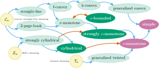
Figure 1: Relations between special drawings (yellow) and classes of simple drawings of $K_{n}$ (seagreen/violet). Arrows indicate that the ?source class? is contained in the ?target class? (concerning weak isomorphism); darkorange arrows are shown in (the appendix of) this work. Conjecture 1 is (now) known to be true for the yellow/seagreen classes; for the darker seagreen ones this is shown below.

Lemma 2.2.

Let $e$ be an edge of a strongly $c$-monotone (with respect to $O$) drawing of $K_{n}$. Then the sub-drawing induced by all vertices in the wedge bounded by the rays from $O$ through the end-vertices of $e$ and containing $e$ is strongly isomorphic to an $x$-monotone drawing.

Lemma 2.3.

In every cylindrical drawing, per circle, there exists at most one edge between neighboring vertices that is crossed by other edges.

Theorem 2.4.

For every cylindrical drawing $\mathcal{D}$ there exists a weakly isomorphic drawing $\mathcal{D}^{\prime}$ that is $c$-monotone. Moreover, for every strongly cylindrical drawing $\mathcal{D}$ there exists a weakly isomorphic drawing $\mathcal{D}^{\prime}$ that is strongly $c$-monotone.

For straight-line drawings of $K_{n}$ it is easy to see that a crossing-free Hamiltonian cycle always exists (for example, pick an arbitrary vertex $v$, visit all other vertices in circular order around $v$, and add $v$ at some position to close the cycle). Further, it was known that every $2$-page-book, $x$-monotone, and strongly cylindrical drawing of $K_{n}$ contains a crossing-free Hamiltonian cycle (see, for example, [4]); however, as we are not aware of a reference containing proofs for these statements, we present such proofs in this work, starting with $x$-monotone and $x$-bounded drawings (which include $2$-page-book drawings as a sub-class). We remark that $2$-page-book drawings of $K_{n}$ with $n\geq 3$ actually contain a Hamiltonian cycle of completely uncrossed edges.

Theorem 2.5.

Every $x$-monotone and every $x$-bounded drawing of the complete graph $K_{n}$ on $n\geq 3$ vertices contains at least one crossing-free Hamiltonian cycle.

Proof 2.6.

First, let $\mathcal{D}$ be an $x$-monotone drawing of $K_{n}$, let the vertices $v_{1},\ldots,v_{n}$ be in that order from left to right in horizontal direction, and see Figure 2 for an example illustration of the construction. Consider the edge $e=\{v_{1},v_{n}\}$ and the Hamiltonian path $\mathcal{P}=v_{1}v_{2}\ldots v_{n}$ (which is crossing-free by the definition of $x$-monotone drawings). If $e$ does not cross $\mathcal{P}$ then $e+\mathcal{P}$ is a crossing-free Hamiltonian cycle. Otherwise, $e$ has $k>0$ crossings with $\mathcal{P}$ and partitions the vertices of $\mathcal{D}\setminus\{v_{1},v_{n}\}$ into a set above $e$ and a set below $e$.

Our goal is to find crossing-free paths $\mathcal{P}_{1}$ and $\mathcal{P}_{2}$ from $v_{1}$ to $v_{n}$, which visit all vertices above and below $e$, respectively. Let $x_{i}$ be the $i$-th crossing between $e$ and $\mathcal{P}$ from left to right (in horizontal direction, which is the same as along $\mathcal{P}$ or $e$). Further, let $v_{a_{i}}$ and $v_{b_{i}}$ be the vertices directly before and after $x_{i}$, respectively. Then the edge $f_{0}$ from $v_{1}$ to $v_{b_{1}}$ and the edge $f_{k}$ from $v_{a_{k}}$ to $v_{n}$ cannot cross $e$ (because $e$ is incident to $f_{0}$ and $f_{k}$). Similarly, for every crossing $x_{i}$ ($1\leq i\leq k-1$) the edge $f_{i}$ from $v_{a_{i}}$ to $v_{b_{i+1}}$ cannot cross $e$ because otherwise, $f_{i}$ and $e$ would have to cross at least twice. In other words, for $1\leq i\leq k$, the edges $f_{i}$ alternate between lying completely above and completely below $e$.

Therefore, the edges $f_{i}$ lying above $e$ combined with all edges of $\mathcal{P}$ that also lie above $e$ (basically, sub-paths of $\mathcal{P}$ from $v_{1}$ or $v_{b_{i-1}}$ to $v_{a_{i}}$ or $v_{n}$) form a crossing-free path $\mathcal{P}_{1}$ from $v_{1}$ to $v_{n}$ (because the edges lie in separate vertical strips and the start-/end-vertices coincide) visiting all vertices above $e$. In the same manner, there is a crossing-free path $\mathcal{P}_{2}$ visiting all vertices below $e$. Then joining $\mathcal{P}_{1}$ and $\mathcal{P}_{2}$ results in a crossing-free Hamiltonian cycle because $e$ separates $\mathcal{P}_{1}$ and $\mathcal{P}_{2}$, which completes the proof for $x$-monotone drawings.

For $x$-bounded drawings, the statement follows from the above proof and Theorem 2.1.

Figure 2: Constructing a crossing-free Hamiltonian cycle in an $x$-monotone drawing of $K_{n}$ from crossing-free paths $\mathcal{P}_{1}$ (darkorange) above and $\mathcal{P}_{2}$ (violet) below the edge $e=\{v_{1},v_{n}\}$ (seagreen).

The result on strongly $c$-monotone drawings follows now almost immediately.

Theorem 2.7.

Every strongly $c$-monotone drawing of the complete graph $K_{n}$ on $n\geq 3$ vertices contains at least one crossing-free Hamiltonian cycle.

Proof 2.8.

Let the vertices $v_{1}$ to $v_{n}$ be in that order counter-clockwise around $O$ and consider the $n$ edges $e_{i}=\{v_{i},v_{i+1}\}$ between neighboring vertices (see Figure 3(a) for visual assistance). If all of them are in the ?short? direction (counter-clockwise from $v_{i}$ to $v_{i+1}$) around $O$, then they form a crossing-free Hamiltonian cycle (by the definition of $c$-monotone drawings) and we are done. Otherwise there is some edge $e_{j}$ (for $1\leq j\leq n$) going the ?long? direction (clockwise from $v_{j}$ to $v_{j+1}$) around $O$. But then the whole drawing is strongly isomorphic to an $x$-monotone drawing by Lemma 2.2 (for which being strongly $c$-monotone is crucial). Therefore we know by Theorem 2.5 that a crossing-free Hamiltonian cycle exists.

(a)

(b)

Figure 3: (a) A crossing-free Hamiltonian cycle in a strongly $c$-monotone drawing of $K_{n}$: Either visiting the vertices in circular order around $O$ is sufficient or the drawing is strongly isomorphic to an $x$-monotone drawing. (b) A strongly $c$-monotone drawing that is neither $x$-monotone nor cylindrical nor generalized convex (the darkorange $K_{5}$ cannot be drawn straight-line).

In Figure 3(b) we give an example of a strongly $c$-monotone drawing that is neither $x$-monotone nor cylindrical (it does not have any uncrossed edge) and also not generalized convex (it contains a non-straight-line drawing of $K_{5}$; confer Arroyo et al. [6]).

We conclude by verifying Conjecture 1 for cylindrical drawings, using the same idea as in a previously known proof for strongly cylindrical drawings. Note that for strongly cylindrical drawings, Conjecture 1 is also true by Theorem 2.4 together with Theorem 2.7.

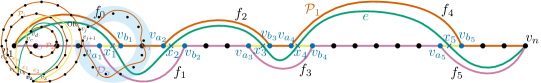
Figure 4: In a cylindrical drawing of $K_{n}$: Connecting the two completely uncrossed paths of rim edges (darkorange) with one of two pairs of lateral edges (seagreen/yellow) to a crossing-free Hamiltonian cycle.

Theorem 2.9.

Every cylindrical drawing of the complete graph $K_{n}$ on $n\geq 3$ vertices contains at least one crossing-free Hamiltonian cycle.

Proof 2.10.

Assume first that there are at least two vertices on each circle and confer Figure 4. Then by Lemma 2.3, every cylindrical drawing contains two completely uncrossed paths $\mathcal{P}_{1}$ and $\mathcal{P}_{2}$ (one per circle) that together contain all vertices. Consider the end-vertices $v_{a}$ and $v_{b}$ of $\mathcal{P}_{1}$, and $v_{c}$ and $v_{d}$ of $\mathcal{P}_{2}$. Then both, the pair of edges $\{v_{a},v_{c}\}$ and $\{v_{b},v_{d}\}$, and the pair $\{v_{a},v_{d}\}$ and $\{v_{b},v_{c}\}$, connect the completely uncrossed paths $\mathcal{P}_{1}$ and $\mathcal{P}_{2}$ to a Hamiltonian cycle. Since there can be at most one crossing in the sub-drawing induced by the four-tuple of vertices $\{v_{a},v_{b},v_{c},v_{d}\}$, at least one of those two Hamiltonian cycles is crossing-free.

Finally, if there is only a single vertex $v$ on one of the circles, then the two edges connecting $v$ to $\mathcal{P}_{2}$, the completely uncrossed path on the other circle, are incident; therefore, they do not cross anyway. And if all vertices lie on the same circle, then the drawing is strongly isomorphic to a $2$-page-book drawing and the result follows from Theorem 2.5.

3 Conclusion

We showed the existence of a crossing-free Hamiltonian cycle in every strongly $c$-monotone drawing and in every cylindrical drawing of $K_{n}$. By Theorem 2.1, we also extended the result to $x$-bounded drawings. Furthermore, this work contains the first published proofs of Conjecture 1 for $2$-page-book, $x$-monotone, and strongly cylindrical drawings.

During our research, in addition, we came up with the following conjecture.

Conjecture 2.

Every simple drawing $\mathcal{D}$ of $K_{n}$ for $n\geq 1$ contains, for each pair of vertices $v_{a}$ and $v_{b}$ in $\mathcal{D}$, a crossing-free Hamiltonian path with end-vertices $v_{a}$ and $v_{b}$.

In Appendix B we show that this conjecture is in fact at least as strong as Conjecture 1.

Theorem 3.1.

A positive answer to Conjecture 2 implies a positive answer to Conjecture 1.

In particular, if Conjecture 2 is true for all simple drawings of $K_{n+1}$ for some $n\geq 3$ then Conjecture 1 is true for all simple drawings of $K_{n}$.

We can confirm Conjecture 2 for all simple drawings on $n\leq 9$ vertices using the rotation system database. In Appendix B, we show it to be true for cylindrical and strongly $c$-monotone drawings as well. A next goal is to extend those results to more classes of simple drawings, especially, generalized twisted drawings on an even number of vertices. Further, the classes of $c$-monotone drawings and crossing maximal drawings are of interest too.

Another intriguing question is to figure out the essential reason why Conjecture 1 should be true in general for simple drawings, while it is not true anymore for star-simple drawings.

Moreover, it would be interesting to know whether Theorem 3.1 can be strengthened to an equivalence of Conjectures 2 and 1. We remark, however, that even if Conjecture 2 is strictly stronger than Conjecture 1, it could potentially be easier to prove.

Acknowledgments.

All results presented in this work are also contained in the Master’s thesis [16] of Joachim Orthaber. We thank Rosna Paul, Daniel Perz, and Alexandra Weinberger for fruitful discussions. We also thank the three anonymous referees for their helpful comments, including the suggestion to use better distinguishable colors in the figures. The colors we now use were recommended in [21].

Appendix A Classes of Simple Drawings and Their Relations

Here we present in detail the results about relations with respect to inclusion between different classes of simple drawings.

$X$-Bounded Drawings.

We start by proving Theorem 2.1. The main ingredient for that is given by the following proposition. Note that in an $x$-bounded or $x$-monotone drawing of $K_{n}$, no two vertices can have the same $x$-coordinate.

Proposition A.1.

Let $e=\{v_{a},v_{b}\}$ be any edge and $v$ any vertex with $x$-coordinate between $v_{a}$ and $v_{b}$ in an $x$-bounded drawing of $K_{n}$. Then $e$ crosses the vertical line through $v$ either above $v$ or below $v$ (at least once) but never on both sides.

Proof A.2.

The edge $e$ divides the vertical strip between $v_{a}$ and $v_{b}$ into an ?upper part? and a ?lower part? (that is, the parts above and below $e$, respectively). Assume, without loss of generality, that $v$ lies in the lower part and that $v_{a}$ is left of $v_{b}$; see Figure 5(a) for visual assistance. Consider now the edges $f_{1}=\{v_{a},v\}$ and $f_{2}=\{v,v_{b}\}$. Since they are both incident to $e$, they cannot cross $e$. Furthermore, the relative interior of $f_{1}$ lies completely in the vertical strip between $v_{a}$ and $v$, the relative interior of $f_{2}$ lies completely in the vertical strip between $v$ and $v_{b}$, and $f_{1}$ and $f_{2}$ meet in $v$ (which lies in the lower part). So $f_{1}$ and $f_{2}$ both lie completely in the lower part (except for the end-vertices $v_{a}$ and $v_{b}$) and the union of $f_{1}$ and $f_{2}$ separates $e$ from the vertical ray that starts in $v$ and goes downwards. Therefore, $e$ can only cross the vertical line through $v$ above $v$ (and $e$ must cross that vertical line at least once to connect $v_{a}$ and $v_{b}$).

(a)

(b)

Figure 5: (a) The edge $e$ can only cross the vertical line through $v$ (violet) on one side (above or below) because $f_{1}$ and $f_{2}$ separate $e$ from the other side (orange area). (b) The edge $e$ crosses the vertical line through $v$ on both sides; the edge $\{v,v_{b}\}$ (dashed darkorange) cannot be inserted anymore within the vertical strip between $v$ and $v_{b}$ without crossing $e$ (which is forbidden).

In Figure 5(b) we hint at another way of proving Proposition A.1 by contradiction, which also indicates that the statement only holds when all $\binom{n}{2}$ edges are present in the drawing.

From here on the proof of Theorem 2.1 is mostly ?just technical?. We start by introducing, for each vertex $v$ of an $x$-bounded drawing, a partial order $<_{v}$ on the set of edges in the drawing, defined by the following four conditions for $e<_{v}f$:

• $e$ and $f$ are incident to $v$, and $e$ leaves $v$ below $f$ on the same side (left or right),

• $e$ crosses the vertical line through $v$ below $v$ and $f$ is incident to $v$,

• $f$ crosses the vertical line through $v$ above $v$ and $e$ is incident to $v$, or

• the vertical line through $v$ is crossed below $v$ by $e$ and above $v$ by $f$.

(a)

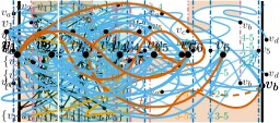
(b)

(c)

Figure 6: (a) A realization of $\mathcal{T}_{5}$ as a (quite wiggly) $x$-bounded drawing. The violet lines mark the bounds for the edges. (b) A Hasse diagram for the partial order $<_{v_{3}}$ of the drawing in (a). (c) A Hasse diagram for the partial order $<_{v_{4}}$ of the drawing in (a).

Any of these four conditions potentially induces an order between two edges, however, by Proposition A.1, the four conditions are non-contradicting. Note that there is no relation between $e$ and $f$ if they both cross the vertical line through $v$ on the same side of $v$. Also, there is no relation between any edge $e$ lying completely to the left of $v$ and any edge $f$ lying completely to the right of $v$. Further, it can easily be verified that antisymmetry and transitivity are fulfilled, and since no edge gets related to itself, the conditions in fact induce a well-defined partial order. In Figure 6 we show two examples of such a partial order of edges at a vertex.

With the following two lemmas we now fully determine all crossings in $x$-monotone drawings just by looking at those partial orders of edges. Also remember that we still have a total order on the vertices from left to right, which we denote by $<$.

Lemma A.3.

Let $\mathcal{D}$ be an $x$-bounded drawing of $K_{n}$. If for two edges $e$ and $f$ and vertices $v<w$ in $\mathcal{D}$ the inequalities $e<_{v}f$ and $e>_{w}f$ hold, then $e$ and $f$ have a crossing in the vertical strip between $v$ and $w$.

Proof A.4.

Consider the area $A$ between the vertical line through $v$ and the vertical line through $w$, excluding a small $\varepsilon$-ball around $v$ and $w$ each (with $\varepsilon$ small enough such that only parts of edges incident to $v$ and $w$, respectively, lie inside the ball); see Figure 7(a) for an example. Further, let the edges $e$ and $f$ be directed from their left to their right end-vertex. Let $e^{\prime}$ be the part of $e$ that starts at the last point where $e$ enters $A$ from the left and that ends at the first point after that where $e$ leaves $A$ to the right (this is well-defined because the end-vertices of $e$ lie to the left and to the right of $A$, respectively). Let $f^{\prime}$ be the part of $f$ that is obtained analogously to $e^{\prime}$ for $e$ ($e^{\prime}$ and $f^{\prime}$ are drawn orange in Figure 7(a)).

Then $e^{\prime}$ enters $A$ strictly below $f^{\prime}$ at the left boundary of $A$ because $e<_{v}f$ (since we excluded an $\varepsilon$-ball around $v$ this also holds if $e$ and $f$ are both incident to $v$). Similarly, $e^{\prime}$ leaves $A$ strictly above $f^{\prime}$ at the right boundary of $A$. So $e^{\prime}$ and $f^{\prime}$ must cross within $A$ and therefore $e$ and $f$ have a crossing in the vertical strip between $v$ and $w$.

For the given order $<$ on the vertices from left to right (indicated by their indices), we call two non-incident edges $e=\{v_{a},v_{b}\}$ and $f=\{v_{c},v_{d}\}$ (without loss of generality $a<c$ and by convention $a<b$ and $c<d$)

• separated, if $a<b<c<d$,

• linked, if $a<c<b<d$, and

• nested, if $a<c<d<b$.

(a)

(b)

Figure 7: (a) Visualization of the proof of Lemma A.3. The orange parts of $e$ and $f$ must cross in area $A$ (shaded seagreen). (b) Visualization of the proof of Lemma A.5 (nested cases on the left and linked cases on the right). The darkorange shaded parts on top mark areas that $e$ cannot enter without crossing $f$ at least twice.

With the next lemma, we relate crossings between edges in an $x$-bounded drawing of $K_{n}$ to their partial orders at (some of) their end-vertices, depending on whether the edges are linked or nested. In other words, we classify in which pattern two edges have to pass below or above each others end-vertices to form a crossing.

Lemma A.5.

Let $\mathcal{D}$ be an $x$-bounded drawing of $K_{n}$ with vertices $v_{1},\ldots,v_{n}$ from left to right. Let $e=\{v_{a},v_{b}\}$ and $f=\{v_{c},v_{d}\}$ (by convention $a<b$ and $c<d$) be two edges in $\mathcal{D}$ with $a\leq c$. Then $e$ and $f$ cross if and only if one of the following two conditions holds:

• $e$ and $f$ are nested and ($e<_{v_{c}}f$ and $e>_{v_{d}}f$) or ($e>_{v_{c}}f$ and $e<_{v_{d}}f$); or

• $e$ and $f$ are linked and ($e<_{v_{c}}f$ and $e>_{v_{b}}f$) or ($e>_{v_{c}}f$ and $e<_{v_{b}}f$).

Proof A.6.

By Lemma A.3, there is a crossing between $e$ and $f$ in the two stated situations (in the vertical strip between $v_{c}$ and $v_{d}$ in the nested case, and in the vertical strip between $v_{c}$ and $v_{b}$ in the linked case; see the two bottom illustrations in Figure 7(b) for an example). So we only have to show that $e$ and $f$ cannot cross in any other case.

If $e$ and $f$ are incident or separated, they obviously cannot cross. Further, if $e$ and $f$ are nested, let without loss of generality $e<_{v_{c}}f$ as well as $e<_{v_{d}}f$ (see Figure 7(b) top left). Then, by crossing $f$, $e$ would enter an area (shaded darkorange) bounded by $f$ and the vertical rays (marked violet) from $v_{c}$ and $v_{d}$ going upwards, which $e$ cannot leave anymore to reach $v_{b}$ (because $e<_{v_{c}}f$, $e<_{v_{d}}f$, and crossing $f$ a second time would violate the property of simple drawings). Similarly, if $e$ and $f$ are linked and, without loss of generality, $e<_{v_{c}}f$ as well as $e<_{v_{b}}f$ (see Figure 7(b) top right), then $e$ cannot cross $f$ either (note that $e$ is $x$-bounded by the vertical line through $v_{b}$ and that a ?forbidden area? might only be bounded by that line and $f$ in this case).

Note that Lemmas A.3 and A.5 hold for arbitrary graphs in the case of $x$-monotone drawings. Indeed, the graph being complete is only needed so that the orders $<_{v}$ are well defined for $x$-bounded drawings.

Further, Lemma A.5 tells us all the crossings in an $x$-bounded drawing and Lemma A.3 helps to narrow down the approximate location of the crossings. With that, we are ready to prove Theorem 2.1.

We note that this theorem is similar to a result shown by Fulek et al. [10]: Every $x$-bounded drawing (not necessarily simple and of an arbitrary graph) can be made $x$-monotone without changing the parity of crossings between any pair of edges or changing the rotation around any vertex.

See 2.1

(a)

(b)

Figure 8: (a) The four steps of redrawing the $x$-bounded drawing from Figure 6(a) strip by strip into a weakly isomorphic $x$-monotone drawing (note that each of the vertices $v_{2}$ to $v_{4}$ appears in two steps). The placement of the pairs ?a-b? (for edges $\{v_{a},v_{b}\}$) from bottom to top corresponds to the orders $<_{i}^{\leftarrow}$ (left boundary of each strip) and $<_{i}^{\rightarrow}$ (right boundary of each strip). The colors of the pairs indicate the three groups, into which the edges are placed in $<_{i}^{\rightarrow}$: Orange for edges leaving the strip below $v_{i+1}$, seagreen for edges incident to $v_{i+1}$, and violet for edges passing above $v_{i+1}$.
(b) The final result after smoothing the edges.

Proof A.7.

We will construct an $x$-monotone drawing $\mathcal{D}^{\prime}$ that has the exact same set of crossing edge pairs as $\mathcal{D}$ (see Figure 8 for an example of the following steps).

First, we place the $n$ vertices in the same order as in $\mathcal{D}$ (without loss of generality, $v_{1},v_{2},\ldots,v_{n}$) from left to right equally spaced on a horizontal line. The goal now is to look at the vertical strips between the vertices from left to right. In each strip we add all the edges simultaneously, by defining orders (from bottom to top) on where the edges enter the strip from the left as well as where they leave the strip to the right. Then we just connect the respective ?entry? and ?exit? points by straight lines.

In detail, we inductively consider the vertical strip between (and including) vertices $v_{i}$ and $v_{i+1}$, for $i=1,\ldots,n-1$. We can assume that all ?entry points from the left? of edges crossing the vertical line through $v_{i}$ below or above $v_{i}$ are given by the ?exit points to the right? in the vertical strip between vertices $v_{i-1}$ and $v_{i}$. Note that, as a basis, for the first strip between vertices $v_{1}$ and $v_{2}$, there are no such edges entering from the left. These entry points induce a linear order of those edges from bottom to top which we denote by $<_{i}^{\leftarrow}$ (the order on the left boundary of the strip between $v_{i}$ and $v_{i+1}$). It remains to add the edges incident to $v_{i}$ to this order.

For that, we insert all the edges incident to $v_{i}$ that leave $v_{i}$ to the right in $\mathcal{D}$ into $<_{i}^{\leftarrow}$ between the edges crossing the vertical line through $v_{i}$ below $v_{i}$ and those crossing the line above $v_{i}$. Moreover, the added edges are ordered according to the order $<_{v_{i}}$ in $\mathcal{D}$ (which is the same as the order given by the counter-clockwise rotation of these edges at $v_{i}$). Note that the resulting order $<_{i}^{\leftarrow}$ agrees with the partial order $<_{v_{i}}$ in $\mathcal{D}$.

Now, we create an order $<_{i}^{\rightarrow}$ (the order on the right boundary of the strip between $v_{i}$ and $v_{i+1}$) of ?exit points to the right?. To this end, we split the edges into three groups, namely, the ones ?passing below? $v_{i+1}$, the ones ?incident? to $v_{i+1}$, and the ones ?passing above? $v_{i+1}$. Note that the edges in each group are in general not consecutive in $<_{i}^{\leftarrow}$. To obtain $<_{i}^{\rightarrow}$, we start with all edges passing below $v_{i+1}$, continue with all edges ending in $v_{i+1}$, and finish with all edges passing above $v_{i+1}$, in each of the groups keeping the relative order between the edges as given by $<_{i}^{\leftarrow}$. Observe that for two edges from different groups, $<_{i}^{\rightarrow}$ agrees with the partial order $<_{v_{i+1}}$ in $\mathcal{D}$.

Finally, we mark the ?exit points? of the edges on the vertical line through $v_{i+1}$, in the order given by $<_{i}^{\rightarrow}$ equally spaced from bottom to top, such that every edge passing below or above $v_{i+1}$ gets its individual exit point, while all edges ending in $v_{i+1}$ share the position of $v_{i+1}$ as their exit point. For each edge, we connect the corresponding ?entry point? on the left boundary of the strip with the ?exit point? on the right boundary of the strip by a straight line segment. Then two of those line segments cross in $\mathcal{D}^{\prime}$ if and only if the order of the corresponding edges (call them $e$ and $f$) changes between $<_{i}^{\leftarrow}$ and $<_{i}^{\rightarrow}$ (without loss of generality, let $e<_{i}^{\leftarrow}f$ and $f<_{i}^{\rightarrow}e$). We next show, by applying Lemma A.3, that each such crossing in $\mathcal{D}^{\prime}$ uniquely corresponds to a crossing of $e$ and $f$ in $\mathcal{D}$.

Since within each of the three groups, we keep the relative order from the left of the strip for the right of the strip, $e$ and $f$ can only cross when they get placed into different groups on the right. Therefore, $f<_{i}^{\rightarrow}e$ implies that $f<_{v_{i+1}}e$ holds.

Regarding the partial order $<_{v_{i}}$, the edges $e$ and $f$ might be incomparable. However, there must be a vertex $w\leq v_{i}$ such that $e$ and $f$ are comparable with respect to $<_{w}$ (this is at least the case for the start-vertex of either $e$ or $f$). So let $k\leq i$ be maximal such that $e$ and $f$ are comparable with respect to $<_{v_{k}}$. In other words, $e$ and $f$ both cross the vertical line through $v_{j}$ on the same side of $v_{j}$ for all $k<j\leq i$ (since they are incomparable in that range). Therefore, $e<_{i}^{\leftarrow}f$ implies $e<_{k}^{\leftarrow}f$ (since $<_{j-1}^{\rightarrow}$ agrees with $<_{j}^{\leftarrow}$ for all $j$ and $<_{j-1}^{\leftarrow}$ agrees with $<_{j-1}^{\rightarrow}$ for edges that get placed into the same group). Consequently, we get $e<_{v_{k}}f$ (since $e$ and $f$ are comparable with respect to $<_{v_{k}}$, which agrees with $<_{k}^{\leftarrow}$). Hence, by Lemma A.3, $e$ and $f$ cross in the vertical strip between vertices $v_{k}$ and $v_{i+1}$ in $\mathcal{D}$.

Moreover, $e$ and $f$ are comparable with respect to $<_{v_{i+1}}$. So any potential further crossing between $e$ and $f$ in $\mathcal{D}^{\prime}$ would correspond to a crossing between $e$ and $f$ in $\mathcal{D}$ that lies to the right of the vertical line through $v_{i+1}$. This cannot exist since $\mathcal{D}$ is simple.

It remains to argue that every crossing in $\mathcal{D}$ also exists in $\mathcal{D}^{\prime}$. By Lemma A.5, we know that every crossing in $\mathcal{D}$ is in one-to-one correspondence with a change of the order of the involved edges $e$ and $f$ between two partial orders $<_{v_{i}}$ and $<_{v_{j}}$ with $i<j$ (that is, at two of the end-vertices of $e$ and $f$). This change implies that also the orders $<_{i}^{\leftarrow}$ and $<_{j}^{\rightarrow}$ change accordingly (since crossing edges are always non-incident), which produces a crossing in the construction of $\mathcal{D}^{\prime}$.

Finally, to get an $x$-monotone drawing $\mathcal{D}^{\prime}$, we can smooth the transitions of edges between the strips to avoid sharp bends, and, if necessary, slightly move transition points between strips in vertical direction to avoid three or more edges passing through a common point in their relative interiors.

Note that in this construction, edges cross at the latest possible moment (that is, in the rightmost strip of the area given by Lemma A.3). Also note that we implicitly use Proposition A.1 all the time because the orders $<_{v_{i}}$ would not be well defined otherwise. In fact, Theorem 2.1 does not hold for drawings of non-complete graphs. For example, Figure 9(a) depicts an $x$-bounded drawing $\mathcal{D}_{b}$ for which, as we show in the following, no weakly isomorphic $x$-monotone drawing $\mathcal{D}_{m}$ exists.

(a)

(b)

(c)

Figure 9: (a) An $x$-bounded drawing $\mathcal{D}_{b}$ of a non-complete graph that is not weakly isomorphic to any $x$-monotone drawing; the darkorange edge is $x$-bounded but not $x$-monotone. (b) An illustration showing that there cannot be any $x$-monotone drawing $\mathcal{D}_{m}$ on the given vertex order being weakly isomorphic to $\mathcal{D}_{b}$. (c) An $x$-monotone drawing $\mathcal{D}_{m}^{\prime}$ which is weakly isomorphic to a sub-drawing of $\mathcal{D}_{b}$ but has a different (partial) rotation system.

Potentially, we would have to try all $360$ possible orders (permutations modulo reflection) of the vertices along the $x$-axis. However, using the fact that in $x$-monotone (actually even $x$-bounded) drawings two separated edges cannot cross and, especially, that the edges $\{v_{1},v_{2}\}$ and $\{v_{n-1},v_{n}\}$ must be completely uncrossed, reduces this to $40$ potential orders for the drawing $\mathcal{D}_{m}$. Further, if an edge $e$ crosses a triangle $\Delta$ an odd number of times (for example, the edge $\{v_{3},v_{6}\}$ crosses the triangle $\{v_{2},v_{4},v_{5}\}$ once in $\mathcal{D}_{b}$), then one of the end-vertices of $e$ must lie inside $\Delta$ and the other one outside. In particular, for $x$-monotone (and $x$-bounded) drawings, $\Delta$ can never be nested within the end-vertices of $e$ because then both end-vertices definitely lie outside of $\Delta$ (as it would happen, for example, with the order $(v_{3},v_{1},v_{2},v_{4},v_{5},v_{6})$ for $\mathcal{D}_{m}$). This eliminates $19$ more orders.

To rule out the remaining $21$ cases, recall that Lemma A.5 also holds for non-complete graphs in the case of $x$-monotone drawings. So, for example (see Figure 9(b) for visual assistance), for the order $(v_{1},v_{2},v_{3},v_{4},v_{5},v_{6})$ we can first add the edge $\{v_{1},v_{6}\}$; let, without loss of generality, $v_{2}$ lie below $\{v_{1},v_{6}\}$, then $v_{3}$ has to lie above $\{v_{1},v_{6}\}$ because $\{v_{2},v_{3}\}$ crosses $\{v_{1},v_{6}\}$, $v_{4}$ also has to lie above $\{v_{1},v_{6}\}$ because $\{v_{3},v_{4}\}$ does not cross $\{v_{1},v_{6}\}$, and $v_{5}$ has to lie below $\{v_{1},v_{6}\}$ again because $\{v_{4},v_{5}\}$ crosses $\{v_{1},v_{6}\}$. Further, the edge $\{v_{2},v_{6}\}$ lies below $v_{4}$ and does not cross $\{v_{4},v_{5}\}$, so it has to lie below $v_{5}$ as well. Finally, the edge $\{v_{1},v_{5}\}$ has to lie below $v_{2}$ to cross $\{v_{2},v_{6}\}$, but then it cannot cross $\{v_{2},v_{3}\}$ and $\{v_{2},v_{4}\}$ anymore. This finishes the proof that there is no $x$-monotone drawing $\mathcal{D}_{m}$ on this order of vertices being weakly isomorphic to $\mathcal{D}_{b}$. The remaining $20$ cases can be argued similarly.

Note, however, that removing the edges $\{v_{3},v_{6}\}$ and $\{v_{4},v_{6}\}$ from $\mathcal{D}_{b}$ creates a sub-drawing $\mathcal{D}_{b}^{\prime}$ for which a weakly isomorphic $x$-monotone drawing $\mathcal{D}_{m}^{\prime}$ exists; it is reached by changing the position of the edges $\{v_{2},v_{4}\}$ and $\{v_{3},v_{5}\}$ in the rotation of their end-vertices though (see Figure 9(c)), which also shows that for drawings of non-complete graphs two different (partial) rotation systems can produce the same set of crossing edge pairs.

Also note that in $\mathcal{D}_{b}$, only the three edges $\{v_{1},v_{3}\}$, $\{v_{1},v_{4}\}$, and $\{v_{5},v_{6}\}$ are missing, which cannot be added in an $x$-bounded way anymore (recall Figure 5(b)). We can easily add all three of them simultaneously to get a (general) simple drawing of the complete graph $K_{6}$ though.

Cylindrical Drawings.

Before we continue with the remaining missing proofs from the main part of this paper, we give some terminology and basic properties of cylindrical drawings: We call the area outside the outer circle, between the two circles, and inside the inner circle in a cylindrical drawing outer, lateral, and inner face, respectively. Additionally, we call edges connecting two vertices from different circles lateral edges and edges connecting two vertices on the inner or outer circle (inner or outer, respectively) circle edges. In particular, we call circle edges connecting two neighboring vertices on their circle rim edges (see Figure 10(a) for an example of those terms).

(a)

(b)

Figure 10: (a) Hill’s drawing on $11$ vertices in the plane. The two concentric circles are drawn violet. Rim edges are seagreen, all other circle edges are orange, and lateral edges are lightblue. (b) Illustrations of the three examples for the continuous winding number of an edge in a cylindrical drawing.

Obviously all lateral edges have to lie in the lateral face. In contrast to that, however, inner (outer, respectively) circle edges can lie either in the inner (outer, respectively) face or in the lateral face. Also note that the sub-drawing induced by all vertices on the same circle is a $2$-page-book drawing.

For the following, we direct all lateral edges from the outer to the inner circle. We direct a circle edge $e=\{v_{a},v_{b}\}$ from $v_{a}$ to $v_{b}$ if, in counter-clockwise direction along its circle, there are fewer vertices between $v_{a}$ and $v_{b}$ than between $v_{b}$ and $v_{a}$ (we direct $e$ arbitrarily if the two numbers are the same). We now define, similar to the winding number of closed curves in complex analysis, the continuous winding number $\omega_{e}$ of an edge $e$ as the overall portion of times (as a real number) $e$ completely travels (in the above described direction) around the common center of the two circles (denoted by $O$ for ?origin?) in counter-clockwise direction.

See Figure 10(b) for three examples: First, if a lateral edge $e$ (orange) travels around $O$ one and a half times (that is, the end-vertex is opposite from the start-vertex with regard to $O$) in clockwise direction, then $\omega_{e}=-1.5$. Second, if a lateral edge $f$ (lightblue) first makes one full round in counter-clockwise direction encircling $O$, then turns around and makes another full round back in clockwise direction, then $\omega_{f}=0$. Finally, note that for a circle edge $g$ (seagreen), the sign of $\omega_{g}$ depends on the distribution of vertices on the respective circle; in the given example we have $\omega_{g}>0$. Also note that we can assume, without loss of generality, that no circle edge actually passes through $O$, so that we have the continuous winding number well-defined for all edges.

We can give a bound on $\omega_{e}$, simultaneously for every edge $e$ in a cylindrical drawing.

Lemma A.8.

For every cylindrical drawing $\mathcal{D}$ there exists a strongly isomorphic cylindrical drawing $\mathcal{D}^{\prime}$ such that $\lvert\omega_{e}\rvert<1$ for every edge $e$ in $\mathcal{D}^{\prime}$.

Proof A.9.

Observe that $\lvert\omega_{e}\rvert<1$ holds anyway for every circle edge $e$ because otherwise $e$ would have to cross itself. Let further $e_{0}$ and $e_{1}$ be two lateral edges for which $\omega_{e_{0}}=\min_{e\in E}(\omega_{e})$ and $\omega_{e_{1}}=\max_{e\in E}(\omega_{e})$ holds, where $E$ is the set of all lateral edges in $\mathcal{D}$. Observe that $\omega_{e_{1}}-\omega_{e_{0}}<2$ because otherwise $e_{0}$ and $e_{1}$ would have to cross each other at least twice.

So we can rotate, for example, the outer circle appropriately (and at the same time rotate the outer face in the same manner, while we deform the lateral face in a homeomorphic way, and keep the inner face as it is) to obtain a cylindrical drawing $\mathcal{D}^{\prime}$ with $\lvert\omega_{e}\rvert<1$ for every edge $e$ in it.

$C$-Monotone Drawings.

In the following we prove Lemmas 2.2 and 2.3, which we reformulate here as Corollaries A.18 and A.14, respectively, using terminology that we did not yet have in the main part. Further, we state and prove Propositions A.10 and A.22, which we had merged to Theorem 2.4 in the main part due to space reasons.

We note at this point that Ruiz-Vargas [19] defines ?cylindrical drawings? as arbitrary drawings on the surface of an infinite open cylinder and that his ?monotone cylindrical drawings? are equivalent to our $c$-monotone drawings. The name ?$c$-monotone? is an abbreviation for ?circularly monotone? and meant as a generalization of $x$-monotone drawings.

Proposition A.10.

For every cylindrical drawing $\mathcal{D}$ there exists a weakly isomorphic drawing $\mathcal{D}^{\prime}$ that is $c$-monotone.

Proof A.11.

We aim to construct $\mathcal{D}^{\prime}$ to be $c$-monotone with respect to the common center $O$ of the two circles that host all vertices of $\mathcal{D}$. By Lemma A.8, we can assume, without loss of generality, that $\lvert\omega_{e}\rvert<1$ holds for every edge $e$ in $\mathcal{D}$. This is a fundamental requirement for the edges to potentially be $c$-monotone with respect to $O$.

Further, all circle edges that lie in the outer or inner face we can draw $c$-monotone with respect to $O$; for example, by drawing them as $c$-monotone arcs arbitrarily close to the respective circle. Note that this does not change which edge pairs cross, as the sub-drawing formed by all edges lying in the outer (inner, respectively) face is weakly isomorphic to a convex straight-line drawing and independent from the rest of $\mathcal{D}$. Similarly, we can draw all circle edges in the lateral face $c$-monotone, noting in addition that a circle edge $\{v_{a},v_{b}\}$ in the lateral face that goes in counter-clockwise order from $v_{a}$ to $v_{b}$ crosses exactly all lateral edges that have one end-vertex between $v_{a}$ and $v_{b}$ in counter-clockwise order on that circle; see Figure 11(a) for an illustration.

Finally, the crossings between lateral edges are uniquely determined by the positions of their end-vertices and their continuous winding numbers: Two lateral edges $e$ and $f$ do not cross if and only if $0\leq\delta+\omega_{f}-\omega_{e}\leq 1$, where $\delta$ is the fraction of the outer circle from the end-vertex of $e$ to the end-vertex of $f$ in counter-clockwise direction. Therefore, we can also replace all lateral edges by $c$-monotone edges (with respect to $O$) while keeping their $\omega_{e}$ values and crossing properties.

(a)

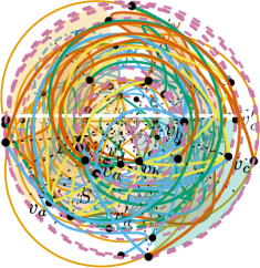
(b)

Figure 11: (a) The lateral edge $f$ (solid lightblue) must cross the circle edge $e$ (darkorange) to leave the orange shaded area bounded by $e$ and the inner circle. Conversely, the lateral edge $f^{\prime}$ (dash dotted lightblue) cannot cross $e$ because it would not be able to leave the orange area again. Similarly, the circle edge $g$ (seagreen) cannot leave the orange area. (b) The wedges of a lateral edge (lightblue/seagreen) and of a circle edge (dark-/orange) in a $c$-monotone cylindrical drawing.

From now on we can assume all cylindrical drawings to be $c$-monotone with respect to the center $O$ of the two circles. For convenience, given a simple drawing $\mathcal{D}$ that is $c$-monotone with respect to some point $O$ of the plane and given an edge $e$ in $\mathcal{D}$, we define the wedge of $e$ to be the wedge with apex $O$, bounded by the rays from $O$ through the end-vertices of $e$, and containing $e$ (including its end-vertices); see Figure 11(b) for two examples (in a cylindrical drawing to emphasize that, by Proposition A.10, we can also use the terminology there).

Lemma A.12.

Let $e=\{v_{a},v_{b}\}$ be a circle edge on circle $C$ of a ($c$-monotone) cylindrical drawing. Let further $g=\{v_{c},v_{d}\}$ be a circle edge on the same circle $C$ and with $v_{c}$ and $v_{d}$ in the wedge of $e$. If $g$ lies on the same side of $C$ as $e$, then $g$ is contained in the wedge of $e$. That is, the sign of $\omega_{g}$ is uniquely determined in that case.

Proof A.13.

In the described setting, $g$ must lie within the area bounded by $e$ and $C$ that does not contain $O$; see the seagreen edge in the shaded orange area in Figure 11(a) for an example (in a slightly more general setting). Indeed, $g$ can neither cross $C$ nor cross $e$ more than once. Hence, $g$ must take the ?same direction? around $O$ as $e$.

From this we can easily derive Lemma 2.3 (restated here using the additional terminology). Remember that the sign of $\omega_{e}$, for a circle edge $e$, describes in which direction $e$ travels around $O$: $\omega_{e}>0$ means the ?shorter? and $\omega_{e}<0$ the ?longer? direction (measured by the number of vertices on the way).

Corollary A.14.

In every cylindrical drawing there exists at most one rim edge per circle that is crossed by other edges.

Proof A.15.

Consider, without loss of generality, the outer circle. First, if a rim edge $e$ is drawn in the outer face, then it is uncrossed anyway. Further, if $e$ is drawn in the lateral face with $\omega_{e}>0$, then it is uncrossed as well. Finally, if $e$ is drawn in the lateral face with $\omega_{e}<0$, then $e$ can have crossings. However, by Lemma A.12, in that case we have $\omega_{f}>0$ for all other rim edges $f$ on the outer circle being drawn in the lateral face; so by the first two cases, all other rim edges are uncrossed.

The following lemma gives an alternative characterization of strongly $c$-monotone drawings in the case of complete graphs. For non-complete graphs the second condition is stronger.

Lemma A.16.

Let $\mathcal{D}$ be a $c$-monotone drawing of $K_{n}$. Then the following are equivalent:

1. $\mathcal{D}$ is strongly $c$-monotone.

2. For every pair of edges $e$ and $f$ in $\mathcal{D}$ there exists a ray starting at $O$ that crosses neither $e$ nor $f$.

Proof A.17.

Assume first that $\mathcal{D}$ is not strongly $c$-monotone. Then there exists a star $\mathcal{S}$ of a vertex $v_{a}$ such that every ray starting at $O$ crosses at least one edge of $\mathcal{S}$. Let $e=\{v_{a},v_{b}\}$ be the edge of $\mathcal{S}$ that goes farthest around $O$ in counter-clockwise order and $f=\{v_{a},v_{c}\}$ be the edge of $\mathcal{S}$ that goes farthest around $O$ in clockwise order. Then the union of the wedge of $e$ and the wedge of $f$ is the whole plane (otherwise there would be a ray not crossing any edge of $\mathcal{S}$). Therefore, $e$ and $f$ form a pair of edges contradicting the second condition of the lemma (see Figure 12(a) for an example).

On the other hand, assume that two edges $e=\{v_{a},v_{b}\}$ and $f=\{v_{c},v_{d}\}$ violate the second condition. If $e$ and $f$ are incident, then obviously there exists a star violating the first condition. Otherwise the wedge of $e$ and the wedge of $f$ intersect in two wedges with apex $O$; without loss of generality, between $v_{a}$ and $v_{c}$, and between $v_{b}$ and $v_{d}$ (shaded darkorange in Figure 12(b)). Consider the edge $g=\{v_{a},v_{d}\}$: Either $g$ is contained in the wedge of $e$, then the star of vertex $v_{d}$ violates the first condition of the lemma, or $g$ is contained in the wedge of $f$, then the star of vertex $v_{a}$ violates the first condition of the lemma.

(a)

(b)

(c)

Figure 12: Illustration of Lemma A.16: (a) A star violating condition $1)$ contains two edges (lightblue) violating condition $2)$, and (b) two non-incident edges (lightblue) violating condition $2)$ enforce a star (of one of the two darkorange vertices) violating condition $1)$; (c) therefore the wedge of any edge $e$ (shaded seagreen) induces an $x$-monotone drawing (Corollary A.18).

Lemma 2.2 (restated here with the additional terminology) is now a direct consequence.

Corollary A.18.

For each edge $e=\{v_{a},v_{b}\}$ in a strongly $c$-monotone drawing of $K_{n}$, the sub-drawing $\mathcal{D}_{e}$ induced by all vertices in the wedge of $e$ is strongly isomorphic to an $x$-monotone drawing.

Proof A.19.

By condition $2)$ of Lemma A.16, $\mathcal{D}_{e}$ must lie completely inside the wedge of $e$ (shaded seagreen in Figure 12(c)). Therefore, we can homeomorphicly deform the plane (mapping vertices onto a horizontal line and $O$ to infinity) to get an $x$-monotone drawing $\mathcal{D}_{e}^{\prime}$ that is strongly isomorphic to $\mathcal{D}_{e}$.

We conclude with the inclusion of strongly cylindrical drawings in strongly $c$-monotone drawings. Note that the sub-drawing of all lateral edges (which corresponds to a non-complete graph) of a cylindrical drawing (assuming it to be $c$-monotone by Proposition A.10) is always strongly $c$-monotone (since incident edges cannot cross). However, two non-incident lateral edges $e=\{v_{a},v_{b}\}$ and $f=\{v_{c},v_{d}\}$ might violate condition $2)$ of Lemma A.16; in that case the signs of $\omega_{e}$ and $\omega_{f}$ must be the same though (otherwise $e$ and $f$ would cross each other twice). We call such a pair of lateral edges with negative signs a clockwise double-spiral (see Figure 13(a) for an example) and with positive signs a counter-clockwise double-spiral.

Proposition A.20.

For every cylindrical drawing $\mathcal{D}$ there exists a weakly isomorphic cylindrical drawing $\mathcal{D}^{\prime}$ without double-spirals.

Proof A.21.

We will move around vertices on the inner circle by homeomorphicly deforming the plane close to the circle (so especially without changing the circular order of the vertices on it) to remove one double-spiral at a time. Note that, by Proposition A.10, we can always assume that the resulting drawing after moving some vertices is still $c$-monotone.

Let $e=\{v_{a},v_{b}\}$ and $f=\{v_{c},v_{d}\}$ form a clockwise double-spiral with $v_{a}$ and $v_{c}$ on the outer circle (see Figure 13(b) for an illustration of the following). Let further $v_{a}^{\prime}$ be the neighboring vertex of $v_{a}$ on the outer circle in counter-clockwise order. Then move vertex $v_{d}$ (and each vertex in its path, to keep the circular order of vertices and therefore weak isomorphism) on the inner circle in counter-clockwise direction into the wedge $S$ with apex $O$, between $v_{a}$ and $v_{a}^{\prime}$ (between the dotted black lines). This removes the double spiral formed by $e$ and $f$.

It remains to show that no new double-spirals are created in the process. Since we only move vertices on the inner circle in counter-clockwise order, we cannot create any new clockwise double-spiral in that process. Let $v_{d}^{\prime}$ be one of the vertices that is moved and let $f^{\prime}=\{v_{c}^{\prime},v_{d}^{\prime}\}$ (darkorange) be an edge with $\omega_{f^{\prime}}>0$ (potentially after $v_{d}^{\prime}$ is moved). Then there exist wedges $S_{1}$ between $v_{d}^{\prime}$ and $v_{a}^{\prime}$ and $S_{2}$ between $v_{c}$ and $v_{c}^{\prime}$ (shaded seagreen) which are disjoint (even if $v_{a}^{\prime}=v_{c}$ or $v_{b}\in S$) and both do not contain any point of $f^{\prime}$. Moreover, any edge $e^{\prime}$ with $\omega_{e^{\prime}}>0$ passing through $S_{1}$ must start at latest (in counter-clockwise direction) at vertex $v_{a}$ on the outer circle and therefore end before vertex $v_{b}$ on the inner circle; so $e^{\prime}$ cannot pass through $S_{2}$ at the same time. Hence, $f^{\prime}$ cannot be part of any counter-clockwise double-spiral.

To remove counter-clockwise double-spirals we proceed similarly (moving vertices on the inner circle in clockwise direction). In each of those steps, we reduce the total number of double-spirals by at least one. So after finitely many steps we reach a weakly isomorphic cylindrical drawing $\mathcal{D}^{\prime}$ without double-spirals.

(a)

(b)

(c)

Figure 13: (a) A clockwise double-spiral (lightblue). The circle edge $\{v_{b},v_{d}\}$ (darkorange) cannot be inserted in a strongly $c$-monotone way (either the solid or the dash dotted edge pairs form an obstruction). (b) Moving vertex $v_{d}$ (and potentially other vertices $v_{d}^{\prime}$) to resolve the clockwise double-spiral; this cannot create a new counter-clockwise double-spiral. (c) A clockwise (lightblue) and a counter-clockwise (seagreen) double-spiral in one drawing. The remaining lateral edges (yellow) can be added while keeping simplicity of the drawing.

Note that the ?weakly? in Proposition A.20 is only due to keeping the drawing $c$-monotone (which we do for convenience because it makes the definition of double-spirals easier). Also, it is possible that a cylindrical drawing (even of a complete graph) contains a clockwise and a counter-clockwise double-spiral at the same time (see Figure 13(c)).

Theorem A.22.

For every strongly cylindrical drawing $\mathcal{D}$ there exists a weakly isomorphic drawing $\mathcal{D}^{\prime}$ that is strongly $c$-monotone.

Proof A.23.

As noted before, after making the drawing $c$-monotone (Proposition A.10), the sub-drawing of lateral edges is strongly $c$-monotone anyway, and, by Proposition A.20, we can assume that there are no double-spirals. The remaining task is to fit all the circle edges, without violating strong $c$-monotonicity or simplicity of the drawing.

First note that each circle edge $e=\{v_{a},v_{b}\}$ (lightblue in Figure 14(a)) has potentially two directions to go around $O$ and that a double-spiral (of lateral edges incident to $v_{a}$ and $v_{b}$, respectively) would be the only structure which prohibits both directions (considering only the stars of $v_{a}$ and $v_{b}$). Since there are no double-spirals, each circle edge $e$ has at least one direction still available. However, if $e$ is forced into one of the two directions by an incident lateral edge $f$ (darkorange), then, by Lemma A.12, $e$ also forces other circle edges $e^{\prime}$ (yellow) to take ?the same direction?. So we have to check that $e^{\prime}$ is not forced into the other direction by an incident lateral edge $f^{\prime}$. Indeed, $f^{\prime}$ would either have two points with $f$ in common (solid seagreen) or form a double-spiral with $f$ (dash dotted seagreen); a contradiction in both cases.

Hence, none of the circle edges that are forced into one direction (by some incident lateral edge or by another circle edge) cross each other twice. Finally, if there are any circle edges left with both choices, we can ?arbitrarily? (respecting Lemma A.12) choose their directions. This produces a strongly $c$-monotone drawing $\mathcal{D}^{\prime}$ which is weakly isomorphic to $\mathcal{D}$.

(a)

(b)

Figure 14: (a) An illustration of the proof of Theorem A.22: Two circle edges $e$ and $e^{\prime}$ cannot be forced into ?different? directions (crossing each other twice) by incident lateral edges ($f$ and $f^{\prime}$). (b) A sub-drawing of a (general) cylindrical drawing that cannot be made strongly $c$-monotone by moving vertices along the circles.

Note that it is essential that the initial drawing $\mathcal{D}$ is ?strongly? cylindrical, because when a circle edge is drawn in the lateral face, then its direction around $O$ is fixed from the start. In particular, Figure 14(b) shows a structure with two circle edges (darkorange) in the lateral face, where the stars of two of the four involved vertices (especially the lightblue and darkorange edges) always violate strong $c$-monotonicity, no matter how the vertices are moved along the circles (without changing their circular order on any circle).

(Generalized) Twisted Drawings.

For completeness, we conclude this section with a definition of twisted drawings: We call a simple drawing of $K_{n}$ twisted if there exists an order on its vertices such that two edges cross if and only if they are nested (see [17]). In the following, we will always use this special order to label the vertices of the twisted drawing $\mathcal{T}_{n}$ from $v_{1}$ to $v_{n}$. In Figure 15(a) we show an example of a ?usual? way of how to realize such a drawing (see also [13, 14]). Furthermore, twisted drawings can be drawn $c$-monotone such that there exists a ray starting at $O$ that crosses all edges (Figure 15(b) shows an example). This is then the defining property of generalized twisted drawings (see [5] for details).

(a)

(b)

Figure 15: The twisted drawing $\mathcal{T}_{6}$ drawn (a) in a ?usual? way and (b) as a $c$-monotone drawing.

Appendix B All Pairs Hamiltonian Paths

We start by proving Theorem 3.1.

See 3.1

Proof B.1.

Let $\mathcal{D}$ be an arbitrary simple drawing of $K_{n}$ for some $n\geq 3$ and assume Conjecture 2 to be true for all simple drawings of $K_{n+1}$. Consider a vertex $v\in\mathcal{D}$ and assume, for simplicity and without loss of generality, that $v$ lies on the boundary of the unbounded cell, that all other vertices lie on a horizontal line above $v$, and that the star of $v$ consists only of straight-line edges going upwards (see Figure 16 on the left; this can be achieved by homeomorphic deformations of the plane/sphere).

Now, we produce a drawing $\mathcal{D}^{\prime}$ of $K_{n+1}$ by splitting $v$ into two vertices $v_{a}$ and $v_{b}$ (see Figure 16 on the right). We duplicate all the edges incident to $v$, so that they are still straight-line and going upwards from $v_{a}$ and $v_{b}$, respectively. Moreover, we place $v_{a}$ and $v_{b}$ close enough to the original position of $v$, one slightly to the left the other slightly to the right, so that any edge $\{v_{a},v_{c}\}$ ($\{v_{b},v_{c}\}$, respectively) in $\mathcal{D}^{\prime}$ has the same crossings as $\{v,v_{c}\}$ had in $\mathcal{D}$. Finally, we connect $v_{a}$ and $v_{b}$ by a completely uncrossed horizontal edge $e$. Then $\mathcal{D}^{\prime}$ is a simple drawing of $K_{n+1}$.

So, by the assumption, $\mathcal{D}^{\prime}$ contains a crossing-free Hamiltonian path $\mathcal{P}$ with end-vertices $v_{a}$ and $v_{b}$. Because $n+1\geq 4$, $\mathcal{P}$ uses neither $e$ nor both edges $\{v_{a},v_{c}\}$ and $\{v_{b},v_{c}\}$ for any vertex $v_{c}$ in $\mathcal{D}^{\prime}$. Therefore, merging $v_{a}$ and $v_{b}$ again to one vertex $v$ transforms $\mathcal{P}$ into a crossing-free Hamiltonian cycle in $\mathcal{D}$. Since $\mathcal{D}$ was arbitrary and the argument works for all $n\geq 3$, this finishes the proof.

Figure 16: A bijection between all simple drawings of $K_{n}$ (left) and certain simple drawings of $K_{n+1}$ (right).

We remark that the above proof does not imply an analogue statement of Theorem 3.1 restricted to only a sub-class of all simple drawings. In other words, showing Conjecture 2 to be true for some class $X$ does not directly imply that Conjecture 1 also holds for all drawings of $X$. For such an implication, we first would have to show that the drawing $\mathcal{D}^{\prime}$ in the proof of Theorem 3.1 can be created in such a way that it lies in the same class as $\mathcal{D}$ (which can potentially be done for all classes considered in this paper though).

Since searching for crossing-free Hamiltonian paths between all pairs of vertices is a new question, we first convince ourselves that Conjecture 2 is true for straight-line drawings.

Proposition B.2.

Every straight-line drawing $\mathcal{D}$ of $K_{n}$ contains, for each pair of vertices $v_{a}$ and $v_{b}$ in $\mathcal{D}$, a crossing-free Hamiltonian path with end-vertices $v_{a}$ and $v_{b}$.

Proof B.3.

If $v_{a}$ or $v_{b}$ (without loss of generality, $v_{a}$) lies inside the convex hull of the vertex set, then, starting from $v_{a}$, we visit all vertices in circular order around $v_{a}$, starting at the vertex after $v_{b}$, until we reach $v_{b}$ (see Figure 17(a)). If both $v_{a}$ and $v_{b}$ lie on the convex hull, then we first visit the vertices on the convex hull in clockwise direction from $v_{a}$ to $v_{b}^{\prime}$ (the vertex before $v_{b}$, where $v_{b}^{\prime}=v_{a}$ is possible), followed by all not yet visited vertices in circular counter-clockwise order around $v_{b}^{\prime}$, again such that $v_{b}$ is last (see Figure 17(b)). In both cases this clearly results in a crossing-free Hamiltonian path with end-vertices $v_{a}$ and $v_{b}$.

(a)

(b)

(c)

Figure 17: Finding a crossing-free Hamiltonian path (lightblue) between two given vertices (darkorange) in a straight-line drawing: (a) If at least one of those two vertices lies inside the convex hull and (b) if both vertices lie on the convex hull. (c) Finding a crossing-free Hamiltonian path containing a specific edge $e$.

As we show next, in straight-line drawings of $K_{n}$ it is also possible to choose an arbitrary edge to be part of a crossing-free Hamiltonian path. This is in general not possible in simple drawings. For example, choose the edge $\{v_{1},v_{n}\}$ in the twisted drawing; since it crosses all non-incident edges, it cannot be part of any crossing-free path with more than three edges.

Proposition B.4.

Every straight-line drawing $\mathcal{D}$ of $K_{n}$ contains for each edge $e$ in $\mathcal{D}$ a crossing-free Hamiltonian path containing $e$.

Proof B.5.

Let the edge $e=\{v_{a},v_{b}\}$, without loss of generality, be vertical (see Figure 17(c)). Consider the sub-drawing $\mathcal{D}_{1}$ induced by the vertices on the left side of $e$ including $v_{a}$ and the sub-drawing $\mathcal{D}_{2}$ induced by the vertices on the right side of $e$ including $v_{b}$. Then there exists a crossing-free Hamiltonian cycle $\mathcal{C}_{1}$ in $\mathcal{D}_{1}$ and a crossing-free Hamiltonian cycle $\mathcal{C}_{2}$ in $\mathcal{D}_{2}$. Removing one edge incident to $v_{a}$ in $\mathcal{C}_{1}$ and one edge incident to $v_{b}$ in $\mathcal{C}_{2}$ and adding the edge $e$ creates a crossing-free Hamiltonian path in $\mathcal{D}$, containing $e$.

We finish by proving Conjecture 2 for cylindrical and strongly $c$-monotone drawings.

Lemma B.6.

Let $e=\{v_{a},v_{b}\}$ be an edge of an $x$-monotone drawing $\mathcal{D}$ and let $\mathcal{D}^{\prime}$ be any sub-drawing of $\mathcal{D}$ containing only vertices between $v_{a}$ and $v_{b}$ in $x$-direction that lie above (below, respectively) $e$ (and potentially including $v_{a}$ and/or $v_{b}$). Then $\mathcal{D}^{\prime}\setminus\{e\}$ lies completely above (below, respectively) $e$.

Proof B.7.

All edges $f=\{v_{c},v_{d}\}$ of $\mathcal{D}^{\prime}\setminus\{e\}$ are either incident to $e$ or nested within the end-vertices of $e$. So, by Lemma A.5, those edges $f$ do not cross $e$. Therefore, the whole sub-drawing $\mathcal{D}^{\prime}$ lies completely on the respective side of $e$, potentially containing $e$ if both $v_{a}$ and $v_{b}$ are part of $\mathcal{D}^{\prime}$.

Proposition B.8.

Every $x$-monotone drawing $\mathcal{D}$ of $K_{n}$ contains, for each pair of vertices $v_{a}$ and $v_{b}$ in $\mathcal{D}$, a crossing-free Hamiltonian path with end-vertices $v_{a}$ and $v_{b}$.

Proof B.9.

We prove this by induction on $n$. For $n\leq 3$ the statement is obviously true. Now let the vertices $v_{1},\ldots,v_{n}$ be in that order from left to right in horizontal direction.

Let first $v_{a}$ and $v_{b}$ lie on different sides of the edge $e=\{v_{1},v_{n}\}$ (without loss of generality, $v_{a}$ above and $v_{b}$ below; see Figure 18(a)). Then the sub-drawing induced by all vertices above (below, respectively) $e$ including $v_{1}$ ($v_{n}$, respectively) is a proper sub-drawing of $\mathcal{D}$ and clearly $x$-monotone. So by the induction hypothesis, there exists a crossing-free path $\mathcal{P}_{1}$ with end-vertices $v_{a}$ and $v_{1}$, visiting all vertices above $e$, and another crossing-free path $\mathcal{P}_{2}$ with end-vertices $v_{b}$ and $v_{n}$, visiting all vertices below $e$. Combining $\mathcal{P}_{1}$ and $\mathcal{P}_{2}$ via $e$ creates a Hamiltonian path with end-vertices $v_{a}$ and $v_{b}$ which, by Lemma B.6, is crossing-free.

Let now $v_{a}$ and $v_{b}$ lie on the same side of $e$ (without loss of generality, above and $a<b$; see Figure 18(b)). Then by the induction hypothesis, similar to before, there exists a crossing-free path $\mathcal{P}_{1}$ with end-vertices $v_{a}$ and $v_{1}$, visiting all vertices between $v_{1}$ and $v_{b-1}$ (the vertex directly to the left of $v_{b}$) that lie above $e$, another crossing-free path $\mathcal{P}_{2}$ with end-vertices $v_{1}$ and $v_{n}$, visiting all vertices below $e$, and a third crossing-free path $\mathcal{P}_{3}$ with end-vertices $v_{n}$ and $v_{b}$, visiting all vertices between $v_{b}$ and $v_{n}$ that lie above $e$. Note that at most $\mathcal{P}_{2}$ can contain $e$ (which happens in the case that there are no vertices below $e$). Combining all three paths creates a Hamiltonian path with end-vertices $v_{a}$ and $v_{b}$ which, by Lemma B.6, is crossing-free. Note that this also covers the case where $v_{b}=v_{n}$ and $a>1$ (and by symmetry $v_{a}=v_{1}$ and $b<n$).

Finally, if $v_{a}=v_{1}$ and $v_{b}=v_{n}$, then the path in given order from left to right is a crossing-free Hamiltonian path with end-vertices $v_{a}$ and $v_{b}$.

(a)

(b)

Figure 18: Finding a crossing-free Hamiltonian path between two given vertices in an $x$-monotone drawing: When they lie (a) on different sides of the edge $e=\{v_{1},v_{n}\}$ and (b) on the same side.

Theorem B.10.

Every strongly $c$-monotone drawing $\mathcal{D}$ of $K_{n}$ contains, for each pair of vertices $v_{a}$ and $v_{b}$ in $\mathcal{D}$, a crossing-free Hamiltonian path with end-vertices $v_{a}$ and $v_{b}$.

Proof B.11.

We already know that a strongly $c$-monotone drawing is either strongly isomorphic to an $x$-monotone drawing (then the statement is true by Proposition B.8) or all edges between neighboring vertices on the circle take the ?short? direction (see the proof of Theorem 2.7).

In the second case, if $v_{a}$ and $v_{b}$ are neighbors in circular order around $O$, then there is clearly a crossing-free Hamiltonian path between them. Otherwise (see Figure 19(a)) let $v_{a}^{\prime}$ and $v_{b}^{\prime}$ be the vertices in clockwise circular order around $O$ directly before $v_{a}$ and $v_{b}$, respectively. Assume, without loss of generality, that the edge $e=\{v_{a}^{\prime},v_{b}^{\prime}\}$ goes in clockwise direction around $O$. Then, by Corollary A.18, the sub-drawing $\mathcal{D}^{\prime}$ induced by the vertices in the wedge of $e$ is strongly isomorphic to an $x$-monotone drawing. So by Proposition B.8 there exists a crossing-free Hamiltonian path with end-vertices $v_{a}$ and $v_{a}^{\prime}$ in $\mathcal{D}^{\prime}$. Extending that path from $v_{a}^{\prime}$ to $v_{b}$ by edges between neighboring vertices in counter-clockwise order around $O$ creates a crossing-free Hamiltonian path with end-vertices $v_{a}$ and $v_{b}$ in $\mathcal{D}$.

(a)

(b)

Figure 19: Finding a crossing-free Hamiltonian path between two given vertices in (a) a strongly $c$-monotone drawing and (b) a twisted drawing.

Theorem B.12.

Every cylindrical drawing $\mathcal{D}$ of $K_{n}$ contains, for each pair of vertices $v_{a}$ and $v_{b}$ in $\mathcal{D}$, a crossing-free Hamiltonian path with end-vertices $v_{a}$ and $v_{b}$.

Proof B.13.

By Corollary A.14, we know that all but at most one rim edges per circle are completely uncrossed. Moreover, if a rim edge $f$ has crossings, then $\omega_{f}<0$ holds (that is, $f$ is drawn in the lateral face and takes the ?long? direction).

Let first $v_{a}$ and $v_{b}$ lie on different circles (see Figure 20(a)). Then we want to construct a crossing-free path $\mathcal{P}_{1}$ by starting at $v_{a}$ and visiting all vertices on the same circle in clockwise order. If no rim edge is crossed then going along them yields the desired result. If at some point we reach a rim edge $f_{1}$ with crossings (lightblue), then we take (instead of $f_{1}$) the edge $e_{1}$ (orange) to the first vertex before $v_{a}$ and continue in counter-clockwise order for the rest of the circle. In the same manner, we construct a crossing-free path $\mathcal{P}_{2}$ starting at $v_{b}$ and visiting all vertices on the second circle (potentially using a circle edge $e_{2}$ instead of a ?long? rim edge $f_{2}$). Finally, we connect the end-vertices of $\mathcal{P}_{1}$ and $\mathcal{P}_{2}$ that are different from $v_{a}$ and $v_{b}$ (unless the respective path has only one vertex) by a lateral edge $e$ (yellow). This produces a crossing-free Hamiltonian path $\mathcal{P}$ in $\mathcal{D}$ with end-vertices $v_{a}$ and $v_{b}$. Indeed, if present, $f_{1}$ and $f_{2}$ separate $e$, $e_{1}$, and $e_{2}$ (which are the only edges in $\mathcal{P}$ that could have crossings).

Let now $v_{a}$ and $v_{b}$ lie on the same circle $C_{1}$ and assume that there is at least one vertex on the other circle $C_{2}$ (see Figure 20(b)). Let $\mathcal{P}_{2}$ be a completely uncrossed path that visits all vertices of $C_{2}$ in cyclic order (it exists by Corollary A.14). For connecting the remaining vertices, assume first that all rim edges on $C_{1}$ are completely uncrossed. Then we construct a completely uncrossed path $\mathcal{P}_{1}$ by starting at $v_{a}$ and visiting all vertices in clockwise order on $C_{1}$ until one vertex before $v_{b}$. Accordingly, we construct a completely uncrossed path $\mathcal{P}_{3}$ by starting at $v_{b}$ and visiting all vertices in clockwise order on $C_{1}$ until one vertex before $v_{a}$. By this, $\mathcal{P}_{1}$ and $\mathcal{P}_{3}$ cover all vertices of $C_{1}$. In the other case, when there exists a (unique) rim edge $f_{1}$ (lightblue) on $C_{1}$ that is crossed, assume without loss of generality that $f_{1}$ lies between $v_{a}$ and $v_{b}$ in clockwise direction along $C_{1}$. Let then $\mathcal{P}_{1}$ be the completely uncrossed path starting at $v_{a}$ and visiting all vertices in clockwise order on $C_{1}$ until the first end-vertex of $f_{1}$. For the path $\mathcal{P}_{3}$, we start at $v_{b}$ and visit all vertices in clockwise order on $C_{1}$ until the last vertex $v$ before $v_{a}$ (all these edges are completely uncrossed rim edges). If $v_{b}$ is the second end-vertex of $f_{1}$, then $\mathcal{P}_{1}$ and $\mathcal{P}_{3}$ already cover all vertices of $C_{1}$. Otherwise, we extend $\mathcal{P}_{3}$ by the edge $e_{1}$ (orange) from $v$ to the last vertex before $v_{b}$ in clockwise order on $C_{1}$ and continue from there in counter-clockwise order along $C_{1}$ until we reach the second end-vertex of $f_{1}$.

We then connect the three paths $\mathcal{P}_{1}$, $\mathcal{P}_{2}$, and $\mathcal{P}_{3}$ with two lateral edges $e$ and $e^{\prime}$ to a Hamiltonian path $\mathcal{P}$ with end-vertices $v_{a}$ and $v_{b}$. In particular, there are two choices on how to connect the end-vertices of $\mathcal{P}_{1}$ and $\mathcal{P}_{3}$ (those that are different from $v_{a}$ and $v_{b}$; unless the respective path has only one vertex) with the end-vertices of $\mathcal{P}_{2}$ (unless $\mathcal{P}_{2}$ has only one vertex, but then the unique choice is crossing-free). At least one of those choices (yellow) is a non-crossing edge pair (because there can be at most one crossing induced by any four-tuple of vertices), which we choose for $e$ and $e^{\prime}$. Consequently, the only potential crossings in $\mathcal{P}$ are between the connection edges $e$ and $e^{\prime}$ and the non-rim edge $e_{1}$ (if it exists at all in $\mathcal{P}_{3}$). However, since $f_{1}$ separates $e_{1}$ from $e$ and $e^{\prime}$, $\mathcal{P}$ is again crossing-free.

Finally, if all vertices lie on one circle, then the drawing is strongly isomorphic to a $2$-page-book drawing and the statement follows from Proposition B.8. This completes the proof.

(a)

(b)

Figure 20: Finding a crossing-free Hamiltonian path between two given vertices $v_{a}$ and $v_{b}$ in a cylindrical drawing when $v_{a}$ and $v_{b}$ lie on (a) different circles or (b) the same circle. In both situations the case with a crossed rim edge is shown.

We remark that also in the twisted drawing of $K_{n}$ there exists a crossing-free Hamiltonian path between any two given vertices, as Figure 19(b) indicates: We can construct one by using only edges between vertices that are at most at distance two from each other in the linear vertex order. This way no pair of chosen edges can be nested. Similarly, we can always find a crossing-free Hamiltonian cycle.

References

- [1] Bernardo M. Ábrego, Oswin Aichholzer, Silvia Fernández-Merchant, Thomas Hackl, Jürgen Pammer, Alexander Pilz, Pedro Ramos, Gelasio Salazar, and Birgit Vogtenhuber. All good drawings of small complete graphs. In Proceedings of the 31st European Workshop on Computational Geometry (EuroCG 2015), pages 57–60, 2015. URL: http://eurocg15.fri.uni-lj.si/pub/eurocg15-book-of-abstracts.pdf.
- [2] Bernardo M. Ábrego, Oswin Aichholzer, Silvia Fernández-Merchant, Pedro Ramos, and Gelasio Salazar. Shellable drawings and the cylindrical crossing number of . Discrete & Computational Geometry, 52(4):743–753, 2014. doi:10.1007/s00454-014-9635-0.
- [3] Oswin Aichholzer, Florian Ebenführer, Irene Parada, Alexander Pilz, and Birgit Vogtenhuber. On semi-simple drawings of the complete graph. In Proceedings of the XVII Spanish Meeting on Computational Geometry (EGC 2017), pages 25–28, 2017. URL: https://dmat.ua.es/en/egc17/documentos/book-of-abstracts.pdf.
- [4] Oswin Aichholzer, Alfredo García, Irene Parada, Birgit Vogtenhuber, and Alexandra Weinberger. Simple drawings of contain shooting stars. In Proceedings of the 36th European Workshop on Computational Geometry (EuroCG 2020), pages 36:1–36:7, 2020. URL: https://www1.pub.informatik.uni-wuerzburg.de/eurocg2020/data/uploads/papers/eurocg20_paper_36.pdf.
- [5] Oswin Aichholzer, Alfredo García, Javier Tejel, Birgit Vogtenhuber, and Alexandra Weinberger. Twisted ways to find plane structures in simple drawings of complete graphs. In Proceedings of the 38th International Symposium on Computational Geometry (SoCG 2022), pages 5:1–5:18, 2022. doi:10.4230/LIPIcs.SoCG.2022.5.
- [6] Alan Arroyo, Dan McQuillan, R. Bruce Richter, and Gelasio Salazar. Convex drawings of the complete graph: topology meets geometry. Ars Mathematica Contemporanea, 22(3):27, 2022. doi:10.26493/1855-3974.2134.ac9.
- [7] Alan Arroyo, R. Bruce Richter, and Matthew Sunohara. Extending drawings of complete graphs into arrangements of pseudocircles. SIAM Journal on Discrete Mathematics, 35(2):1050–1076, 2021. doi:10.1137/20M1313234.
- [8] Helena Bergold, Stefan Felsner, Meghana M. Reddy, and Manfred Scheucher. Using SAT to study plane Hamiltonian substructures in simple drawings. In Proceedings of the 39th European Workshop on Computational Geometry (EuroCG 2023), pages 2:1–2:7, 2023.
- [9] Florian Ebenführer. Realizability of rotation systems. Master’s thesis, Graz University of Technology, Austria, 2017. URL: https://diglib.tugraz.at/realizability-of-rotation-systems-2017.
- [10] Radoslav Fulek, Michael J. Pelsmajer, Marcus Schaefer, and Daniel Štefankovič. Hanani–Tutte, monotone drawings, and level-planarity. In Thirty essays on geometric graph theory, pages 263–287. Springer, 2013. doi:10.1007/978-1-4614-0110-0_14.
- [11] Richard K. Guy, Tom Jenkyns, and Jonathan Schaer. The toroidal crossing number of the complete graph. Journal of Combinatorial Theory, 4(4):376–390, 1968. doi:10.1016/S0021-9800(68)80063-8.
- [12] Frank Harary and Anthony Hill. On the number of crossings in a complete graph. Proceedings of the Edinburgh Mathematical Society, 13(4):333–338, 1963. doi:10.1017/S0013091500025645.
- [13] Heiko Harborth. Empty triangles in drawings of the complete graph. Discrete Mathematics, 191(1-3):109–111, 1998. doi:10.1016/S0012-365X(98)00098-3.
- [14] Heiko Harborth and Ingrid Mengersen. Drawings of the complete graph with maximum number of crossings. In Proceedings of the 23rd Southeastern International Conference on Combinatorics, Graph Theory, and Computing, pages 225–228, 1992.
- [15] Jan Kynčl. Enumeration of simple complete topological graphs. European Journal of Combinatorics, 30(7):1676–1685, 2009. doi:10.1016/j.ejc.2009.03.005.
- [16] Joachim Orthaber. Crossing-free Hamiltonian cycles in simple drawings of the complete graph (and what we found along the way). Master’s thesis, Graz University of Technology, Austria, 2022.
- [17] János Pach, József Solymosi, and Géza Tóth. Unavoidable configurations in complete topological graphs. Discrete & Computational Geometry, 30(2):311–320, 2003. doi:10.1007/s00454-003-0012-9.
- [18] Nabil H. Rafla. The good drawings of the complete graph . PhD thesis, McGill University, Montreal, 1988. URL: https://escholarship.mcgill.ca/concern/theses/x346d4920.
- [19] Andres J. Ruiz-Vargas. Many disjoint edges in topological graphs. Computational Geometry, 62:1–13, 2017. doi:10.1016/j.comgeo.2016.11.003.
- [20] Andrew Suk and Ji Zeng. Unavoidable patterns in complete simple topological graphs. In Proceedings of the 30th International Symposium on Graph Drawing and Network Visualization (GD 2022), pages 3–15, 2023. doi:10.1007/978-3-031-22203-0_1.
- [21] Bang Wong. Color blindness. Nature Methods, 8(6):441, 2011. URL: https://www.nature.com/articles/nmeth.1618.pdf.