Neutrinos in Global SU(5) F-theory Model

Abstract

In this talk, given at Corfu 2022 Workshop on the Standard Model and Beyond, I present work in collaboration with Junichiro Kawamura,Ref. [1]. The talk is also based on a number of papers on a Global $SU(5)$ F-theory GUT in collaboration with Herb Clemens. In the model $SU(5)$ is broken to the MSSM via a Wilson line. This is accomplished (without problems with vector-like exotics) by simultaneously describing the F-theory model and its Heterotic dual. The model has a twin MSSM sector and it’s the neutrino sector of the field I consider in the talk.

1 Introduction

In Ref. [2], a model with $SU(5)\times SU(5)^{\prime}\times U(1)_{X}$ gauge symmetry is realized utilizing Heterotic-F-theory duality and a $4+1$ split of the F-theory spectral divisor [3, 4]. The Grand Unified Theory (GUT) surface is invariant under a $\mathbb{Z}_{2}$ involution which allows for the gauge symmetry to be broken down to $G_{\mathrm{SM}}\times G_{\mathrm{SM}^{\prime}}$, where $G_{SM}$ and $G_{SM^{\prime}}$ are the Standard Model (SM) gauge group and its twin counterpart with Wilson line symmetry breaking . To summarize, the Minimal Supersymmetric Standard Model (MSSM) is realized after $SU(5)$ breaking by a Wilson line. There are no vector-like exotics and R-parity and a $\mathbb{Z}_{4}^{R}$ symmetry arise in this construction. The $SU(5)^{\prime}$, broken to $G_{\mathrm{SM}^{\prime}}$ corresponds to the twin sector whose matter content is the same as that in the MSSM sector, but with a different value for the GUT scale and the GUT coupling constant [7]. Models with a twin sector, or sometimes called the mirror sector, have been described as the parity solution to the strong CP problem in the literature [8, 9, 10, 11, 12, 13, 14, 15, 16, 17, 18, 19]. The possibility of light sterile neutrinos from the mirror sector is discussed in Ref. [20]. In this case there is the mirror sector of the SM without supersymmetry (SUSY). There are only two right-handed neutrinos, so that the light sterile neutrino is explained together with asymmetric dark matter (DM) from the right-handed neutrino decays [21].

In this talk, we study the phenomenology of the neutrinos in the F-theory model. The number of right-handed neutrinos has not been determined in the F-theory model. So by assumption we assume there are only three generations of right-handed neutrinos which couple to both the MSSM and twin sectors via Yukawa couplings, as pointed out in Ref. [22]. The tiny neutrino masses can be explained by the type-I seesaw mechanism. Three of the neutrinos are massless at the tree-level since there are only three generations of right-handed neutrinos. The masses of these states are generated through loop corrections, and hence their masses are expected to be $\sim m_{D}^{2}/(16\pi^{2}M)$, where $m_{D}$ is the Dirac neutrino mass which may be at the electroweak (EW) scale and $M$ is the Majorana mass. The masses of the other three states are $\sim m_{D^{\prime}}^{2}/M$, where $m_{D^{\prime}}$ is the Dirac mass for the twin neutrinos which may be at the twin EW scale. Thus there are three sterile neutrinos whose mass are also tiny due to the type-I seesaw mechanism at the tree-level. We shall study the phenomenology of the active neutrinos and their mixing with the sterile neutrinos.

2 The Model

2.1 Heterotic side

The model is defined in terms of an $E_{8}\times E_{8}$ gauge group on an elliptically fibered CY3 which is a torus fibered over a base $B_{2}$. $E_{8}$ is broken to $[SU(5)\times U(1)_{X}]$ gauge by an $[SU(4)\times U(1)_{X}]$ Higgs vector bundle.

The CY3 has a freely acting $\mathbb{Z}_{2}$ involution (preserving the gauge symmetry). The fundamental group of the manifold downstairs is $\Pi_{1}(CY3)=\mathbb{Z}_{2}$. A hypercharge Wilson line wraps the non-contractible cycle and breaks $SU(5)$ gauge to the Standard Model gauge group. The Higgs data is given, in the semi-stable degeneration limit, in terms of $dP_{9}~{}U~{}dP_{9}$ connected along an elliptic fiber. This defines what is known as the spectral cover. In Fig. 1 the transition from the Heterotic theory to its F-theory dual is outlined.

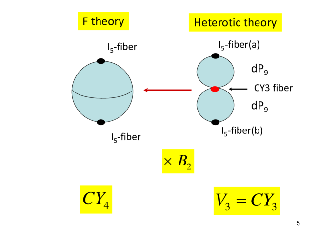
Figure 1: Heterotic to F-theory duality

2.2 F-theory side

We construct a CY4 which is defined by an elliptic fiber over a base $B_{3}$ with two sections. It is mathematically defined by a Tate form (or Weierstrass function)

$$wy^{2}=x^{3}+a_{5}wxy+a_{4}zwx^{2}+a_{3}z^{2}w^{2}y+a_{2}z^{3}w^{2}x+a_{0}z^{5}w^{3}.$$ (1)

The Tate form represents the parameters of the Higgs vector bundle which breaks $E_{8}\times E_{8}$ to a subgroup. In the Tate form the $[w,x,y]$ are the coordinates of the elliptic fiber. $z=0$ is the position where the Weierstrass descriminant vanishes and defines the GUT surface, $S_{GUT}$. Finally, $z,a_{j}$ are functions on $B_{3}$. The fiber has two sections. The first is given by

$$\zeta(b_{3})=\{[w,x,y]=[0,0,1]\}.$$ (2)

We choose the constraint

$$a_{5}+a_{4}+a_{3}+a_{2}+a_{0}=0.$$ (3)

This gives the second section

$$\tau(b_{3})=\{[w,x,y]=[1,z^{2},z^{3}]\}.$$ (4)

Now to understand the consequence of this choice, let $w=1,x=t^{2},y=t^{3}$ and define $s=z/t$. We then have

$$C\equiv a_{5}+a_{4}s+a_{3}s^{2}+a_{2}s^{3}+a_{0}s^{5}$$ (5)

which defines the spectral cover. We can also see that

$$C=(a_{5}+a_{54}s-a_{20}s^{2}-a_{0}s^{3}-a_{0}s^{4})(1-s)$$ (6)

where $a_{ij}\equiv a_{i}+a_{j}$. This gives a 4 + 1 split of the spectral cover.

2.3 The Model

Let me just give some properties of the model without any proof. For a proof one should look at the references given in the beginning.

• The model explicitly satisfies Heterotic-F-theory duality.

• On the Heterotic side there is $E_{8}\times E_{8}$ broken to the gauge group $(SU(5)\times U(1)_{X})^{2}$. On the F-theory side, as a consequence of the 4 + 1 split of the spectral cover, the Higgs bundle, $[SU(4)\times U(1)_{X}]$, lives on a 4 sheeted cover of the GUT surface. The $U(1)_{X}$ is a consequence of the 4 + 1 split of the spectral cover.

• There is a freely acting $\mathbb{Z}_{2}$ involution acting on the GUT surface. Downstairs we obtain $S_{GUT}=Enriques$.

• The gauge group $SU(5)\times U(1)_{X}$ is broken to the $SU(3)\times SU(2)\times U(1)_{Y}\times U(1)_{X}$ gauge group with Wilson line breakiing.

• There are NO vector-like exotics, since the involution includes a translation by $\zeta(b_{3})-\tau(b_{3})$.

• The model has an R-parity and a $\mathbb{Z}_{4}^{R}$ symmetry which prevents both dimension 4 and 5 baryon and lepton number violating operators.

Spectrum

The model has a visible sector with 3 families of quarks and leptons and one Higgs pair. The matter curves live on the GUT surface. The $U(1)_{X}$ charges of the matter fields are given by the superscripts

$$10^{-1}_{m},\;\bar{5}^{+3}_{m},\;5^{+2}_{h}+\bar{5}^{-2}_{h}$$ (7)

which allows for Yukawa couplings

$$10_{m}\bar{5}^{m}\bar{5}^{h},\;10_{m}10_{m}5_{h}\;\;\rm{but\;NOT}\;\;10_{m}\bar{5}_{m}\bar{5}_{m}.$$ (8)

Downstairs, after the involution, the $z=0$ is a two sheeted cover of the GUT surface. As a consequence the model includes a twin sector whose spectrum is identical to the visible sector.

The model contains right-handed [RH] neutrinos, see Ref.  [22]. The RH neutrino curve, $\Gamma^{-5}\equiv N^{-5}_{m}$, lives in $B_{3}$ along with one other curve, $\Lambda^{+10}\equiv\Phi^{+10}$. This allows for the possible Yukawa couplings

$$N^{-5}_{m}\bar{5}^{+3}_{m}5^{+2}_{h},$$ (9)

i.e. Dirac neutrino masses and

$$N^{-5}_{m}N^{-5}_{m}\Phi^{+10}.$$ (10)

Note, under the involution, $U(1)_{X}$ is broken to $\mathbb{Z}_{2}$ matter parity. Moreover, if $\Phi^{+10}$ obtains a VEV this gives a Majorana mass to the RH neutrinos.

Relative scales of the visible and twin (hidden) sectors, Ref.  [7]

In the Heterotic limit of the theory we obtain the gravity action and two gauge actions. See fig. 2.

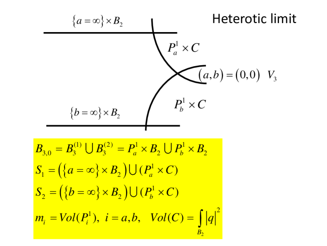
Figure 2: In the Heterotic limit the two gauge sectors separate. The parameter $\delta$ ranges from 0 to 1 where $\delta=0$ is the F-theory limit and $\delta=1$ is the Heterotic limit. The figure describes the $dP_{9}\bigcup dP_{9}$ which intersect on the elliptic curve. $V_{3}=CY3$.

The gravity action is given by

$$S_{EH}\sim M_{*}^{8}\int_{\mathbb{R}^{3,1}\times B_{3}}R\sqrt{-g_{\delta}}d^{10}x$$ (11)

with $M_{Pl}^{2}\simeq M_{*}^{8}\cdot Vol(B_{3,\delta})$. While the gauge action is given by

$$S_{gauge}\sim-M_{*}^{4}\int_{\mathbb{R}_{3,1}\times S_{i}}\left(Tr(F_{1}^{2})\sqrt{-g_{1}}+Tr(F_{2}^{2})\sqrt{-g_{2}}\right)\delta^{2}(z_{0})d^{10}x.$$ (12)

We have two gauge groups in the Heterotic limit.

We have

$$\alpha_{G}^{-1}(i)\sim M_{*}^{4}Vol(S_{i})$$ (13)

and

$$M_{G}(i)^{-4}\sim Vol(S_{i})$$ (14)

where

$$Vol(S_{i})=Vol(B_{2})+m_{i}Vol(C),\;\;m_{i}=Vol(P^{1}_{i}),\;i=a,b\equiv 1,2.$$ (15)

Thus

$$\alpha_{G}(i)M_{Pl}=\sqrt{\frac{(m_{1}+m_{2})Vol(B_{2})}{Vol(B_{2})(1+Km_{i})}}.$$ (16)

We have

$$\alpha_{G}(2)/\alpha_{G}(1)=\frac{1+Km_{1}}{1+Km_{2}},\;\;M_{G}(2)/M_{G}(1)=\left(\frac{1+Km_{1}}{1+Km_{2}}\right)^{1/4}.$$ (17)

For example if we take for the visible sector $\alpha_{G}(1)^{-1}=24,\,M_{G}(1)=3\times 10^{16}$ GeV and for the twin sector, take $\alpha_{G}(2)^{-1}=8.7,\,M_{G}(1)=3.9\times 10^{16}$ GeV we need $\frac{1+Km_{1}}{1+Km_{2}}=2.8$.

Summary

• We constructed a Global $SU(5)$ F-theory model with Wilson line breaking.

• The Wilson line wraps the GUT surface breaking $SU(5)$ to the SM gauge group.

• It has a complete twin sector with different scales determined by the sizes of the visible and twin manifolds.

• $M_{GUT}=M_{compactification}\sim 1/R_{cycle}$

• Non-local GUT breaking by the Wilson line gives precise gauge coupling unification.

• It contains 3 families and one pair of Higgs doublets and NO vector-like exotics !

• It has a $\mathbb{Z}_{2}$ matter parity and a $\mathbb{Z}_{4}^{R}$ symmetry.

• Allowed Yukawa couplings are consistent with what is needed for giving quarks and charged lepton masses and a See-Saw mechanism for neutrino masses.

• Twin matter contains a dark matter candidate ?

2.4 Neutrino Portal

The Low Energy Theory

We have the MSSM and a twin MSSM^′. We assume $\Lambda_{QCD^{\prime}}>\Lambda_{QCD}$ which implies heavier twin baryons. In both the visible and twin sectors there are two pairs of Higgs doublets. We assume the VEVs in the twin sector

$$\langle H_{u}^{\prime}\rangle=\left(\begin{array}[]{c}0\\ v_{H_{u}^{\prime}}\end{array}\right),\;\;\;\;\langle H_{d}^{\prime}\rangle=\left(\begin{array}[]{c}v_{H_{d}^{\prime}}\\ 0\end{array}\right).$$ (18)

We also assume, generically, $v_{H^{\prime}}>v_{H}$ which implies heavier twin Dirac quark and lepton masses. RH neutrino masses are given by

$$y_{ij}\langle\Phi\rangle\Gamma_{i}\Gamma_{j}\Rightarrow M_{ij}N_{i}N_{j},\;\;i,j=1,..,,3.$$ (19)

They are identified in the visible and twin sectors with one global $U(1)_{X}$.

The superpotential is given by

$$W=\frac{1}{2}N_{i}M_{ij}N_{j}+N_{i}Y_{ij}\ell_{j}H_{u}+N_{i}Y_{ij}^{\prime}\ell^{\prime}_{j}H^{\prime}_{u},$$ (20)

where $\ell_{i}$ and $H_{u}$ ($\ell_{i}^{\prime}$ and $H_{u}^{\prime}$) are the MSSM (twin) lepton and up-type Higgs doublets.

After integrating out the heavy neutrinos (assuming $M\gg v_{H}^{\prime}>v_{H}$) we have

$$W=-\frac{1}{2}(\ell Y^{T}H_{u}+\ell^{\prime}Y^{\prime T}H_{u}^{\prime})M^{-1}(Y\ell H_{u}+Y^{\prime}\ell^{\prime}H^{\prime}_{u}).$$ (21)

Clearly there are 3 massive and 3 massless neutrinos.

Radiative neutrino masses, Ref.  [23]

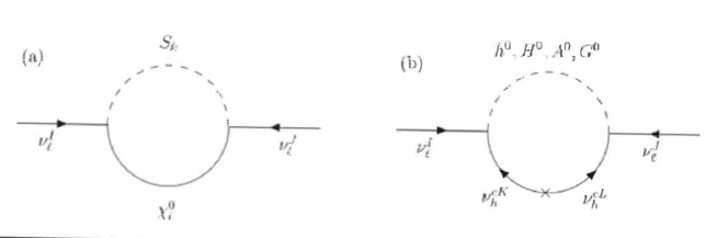
Figure 3: In these one loop diagrams, (a) $S_{k}(k=1,...,6)$ are the light sneutrinos and $\chi_{i}^{0}$ are neutralinos. (b) These include Higgs, goldstinos and heavy neutrinos.

The light neutrino masses, including radiative corrections, are given by

$$M_{\nu_{\ell}}=\left(\begin{pmatrix}\delta m_{LL}-m_{D}^{T}M^{-1}m_{D}&-m_{D}^{T}M^{-1}m_{D^{\prime}}\\ -m_{D^{\prime}}^{T}M^{-1}m_{D}&\delta m_{L^{\prime}L^{\prime}}-m_{D^{\prime}}^{T}M^{-1}m_{D^{\prime}}\end{pmatrix}\right)$$ (22)

and in the limit $m_{D^{\prime}}\gg m_{D}$ we have

$$M_{\nu_{\ell}}\sim\left(\begin{pmatrix}\delta m_{LL}&0\\ 0&-m_{D^{\prime}}^{T}M^{-1}m_{D^{\prime}}\end{pmatrix}\right).$$ (23)

We define the diagonalization unitary matrix $U_{\ell}$ for the light neutrino mass matrix with radiative corrections as

$$U_{\ell}^{T}M_{\nu_{\ell}}U_{\ell}=\mathrm{diag}\left(m_{\nu_{1}},m_{\nu_{2}},m_{\nu_{3}},m_{\nu_{4}},m_{\nu_{5}},m_{\nu_{6}}\right),$$ (24)

We decompose $U_{\ell}$ and parametrize the upper $3\times 6$ block of it as

$$U_{\ell}=:\begin{pmatrix}A_{\ell}\\ A_{\ell^{\prime}}\end{pmatrix},\quad A_{\ell}=:\begin{pmatrix}U_{e1}&U_{e2}&U_{e3}&U_{e4}&U_{e5}&U_{e6}\\ U_{\mu 1}&U_{\mu 2}&U_{\mu 3}&U_{\mu 4}&U_{\mu 5}&U_{\mu 6}\\ U_{\tau 1}&U_{\tau 2}&U_{\tau 3}&U_{\tau 4}&U_{\tau 5}&U_{\tau 6}\\ \end{pmatrix},$$ (25)

where the left (right) three columns of $A_{\ell}$ are for the active (sterile) neutrinos.

The $W$ boson coupling is given by

$$\mathcal{L}_{W}=\frac{g}{\sqrt{2}}W_{\mu}^{-}\overline{\psi}_{e}\gamma^{\mu}P_{L}A_{\ell}\Psi_{\ell}+h.c.,$$ (26)

where $\Psi_{\ell}$ contains the neutrinos in the mass basis without the heaviest three states with $\mathcal{O}\left({M}\right)$ masses. Here, we choose the flavor basis that the charged lepton Yukawa matrix is positive diagonal in the gauge basis. We assume that the Pontecorvo-Maki-Nakagawa-Sakata (PMNS) matrix for the active neutrinos are almost unitary, so that the angles in the standard parametrization,

$$U_{\mathrm{PMNS}}=\begin{pmatrix}1&0&0\\ 0&c_{23}&s_{23}\\ 0&-s_{23}&c_{23}\\ \end{pmatrix}\begin{pmatrix}c_{13}&0&s_{13}e^{-i\delta}\\ 0&1&0\\ -s_{13}e^{i\delta}&0&c_{13}\\ \end{pmatrix}\begin{pmatrix}c_{12}&s_{12}&0\\ -s_{12}&c_{12}&0\\ 0&0&1\end{pmatrix},$$ (27)

are related to the elements in $A_{\ell}$ as

$$s_{12}=\frac{\left|{U_{e2}}\right|}{\sqrt{\left|{U_{e1}}\right|^{2}+\left|{U_{e2}}\right|^{2}}}\quad s_{23}=\frac{\left|{U_{\mu 3}}\right|}{\sqrt{\left|{U_{\mu 3}}\right|^{2}+\left|{U_{\tau 3}}\right|^{2}}}\quad s_{13}=\left|{U_{e3}}\right|,$$ (28)

and

$$e^{i\delta}=\left|{\frac{U_{e2}U_{e3}U_{\mu 3}}{U_{e1}U_{\tau 3}}}\right|\left(1+\frac{\sqrt{\left|{U_{e1}}\right|^{2}+\left|{U_{e2}}\right|^{2}}\sqrt{\left|{U_{\tau 3}}\right|^{2}+\left|{U_{\mu 3}}\right|^{2}}}{\left|{U_{\mu 3}}\right|^{2}}\frac{U_{\mu 2}^{*}U_{\mu 3}}{U_{e2}^{*}U_{e3}}\right).$$ (29)

Here, we consider the fitted data with the normal ordering (NO) [24, 25]:

$$\Delta m_{12}^{2}=(7.55\pm 0.20)\times 10^{-5}~{}\mathrm{eV},\quad\Delta m_{23}^{2}=(2.424\pm 0.030)\times 10^{-3}~{}\mathrm{eV},$$ (30)

$$s_{12}^{2}=0.32\pm 0.02,\quad s_{23}^{2}=0.547\pm 0.03,\quad s_{13}^{2}=0.0216\pm 0.0083,\quad\delta_{\mathrm{CP}}=218\pm 38~{}\mathrm{deg},$$ (31)

and with the inverted ordering (IO) [24, 25]:

$$\Delta m_{12}^{2}=(7.55\pm 0.20)\times 10^{-5}~{}\mathrm{eV},\quad\Delta m_{23}^{2}=(-2.50\pm 0.040)\times 10^{-3}~{}\mathrm{eV},$$ (32)

$$s_{12}^{2}=0.32\pm 0.02,\quad s_{23}^{2}=0.5551\pm 0.03,\quad s_{13}^{2}=0.0220\pm 0.0076,\quad\delta_{\mathrm{CP}}=281\pm 27~{}\mathrm{deg},$$ (33)

where $\Delta m_{ij}^{2}:=m_{\nu_{j}}^{2}-m_{\nu_{i}}^{2}$. For reference, typical values of the absolute values of the PMNS matrix is

$$\left|{U_{\mathrm{PMNS}}}\right|\sim\begin{pmatrix}0.82&0.55&0.15\\ 0.31&0.60&0.74\\ 0.48&0.58&0.66\end{pmatrix}.$$ (34)

In our notation, the lightest neutrino is $\nu_{1}$ ($\nu_{3}$) for the NO (IO) case, but the sterile neutrinos are ordered by their masses, so the lightest sterile neutrino is always $\nu_{4}$.

The Majorana neutrinos can induce neutrino-less double $\beta$ (${0\nu\beta\beta}$) decay. The ${0\nu\beta\beta}$ decay half-life is given by [26],

$$\left[T^{0\nu}_{1/2}\right]^{-1}=\mathcal{A}\left|{m_{p}\sum_{i=1}^{6}U^{2}_{ei}\frac{m_{\nu_{i}}}{\langle{p^{2}}\rangle+m_{\nu_{i}}^{2}}}\right|^{2},$$ (35)

where the values of $\mathcal{A}$ and $\langle{p^{2}}\rangle\simeq(200~{}\mathrm{MeV})^{2}$ are tabulated in Table.1 of Ref. [26]. We choose the values which provide the most conservative limits, i.e. (a) Argonne potential with $g_{A}=1.00$, for $\langle{p^{2}}\rangle$ and $\mathcal{A}$; $\sqrt{\langle{p^{2}}\rangle}(^{76}\mathrm{Ge})=0.159~{}\mathrm{GeV}$, $\mathcal{A}(^{76}\mathrm{Ge})=2.55\times 10^{-10}\;\mathrm{yrs}^{-1}$, and $\sqrt{\langle{p^{2}}\rangle}(^{136}\mathrm{Xe})=0.178~{}\mathrm{GeV}$, $\mathcal{A}(^{136}\mathrm{Xe})=4.41\times 10^{-10}\;\mathrm{yrs}^{-1}$. The limits for ⁷⁶Ge and ¹³⁶Xe are [27, 28]

$$T_{1/2}^{0\nu}(^{76}\mathrm{Ge})\geq 3.0\times 10^{25}~{}\mathrm{years},\quad T_{1/2}^{0\nu}(^{136}\mathrm{Xe})\geq 3.4\times 10^{25}~{}\mathrm{years},$$ (36)

respectively.

2.5 Simplified analysis

For simplicy we assume $Y^{\prime}=Y,\;\;v_{H}<v^{\prime}_{H},$ the Majorana mass, $M$ and the Yukawa matrices, $Y^{\prime}_{e}=Y_{e}$, are diagonal with positive elements. We consider $m_{H},m_{A}\gg m_{h}$ i.e. the decoupling limit and $\tan\beta^{\prime}\neq\tan\beta,\;\;M_{N}=10^{12}$  GeV. We consider the CMSSM scenario for soft parameters with $\tan\beta=10,\;\;\sin\mu=+1,\;\;m_{0}=-A_{0}=5$ TeV. and $M_{1/2}=2.5$ TeV. We calculate the parameters at the TeV scale by using softsusy-4.1.12 [29]. At this point, the SM-like Higgs mass is $125.69~{}\mathrm{GeV}$. The soft parameters relevant to the neutrino masses are given by

$$M_{1}=1.134~{}\mathrm{TeV},\quad M_{2}=2.017~{}\mathrm{TeV},\quad\mu=3.424~{}\mathrm{TeV},$$ (37)

$$\quad m_{L}=(5.2269,5.2268,5.1983)~{}\mathrm{TeV}.$$ (38)

The lightest neutrino, $\nu_{1}$ for NO and $\nu_{3}$ for IO, mass is assumed to be $0.001~{}\mathrm{eV}$. We scan over the value of $v_{H^{\prime}}/v_{H}$. We always found the values which explain the neutrino mixing parameters throughout our scan, up to numerical errors.

The left panel of Fig. 4 shows the mass and mixing of the lightest sterile neutrino $\nu_{4}$. The solid (dashed) lines are the cases of NO (IO) of the active neutrinos. Since we assume $m_{D}\propto m_{D^{\prime}}$, the mixing matrix for the sterile neutrinos are similar to the active ones up to the $\mathcal{O}\left({1}\right)$ coefficients from the soft parameters, i.e.

$$\begin{pmatrix}\left|{U_{e4}}\right|\\ \left|{U_{\mu 4}}\right|\\ \left|{U_{\tau 4}}\right|\end{pmatrix}\propto\begin{pmatrix}\left|{U_{e1}}\right|\\ \left|{U_{\mu 1}}\right|\\ \left|{U_{\tau 1}}\right|\end{pmatrix}~{}\mathrm{for~{}NO\quad and}~{}\begin{pmatrix}\left|{U_{e4}}\right|\\ \left|{U_{\mu 4}}\right|\\ \left|{U_{\tau 4}}\right|\end{pmatrix}\propto\begin{pmatrix}\left|{U_{e3}}\right|\\ \left|{U_{\mu 3}}\right|\\ \left|{U_{\tau 3}}\right|\end{pmatrix}~{}\mathrm{for~{}IO}.$$ (39)

Thus, $\left|{U_{e4}}\right|$ ($\left|{U_{\mu 4}}\right|$) is the largest element in the NO (IO) case.

The right panel of Fig. 4 shows the lifetime of ${0\nu\beta\beta}$ decays. Since the sterile neutrinos are much lighter than $\mathcal{O}\left({100~{}\mathrm{MeV}}\right)$ for $v_{H^{\prime}}/v_{H}\lesssim 10^{4}$, the contributions are proportional to $U_{ei}^{2}m_{\nu_{i}}$. In the NO case, the contributions from the heavier sterile neutrinos are more suppressed by the mixing angles, see Eq. (34). While in the IO case, the heavier states have degenerate masses, $m_{\nu_{5}}\simeq m_{\nu_{6}}$ and the mixing angles are not suppressed. Therefore the lifetimes are much shorter for the IO case, and hence $m_{\nu_{1}}\lesssim 0.001~{}\mathrm{eV}$ is required to be consistent with the current limits.

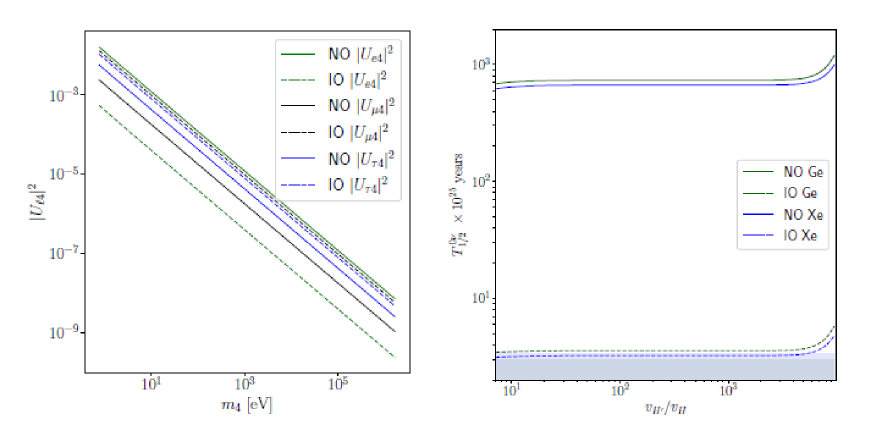
Figure 4: The mass and mixing of the lightest sterile neutrino $\nu_{4}$ (left) and the $0\nu\beta\beta$ decay with varying $v_{H^{\prime}}/v_{H}$ (right). On the left panel, the solid (dashed) lines correspond to the NO (IO). The colors are the charged lepton flavors. On the right panel, the green (blue) lines are the values for Ge (Xe). The colored regions are the lower bounds on the lifetime.

Table 1 shows the benchmark points in the NO and IO cases. The size of $v_{H^{\prime}}/v_{H}$ is chosen such that the anomaly in the reactor experiments, discussed in the next section, are explained in the NO case. We see that the neutrino mixing data is consistent with the neutrino mixing observables. The mixing angles involving the sterile neutrinos are much smaller than those in the active neutrinos, and hence the $3\times 3$ PMNS matrix is almost unitary. Since we assume the flavor structure of the Dirac matrices are the same, the relative sizes of the masses and mixing are similar among the active and sterile neutrinos. The lifetime of the eV sterile neutrinos are longer than $10^{35}~{}\mathrm{sec}$ [30, 31, 32, 33], so the sterile neutrinos are stable as compared to the age of the universe.

Table 1: The benchmark points in the CMSSM scenario.

	NO	IO
$\log_{10}v_{H^{\prime}}/v_{H}$	0.89	0.89
$(d_{1},d_{2},d_{3})~{}[\mathrm{eV}]$	(0.0185, -0.1621, 0.9270)	(-0.9129, 0.9271, 0.0185)
$(s_{12}^{n},s_{23}^{n},s_{13}^{n},\delta_{n})$	(0.3680, 0.7051, 0.5073, 0.3436)	(0.4601, 0.7575, 0.4231, 0.5122)
$(\Delta m_{12}^{2}\times 10^{5},\Delta m_{23}^{2}\times 10^{3})~{}[\mathrm{eV}^{2}]$	(7.550, 2.424)	(7.550, -2.500)
$(s_{12}^{2},s_{23}^{2},s_{13}^{2},\delta)$	(0.320, 0.547, 0.022, -2.478)	(0.320, 0.551, 0.022, -1.379)
$(m_{\nu_{4}},m_{\nu_{5}},m_{\nu_{6}})$ [eV]	(1.136, 9.932, 56.784)	(1.136, 55.923, 56.789)
$\left|\begin{pmatrix}U_{e4}&U_{e5}&U_{e6}\\ U_{\mu 4}&U_{\mu 5}&U_{\mu 6}\\ U_{\tau 4}&U_{\tau 5}&U_{\tau 6}\end{pmatrix}\right|$	$\begin{pmatrix}0.1041&0.0714&0.0189\\ 0.0401&0.0772&0.0934\\ 0.0620&0.0723&0.0850\\ \end{pmatrix}$	$\begin{pmatrix}0.0191&0.1043&0.0711\\ 0.0937&0.0517&0.0696\\ 0.0846&0.0524&0.0800\\ \end{pmatrix}$
$(T^{0\nu}_{1/2}(^{76}\mathrm{Ge}),T^{0\nu}_{1/2}(^{136}\mathrm{Xe}))$ years	$(689.99,626.67)\times 10^{25}$	$(3.46,3.14)\times 10^{25}$

2.6 Sterile neutrino phenomenology

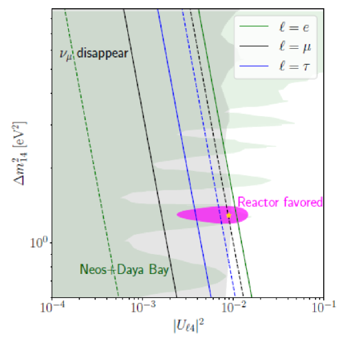
Figure 5: The mixing angle vs $\Delta m_{14}^{2}:=m_{4}^{2}-m_{1}^{2}$. The green, black and blue lines are $\ell=e,\mu$ and $\tau$, respectively. The solid (dashed) lines are normal (inverse) hierarchy. The green (gray) region is allowed by the Neos$+$Daya ($\nu_{\mu}$ disappearance). The combined $\nu_{e}$ disappearance result favors the magenta region. The yellow star is the best-fit point in the analysis of Ref. [34].

We study the phenomenology of neutrino mixing with the lightest sterile neutrino $\nu_{4}$, see Refs. [35, 36] for recent reviews of sterile neutrinos. Under the assumption of $m_{D^{\prime}}\propto m_{D}$, the heavier state $\nu_{5}$ is about 8 (50) times heavier than $\nu_{4}$ in the NO (IO), and hence the mixing with these will be sub-dominant . The following combinations of the mixing with $\nu_{4}$ are constrained from the reactor experiments [34],

• $\nu_{e}$ disappearance $\propto|U_{e4}|^{2}$ [39, 40, 41]

• $\nu_{\mu}\to\nu_{e}$ oscillations at short baseline $\propto|U_{e4}U_{\mu 4}|^{2}$ [42, 43, 44, 45, 46, 47]

• $\nu_{\mu}$ disappearance, $\propto|U_{\mu 4}|^{2}$ [48, 49, 50, 51, 52, 53, 54, 55]

The limit for $\left|{U_{\tau 4}}\right|^{2}<0.13$ [34] is much weaker than limits on the above combinations [50, 51]. In the reactor experiments measuring the $\nu_{e}$ disappearance, DayaBay and NEOS put upper bounds on $\left|{U_{e4}}\right|^{2}$ [39, 40], but the DANSS reported an excess [41]. It is interesting that the excess can be explained consistently with the limits from DayaBay+NEOS, where $\Delta m_{14}^{2}=1.29~{}\mathrm{eV}^{2}$ and $\left|{U_{e4}}\right|^{2}=0.0089$ [34]. Anomalies are found in the short base-line experiments LSND [42] and MiniBooNE [43], which favor $\Delta m_{14}^{2}\sim 0.5~{}\mathrm{eV}^{2}$ and $4|U_{e4}U_{\mu 4}|^{2}\sim 0.007$. The $\nu_{\mu}$ measurements, however, exclude $|U_{\mu 4}|^{2}\lesssim 0.01$ for $\Delta m_{14}^{2}\sim\mathcal{O}\left({0.1-10~{}\mathrm{eV}^{2}}\right)$, and therefore the explanation of the short base-line anomalies by the mixing with a sterile neutrino is excluded by the $\nu_{\mu}$ disappearance result [34]. Hence we do not consider the anomalies in the short base-line experiments.

Figure 5 shows the favored regions by the experiments searching for the mixing with a sterile neutrino. The green (gray) region is allowed by the Neos+Daya Bay ($\nu_{\mu}$ disappearance) result, which should be compared with the green (black) lines. The pink region is the favored region from all the reactor data, including the DANSS result which observed the anomaly. In the NO case, the green solid line overlaps the pink region, and the black line is inside the gray region. Thus, the anomaly in the DANSS experiment can be explained in this case. The benchmark point for the NO case in Table 1 is chosen from the overlapped region. In the IO case, however, the mixing with electron $\left|{U_{e4}}\right|$ is much smaller than the value preferred by the reactor data for $\Delta m_{14}^{2}\sim 1~{}\mathrm{eV}$. Furthermore, this case will be excluded by the $\nu_{\mu}$ disappearance result even if $\left|{U_{e4}}\right|$ has a certain value because $\left|{U_{e4}}\right|<\left|{U_{\mu 4}}\right|$. Therefore, the reactor data is fully explained only in the NO case.

2.7 Cosmology

The $\mathrm{eV}$ sterile neutrinos which can explain the reactor anomaly may, however, be incompatible with cosmological observations [36]. The Planck collaboration obtained the $95\%$ C.L. upper limits on the effective number of neutrinos $N_{\mathrm{eff}}<3.29$ and the sum of the neutrino masses $\sum m_{\nu}<0.65~{}\mathrm{eV}$ [56]. This may have several different types of solutions which I will not get into here.

Before closing, we briefly discuss the cosmology of the other particles in the twin sector. The twin photon may contribute to $N_{\mathrm{eff}}$ along with the light sterile neutrinos. The contribution could be suppressed if the temperature of the thermal bath of the twin sector is significantly smaller than the MSSM one. This requires that the reheating process occurs predominantly in the MSSM sector. Another possibility is that the twin photon is massive due to the non-zero VEV of the charged Higgs or sparticles. This would be the case, for instance, if anomaly mediation [57, 58] is the dominant source for SUSY breaking in the twin sector. In our model, the photon to twin photon kinetic mixing, $\epsilon F^{\mu\nu}F^{\prime}_{\mu\nu}$, where $F_{\mu\nu}$ ($F^{\prime}_{\mu\nu}$) is the field strength of the (twin) photon, is expected to be tiny. There is a 3-loop diagram which is mediated by neutrinos whose order is estimated as

$$\epsilon\sim\frac{g^{3}g^{\prime 3}m_{\nu^{\prime}}^{2}}{(16\pi^{2})^{3}m_{W}m_{W^{\prime}}}\sim 10^{-25}\times\left(\frac{\sqrt{gg^{\prime}}}{0.5}\right)^{6}\left(\frac{m_{\nu^{\prime}}}{50~{}\mathrm{eV}}\right)^{2}\frac{m_{W}}{m_{W^{\prime}}}.$$ (40)

Therefore it is negligibly small.

The twin electrons and baryons are stable and can contribute to the DM density. If the asymmetry of the twin particles and anti-particles are negligible, the twin particles annihilate when they freeze-out from the twin thermal bath. While the twin particles become the asymmetric DM if the asymmetry is non-negligible also in the twin sector. Thus the abundance of the twin fermions will be small if the annihilation is large or the asymmetry is small.

The lightest SUSY particle (LSP) in the twin sector may also be stable due to R-parity in the same way as the LSP in the MSSM. If $m_{\mathrm{tLSP}}>m_{3/2}$, the twin LSP (tLSP) can decay to the gravitino plus the SUSY partner of the tLSP, or to the MSSM sparticle through the gravitino, depending on the mass spectrum. For example, the tLSP can decay to a gravitino via the processes ${\tilde{\nu}}^{\prime}\to\nu^{\prime}\psi_{3/2}$ or $\widetilde{B}^{\prime}\to\gamma^{\prime}\psi_{3/2}$ as long as it is kinematically allowed. The gravitino can then decay to the LSP in the MSSM. Here we assume that the $m_{\mathrm{tLSP}}>m_{3/2}>m_{\mathrm{LSP}}$. In this case, the twin LSP should be heavier than the TeV scale, so that the twin LSP/gravitino decay does not alter the success of Big Bang Nucleosynthesis (BBN).

2.8 Summary

• We studied the neutrino sector in a global $SU(5)$ F theory GUT.

• $SU(5)$ is spontaneously broken to the SM gauge symmetry via a Wilson line.

• At low energies the model has the MSSM spectrum with a complete MSSM^′ twin sector.

• The right-handed neutrinos in the visible and twin sectors are identified.

• Assuming 3 right-handed neutrinos which get a Majorana mass at a scale of order $10^{12}$ GeV, we analyzed the light neutrino spectrum.

• Three predominantly sterile neutrinos get mass via the See-Saw mechanism at tree level.

• The other three predominantly active neutrinos obtain mass via radiative corrections.

• We fit the light neutrino masses to data.

• Questions of cosmology are saved for the future.

References

- [1] J. Kawamura and S. Raby, A Right-handed neutrino portal to the hidden sector: active neutrinos and their twins in an F-theory model, JHEP 02 (2023) 239, [arXiv:2212.00840].
- [2] H. Clemens and S. Raby, Heterotic--theory Duality with Wilson Line Symmetry-breaking, JHEP 12 (2019) 016, [arXiv:1908.01913].
- [3] H. Clemens and S. Raby, Heterotic/-theory Duality and Narasimhan-Seshadri Equivalence, arXiv:1906.07238.
- [4] H. Clemens and S. Raby, F-theory over a Fano threefold built from -roots, arXiv:1908.01110.
- [5] R. Donagi and M. Wijnholt, Model Building with F-Theory, Adv. Theor. Math. Phys. 15 (2011), no. 5 1237–1317, [arXiv:0802.2969].
- [6] C. Beasley, J. J. Heckman, and C. Vafa, GUTs and Exceptional Branes in F-theory - II: Experimental Predictions, JHEP 01 (2009) 059, [arXiv:0806.0102].
- [7] C. H. Clemens and S. Raby, Relative Scales of the GUT and Twin Sectors in an F-theory model, JHEP 04 (2020) 004, [arXiv:2001.10047].
- [8] K. S. Babu and R. N. Mohapatra, Solution to the strong problem without an axion, Phys. Rev. D 41 (Feb, 1990) 1286–1291.
- [9] S. M. Barr, D. Chang, and G. Senjanovic, Strong CP problem and parity, Phys. Rev. Lett. 67 (1991) 2765–2768.
- [10] P.-H. Gu, A left-right symmetric model with SU(2)-triplet fermions, Phys. Rev. D 84 (2011) 097301, [arXiv:1110.6049].
- [11] P.-H. Gu, Mirror left-right symmetry, Phys. Lett. B 713 (2012) 485–489, [arXiv:1201.3551].
- [12] P.-H. Gu, Mirror symmetry: from active and sterile neutrino masses to baryonic and dark matter asymmetries, Nucl. Phys. B 874 (2013) 158–176, [arXiv:1303.6545].
- [13] G. Abbas, A low scale left-right symmetric mirror model, Mod. Phys. Lett. A 34 (2019), no. 15 1950119, [arXiv:1706.01052].
- [14] G. Abbas, A model of spontaneous breaking at low scale, Phys. Lett. B 773 (2017) 252–257, [arXiv:1706.02564].
- [15] P.-H. Gu, Spontaneous mirror left-right symmetry breaking for leptogenesis parametrized by Majorana neutrino mass matrix, JHEP 10 (2017) 016, [arXiv:1706.07706].
- [16] L. J. Hall and K. Harigaya, Implications of Higgs Discovery for the Strong CP Problem and Unification, JHEP 10 (2018) 130, [arXiv:1803.08119].
- [17] J. Kawamura, S. Okawa, Y. Omura, and Y. Tang, WIMP dark matter in the parity solution to the strong CP problem, JHEP 04 (2019) 162, [arXiv:1812.07004].
- [18] D. Dunsky, L. J. Hall, and K. Harigaya, Higgs Parity, Strong CP, and Dark Matter, JHEP 07 (2019) 016, [arXiv:1902.07726].
- [19] M. Berbig, The Type II Dirac Seesaw Portal to the mirror sector: Connecting neutrino masses and a solution to the strong CP problem, arXiv:2209.14246.
- [20] Y. Zhang, X. Ji, and R. N. Mohapatra, A Naturally Light Sterile neutrino in an Asymmetric Dark Matter Model, JHEP 10 (2013) 104, [arXiv:1307.6178].
- [21] H. An, S.-L. Chen, R. N. Mohapatra, and Y. Zhang, Leptogenesis as a Common Origin for Matter and Dark Matter, JHEP 03 (2010) 124, [arXiv:0911.4463].
- [22] C. H. Clemens and S. Raby, Right-handed neutrinos and symmetry-breaking, JHEP 04 (2020) 059, [arXiv:1912.06902].
- [23] A. Dedes, H. E. Haber, and J. Rosiek, Seesaw mechanism in the sneutrino sector and its consequences, JHEP 11 (2007) 059, [arXiv:0707.3718].
- [24] P. F. de Salas, D. V. Forero, C. A. Ternes, M. Tortola, and J. W. F. Valle, Status of neutrino oscillations 2018: 3 hint for normal mass ordering and improved CP sensitivity, Phys. Lett. B 782 (2018) 633–640, [arXiv:1708.01186].
- [25] Particle Data Group Collaboration, R. L. Workman et al., Review of Particle Physics, PTEP 2022 (2022) 083C01.
- [26] A. Faessler, M. González, S. Kovalenko, and F. Šimkovic, Arbitrary mass Majorana neutrinos in neutrinoless double beta decay, Phys. Rev. D 90 (2014), no. 9 096010, [arXiv:1408.6077].
- [27] KamLAND-Zen Collaboration, A. Gando et al., Limit on Neutrinoless Decay of 136Xe from the First Phase of KamLAND-Zen and Comparison with the Positive Claim in 76Ge, Phys. Rev. Lett. 110 (2013), no. 6 062502, [arXiv:1211.3863].
- [28] GERDA Collaboration, M. Agostini et al., Results on Neutrinoless Double- Decay of 76Ge from Phase I of the GERDA Experiment, Phys. Rev. Lett. 111 (2013), no. 12 122503, [arXiv:1307.4720].
- [29] B. C. Allanach, SOFTSUSY: a program for calculating supersymmetric spectra, Comput. Phys. Commun. 143 (2002) 305–331, [hep-ph/0104145].
- [30] B. W. Lee and R. E. Shrock, Natural Suppression of Symmetry Violation in Gauge Theories: Muon - Lepton and Electron Lepton Number Nonconservation, Phys. Rev. D 16 (1977) 1444.
- [31] P. B. Pal and L. Wolfenstein, Radiative Decays of Massive Neutrinos, Phys. Rev. D 25 (1982) 766.
- [32] V. D. Barger, R. J. N. Phillips, and S. Sarkar, Remarks on the KARMEN anomaly, Phys. Lett. B 352 (1995) 365–371, [hep-ph/9503295]. [Erratum: Phys.Lett.B 356, 617–617 (1995)].
- [33] M. Drewes et al., A White Paper on keV Sterile Neutrino Dark Matter, JCAP 01 (2017) 025, [arXiv:1602.04816].
- [34] M. Dentler, A. Hernández-Cabezudo, J. Kopp, P. A. N. Machado, M. Maltoni, I. Martinez-Soler, and T. Schwetz, Updated Global Analysis of Neutrino Oscillations in the Presence of eV-Scale Sterile Neutrinos, JHEP 08 (2018) 010, [arXiv:1803.10661].
- [35] S. Böser, C. Buck, C. Giunti, J. Lesgourgues, L. Ludhova, S. Mertens, A. Schukraft, and M. Wurm, Status of Light Sterile Neutrino Searches, Prog. Part. Nucl. Phys. 111 (2020) 103736, [arXiv:1906.01739].
- [36] B. Dasgupta and J. Kopp, Sterile Neutrinos, Phys. Rept. 928 (2021) 1–63, [arXiv:2106.05913].
- [37] C. Giunti and M. Laveder, 3+1 and 3+2 Sterile Neutrino Fits, Phys. Rev. D 84 (2011) 073008, [arXiv:1107.1452].
- [38] D. Hollander and I. Mocioiu, Minimal 3+2 sterile neutrino model at LBNE, Phys. Rev. D 91 (2015), no. 1 013002, [arXiv:1408.1749].
- [39] Daya Bay Collaboration, F. P. An et al., Improved Search for a Light Sterile Neutrino with the Full Configuration of the Daya Bay Experiment, Phys. Rev. Lett. 117 (2016), no. 15 151802, [arXiv:1607.01174].
- [40] NEOS Collaboration, Y. J. Ko et al., Sterile Neutrino Search at the NEOS Experiment, Phys. Rev. Lett. 118 (2017), no. 12 121802, [arXiv:1610.05134].
- [41] I. Alekseev et al., DANSS: Detector of the reactor AntiNeutrino based on Solid Scintillator, JINST 11 (2016), no. 11 P11011, [arXiv:1606.02896].
- [42] LSND Collaboration, A. Aguilar-Arevalo et al., Evidence for neutrino oscillations from the observation of appearance in a beam, Phys. Rev. D 64 (2001) 112007, [hep-ex/0104049].
- [43] MiniBooNE Collaboration, A. A. Aguilar-Arevalo et al., Improved Search for Oscillations in the MiniBooNE Experiment, Phys. Rev. Lett. 110 (2013) 161801, [arXiv:1303.2588].
- [44] KARMEN Collaboration, B. Armbruster et al., Upper limits for neutrino oscillations muon-anti-neutrino — electron-anti-neutrino from muon decay at rest, Phys. Rev. D 65 (2002) 112001, [hep-ex/0203021].
- [45] NOMAD Collaboration, P. Astier et al., Search for nu(mu) — nu(e) oscillations in the NOMAD experiment, Phys. Lett. B 570 (2003) 19–31, [hep-ex/0306037].
- [46] M. Antonello et al., Experimental search for the “LSND anomaly” with the ICARUS detector in the CNGS neutrino beam, Eur. Phys. J. C 73 (2013), no. 3 2345, [arXiv:1209.0122].
- [47] OPERA Collaboration, N. Agafonova et al., Search for oscillations with the OPERA experiment in the CNGS beam, JHEP 07 (2013) 004, [arXiv:1303.3953]. [Addendum: JHEP 07, 085 (2013)].
- [48] IceCube Collaboration, M. G. Aartsen et al., Determining neutrino oscillation parameters from atmospheric muon neutrino disappearance with three years of IceCube DeepCore data, Phys. Rev. D 91 (2015), no. 7 072004, [arXiv:1410.7227].
- [49] IceCube Collaboration, M. G. Aartsen et al., Searches for Sterile Neutrinos with the IceCube Detector, Phys. Rev. Lett. 117 (2016), no. 7 071801, [arXiv:1605.01990].
- [50] MINOS+ Collaboration, P. Adamson et al., Search for sterile neutrinos in MINOS and MINOS+ using a two-detector fit, Phys. Rev. Lett. 122 (2019), no. 9 091803, [arXiv:1710.06488].
- [51] NOvA Collaboration, P. Adamson et al., Search for active-sterile neutrino mixing using neutral-current interactions in NOvA, Phys. Rev. D 96 (2017), no. 7 072006, [arXiv:1706.04592].
- [52] Super-Kamiokande Collaboration, R. Wendell et al., Atmospheric neutrino oscillation analysis with sub-leading effects in Super-Kamiokande I, II, and III, Phys. Rev. D 81 (2010) 092004, [arXiv:1002.3471].
- [53] MiniBooNE Collaboration, A. A. Aguilar-Arevalo et al., A Search for muon neutrino and antineutrino disappearance in MiniBooNE, Phys. Rev. Lett. 103 (2009) 061802, [arXiv:0903.2465].
- [54] MiniBooNE, SciBooNE Collaboration, G. Cheng et al., Dual baseline search for muon antineutrino disappearance at , Phys. Rev. D 86 (2012) 052009, [arXiv:1208.0322].
- [55] Super-Kamiokande Collaboration, R. Wendell, Atmospheric Results from Super-Kamiokande, AIP Conf. Proc. 1666 (2015), no. 1 100001, [arXiv:1412.5234].
- [56] Planck Collaboration, N. Aghanim et al., Planck 2018 results. VI. Cosmological parameters, Astron. Astrophys. 641 (2020) A6, [arXiv:1807.06209]. [Erratum: Astron.Astrophys. 652, C4 (2021)].
- [57] L. Randall and R. Sundrum, Out of this world supersymmetry breaking, Nucl. Phys. B 557 (1999) 79–118, [hep-th/9810155].
- [58] G. F. Giudice, M. A. Luty, H. Murayama, and R. Rattazzi, Gaugino mass without singlets, JHEP 12 (1998) 027, [hep-ph/9810442].