Square Root LASSO: well-posedness, Lipschitz stability and the tuning trade off

Abstract

This paper studies well-posedness and parameter sensitivity of the Square Root LASSO (SR-LASSO), an optimization model for recovering sparse solutions to linear inverse problems in finite dimension. An advantage of the SR-LASSO (e.g., over the standard LASSO) is that the optimal tuning of the regularization parameter is robust with respect to measurement noise. This paper provides three point-based regularity conditions at a solution of the SR-LASSO: the weak, intermediate, and strong assumptions. It is shown that the weak assumption implies uniqueness of the solution in question. The intermediate assumption yields a directionally differentiable and locally Lipschitz solution map (with explicit Lipschitz bounds), whereas the strong assumption gives continuous differentiability of said map around the point in question. Our analysis leads to new theoretical insights on the comparison between SR-LASSO and LASSO from the viewpoint of tuning parameter sensitivity: noise-robust optimal parameter choice for SR-LASSO comes at the “price” of elevated tuning parameter sensitivity. Numerical results support and showcase the theoretical findings.

49J53, 62J07, 90C25, 94A12, 94A20

1 Introduction

In this paper we study the Square Root LASSO (SR-LASSO)

(1) $$\min_{x\in\mathbb{R}^{n}}\|Ax-b\|+\lambda\|x\|_{1},$$

which was introduced in [10] as an optimization model for computing sparse solutions to the linear inverse problem $Ax\approx b$. Here, $A\in\mathbb{R}^{m\times n}$ is a design or sensing matrix, $b\in\mathbb{R}^{m}$ is a vector of observations or measurements, $\lambda>0$ is a tuning parameter, and $\|\cdot\|$ and $\|\cdot\|_{1}$ denote the Euclidean and the $\ell_{1}$-norm, respectively. We refer to $\|Ax-b\|$ and $\lambda\|x\|_{1}$ as the data fidelity and the regularization term, respectively. Seeking an optimal balance between data fidelity and regularization, the SR-LASSO is a powerful sparse regularization technique, widely adopted in statistics and increasingly popular in scientific computing and machine learning (see §​ 1.1). The SR-LASSO is a close relative of the well-known LASSO (Least Absolute Shrinkage and Selection Operator) [44], whose unconstrained formulation is obtained from Eq. 1 by squaring (and, optionally, rescaling) the data fidelity term, thus also explaining the terminology.

This seemingly minor algebraic transformation corresponds to a major benefit for the SR-LASSO: optimal tuning strategies for the parameter $\lambda$ are robust to unknown errors (i.e., noise) corrupting the observations (see [1, 10, 48] and Fig. 2(a)). This is a key practical advantage of Eq. 1. For example, in the context of sparse recovery, when $A$ and $b$ arise from noisy linear measurements of a sparse or compressible vector $x^{\sharp}$, i.e., $b=Ax^{\sharp}+e$ ($e\in\mathbb{R}^{m}$), $x^{\sharp}$ can be successfully recovered via the SR-LASSO for values of $\lambda$ independent of the noise $e$ under mild conditions on $A$ (such as the robust null space property; see e.g., [4, Theorem 6.29] for more details). In contrast, an order-optimal choice of tuning parameter for LASSO is sensitive to the noise scale [17, 39]. This attractive property has made the SR-LASSO increasingly popular over the last decade in a variety of contexts beyond statistics, such as compressed sensing, high-dimensional function approximation, and deep learning (see §​ 1.1).

In this paper, building upon a line of work initiated by the authors [14], we inspect the SR-LASSO through the lens of variational analysis [24, 32, 33, 38], which leads to a full picture of well-posedness and stability of the solution mapping of Eq. 1.

1.1 Motivation

The SR-LASSO was initially proposed by Belloni et al. [10] as a sparse high-dimensional linear regression technique. Since then, it has had a significant impact in the statistical community, e.g., see [11, 20, 36, 41, 43] and the book [48]. The SR-LASSO is also closely related to other statistical estimation techniques, such as the scaled LASSO [42][48, Chapter 3] and SPICE (SParse Iterative Covariance-based Estimation) [8, 9, 40].

On top of its impact in statistics, the SR-LASSO (and its weighted formulation, where the $\ell_{1}$-norm in the regularization term of Eq. 1 is replaced with a weighted $\ell_{1}$-norm) has been gaining increasing popularity in other fields such as compressed sensing [23], high-dimensional function approximation, and deep learning. The (weighted) SR-LASSO was applied and studied in the compressed sensing context by Adcock et al. [1], motivated by applications to high-dimensional function approximation and parametric differential equations [4]. Further studies and applications of the SR-LASSO in compressed sensing include [3, 6, 25, 31, 35]. In addition, the SR-LASSO was recently employed to analyze and develop deep learning techniques. Training strategies based on the SR-LASSO were used to prove so-called practical existence theorems for deep neural networks [2, 5] and to develop stable and accurate neural networks for image reconstruction [21]. A thorough variational analysis has, to the best of our knowledge, been lacking thus far.

1.2 Main contributions

Our first contribution concerns well-posedness of the SR-LASSO. Concretely, given a solution $\bar{x}$ of Eq. 1 with data $(A,b,\lambda)$, we establish (in Theorem 3.7) that $\bar{x}$ (with support $I$) is the unique minimizer if the following holds:

Assumption 1 (Weak).

We have:

• $\ker A_{I}=\{0\}$ and $b\notin\mathrm{rge}\,A_{I}$;

• $\exists z\in\ker A_{I}^{T}\cap\left\{\frac{b-A\bar{x}}{\|A\bar{x}-b\|}\right\}^{\perp}:\left\|A_{I^{C}}^{\top}\left(\frac{b-A\bar{x}}{\|A\bar{x}-b\|}+z\right)\right\|_{\infty}<\lambda$.

We then introduce two stronger regularity conditions for the SR-LASSO: the first, which we call the intermediate condition, reads as follows for some solution $\bar{x}$ and $J:=\left\{i\in\{1,\dots,n\}\,\left|\;\left|A_{i}^{T}\frac{b-A\bar{x}}{\|A\bar{x}-b\|}\right|=\lambda\right.\right\}$.

Assumption 2 (Intermediate).

We have $\ker A_{J}=\{0\}$, $A\bar{x}\neq b$, and $b\notin\mathrm{rge}\,A_{J}$.

We show in Proposition 3.11 that this condition implies 1. On the other hand, we find in Proposition 3.15 that it is implied by the strong condition at $\bar{x}$.

Assumption 3 (Strong).

We have:

• $\ker A_{I}=\{0\}$ and $b\notin\mathrm{rge}\,A_{I}$;

• $\|A_{I^{C}}^{\top}(b-A\bar{x})\|_{\infty}<\lambda\|A\bar{x}-b\|$.

This analysis on uniqueness and the study of the relationships between the different regularity conditions relies heavily on classical convex analysis [37].

Our second main contribution concerns sensitivity of solutions of Eq. 1 to the data, i.e., we investigate the (solution) mapping $S:\mathbb{R}^{m}\times\mathbb{R}_{++}\rightrightarrows\mathbb{R}^{n},$

(2) $$S:(b,\lambda)\mapsto\mathop{{\rm argmin}}_{x\in\mathbb{R}^{n}}\left\{\|Ax-b\|+\lambda\|x\|_{1}\right\}.$$

To this end, we bring to bear the powerful machinery of variational analysis and the set-valued implicit function theorems built around graphical differentiation à la Rockafellar and Wets [38], Mordukhovich [32, 33], and Dontchev and Rockafellar [24].

We show in Theorem 4.5 that $S$ is locally Lipschitz (hence single-valued) and directionally differentiable at $(\bar{b},\bar{\lambda})$ if 2 holds at $\bar{x}:=S(\bar{b},\bar{\lambda})$. Complementing this, in Proposition 3.13 we furnish an analytic expression for the (unique) solution under said intermediate condition. Moreover, in Theorem 5.4, we show that $S$ is continuously differentiable at $(\bar{b},\bar{\lambda})$ if 3 holds at $\bar{x}$. These theoretical findings are summarized in Fig. 1.

Figure 1: Ordering of regularity assumptions and their implications

Our third main contribution is a comparison of SR-LASSO and (unconstrained) LASSO (cf. Eq. 18). It is well known that SR-LASSO optimal parameter choice is noise scale robust, but not so for LASSO (cf. Fig. 2(a)). However, we elaborate in §​ 6 on the differences in sensitivity between the two programs and suggest the “price” for robustness is increased parameter sensitivity. For instance, Fig. 2(b) portrays the Lipschitz behavior of both programs, displaying elevated parameter sensitivity for SR-LASSO. A theoretical argument supporting this behavior is given in §​ 6.1 (see Eqs. 19 and 20). Our insights on this robustness-sensitivity trade off for SR-LASSO’s parameter tuning strategies are, to the best of our knowledge, a novel contribution.

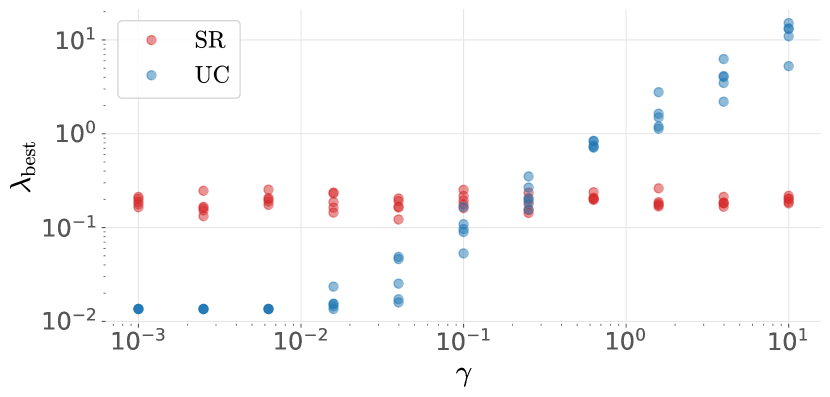
(a) $\lambda_{\text{best}}^{\text{SR}}$ and $\lambda_{\text{best}}^{\text{UC}}$ vs. noise scale $\gamma$, $5$ realizations each; $(m,n,s)=(50,100,5)$.

(b) Lipschitz behavior for each program; $L_{\text{SR}}$ as in Eq. 17, $L_{\text{UC}}$ as in Eq. 20. $V$ as in Corollary 5.7 gives $L_{\text{UC}}\approx L_{\text{SR}}|1-V|$.

Figure 2: Comparison between SR-LASSO (SR) and (unconstrained) LASSO (UC): recovery of an unknown sparse signal $x^{\sharp}\in\mathbb{R}^{n}$ from noisy underdetermined linear measurements (cf. Eq. 21). For $\lambda>0$, denote by $\bar{x}_{\text{SR}}(\lambda)$, $\bar{x}_{\text{UC}}(\lambda)\in\mathbb{R}^{n}$ respective solutions to SR-LASSO and LASSO. The optimal parameter values $\lambda_{\text{best}}^{\text{SR}},\lambda_{\text{best}}^{\text{UC}}>0$ for each program minimize the $\ell_{2}$ approximation error between the solution and $x^{\sharp}$. See §​ 6 for further details and discussion.

Our final contribution, in §​ 7, is a numerical exploration of SR-LASSO solution uniqueness and sensitivity, as well as an empirical verification of the tightness of our Lipschitz bounds in §​ 5 using synthetic experiments. In particular, Figs. 4 and 5 demonstrate a wide neighborhood in which the sufficient condition for uniqueness is empirically satisfied. Moreover, Fig. 6 supports the notion that our theoretical bounds on the Lipschitz constant for SR-LASSO are relatively tight (at least in the regime considered in the experiment).

1.3 Related work

The well-posedness study presented in this paper is inspired by the one for the LASSO problem in Zhang et al. [49], Gilbert [27] and Tibshirani [45], as well as the one for nuclear norm minimization by Hoheisel and Paquette [29]. The stability analysis executed here is similar to a study on the LASSO problem carried out by the authors of this paper [14]. Stability analysis for linear least-squares problems (i.e., quadratic fidelity term) with general, partially smooth regularizers can be found in the body of work by Vaiter et al., e.g., [46, 47]. This embeds in the more general and more recent studies (which do not cover the SR-LASSO) by Bolte et al. [18, 19]. A sensitivity analysis of the proximal operator using tools similar to our study can be found in Friedlander et al. [26]. Tuning parameter sensitivity has previously been examined for other LASSO formulations [15] and for proximal denoising [16].

Further studies that tackle the SR-LASSO explicitly, albeit not from a variational-analytic perspective, were discussed in §​ 1.1. They include contributions in the fields of statistics [10, 11, 20, 36, 41, 43, 48], sparse recovery, compressed sensing [1, 4, 3, 25, 31, 35], and deep learning [2, 5, 21].

1.4 Notation

In what follows, the Euclidean norm is denoted by $\|\cdot\|$, the $\ell_{1}$-norm (on $\mathbb{R}^{n}$) is given by $\|x\|_{1}:=\sum_{i=1}^{n}|x_{i}|$, while the $\ell_{\infty}$-norm (or maximum norm) is given by $\|x\|_{\infty}:=\max_{i=1,\dots,n}|x_{i}|$. The corresponding unit balls have the respective subscripts, i.e., $\mathbb{B}$, $\mathbb{B}_{1}$ and $\mathbb{B}_{\infty}$. The support of a vector $x\in\mathbb{R}^{n}$ is given by $\mathrm{supp}(x):=\left\{i\in\{1,\dots,n\}\,\left|\;x_{i}\neq 0\right.\right\}$. The first $n$ positive integers are denoted $[n]:=\{1,2,\ldots,n\}$. Define the projection operator onto a closed, convex set $C\subseteq\mathbb{R}^{n}$ by $\operatorname{P}_{C}(x):=\mathop{{\rm argmin}}_{z\in\mathbb{R}^{n}}\|z-x\|$. Write the orthogonal complement of a subspace $V\subseteq\mathbb{R}^{m}$ as $V^{\perp}$. The identity matrix is denoted by $\operatorname{\mathbb{I}}$. The spectral norm of a matrix $X\in\mathbb{R}^{m\times n}$ is denoted by $\|X\|$. For a set $K\subseteq[n]$, $X_{M}\in\mathbb{R}^{m\times|K|}$ is the matrix whose columns are the columns $X_{i}$ of $X$ for $i\in K$. For $x\in\mathbb{R}^{n}$, we let $L_{K}(x)\in\mathbb{R}^{n}$ be the vector whose elements are $x_{i}$ if $i\in K$ and $0$ otherwise.

2 Preliminaries

We start with some basic results from matrix analysis. Denote the (Moore-Penrose) pseudoinverse of $X$ by $X^{\dagger}$. For a symmetric matrix $S\in\mathbb{R}^{d\times d}$, let $\lambda_{\max}(S)$ be its maximum eigenvalue. For a matrix $X\in\mathbb{R}^{m\times s}$, let $\sigma_{\min}(X)$ be its smallest nonzero singular value, and let $\sigma_{\max}(X)$ be its maximum singular value. Recall that

$$\sigma_{\max}(X)=\|X\|=\sqrt{\lambda_{\max}(X^{T}X)}=\max_{v\in\mathbb{B}}v^{T}Xv.$$

We commence with a result that is ubiquitous in our study and is, in essence, the famous Sherman-Morrison-Woodbury formula [30, (0.7.4.1)].

Lemma 2.1 (Sherman-Morrison-Woodbury).

Let $M\in\mathbb{R}^{m\times s}$ such that $\mathrm{rank}\,M=s$, and let $v\in\mathbb{R}^{m}$ with $\|v\|=1$. For the matrix $W:=M^{\top}(\operatorname{\mathbb{I}}-vv^{\top})M$ the following hold:

• $W$ is invertible (in fact, symmetric positive definite) if (and only if) $v\notin\mathrm{rge}\,M$ with

  $$W^{-1}=(M^{\top}M)^{-1}+\frac{M^{\dagger}v(M^{\dagger}v)^{\top}}{1-v^{\top}MM^{\dagger}v}.$$

• In the invertible case, we have

  $$\lambda_{\max}(W^{-1})\leq\frac{1}{\sigma_{\min}(M)^{2}}+\frac{\|M^{\dagger}v\|^{2}}{1-v^{\top}MM^{\dagger}v}<\frac{1}{\sigma_{\min}(M)^{2}}+\frac{1}{1-v^{\top}MM^{\dagger}v}.$$

Proof 2.2.

(a) First, observe that with the invertible matrix $A:=M^{\top}M$, $x:=-M^{\top}v$, and $y:=-x$, we have

$$1+x^{\top}A^{-1}y=0 \iff 1=v^{\top}M(M^{\top}M)^{-1}M^{\top}v=v^{\top}MM^{\dagger}v=\|MM^{\dagger}v\|^{2}$$

$$\iff \|MM^{\dagger}v\|=\|v\|$$

$$\iff v\in\mathrm{rge}\,M.$$

The last equivalence follows from the fact that $MM^{\dagger}$ is the projection onto $\mathrm{rge}\,M$ and the Cauchy-Schwarz inequality. Hence, by the Sherman-Morrison-Woodbury formula [30, (0.7.4.1)] with $A,x,y$ as above, and assuming that $v\notin\mathrm{rge}\,M$, we have

$$W^{-1}=(M^{\top}M)^{-1}+\frac{(M^{\top}M)^{-1}M^{\top}vv^{\top}M(M^{\top}M)^{-1}}{1-v^{\top}M(M^{\top}M)^{-1}M^{\top}v}=(M^{\top}M)^{-1}+\frac{M^{\dagger}v(M^{\dagger}v)^{\top}}{1-v^{\top}MM^{\dagger}v}.$$

(b) By Weyl’s theorem [30, Theorem 4.3.1], it follows from (a) that

$$\lambda_{\max}(W^{-1}) \leq \lambda_{\max}((M^{\top}M)^{-1})+\lambda_{\max}\left(\frac{M^{\dagger}v(M^{\dagger}v)^{\top}}{1-v^{\top}MM^{\dagger}v}\right)$$

$$= \frac{1}{\sigma_{\min}(M)^{2}}+\frac{\|M^{\dagger}v\|^{2}}{1-\|MM^{\dagger}v\|^{2}}.$$

a

We record an immediate consequence.

Corollary 2.3.

Let $M\in\mathbb{R}^{m\times s}$ and let $v\in\mathbb{R}^{s}$ with $\|v\|=1$. Then the following are equivalent:

• $\ker M=\{0\}$ and $v\notin\mathrm{rge}\,M$;

• $\ker M^{\top}(\operatorname{\mathbb{I}}-vv^{\top})M=\{0\}$;

• $\ker(I-vv^{\top})M=\{0\}$.

Proof 2.4.

a

‘$(i)\Rightarrow(ii)$’: This follows immediately from Lemma 2.1(a).

‘$(ii)\Rightarrow(iii)$’: This is obvious.

‘$(iii)\Rightarrow(i)$’: Assume (i) were false. Then $\ker M$ is nontrivial, in which case so is $\ker(\operatorname{\mathbb{I}}-vv^{\top})M$, or $v\in\mathrm{rge}\,M$. The latter, however, implies that there exists $y\in\mathbb{R}^{s}\setminus\{0\}$ such that $(\operatorname{\mathbb{I}}-vv^{\top})My=(\operatorname{\mathbb{I}}-vv^{\top})v=0,$ hence, also in this case, $\ker(\operatorname{\mathbb{I}}-vv^{\top})M$ is nontrivial.

2.1 Tools from variational analysis

We provide in this section the necessary tools from variational analysis, and we follow here the notational conventions of Rockafellar and Wets [38], but the reader can find the objects defined here also in the books by Mordukhovich [32, 33] or Dontchev and Rockafellar [24].

Let $S:\mathbb{E}_{1}\rightrightarrows\mathbb{E}_{2}$ be a set-valued map. The domain and graph of $S$, respectively, are $\mathrm{dom}\,S:=\left\{x\in\mathbb{E}_{1}\,\left|\;S(x)\neq\emptyset\right.\right\}$ and $\mathrm{gph}\,S:=\left\{(x,y)\in\mathbb{E}_{1}\times\mathbb{E}_{2}\,\left|\;y\in S(x)\right.\right\}$. The outer limit of $S$ at $\bar{x}\in\mathbb{E}_{1}$ is

$$\mathop{{\rm Lim}\,{\rm sup}}_{x\to\bar{x}}S(x):=\left\{y\in\mathbb{E}_{2}\,\left|\;\exists\{x_{k}\}\to\bar{x},\{y_{k}\in S(x_{k})\}\to y\right.\right\}.$$

Now let $A\subseteq\mathbb{E}$. The tangent cone of $A$ at $\bar{x}\in A$ is $T_{A}(\bar{x}):=\mathop{{\rm Lim}\,{\rm sup}}_{t\downarrow 0}\frac{A-\bar{x}}{t}.$ The regular normal cone of $A$ at $\bar{x}\in A$ is the polar of the tangent cone, i.e.,

$$\hat{N}_{A}(\bar{x}):=T_{A}(\bar{x})^{\circ}=\left\{v\in\mathbb{E}\,\left|\;\left\langle v,\,y\right\rangle\leq 0\;\;\forall y\in T_{A}(\bar{x})\right.\right\}.$$

The limiting normal cone of $A$ at $\bar{x}\in A$ is $N_{A}(\bar{x}):=\mathop{{\rm Lim}\,{\rm sup}}_{x\to\bar{x}}\hat{N}_{A}(x).$ The coderivative of $S$ at $(\bar{x},\bar{y})\in\mathrm{gph}\,S$ is the map $D^{*}S(\bar{x}\mid\bar{y}):\mathbb{E}_{2}\rightrightarrows\mathbb{E}_{1}$ defined via

(3) $$v\in D^{*}S(\bar{x}\mid\bar{y})(y)\quad\Longleftrightarrow\quad(v,-y)\in N_{\mathrm{gph}\,S}(\bar{x},\bar{y}).$$

The graphical derivative of $S$ at $(\bar{x},\bar{y})$ is the map $DS(\bar{x}\mid\bar{y}):\mathbb{E}_{1}\rightrightarrows\mathbb{E}_{2}$ given by

(4) $$v\in DS(\bar{x}\mid\bar{y})(u)\quad\Longleftrightarrow\quad(u,v)\in T_{\mathrm{gph}\,S}(\bar{x},\bar{y}).$$

The strict graphical derivative of $S$ at $(\bar{x},\bar{y})$ is $D_{*}S(\bar{x}\mid\bar{y}):\mathbb{E}_{1}\rightrightarrows\mathbb{E}_{2}$ given by

$$D_{*}S(\bar{x}\mid\bar{y})(w)=\left\{z\in\mathbb{E}_{1}\,\left|\;\exists\left\{\begin{array}[]{l}\vspace{0.1cm}\{t_{k}\}\downarrow 0,\,\{w_{k}\}\to w,\\ \{z_{k}\}\to z,\\ \{(x_{k},y_{k})\in\mathrm{gph}\,S\}\to(\bar{x},\bar{y})\end{array}\right\}:z_{k}\in\frac{S(x_{k}+t_{k}w_{k})-y_{k}}{t_{k}}\right.\right\}.$$

We adopt the convention to set $D^{*}S(\bar{x}):=D^{*}S(\bar{x}\mid\bar{y})$ if $S(\bar{x})$ is a singleton, and proceed analogously for the graphical derivatives. We point out that if $S$ is single-valued and continuously differentiable at $\bar{x}$, then $DS(\bar{x})=D_{*}S(\bar{x})$ coincides with its derivative at $\bar{x}$. Moreover, in this case $D^{*}S(\bar{x})=DS(\bar{x})^{*}$. Therefore, there is, in this case, no ambiguity in notation. More generally, we will employ the following sum rule for the derivatives introduced above frequently in our study.

Lemma 2.5 ([38, Exercise 10.43 (b)]).

Let $S=f+F$ for $f:\mathbb{E}_{1}\to\mathbb{E}_{2}$, $F:\mathbb{E}_{1}\rightrightarrows\mathbb{E}_{2}$, and $(\bar{x},\bar{u})\in\mathrm{gph}\,S$. Assume that $f$ is continuously differentiable at $\bar{x}$. Then:

• $DS(\bar{x}|\bar{u})(w)=Df(\bar{x})w+DF(\bar{x}|\bar{u}-f(\bar{x}))(w),\quad\forall w\in\mathbb{E}_{1}$;

• $D_{*}S(\bar{x}|\bar{u})(w)=Df(\bar{x})w+D_{*}F(\bar{x}|\bar{u}-f(\bar{x}))(w),\quad\forall w\in\mathbb{E}_{1}$;

• $D^{*}S(\bar{x}|\bar{u})(y)=Df(\bar{x})^{*}y+D^{*}F(\bar{x}|\bar{u}-f(\bar{x}))(y),\quad\forall y\in\mathbb{E}_{2}$.

2.2 Convex analysis tools

We first present some fundamental concepts associated with convex sets [37]. For a convex set $C\subseteq\mathbb{R}^{n}$ and $\bar{x}\in C$ we define:

• the affine hull of $C$, i.e., is the smallest affine set that contains $C$, by $\mathrm{aff}\,C$;

• the subspace parallel to $C$ by $\mathrm{par}\,C:=\mathrm{span}\,(C-\bar{x})=\mathrm{aff}\,C-\bar{x};$

• its relative interior by $\mathrm{ri}\,C:=\left\{x\in C\,\left|\;\exists\varepsilon>0:\;B_{\varepsilon}(x)\cap\mathrm{aff}\,C\subseteq C\right.\right\}.$

We note that $\operatorname{int}C\neq\emptyset$ if and only if $\mathrm{par}\,C=\mathbb{R}^{n}$, in which case $\mathrm{ri}\,C=\operatorname{int}C$. We call a function $f:\mathbb{R}^{n}\to\mathbb{R}\cup\{+\infty\}$ proper if $\mathrm{dom}\,f:=\left\{x\in\mathbb{R}^{n}\,\left|\;f(x)<+\infty\right.\right\}$ is nonempty. It is called convex if its epigraph $\mathrm{epi}\,f:=\left\{(x,\alpha)\in\mathbb{R}^{n}\times\mathbb{R}\,\left|\;f(x)\leq\alpha\right.\right\}$ is a convex set. As a first, yet central, example of an extended real-valued function, we consider the indicator (function) $\delta_{C}:\mathbb{R}^{n}\to\mathbb{R}\cup\{+\infty\}$ of $C\subseteq\mathbb{R}$ given by

$$\delta_{C}(x)=\begin{cases}0&x\in C\\ +\infty&\text{else},\end{cases}$$

which is proper and convex if and only if $C$ is nonempty and convex. The (convex) subdifferential of $f:\mathbb{R}^{n}\to\mathbb{R}\cup\{+\infty\}$ at $\bar{x}\in\mathrm{dom}\,f$ is given by

$$\partial f(\bar{x})=\left\{v\in\mathbb{R}^{n}\,\left|\;f(\bar{x})+\left\langle v,\,x-\bar{x}\right\rangle\leq f(x)\;\forall x\in\mathrm{dom}\,f\right.\right\}.$$

For instance, the subdifferential of the indicator function of a convex set $C\subseteq\mathbb{R}^{n}$ at $\bar{x}\in C$ is the normal cone of $C$ at $\bar{x}$, i.e.,

$$\partial\delta_{C}(\bar{x})=\left\{v\in\mathbb{R}^{n}\,\left|\;\left\langle v,\,x-\bar{x}\right\rangle\leq 0\quad\forall x\in C\right.\right\}=N_{C}(\bar{x}).$$

The two most important examples to our study are the Euclidean norm $\|\cdot\|$ whose subdifferential is given by

(6) $$\partial\|\cdot\|(z)=\begin{cases}\left\{\frac{z}{\|z\|}\right\}&z\neq 0\\ \mathbb{B}&z=0,\end{cases}$$

and the $\ell_{1}$-norm whose subdifferential is presented in the next result.

Lemma 2.6 (Subdifferential of $\ell_{1}$-norm).

Let $z\in\mathbb{R}^{n}$ and set $I:=\mathrm{supp}(z):$

• $\partial\|\cdot\|_{1}(z)=\bigtimes_{i=1}^{n}\left.\begin{cases}\mathrm{sgn}(z_{i}),&z_{i}\neq 0,\\ [-1,1],&z_{i}=0\end{cases}\right\}$;

• $\mathrm{ri}\,\partial\|\cdot\|_{1}(z)=\bigtimes_{i=1}^{n}\left.\begin{cases}\mathrm{sgn}(z_{i}),&z_{i}\neq 0,\\ (-1,1),&z_{i}=0\end{cases}\right\}$;

• $\mathrm{par}\,\partial\|\cdot\|_{1}(z)=\left\{v\in\mathbb{R}^{n}\,\left|\;v_{I}=0\right.\right\}$.

The (Fenchel) conjugate of $f:\mathbb{R}^{n}\to\mathbb{R}\cup\{+\infty\}$ is the function $f^{*}:\mathbb{R}^{n}\to\mathbb{R}\cup\{+\infty\}$,

$$f^{*}(y):=\sup_{x\in\mathrm{dom}\,f}\{\left\langle y,\,x\right\rangle-f(x)\}.$$

If $f$ is proper and convex, then so is $f^{*}$ (which is always lower semicontinuous). Of special interest is the conjugacy relation between indicator and support functions. For any set $C\subseteq\mathbb{R}^{n}$, its support function is $\sigma_{C}(y):=\sup_{x\in C}\left\langle x,\,y\right\rangle=\delta^{*}_{C}(y)$. We have $\sigma_{C}^{*}(y)=\delta_{C}(x)$ if (and only if) $C$ is nonempty, closed and convex. This is relevant to our study as every norm is the support function of a symmetric, convex, compact set $C$ with $0\in\operatorname{int}C$. In particular, $\|\cdot\|_{p}=\sigma_{\mathbb{B}_{q}}$ for all $1\leq p,q\leq\infty$ and $\frac{1}{p}+\frac{1}{q}=1$, eg see [38, 11(12)]. Consequently, we have

(7) $$\|\cdot\|^{*}=\delta_{\mathbb{B}}\and\|\cdot\|_{1}^{*}=\delta_{\mathbb{B}_{\infty}}.$$

3 Uniqueness of solutions and regularity conditions for SR-LASSO

This section establishes a sufficient condition for SR-LASSO solution uniqueness, then introduces two stronger point-based regularity conditions and their relationship.

3.1 Uniqueness of solutions

In this section, we provide conditions that guarantee a given solution of SR-LASSO is unique. The key observation is that the normalized residual is, in essence, an invariant for a given problem instance. This fact can be seen through (Fenchel-Rockafellar) duality (e.g., see [38, Chapter 11]), which we establish for the SR-LASSO Eq. 1 here.

Proposition 3.1 (Fenchel-Rockafellar duality scheme for Eq. 1).

We have:

• The (Fenchel-Rockafellar) dual problem to Eq. 1 is

  (8) $$\max_{y\in\mathbb{R}^{m}}\;\left\langle b,\,y\right\rangle\ \mbox{s.t.}\ A^{\top}y\in\lambda\mathbb{B}_{\infty},\quad y\in\mathbb{B}.$$

• For $(\bar{x},\bar{y})$ the following are equivalent:

  • $\bar{x}$ solves Eq. 1, $\bar{y}$ solves Eq. 8.

  • $\|A\bar{x}-b\|_{2}+\lambda\|\bar{x}\|_{1}=\left\langle b,\,\bar{y}\right\rangle$, and $\bar{y}$ is feasible for Eq. 8.

  • $A^{\top}\bar{y}\in\lambda\partial\|\cdot\|_{1}(\bar{x})$,  $-\bar{y}\in\partial\|(\cdot)-b\|_{2}(A\bar{x})$.

  • $\bar{x}\in N_{\lambda\mathbb{B}_{\infty}}(A^{\top}\bar{y}),$  $b-A\bar{x}\in N_{\mathbb{B}}(\bar{y})$.

Proof 3.2.

Apply [38, Example 11.41] in combination with Lemma 2.6, Eq. 6 and Eq. 7, and realize that strong duality holds (as the the primal functions are finite-valued), i.e., primal and dual optimal value are identical, which explains the equivalence of (i) and (ii).

We now present the advertised invariance of the normalized residual.

Corollary 3.3.

If there exists a solution $\hat{x}$ of Eq. 1 with $A\hat{x}-b\neq 0$, then:

• The dual problem Eq. 8 has a unique solution $\bar{y}$ with $\|\bar{y}\|=1$.

• Every solution $\bar{x}$ of Eq. 1 satisfies $b-A\bar{x}=\|A\bar{x}-b\|\bar{y}$.

Proof 3.4.

(a) Observe that every dual solution $\bar{y}$, by Proposition 3.1(b), must satisfy

$$-\bar{y}\in\partial\|\cdot\|(A\hat{x}-b)=\left\{\frac{A\hat{x}-b}{\|A\hat{x}-b\|}\right\}.$$

(b) Let $\bar{y}$ be the unique dual solution. Pick any $\bar{x}$ that solves Eq. 1 such that $A\bar{x}-b\neq 0$. Then, by Proposition 3.1 (b), it follows that $\bar{y}=\frac{b-A\bar{x}}{\|A\bar{x}-b\|}$.

We record a simple linear-algebraic fact.

Lemma 3.5.

Let $0\in A\subseteq\mathbb{R}^{n}$ and let $U\subseteq\mathbb{R}^{n}$ be a subspace. Then $\mathrm{span}\,(U+A)=U+\mathrm{span}\,A$.

Proof 3.6.

First, observe that $U+A\subseteq U+\mathrm{span}\,A$, hence $\mathrm{span}\,(U+A)\subseteq U+\mathrm{span}\,A$.

In turn, observe that $U\subseteq U+A\subseteq\mathrm{span}\,(U+A)$ and $\mathrm{span}\,A\subseteq\mathrm{span}\,(U+A)$ (since both $U$ and $A$ contain $0$). Consequently, we have

$$U+\mathrm{span}\,A=\mathrm{span}\,(U\cup\mathrm{span}\,A)\subseteq\mathrm{span}\,(U+A).$$

The main result on uniqueness relies on the following regularity condition that we impose at a solution $\bar{x}$ of Eq. 1.

Assumption 1 (Weak).

For a solution $\bar{x}$ of Eq. 1 with $I:=\mathrm{supp}(\bar{x})$ we have:

• $\ker A_{I}=\{0\}\and b\notin\mathrm{rge}\,A_{I}$;

• $\exists z\in\left\{\frac{b-A\bar{x}}{\|A\bar{x}-b\|}\right\}^{\perp}\cap\ker A_{I}^{\top}:\left\|A_{I^{C}}^{\top}\left(\frac{b-A\bar{x}}{\|A\bar{x}-b\|}+z\right)\right\|_{\infty}<\lambda$.

We are now in a position to present the advertised uniqueness result.

Theorem 3.7 (Uniqueness of solutions).

Under 1, $\bar{x}$ is the unique solution of Eq. 1.

Proof 3.8.

Let $\bar{y}:=\frac{b-A\bar{x}}{\|A\bar{x}-b\|}$ denote the unique dual solution and consider the auxiliary problem with $\mathcal{S}:=N_{\mathbb{B}}(\bar{y})=\mathbb{R}_{+}\{\bar{y}\}$:

(9) $$\min_{x\in\mathbb{R}^{n}}\psi(x):=\lambda\|x\|_{1}-\left\langle A^{\top}\bar{y},\,x\right\rangle+\delta_{\mathcal{S}}(b-Ax).$$

The optimality conditions for Eq. 9 read

$$0\in\partial\psi(x)=\lambda\partial\|\cdot\|_{1}(x)-A^{\top}\bar{y}-A^{\top}N_{\mathcal{S}}(b-Ax),\quad b-Ax\in\mathcal{S}.$$

Using Corollary 3.3(b) and the fact that $0\in N_{\mathcal{S}}(b-Ax)$, we see that every solution of Eq. 1 solves Eq. 9. Now, $\bar{x}$ is the unique solution of Eq. 9 if (and only if) $0\in\operatorname{int}\partial\psi(\bar{x})$ [27, Lemma 3.2]. Since $A\bar{x}-b\neq 0$, we find that $N_{\mathcal{S}}(b-A\bar{x})=\{\bar{y}\}^{\perp}=\mathrm{rge}\,P$, where $P:=\operatorname{\mathbb{I}}-\bar{y}\bar{y}^{\top}$ is the orthogonal projection onto $\{\bar{y}\}^{\perp}$. We now observe that $0\in\operatorname{int}\partial\psi(\bar{x})$ if and only if the following two conditions hold:

$$\mathrm{span}\,\partial\psi(\bar{x})=\mathbb{R}^{n}\and 0\in\mathrm{ri}\,\partial\psi(\bar{x}).$$

Since our assumptions imply that $N_{\mathcal{S}}(b-A\bar{x})=\mathrm{rge}\,P$, we find that

$$\mathrm{span}\,\partial\psi(\bar{x})=\mathbb{R}^{n} \iff \mathrm{par}\,\partial\|\cdot\|_{1}(\bar{x})+\mathrm{rge}\,(A^{\top}P)=\mathbb{R}^{n}$$

$$\iff \left(\mathrm{par}\,\partial\|\cdot\|_{1}(\bar{x})\right)^{\perp}\cap\ker(PA)=\{0\}$$

$$\iff \ker(PA_{I})=\{0\}$$

$$\iff \ker A_{I}=\{0\}\and b\notin\mathrm{rge}\,A_{I}.$$

Here the first identity uses Lemma 3.5 and the fact that $A^{\top}\bar{y}\in\lambda\partial\|\cdot\|_{1}(\bar{x})$. The second one follows by taking orthogonal complements on both sides. The penultimate equivalence uses Lemma 2.6 (b), and the last equivalence uses Corollary 2.3.

In addition, we observe that

$$0\in\mathrm{ri}\,\partial\psi(\bar{x}) \iff \exists z\in\{\bar{y}\}^{\perp}:A_{i}^{\top}\bar{y}\in\lambda\mathrm{ri}\,\partial|\cdot|(\bar{x}_{i})-A_{i}^{\top}z,$$

which can be seen to be equivalent to (ii) by Lemma 2.6 (b).

Remark 3.9.

Note that for $I=\emptyset$ (i.e., $\bar{x}=0$), condition (i) is vacuously satisfied, so the sufficient conditions collapse to

(10) $$\exists z\in\{b\}^{\perp}:\|A_{I^{C}}^{\top}(b/\|b\|+z)\|_{\infty}<\lambda.$$

The former corresponds to the fact that for $\bar{x}=0$, we have $\mathrm{par}\,\partial\psi(\bar{x})=\mathbb{R}^{n}$. $\diamond$

3.2 Stronger regularity conditions

We now introduce two additional regularity conditions, both of which (will be seen to) imply 1, and hence also guarantee well-posedness of the SR-LASSO. As we will see in §​ 4 and §​ 5, respectively, these conditions in fact yield stability of the solution function.

3.2.1 Intermediate condition

We start with what we call the intermediate condition. This condition is based on the notion of the (SR-LASSO) equicorrelation set, which is an analog to the one in the LASSO setting [45].

Assumption 2 (Intermediate).

For a minimizer $\bar{x}$ of Eq. 1, we have $A\bar{x}\neq b$ and for

$$J:=\left\{i\in[n]\,\left|\;\left|A_{i}^{T}\frac{b-A\bar{x}}{\|A\bar{x}-b\|}\right|=\lambda\right.\right\},$$

we have $\ker A_{J}=\{0\}$ and $b\notin\mathrm{rge}\,A_{J}$.

Observe that if $\bar{x}$ is minimizer of Eq. 1 with $A\bar{x}\neq b$, then we have $I:=\mathrm{supp}(\bar{x})\subseteq J$ by first-order optimality conditions; a fact that is frequently used from here on.

We will now show that 2 implies 1 as advertised. To this end, we employ the following lemma, whose proof is deferred to Appendix A.

Lemma 3.10 (Shrinking property).

Let $B\in\mathbb{R}^{m\times\ell},C\in\mathbb{R}^{m\times s},\bar{y}\in\mathbb{R}^{m}$ and $\varepsilon>0$ such that $\mathrm{rank}\,[B\;C]=\ell+s$ and $\bar{y}\notin\mathrm{rge}\,[B\;C]$. Set $\mathcal{T}:=\{\bar{y}\}^{\perp}\cap\ker C^{\top}$ and

$$p^{*}:=\inf_{z\in\varepsilon\mathbb{B}\cap\mathcal{T}}\|B^{\top}(\bar{y}+z)\|_{\infty}.$$

Then, $p^{*}<\|B^{\top}\bar{y}\|_{\infty}$, and the infimum is attained.

We are now in a position to present the advertised implication.

Proposition 3.11.

2 implies 1.

Proof 3.12.

Let $\bar{x}$ solve Eq. 1, set $I:=\mathrm{supp}(\bar{x})$ and $s:=|I|$. Note that $b\notin\mathrm{rge}\,A_{J}$, thus, in particular, $b\notin\mathrm{rge}\,A_{I}$ and $A\bar{x}\neq b$, so $\bar{y}:=\frac{b-A\bar{x}}{\|A\bar{x}-b\|}$ is the unique dual solution (cf. Corollary 3.3). Thus, to establish the result, we show that

$$\exists\;z\in\{\bar{y}\}^{\perp}\cap\ker A_{I}^{T}:\;\|A_{I^{C}}^{\top}(\bar{y}+z)\|_{\infty}<\lambda.$$

Now, set $\mathcal{T}:=\{\bar{y}\}^{\perp}\cap\ker A_{I}^{\top}$. Since one already has $\|A_{J^{C}}^{\top}\bar{y}\|_{\infty}<\lambda$ by definition of $J$, choose any $\varepsilon>0$ satisfying

$$\sup_{z\in\varepsilon\mathbb{B}\cap\mathcal{T}}\|A_{J^{C}}^{\top}(\bar{y}+z)\|_{\infty}<\lambda,$$

and seek $z\in\varepsilon\mathbb{B}\cap\mathcal{T}$ satisfying $\|A_{J\setminus I}^{\top}(\bar{y}+z)\|_{\infty}<\lambda$. We select such a $z$ via Lemma 3.10 with $B:=A_{J\setminus I},C:=A_{I}$ and $\ell:=|J\setminus I|=|J|-s$. Thus, one has $\mathrm{rank}\,[A_{J\setminus I}\;A_{I}]=\mathrm{rank}\,A_{J}=|J|$, and $\bar{y}\notin\mathrm{rge}\,A_{J}=\mathrm{rge}\,[A_{J\setminus I}\;A_{I}]$. Therefore, the lemma yields $\bar{z}\in\varepsilon\mathbb{B}\cap\mathcal{T}$ satisfying $\|A_{J\setminus I}^{\top}(\bar{y}+\bar{z})\|_{\infty}<\|A_{J\setminus I}^{\top}\bar{y}\|_{\infty}=\lambda$. Consequently, there exists $\bar{z}\in\mathcal{T}$ satisfying $\|A_{I^{C}}^{\top}(\bar{y}+\bar{z})\|_{\infty}<\lambda$, completing the proof.

An immediate consequence of the above result and Theorem 3.7 is that the intermediate condition from 2 yields uniqueness of the solution in question. This is complemented by the following result, the proof of which is postponed to Appendix B. Under 2, it establishes uniqueness and gives an analytic expression for the unique solution, analogous to a result for unconstrained LASSO [45, Lemma 2].

Proposition 3.13 (Analytic solution formula).

Let $\bar{x}$ be a solution of Eq. 1 such that 2 holds at $\bar{x}$. Then $\bar{x}$ is the unique solution and

(11) $$\bar{x}=L_{J}\left(BA_{J}^{\top}(\operatorname{\mathbb{I}}-\bar{y}\bar{y}^{\top})b\right),\qquad B:=\left[A_{J}^{\top}(\operatorname{\mathbb{I}}-\bar{y}\bar{y}^{\top})A_{J}\right]^{-1}.$$

3.2.2 The strong condition

We present a third regularity condition to which we will refer as the ‘strong’ condition as it implies the intermediate condition from 2 (and thus the weak one) as we will see shortly.

Assumption 3 (Strong).

For a minimizer $\bar{x}$ of Eq. 1 with $I:=\mathrm{supp}(\bar{x})$ we have:

• $\ker A_{I}=\{0\}$ and $b\notin\mathrm{rge}\,A_{I}$;

• $\|A_{I^{C}}^{\top}(b-A\bar{x})\|_{\infty}<\lambda\|A\bar{x}-b\|$.

Remark 3.14 (On 3).

Note that part (ii) is automatically satisfied if $\|A_{I^{C}}^{\top}\|_{2\to\infty}<\lambda$, where $\|\cdot\|_{2\to\infty}$ denotes the induced matrix norm defined by $\|M\|_{2\to\infty}:=\sup_{\|z\|_{2}=1}\|Mz\|_{\infty}$. In particular, (ii) is implied by $\|A_{I^{C}}^{\top}\|<\lambda$ since $\|M\|_{2\to\infty}\leq\|M\|$ for any matrix $M$. $\diamond$

We now address the advertised (and trivial) implication.

Proposition 3.15.

3 implies 2.

Proof 3.16.

If 3 holds at $\bar{x}$, then part (ii) yields that $I=J$, hence part (ii) implies that $A_{J}=A_{I}$ has full rank.

3.2.3 Overview of regularity conditions

From Proposition 3.11 and Proposition 3.15 it follows that:

3  $\Longrightarrow$  2 $\Longrightarrow$  1.

The reverse implications do not generally hold as the following examples show.

Example 3.17.

Consider the SR-LASSO Eq. 1 with

$$A=\begin{pmatrix}1&0&0\\ 0&1&1\end{pmatrix},\and b=\binom{1}{2}.$$

For $\lambda=\frac{2}{\sqrt{5}}$, we find that $\bar{x}=0$ is a solution (with $I=\emptyset$) as

$$A^{T}\frac{b-A\bar{x}}{\|A\bar{x}-b\|}=A^{T}\frac{b}{\|b\|}=\begin{pmatrix}\lambda/2\\ \lambda\\ \lambda\end{pmatrix}\in\lambda\partial\|\cdot\|_{1}(\bar{x}).$$

We also see that $J=\{2,3\}$, so $A_{J}=\begin{pmatrix}0&0\\ 1&1\end{pmatrix}$. Consequently, 2 is violated at $\bar{x}$. In turn, let $\bar{z}:=\frac{\lambda}{6}\binom{\hphantom{-}2}{-1}\in\{b\}^{\perp}$. Then, with $A_{I^{C}}=A$, we find

$$\left\|A_{I^{C}}^{T}\left(\frac{b}{\|b\|}+\bar{z}\right)\right\|_{\infty}=\left\|\begin{pmatrix}\lambda/2\\ \lambda\\ \lambda\end{pmatrix}+\begin{pmatrix}\lambda/3\\ -\lambda/6\\ -\lambda/6\end{pmatrix}\right\|_{\infty}<\lambda.$$

Therefore, in view of Eq. 10, 1 holds at $\bar{x}$. $\diamond$

Example 3.18.

Consider the SR-LASSO Eq. 1 with

$$A:=\begin{pmatrix}1&0&2\\ 0&2&-2\end{pmatrix}\and b:=\begin{pmatrix}1\\ 1\end{pmatrix}.$$

For $\lambda=\sqrt{2}$, we find that $\bar{x}=0$ is a solution (with $I=\emptyset$) as

$$A^{T}\frac{b-A\bar{x}}{\|A\bar{x}-b\|}=A^{T}\frac{b}{\|b\|}=\begin{pmatrix}\frac{1}{\lambda}\\ \lambda\\ 0\end{pmatrix}\in\lambda\partial\|\cdot\|_{1}(\bar{x}).$$

In particular, $J=\{2\}$, thus $A_{J}=\binom{0}{2}$, hence 2 is satisfied. In turn, 3 is violated as $I\subsetneq J$. $\diamond$

4 Lipschitz stability under the intermediate condition

In this section, we show that the intermediate condition 2 yields directional differentiability and local Lipschitz continuity of the solution function of the SR-LASSO Eq. 1 at the point in question, and we provide explicit Lipschitz bounds. The key result is that, under 2, the subdifferential map of the objective function of the SR-LASSO is strongly metrically regular [24, 38] at the point in question, i.e., it is invertible with locally Lipschitz inverse there. To this end, given a positively homogenous map $H:\mathbb{R}^{n}\rightrightarrows\mathbb{R}^{m}$, its outer norm given by

$$|H|^{+}:=\sup_{\|x\|\leq 1}\sup_{y\in H(x)}\|y\|.$$

Proposition 4.1.

Let $A\in\mathbb{R}^{m\times n}$, $b\in\mathbb{R}^{m}$ and let $\bar{x}\in\mathbb{R}^{n}$ be a solution of Eq. 1 such that $b\neq A\bar{x}$. Define $T:\mathbb{R}^{n}\rightrightarrows\mathbb{R}^{n}$ by $T(x):=\frac{1}{\lambda}\partial\left(\|A(\cdot)-b\|\right)(x)+\partial\|\cdot\|_{1}(x)$. Under 2, $\left|D^{*}T(\bar{x}\mid 0)^{-1}\right|^{+}<\infty$. Moreover, $T$ is strongly metrically regular at $(\bar{x},0)$.

Proof 4.2.

Define $\bar{r}:=b-A\bar{x}$ and $\bar{y}:=\bar{r}/\|\bar{r}\|$. Let $G:=\nabla\|A(\cdot)-b\|$ and observe that $G$ has the form $G=\phi(A,b,1,\cdot)$ for $\phi$ as defined in Lemma C.1. By Lemma 2.5(c), Lemma C.1(d) and the symmetry of $DG(\bar{x})$, one has

$$D^{*}T(\bar{x}\mid 0)(y) =\frac{1}{\lambda}DG(\bar{x})y+D^{*}\left(\partial\|\cdot\|_{1}\right)\left(\bar{x}\mid\frac{1}{\lambda}A^{\top}\bar{y}\right)(y)$$

$$=\frac{1}{\lambda\|\bar{r}\|}A^{\top}\left(\operatorname{\mathbb{I}}-\bar{y}\bar{y}^{\top}\right)Ay+D^{*}\left(\partial\|\cdot\|_{1}\right)\left(\bar{x}\mid\frac{1}{\lambda}A^{\top}\bar{y}\right)(y).$$

Thus, we have

$$y\in D^{*}T(\bar{x}\mid 0)^{-1}(z)$$

$$\iff z\in D^{*}T\left(\bar{x}\mid 0\right)(y)$$

$$\iff z-\frac{1}{\lambda\|\bar{r}\|}A^{\top}\left(\operatorname{\mathbb{I}}-\bar{y}\bar{y}^{\top}\right)Ay\in D^{*}\left(\partial\|\cdot\|_{1}\right)\left(\bar{x}\mid\frac{1}{\lambda}A^{\top}\bar{y}\right)(y)$$

$$\iff \left(z-\frac{1}{\lambda\|\bar{r}\|}A^{\top}\left(\operatorname{\mathbb{I}}-\bar{y}\bar{y}^{\top}\right)Ay,-y\right)\in N_{\mathrm{gph}\,\partial\|\cdot\|_{1}}\left(\bar{x},\frac{1}{\lambda}A^{\top}\bar{y}\right)$$

$$\implies \begin{cases}\left(z_{i}-\frac{1}{\lambda\|\bar{r}\|}A_{i}^{\top}\left(\operatorname{\mathbb{I}}-\bar{y}\bar{y}^{\top}\right)Ay,-y_{i}\right)\in\mathbb{R}\times\{0\},&\forall i\in J^{C},\\ \left(z_{i}-\frac{1}{\lambda\|\bar{r}\|}A_{i}^{\top}\left(\operatorname{\mathbb{I}}-\bar{y}\bar{y}^{\top}\right)Ay,-y_{i}\right)\in\{0\}\times\mathbb{R},&\forall i\in I,\\ \left(z_{i}-\frac{1}{\lambda\|\bar{r}\|}A_{i}^{\top}\left(\operatorname{\mathbb{I}}-\bar{y}\bar{y}^{\top}\right)Ay,-y_{i}\right)\in\mathbb{R}_{-}\times\mathbb{R}_{+}\cup\mathbb{R}_{+}\times\mathbb{R}_{-},&\forall i\in J\setminus I.\end{cases}$$

The third equivalence holds by definition of the coderivative, and the final implication can be obtained, for instance, from [14, Lemma 4.9]. The first two conditions, for $J^{C}$ and $I$, respectively, yield $y_{J^{C}}=0$ and $\lambda\|\bar{r}\|z_{I}=A_{I}^{\top}\left(\operatorname{\mathbb{I}}-\bar{y}\bar{y}^{\top}\right)A_{J}y_{J}$. Notice that the third condition (using $y_{J^{C}}\equiv 0$) implies

$$y_{i}\left(z_{i}-\frac{1}{\lambda\|\bar{r}\|}A_{i}^{\top}\left(\operatorname{\mathbb{I}}-\bar{y}\bar{y}^{\top}\right)A_{J}y_{J}\right)\geq 0\qquad\forall i\in J\setminus I.$$

Combining this observation with the first two conditions yields

(12) $$y_{J}^{\top}z_{J}-\frac{1}{\lambda\|\bar{r}\|}y_{J}^{\top}A_{J}^{\top}(\operatorname{\mathbb{I}}-\bar{y}\bar{y}^{\top})A_{J}y_{J}\geq 0\quad\forall z\in D^{*}T\left(\bar{x}\mid 0\right)(y).$$

Therefore, we find that

$$\left|D^{*}T(\bar{x}\mid 0)^{-1}\right|^{+} =\sup_{(z,y)\in\mathbb{R}^{n}\times\mathbb{R}^{n}}\left\{\|y\|\mid\|z\|\leq 1,y\in D^{*}T(\bar{x}\mid 0)^{-1}(z)\right\}$$

$$\leq\sup_{(z,u)\in\mathbb{R}^{n}\times\mathbb{R}^{|J|}}\left\{\|u\|\,\left|\;\|z\|\leq 1,\;u^{\top}z_{J}\geq\frac{1}{\lambda\|\bar{r}\|}u^{\top}A_{J}^{\top}(\operatorname{\mathbb{I}}-\bar{y}\bar{y}^{\top})A_{J}u\right.\right\}$$

$$<+\infty.$$

Here the finiteness is due to the fact that the second supremum is attained by compactness of the constrained set which, in turn, relies on the positive definiteness of $A_{J}^{\top}(\operatorname{\mathbb{I}}-\bar{y}\bar{y}^{\top})A_{J}$ due to 2 and Lemma 2.1. Hence, by [24, Theorem 4C.2] it follows that $T$ is metrically regular at $(\bar{x},0)$. In addition, a subdifferential of a closed, proper convex function, $T$ is globally (maximally) monotone, so by [24, Theorem 3G.5], it follows that $T$ is strongly metrically regular at $(\bar{x},0)$.

We use the strong metric regularity result under 2 to bootstrap our way to directional differentiability and obtain a (local) Lipschitz modulus for the solution map that depends on $J$. For this, we need the following preparatory result.

Lemma 4.3.

Let $\bar{x}$ be the (unique) solution of Eq. 1 such that (given $(A,b,\lambda)$) 2 holds at $\bar{x}$. Suppose that $\bar{x}_{k}$ solves Eq. 1 given $(A_{k},b_{k},\lambda_{k})\to(A,b,\lambda)$ and assume $\bar{x}_{k}\to\bar{x}$. Then, 2 holds at $\bar{x}_{k}$ (for $(A_{k},b_{k},\lambda_{k})$).

Proof 4.4.

First, note that $A\bar{x}\neq b$. As $(A_{k},b_{k})\to(A,b)$ and $\bar{x}_{k}\to\bar{x}$, by continuity we find that $A_{k}\bar{x}_{k}\neq b_{k}$ for all $k$ sufficiently large. In particular, the equicorrelation set $J_{k}$ associated to $\bar{x}_{k}$ and $(A_{k},b_{k},\lambda_{k})$ is well-defined for such $k$, and by continuity, $J_{k}\subseteq J$ for all $k$ sufficiently large. Since $A_{J}$ has full rank, so does $A_{J_{k}}$ for all $k$ sufficiently large.

We are now in a position to state the main result of this section. Recall that we already know from Proposition 3.11 and Theorem 3.7 that the intermediate condition in 2 implies uniqueness of solutions at the point in question.

Theorem 4.5.

Let $(\bar{b},\bar{\lambda})\in\mathbb{R}^{m}\times\mathbb{R}_{++}$ and suppose that 2 holds at $\bar{x}:=S(\bar{b},\bar{\lambda})$, where $S$ is defined as in Eq. 2. Then:

1. $S$ is locally Lipschitz at $(\bar{b},\bar{\lambda})$ with (local) Lipschitz modulus

   $$L\leq\left[\frac{1}{\sigma_{\min}(A_{J})^{2}}+\frac{1}{1-\|A_{J}A_{J}^{\dagger}\bar{y}\|}\right]\cdot\left[\sigma_{\max}\left(A_{J}\right)+\left\|\frac{A_{J}^{\top}(A\bar{x}-\bar{b})}{\bar{\lambda}}\right\|\right].$$

2. $S$ is directionally differentiable at $(\bar{b},\bar{\lambda})$ and the directional derivative
   $S^{\prime}((\bar{b},\bar{\lambda});(\cdot,\cdot)):\mathbb{R}^{m}\times\mathbb{R}\to\mathbb{R}^{n}$ is locally Lipschitz. Moreover, for $(q,\alpha)\in\mathbb{R}^{m}\times\mathbb{R}$ there exists $K=K(q,\alpha)\subseteq J$ with $\mathrm{supp}(\bar{x})\subseteq K$ such that

   $$S^{\prime}((\bar{b},\bar{\lambda});(q,\alpha))=L_{K}\left(B\left(A_{K}^{\top}(\operatorname{\mathbb{I}}-\bar{y}\bar{y}^{\top})q+\frac{\alpha}{\bar{\lambda}}A_{K}^{\top}(AS(\bar{b},\bar{\lambda})-\bar{b})\right)\right),$$

   where $B:=\left(A_{K}^{\top}A_{K}\right)^{-1}+\dfrac{A_{K}^{\dagger}\bar{y}(A_{K}^{\dagger}\bar{y})^{\top}}{1-\bar{y}^{\top}A_{K}A_{K}^{\dagger}\bar{y}}$.

Proof 4.6.

We apply [14, Proposition 4.10] for $f:(\mathbb{R}^{m}\times\mathbb{R})\times\mathbb{R}^{n}\to\mathbb{R}^{n}$ with

$$f((b,\lambda),x)=\frac{1}{\lambda}A^{\top}\partial\|\cdot\|_{2}(Ax-b),\quad\forall b\in\mathbb{R}^{m},\;\forall\lambda>0,\;\forall x\in\mathbb{R}^{n},$$

and $F:\mathbb{R}^{n}\rightrightarrows\mathbb{R}^{n},\;F:=\partial\|\cdot\|_{1}$. Throughout, to simplify notation, we make the identification $f(b,\lambda,x):=f((b,\lambda),x)$ (and perform this unnesting elsewhere, where appropriate). Under 2, it holds that $A\bar{x}\neq\bar{b}$, hence, $f$ is continuously differentiable in a neighborhood of $(\bar{b},\bar{\lambda},\bar{x})$. Additionally, $f$ and $F$ are monotone, because the (sub)differential operator of a convex function is (maximally) monotone [38, Chapter 12]. We organize the proof into three steps.

Step 1. Local Lipschitz continuity of $S$

By construction, $(\bar{b},\bar{\lambda},\bar{x})\in\mathrm{gph}\,S$ with $0\in f(\bar{b},\bar{\lambda},\bar{x})+F(\bar{x})$. For $T(x):=f(\bar{b},\bar{\lambda},x)+F(x)$, as in Proposition 4.1, Lemma 2.5 yields

$$D^{*}T(\bar{x}\mid 0)=D_{x}f(\bar{b},\bar{\lambda},\bar{x})^{*}+D^{*}F(\bar{x}\mid-f(\bar{b},\bar{\lambda},\bar{x})).$$

Hence, Proposition 4.1 establishes finiteness of $\left|\left(D^{*}T(\bar{x}\mid 0)\right)^{-1}\right|^{+}$, giving local Lipschitz continuity of $S$ at $(\bar{b},\bar{\lambda})$ by [14, Proposition 4.10(b)] and showing the validity of the first claim in part (a).

Step 2. Directional differentiability of $S$ at $(\bar{b},\bar{\lambda})$

Observe that

$$S(b,\lambda)=\{x\in\mathbb{R}^{n}:0\in G(b,\lambda,x)\},\quad\text{with }G(b,\lambda,x):=f(b,\lambda,x)+F(x).$$

Moreover, $F$ is proto-differentiable at $(\bar{x},-f(\bar{b},\bar{\lambda},\bar{x}))$ by [26, Remark 1 and Lemma 4]. Hence, by [14, Proposition 4.10(c)], the graphical derivative $DS(\bar{b},\bar{\lambda})$ is (single-valued and) locally Lipschitz with

$$DS(\bar{b},\bar{\lambda})(q,\alpha)=\left\{w\in\mathbb{R}^{n}:0\in DG(\bar{b},\bar{\lambda},\bar{x}\mid 0)(q,\alpha,w)\right\},\qquad\forall(q,\alpha)\in\mathbb{R}^{m}\times\mathbb{R}.$$

Using the graphical derivative sum rule in Lemma 2.5(a) gives

$$DG(\bar{b},\bar{\lambda},\bar{x}\mid 0)(q,\alpha,w)=Df(\bar{b},\bar{\lambda},\bar{x})(q,\alpha,w)+DF(\bar{x}\mid-f(\bar{b},\bar{\lambda},\bar{x}))(w),$$

where $Df(\bar{b},\bar{\lambda},\bar{x}\mid 0)(q,\alpha,w)=D_{b}f(\bar{b},\bar{\lambda},\bar{x})q+D_{\lambda}f(\bar{b},\bar{\lambda},\bar{x})\alpha+D_{x}f(\bar{b},\bar{\lambda},\bar{x})w$. Letting $\bar{r}:=\bar{b}-A\bar{x}$ and $\bar{y}:=\bar{r}/\|\bar{r}\|$, we use Lemma C.1 to compute:

$$Df(\bar{b},\bar{\lambda},\bar{x})(q,\alpha,w) =-\frac{1}{\bar{\lambda}\|\bar{r}\|}\left[\frac{A^{\top}-A^{\top}\bar{r}\bar{r}^{\top}}{\|\bar{r}\|^{2}}\right]q+\frac{\alpha}{\bar{\lambda}^{2}\|\bar{r}\|}A^{\top}\bar{r}+\frac{1}{\bar{\lambda}\|\bar{r}\|}\left[A^{\top}A-A^{\top}\frac{\bar{r}\bar{r}^{\top}}{\|\bar{r}\|^{2}}A\right]w$$

$$=-\frac{A^{\top}}{\bar{\lambda}\|\bar{r}\|}\left[\left(\operatorname{\mathbb{I}}-\bar{y}\bar{y}^{\top}\right)\left(q-Aw\right)-\frac{\alpha}{\bar{\lambda}}\bar{r}\right].$$

Altogether, we obtain that

$$0 \in DG(\bar{b},\bar{\lambda},\bar{x}\mid 0)(q,\alpha,w)$$

$$=-\frac{A^{\top}}{\bar{\lambda}\|\bar{r}\|}\left[\left(\operatorname{\mathbb{I}}-\bar{y}\bar{y}^{\top}\right)\left(q-Aw\right)-\frac{\alpha}{\bar{\lambda}}\bar{r}\right]+D(\partial\|\cdot\|_{1})\left(\bar{x}\mid A^{\top}\bar{y}\right)(w)$$

is equivalent to

$$\frac{A^{\top}}{\bar{\lambda}\|\bar{r}\|}\left[\left(\operatorname{\mathbb{I}}-\bar{y}\bar{y}^{\top}\right)\left(q-Aw\right)-\frac{\alpha}{\bar{\lambda}}\bar{r}\right]\in D(\partial\|\cdot\|_{1})\left(\bar{x}\mid A^{\top}\bar{y}\right)(w).$$

This, in turn, by the definition of the graphical derivative, is equivalent to

(13) $$\left(w,\frac{A^{\top}}{\bar{\lambda}\|\bar{r}\|}\left[\left(\operatorname{\mathbb{I}}-\bar{y}\bar{y}^{\top}\right)\left(q-Aw\right)-\frac{\alpha}{\bar{\lambda}}\bar{r}\right]\right)\in T_{\mathrm{gph}\,\partial\|\cdot\|_{1}}\left(\bar{x},A^{\top}\bar{y}\right).$$

Let $I=\mathrm{supp}(\bar{x})$ and recall [14, Lemma 4.9], namely,

(14) $$T_{\mathrm{gph}\,\partial\|\cdot\|_{1}}(\bar{x},\bar{u})\subseteq\bigtimes_{i=1}^{n}\begin{cases}\mathbb{R}\times\{0\},&\bar{x}_{i}\neq 0,\bar{u}_{i}=\mathrm{sgn}(\bar{x}_{i}),\\ \mathbb{R}_{-}\times\{0\}\cup\{0\}\times\mathbb{R}_{+},&\bar{x}_{i}=0,\bar{u}_{i}=-1,\\ \{0\}\times\mathbb{R}_{-}\cup\mathbb{R}_{+}\times\{0\},&\bar{x}_{i}=0,\bar{u}_{i}=+1,\\ \{0\}\times\mathbb{R},&\bar{x}_{i}=0,|\bar{u}_{i}|<1.\end{cases}$$

Using that $\|A_{J^{C}}^{\top}\bar{y}\|_{\infty}<\lambda$ and $\|A_{J}^{\top}\bar{y}\|_{\infty}=\lambda$ with $I\subseteq J$ as well as $\bar{x}_{J^{C}}=0$, the inclusion Eq. 14 and the membership Eq. 13 together imply

$$\begin{cases}\left(w_{i},\frac{A_{i}^{\top}}{\bar{\lambda}\|\bar{r}\|}\left[(\operatorname{\mathbb{I}}-\bar{y}\bar{y}^{\top})(q-Aw)-\frac{\alpha}{\bar{\lambda}}\bar{r}\right]\right)\in\mathbb{R}\times\{0\},&\forall i\in I,\\ \left(w_{i},\frac{A_{i}^{\top}}{\bar{\lambda}\|\bar{r}\|}\left[(\operatorname{\mathbb{I}}-\bar{y}\bar{y}^{\top})(q-Aw)-\frac{\alpha}{\bar{\lambda}}\bar{r}\right]\right)\in\{0\}\times\mathbb{R},&\forall i\in J^{C},\\ \left(w_{i},\frac{A_{i}^{\top}}{\bar{\lambda}\|\bar{r}\|}\left[(\operatorname{\mathbb{I}}-\bar{y}\bar{y}^{\top})(q-Aw)-\frac{\alpha}{\bar{\lambda}}\bar{r}\right]\right)\in\{0\}\times\mathbb{R}\cup\mathbb{R}\times\{0\},&\forall i\in J\setminus I.\end{cases}$$

In particular, for any $(q,\alpha)$, $w_{J^{C}}=0$. Thus, $A_{I}^{\top}\left[(\operatorname{\mathbb{I}}-\bar{y}\bar{y}^{\top})(q-A_{J}w_{J})-\frac{\alpha}{\bar{\lambda}}\bar{r}\right]=0$. Likewise, for all $i\in J\setminus I$ we have $w_{i}A_{i}^{\top}\left[(\operatorname{\mathbb{I}}-\bar{y}\bar{y}^{\top})(q-A_{J}w_{J})-\frac{\alpha}{\bar{\lambda}}\bar{r}\right]=0$. Now, set $K:=I\cup\left\{i\in J\setminus I\,\left|\;w_{i}\neq 0\right.\right\}$ and note that $I\subseteq K\subseteq J$ and $w_{K^{C}}\equiv 0$. Consequently, $A_{K}^{\top}\left[(\operatorname{\mathbb{I}}-\bar{y}\bar{y}^{\top})(q-A_{K}w_{K})-\frac{\alpha}{\bar{\lambda}}\bar{r}\right]=0$, which is equivalent to $A_{K}^{\top}(\operatorname{\mathbb{I}}-\bar{y}\bar{y}^{\top})A_{K}w_{K}=A_{K}^{\top}(\operatorname{\mathbb{I}}-\bar{y}\bar{y}^{\top})q-\frac{\alpha}{\bar{\lambda}}A_{K}^{\top}\bar{r}$. Note that $A_{K}$ has full column rank because $A_{J}$ does (by 2). Using that $\bar{y}\notin\mathrm{rge}\,A_{K}$ because $\bar{b}\not\in\mathrm{rge}\,A_{J}$, Lemma 2.1 yields

$$B:=\left[A_{K}^{\top}(\operatorname{\mathbb{I}}-\bar{y}\bar{y}^{\top})A_{K}\right]^{-1}=\left(A_{K}^{\top}A_{K}\right)^{-1}+\frac{A_{K}^{\dagger}\bar{y}(A_{K}^{\dagger}\bar{y})^{\top}}{1-\bar{y}^{\top}A_{K}A_{K}^{\dagger}\bar{y}}.$$

In particular, using that $w_{K^{C}}\equiv 0$ (by definition of $K$), we see that $w$ and $K$ are uniquely defined for a given $(q,\alpha)$ with $w=DS(\bar{b},\bar{\lambda})(q,\alpha)$, where

(15) $$w_{K}=B\left(A_{K}^{\top}(\operatorname{\mathbb{I}}-\bar{y}\bar{y}^{\top})q-\frac{\alpha}{\bar{\lambda}}A_{K}^{\top}\bar{r}\right),\qquad w_{K^{C}}\equiv 0.$$

We conclude that $S$ is directionally differentiable at $(\bar{b},\bar{\lambda})$ with directional derivative $S^{\prime}((\bar{b},\bar{\lambda});(q,\alpha))=w$, where $w=w(q,\alpha)$ is defined as in Eq. 15. This proves part (b).

Step 3. Estimation of the Lipschitz modulus of $S$

To infer the Lipschitz bound claimed in part (a) first note that, by Lemma 4.3 combined with the fact that $S$ is (Lipschitz) continuous near $\bar{x}$, we can infer that 2 holds at every point $x=S(b,\lambda)$ for all $(b,\lambda)$ sufficiently close to $(\bar{b},\bar{\lambda})$. Therefore, we can reiterate the whole argument above to infer that $S$ is directionally differentiable at $(b,\lambda)$ with the corresponding expression for the directional derivative which is, in addition, (locally Lipschitz) continuous as a function of the direction for all $(b,\lambda)$ sufficiently close to $(\bar{b},\bar{\lambda})$. Hence, by [14, Proposition 4.10(c)], $S$ is locally Lipschitz at $(\bar{b},\bar{\lambda})$ with modulus

$$L :=\limsup_{(b,\lambda)\to(\bar{b},\bar{\lambda})}\max_{\|(q,\alpha)\|\leq 1}\|S^{\prime}((b,\lambda);(q,\alpha))\|.$$

Let $(b_{k},\lambda_{k})\to(\bar{b},\bar{\lambda})$ with $\max_{\|(q,\alpha)\|\leq 1}\|S^{\prime}((b_{k},\lambda_{k});(q,\alpha))\|\to L.$ As $S^{\prime}((b_{k},\lambda_{k});(\cdot,\cdot))$ is continuous (as mentioned above) for all $k\in\mathbb{N}$ (sufficiently large), there exists $(\bar{q},\bar{\alpha})\in\mathbb{B}$ and $\{(q_{k},\alpha_{k})\}_{k\in\mathbb{N}}\subseteq\mathbb{B}$ with $(q_{k},\alpha_{k})\to(\bar{q},\bar{\alpha})$ such that $\|S^{\prime}((b_{k},\lambda_{k});(q_{k},\alpha_{k}))\|\to L$. Let the associated index sets be $K_{k}$. By finiteness, we may assume without loss of generality that $K_{k}\equiv K\subseteq J$. Thus, we have

$$\left\|S^{\prime}((b_{k},\lambda_{k});(q_{k},\alpha_{k}))\right\| =\left\|L_{K}\left(B_{k}\left(A_{K}^{\top}(\operatorname{\mathbb{I}}-\bar{y}_{k}\bar{y}_{k}^{\top})q_{k}-\frac{\alpha_{k}}{\lambda_{k}}A_{K}^{\top}r_{k}\right)\right)\right\|$$

$$\leq\lambda_{\max}(B_{k})\cdot\left\|A_{K}^{\top}(\operatorname{\mathbb{I}}-\bar{y}_{k}\bar{y}_{k}^{\top})q_{k}-\frac{\alpha_{k}}{\lambda_{k}}A_{K}^{\top}r_{k}\right\|,$$

using that $\|L_{K}\|\leq 1$ and where $r_{k}:=b_{k}-AS(b_{k},\lambda_{k})$, $\bar{y}_{k}:=r_{k}/\|r_{k}\|$, $B_{k}:=\left[A_{K}^{\top}(\operatorname{\mathbb{I}}-\bar{y}_{k}\bar{y}_{k}^{\top})A_{K}\right]^{-1}$. Here, observe that $B_{k}$ is well-defined as $\mathrm{rge}\,A_{K}\subseteq\mathrm{rge}\,A_{J}$ and $\bar{y}\notin A_{J}$, thus $\bar{y}_{k}\notin\mathrm{rge}\,A_{K}$ (for all $k$ sufficiently large). Passing to the limit yields

$$L \leq\lambda_{\max}(B)\cdot\left\|A_{K}^{\top}(\operatorname{\mathbb{I}}-\bar{y}\bar{y}^{\top})\bar{q}-\frac{\bar{\alpha}}{\bar{\lambda}}A_{K}^{\top}\bar{r}\right\|$$

$$\leq\left[\frac{1}{\sigma_{\min}(A_{K})^{2}}+\frac{\|A_{K}^{\top}\bar{y}\|^{2}}{1-\bar{y}^{\top}A_{K}A_{K}^{\dagger}\bar{y}}\right]\cdot\left[\sigma_{\max}\left(A_{K}^{\top}(\operatorname{\mathbb{I}}-\bar{y}\bar{y}^{\top})\right)+\left\|\frac{A_{K}^{\top}(A\bar{x}-\bar{b})}{\bar{\lambda}}\right\|\right]$$

$$\leq\left[\frac{1}{\sigma_{\min}(A_{K})^{2}}+\frac{1}{1-\|A_{K}A_{K}^{\dagger}\bar{y}\|}\right]\cdot\left[\sigma_{\max}\left(A_{K}\right)+\left\|\frac{A_{K}^{\top}(A\bar{x}-\bar{b})}{\bar{\lambda}}\right\|\right]$$

$$\leq\left[\frac{1}{\sigma_{\min}(A_{J})^{2}}+\frac{1}{1-\|A_{J}A_{J}^{\dagger}\bar{y}\|}\right]\cdot\left[\sigma_{\max}\left(A_{J}\right)+\left\|\frac{A_{J}^{\top}(A\bar{x}-\bar{b})}{\bar{\lambda}}\right\|\right].$$

Here, the second inequality uses Lemma 2.1(b) for the first factor, and that $\|(\bar{q},\bar{\alpha})\|\leq 1$ for the second. The penultimate inequality uses that $\|\bar{y}\|=1$, hence $\operatorname{\mathbb{I}}-\bar{y}\bar{y}^{T}$ is a projection, and thus $\sigma_{\max}(A^{T}_{K}(\operatorname{\mathbb{I}}-\bar{y}\bar{y}^{T}))\leq\|A_{K}\|\cdot\|\operatorname{\mathbb{I}}-\bar{y}\bar{y}^{T}\|\leq\|A_{K}\|$. The last inequality uses that $\sigma_{\min}(A_{J})\leq\sigma_{\min}(A_{K})$ and $\sigma_{\max}(A_{J})\geq\sigma_{\max}(A_{K})$; note $\|A_{K}A_{K}^{\dagger}\bar{y}\|\leq\|A_{J}A_{J}^{\dagger}\bar{y}\|$: projecting onto a larger subspace does not decrease norm.

Remark 4.7.

An inspection of the proof of Theorem 4.5 reveals that the claim of Theorem 4.5(b) can be strengthened: the argument used at the beginning of Step 3 of the proof shows that $S$ is directionally differentiable (with locally Lipschitz directional derivative) not only at $(\bar{b},\bar{\lambda})$, but in a whole neighborhood. $\diamond$

5 Continuous differentiability of the solution function

In this section, we show that, under 3, the solution map is continuously differentiable in a neighborhood of the (unique) solution. This is essentially a direct corollary of the directional differentiability result from Theorem 4.5 (b) once we establish that the support of solutions is locally constant. To this end, recall from [14, (2.4)] that, for a (closed) proper, convex function $f:\mathbb{R}^{n}\to\mathbb{R}\cup\{+\infty\}$, one has

(16) $$y\in\mathrm{ri}\,(\partial f(\bar{x}))\qquad\iff\qquad(y,-1)\in\mathrm{ri}\,N_{\mathrm{epi}\,f}(\bar{x},f(\bar{x})).$$

Lemma 5.1 (Constancy of support).

For $(\bar{A},\bar{b},\bar{\lambda})\in\mathbb{R}^{m\times n}\times\mathbb{R}^{m}\times\mathbb{R}_{++}$ let $\bar{x}$ be the unique minimizer of Eq. 1 such that 3(ii) holds. Assume that $(A_{k},b_{k},\lambda_{k})\to(\bar{A},\bar{b},\bar{\lambda})$ and that $x_{k}$ is a solution of Eq. 1 given $(A_{k},b_{k},\lambda_{k})$ such that $x_{k}\to\bar{x}$. Then $\mathrm{supp}(x_{k})=\mathrm{supp}(\bar{x})$ for all $k$ sufficiently large.

Proof 5.2.

Set $\bar{z}:=(\bar{x},\|\bar{x}\|_{1})$, $\Omega:=\mathrm{epi}\,\|\cdot\|_{1}$ and $\phi(x,t):=\frac{1}{\bar{\lambda}}\|\bar{A}x-\bar{b}\|+t$. The proof follows the same reasoning as the proof of [14, Lemma 4.7], and all that needs to be observed is the fact that, by 3(ii), and Eq. 16, $\bar{z}$ is nondegenerate, i.e., $-\nabla\phi(\bar{z})\in\mathrm{ri}\,N_{\Omega}(\bar{z})$.

We record the fact that 3 is a local property.

Remark 5.3 (3 is local property).

Assume that 3 holds at $\bar{x}=S(\bar{b},\bar{\lambda})$. Since $S$ is (locally Lipschitz) continuous around $(\bar{b},\bar{\lambda})$, Lemma 5.1 yields a neighborhood $\mathcal{V}$ of $(\bar{b},\bar{\lambda})$ such that $\mathrm{supp}(S(b,\lambda))\equiv\mathrm{supp}(S(\bar{b},\bar{\lambda}))$ and, consequently, 3 holds at $S(b,\lambda)$ for all $(b,\lambda)\in\mathcal{V}$. $\diamond$

Theorem 5.4.

For $(\bar{b},\bar{\lambda})\in\mathbb{R}^{m}\times\mathbb{R}_{++}$ let $\bar{x}$ be a solution of Eq. 1 with $I:=\mathrm{supp}(\bar{x})$ such that 3 holds. Then $S$, defined as in Eq. 2, is continuously differentiable at $(\bar{b},\bar{\lambda})$ with derivative

$$DS(\bar{b},\bar{\lambda})(q,\alpha)=L_{I}\left(\left[\left(A_{I}^{\top}A_{I}\right)^{-1}+\frac{A_{I}^{\dagger}\bar{y}(A_{I}^{\dagger}\bar{y})^{\top}}{1-\bar{y}^{\top}A_{I}A_{I}^{\dagger}\bar{y}}\right]\cdot\left[A_{I}^{\top}(\operatorname{\mathbb{I}}-\bar{y}\bar{y}^{\top})q-\frac{\alpha}{\bar{\lambda}}A_{I}^{\top}\bar{r}\right]\right),$$

for $\bar{r}:=\bar{b}-A\bar{x}$, $\bar{y}:=\bar{r}/\|\bar{r}\|$. In particular, $S$ is locally Lipschitz at $(\bar{b},\bar{\lambda})$ with constant

$$L\leq\left[\frac{1}{\sigma_{\min}(A_{I})^{2}}+\frac{1}{1-\|A_{I}A_{I}^{\dagger}\bar{y}\|}\right]\cdot\left[\sigma_{\max}\left(A_{I}\right)+\left\|\frac{A_{I}^{\top}\bar{r}}{\bar{\lambda}}\right\|\right].$$

Proof 5.5.

Recalling that 3 implies 2 (due to $I=J$), we can already infer the Lipschitz bound from Theorem 4.5. In addition, we can revisit the proof of the directional differentiability of $S$ under this premise to infer

$$S^{\prime}((\bar{b},\bar{\lambda});(q,\alpha))=L_{I}\left(\left[\left(A_{I}^{\top}A_{I}\right)^{-1}+\frac{A_{I}^{\dagger}\bar{y}(A_{I}^{\dagger}\bar{y})^{\top}}{1-\bar{y}^{\top}A_{I}A_{I}^{\dagger}\bar{y}}\right]\cdot\left[A_{I}^{\top}(\operatorname{\mathbb{I}}-\bar{y}\bar{y}^{\top})q-\frac{\alpha}{\bar{\lambda}}A_{I}^{\top}\bar{r}\right]\right).$$

This directional derivative is linear in the direction $(q,\alpha)$, because $I=K(q,\alpha)=J$ here, and thus (see [12, Proposition 4.10(c)]) $S$ is, in fact, differentiable at $(\bar{b},\bar{\lambda})$. Now, Remark 5.3 yields a neighborhood $\mathcal{V}$ of $(\bar{b},\bar{\lambda})$ such that 3 holds at $S(b,\lambda)$ with $\mathrm{supp}(S(b,\lambda))=I$ for all $(b,\lambda)\in\mathcal{V}$. Therefore, reiterating the above argument, $S$ is differentiable at $(b,\lambda)\in\mathcal{V}$ with the respective derivative which, by the constancy of the support, can be seen to be continuous. This proves continuous differentiability.

Remark 5.6.

In practice, it is reasonable to expect $\bar{b}\not\in\mathrm{rge}\,A_{I}$ in cases of interest to compressed sensing. There, it is interesting to consider $|I|\ll m$. Under mild assumptions, if $\bar{b}$ has been corrupted by random noise then it will be “full dimensional”, in the sense of not being contained in any of the possible subspaces $\mathrm{rge}\,A_{I}$. $\diamond$

Corollary 5.7.

For $(\bar{b},\bar{\lambda})\in\mathbb{R}^{m}\times\mathbb{R}_{++}$ let $\bar{x}$ be a solution of Eq. 1 such that 3 holds and let $I:=\mathrm{supp}(\bar{x})$. Then

$$S:\lambda\in\mathbb{R}_{++}\mapsto\mathop{{\rm argmin}}_{x\in\mathbb{R}^{n}}\left\{\|Ax-\bar{b}\|+\lambda\|x\|_{1}\right\}$$

is continuously differentiable at $\bar{\lambda}$ with derivative

$$DS(\bar{\lambda})(\alpha)=\frac{\alpha}{\bar{\lambda}}\left[A_{I}^{\dagger}\bar{r}+\frac{A_{I}^{\dagger}\bar{y}(A_{I}^{\dagger}\bar{y})^{\top}A_{I}^{\top}\bar{r}}{1-\bar{y}^{\top}A_{I}A_{I}^{\dagger}\bar{y}}\right],\quad\forall\alpha\in\mathbb{R},$$

where $\bar{r}:=\bar{b}-A\bar{x}$, $\bar{y}:=\bar{r}/\|\bar{r}\|$. In particular, $S$ is locally Lipschitz at $\bar{\lambda}$ with constant

(17) $$L\leq\frac{1}{\bar{\lambda}}\left\|A_{I}^{\dagger}\bar{r}\right\|\cdot\left|1-V\right|^{-1}\leq\frac{\|A\bar{x}-\bar{b}\|}{\bar{\lambda}\cdot\sigma_{\min}(A_{I})\cdot|1-V|},\quad V:=\bar{y}^{\top}A_{I}A_{I}^{\dagger}\bar{y}.$$

Proof 5.8.

In the proof of Theorem 5.4, the expression for the derivative, when $S$ is a function of $\lambda$ only, clearly reduces to $S^{\prime}(\bar{\lambda};\alpha)=DS(\bar{\lambda})(\alpha)=L_{I}\left(\frac{\alpha}{\bar{\lambda}}BA_{I}^{\top}\bar{r}\right)$ where $B$ is defined as in Theorem 4.5(b). Accordingly, recalling that $V=\bar{y}^{\top}A_{I}A_{I}^{\dagger}\bar{y}$,

$$BA_{I}^{\top}\bar{r}=\left[\left(A_{I}^{\top}A_{I}\right)^{-1}+\frac{A_{I}^{\dagger}\bar{y}(A_{I}^{\dagger}\bar{y})^{\top}}{1-V}\right]A_{I}^{\top}\bar{r}=A_{I}^{\dagger}\bar{r}+\frac{A_{I}^{\dagger}\bar{y}(A_{I}^{\dagger}\bar{y})^{\top}A_{I}^{\top}\bar{r}}{1-V}=A_{I}^{\dagger}\bar{r}+\frac{A_{I}^{\dagger}\bar{r}V}{1-V}.$$

In particular,

$$L\leq\frac{1}{\bar{\lambda}}\left\|L_{I}\left(BA_{I}^{T}\bar{r}\right)\right\|\leq\frac{1}{\bar{\lambda}}\left\|A_{I}^{\dagger}\bar{r}\right\|\cdot\left|1+\frac{V}{1-V}\right|=\frac{1}{\bar{\lambda}}\left\|A_{I}^{\dagger}\bar{r}\right\|\cdot\left|1-V\right|^{-1}.$$

6 SR-LASSO vs. LASSO

In this section we compare the Lipschitz behavior for the SR-LASSO solution map with that of the (unconstrained) LASSO. We draw theoretical comparisons (in §​ 6.1) using the Lipschitz bound in Corollary 5.7 and an analogous bound derived in [14]; and numerical comparisons in §​ 6.2.

6.1 Comparison of Lipschitz bounds

Let us recall that, for given $(A,b,\lambda)\in\mathbb{R}^{m\times n}\times\mathbb{R}^{m}\times\mathbb{R}_{++}$, the (unconstrained) LASSO is given by

(18) $$\min_{z\in\mathbb{R}^{n}}\frac{1}{2}\|Az-b\|^{2}+\lambda\|z\|_{1}.$$

As mentioned in the introduction, the vital difference with respect to the SR-LASSO is the square on the data fidelity term. A variational analysis of its solution map is carried out in [14]. Here, we want to compare Lipschitz bounds for SR-LASSO and LASSO from a theoretical viewpoint. For the sake of simplicity, we focus on the regularity of the solution map with respect to the tuning parameter $\lambda$, although a similar comparison can be made when the solution map is considered as a function of $(b,\lambda)$. To denote Lipschitz constants associated with SR-LASSO and (unconstrained) LASSO, we shall use the subscripts SR and UC, respectively.

Corollary 5.7 states that, under 3 with associated $(\bar{b},\bar{\lambda})\in\mathbb{R}^{m}\times\mathbb{R}_{++}$, a Lipschitz bound for the SR-LASSO solution map at the point $\bar{\lambda}$ (corresponding to the unique solution $\bar{x}_{\mathrm{SR}}$) is

(19) $$L_{\mathrm{SR}}\leq\frac{1}{\bar{\lambda}}\|A_{I_{\mathrm{SR}}}^{\dagger}\bar{r}_{\mathrm{SR}}\|\cdot\left|1-\bar{y}^{\top}A_{I_{\mathrm{SR}}}A_{I_{\mathrm{SR}}}^{\dagger}\bar{y}\right|^{-1},$$

where $I_{\mathrm{SR}}:=\mathrm{supp}(\bar{x}_{\mathrm{SR}})$, $\bar{y}:=\bar{r}_{\mathrm{SR}}/\|\bar{r}_{\mathrm{SR}}\|$ and $\bar{r}_{\mathrm{SR}}:=\bar{b}-A\bar{x}_{\mathrm{SR}}$.

An analogous version of this bound for the LASSO can be derived from results in [14]. Under [14, Assumption 4.4] with associated $(\bar{b},\bar{\lambda})\in\mathbb{R}^{m}\times\mathbb{R}_{++}$ (which is the analogue of 3 for the LASSO case), i.e., for $\bar{x}_{\mathrm{UC}}$ solving Eq. 18 with $(b,\lambda)=(\bar{b},\bar{\lambda})$ such that

$$A_{I}\text{ has full column rank}\quad\text{and}\quad\left\|A^{\top}_{I^{C}}(\bar{b}-A\bar{x}_{\text{UC}})\right\|_{\infty}<\lambda,$$

where $I_{\text{UC}}:=\mathrm{supp}(\bar{x}_{\text{UC}})$. In this case, an inspection of the proof of [14, Corollary 4.16] reveals that the derivative of the LASSO solution map $S_{\mathrm{UC}}$ at $\bar{\lambda}$ satisfies $\|S_{\mathrm{UC}}^{\prime}(\bar{\lambda})\|\leq\left\|\frac{1}{\bar{\lambda}}A_{I_{\mathrm{UC}}}^{\dagger}\bar{r}_{\mathrm{UC}}\right\|$, where $\bar{r}_{\mathrm{UC}}:=\bar{b}-A\bar{x}_{\mathrm{UC}}$, $\bar{x}_{\mathrm{UC}}$ is the unique LASSO solution, and $I_{\mathrm{UC}}:=\mathrm{supp}(\bar{x}_{\mathrm{UC}})$. This leads, in turn, to the following Lipschitz bound:

(20) $$L_{\mathrm{UC}}\leq\frac{1}{\bar{\lambda}}\|A_{I_{\mathrm{UC}}}^{\dagger}\bar{r}_{\mathrm{UC}}\|.$$

We are now in a position to compare the two Lipschitz bounds Eq. 19 and Eq. 20. Under the respective “strong” assumptions (i.e., 3 and [14, Assumption 4.4]) and supposing that $\bar{x}_{\mathrm{SR}}\approx\bar{x}_{\mathrm{UC}}$ (which, in turn, implies $I_{\mathrm{SR}}\approx I_{\mathrm{UC}}$ and $\bar{r}_{\mathrm{SR}}\approx\bar{r}_{\mathrm{UC}}$), the only difference between the two bounds is the multiplicative term $|1-\bar{y}^{\top}A_{I_{\mathrm{SR}}}A_{I_{\mathrm{SR}}}^{\dagger}\bar{y}|^{-1}$ present in the SR-LASSO case. Since $\|\bar{y}\|=1$ and recalling that $A_{I_{\mathrm{SR}}}A_{I_{\mathrm{SR}}}^{\dagger}$ is an orthogonal projection onto a subspace, we have $0<\bar{y}^{\top}A_{I_{\mathrm{SR}}}A_{I_{\mathrm{SR}}}^{\dagger}\bar{y}\leq\|\bar{y}\|\|A_{I_{\mathrm{SR}}}A_{I_{\mathrm{SR}}}^{\dagger}\bar{y}\|\leq\|\bar{y}\|^{2}=1$. This implies that $|1-\bar{y}^{\top}A_{I_{\mathrm{SR}}}A_{I_{\mathrm{SR}}}^{\dagger}\bar{y}|^{-1}>1$, which shows that the Lipschitz bound for SR-LASSO is strictly larger than the one for the LASSO.

Since we are comparing upper bounds, strictly speaking we cannot conclude that the actual Lipschitz constant of the SR-LASSO is larger than that of the LASSO. However, the fact that these two upper bounds arise from the application of analogous proof techniques suggests this to be a reasonable conjecture. This theoretical insight aligns with numerical evidence provided by Fig. 2(b) and the next subsection.

6.2 Numerical Lipschitz comparison

Here, we numerically examine the solution sensitivity of SR-LASSO and LASSO, complementing the theoretical observations of the previous subsection. After providing implementation details in §​ 6.2.1, we provide extended discussion and details on Fig. 2 in §​ 6.2.2 and then compare the two programs in §​ 6.2.3 in the context of varying measurement size and noise scale.

6.2.1 Implementation details

All numerical aspects, including solvers for Eq. 1 and Eq. 18 were implemented in Python using CVXPY v1.2 [7, 22] with the MOSEK solver [34]. Default parameter settings were used. Some code and extended discussion for the experiments in this work are available in our code repository [13].

The elements of the experimental setup are as follows: the ground-truth signal $x^{\sharp}\in\mathbb{R}^{n}$, $n=200$, and measurements $b\in\mathbb{R}^{m}$ are given by

(21) $$x^{\sharp}_{j}:=\begin{cases}m+W_{j}\sqrt{m},&j\in[s],\\ 0&j\in[n]\setminus[s]\end{cases}\and b:=Ax^{\sharp}+\gamma w,$$

where $W_{j}\operatorname{\overset{\text{iid}}{\sim}}\mathcal{N}(0,1)$, $A_{ij}\operatorname{\overset{\text{iid}}{\sim}}\mathcal{N}(0,m^{-1})$, and $w_{i}\operatorname{\overset{\text{iid}}{\sim}}\mathcal{N}(0,1)$ are all mutually independent. Here $\mathcal{N}(\mu,\sigma^{2})$ denotes the normal distribution with mean $\mu\in\mathbb{R}$ and variance $\sigma^{2}>0$ and, e.g., $w_{i}\operatorname{\overset{\text{iid}}{\sim}}\mathcal{N}(0,1)$ means that the random vector $w$ has entries that are indpendent identically distributed standard normal random variables. Above, $s$ and $m$ are positive integers. In Fig. 2(a) we set $(m,n,s)=(50,100,5)$ and vary the noise scale $\gamma$; in Fig. 2(b) we set $(m,n,s,\gamma)=(100,200,5,0.5)$. In §​ 6.2.3 we fix the sparsity to $s=7$ and vary the noise scale $\gamma$ and measurement size $m$.

Recall that we use SR and UC to refer to SR-LASSO and unconstrained LASSO, respectively. For $P\in\{\text{SR},\text{UC}\}$ and $\Lambda\in 2\mathbb{N}+1$, suppose that $(\lambda_{i}^{P})_{i\in[\Lambda]}$ is a grid of values for the regularization parameter, logarithmically spaced about asymptotically order-optimal parameter choices (e.g., see [10, (6)] and [17, Theorem 6.1], respectively)

$$\lambda_{*}^{\text{SR}} :=1.1\cdot\Phi^{-1}\left(1-\frac{0.05}{2n}\right) \lambda_{*}^{\text{UC}} :=\sqrt{2\log(n)},$$

where $\Phi$ is the cdf of the normal distribution (refer to numpy.logspace for details of the grid generation [28]). Define $\bar{x}^{P}(\lambda)=\bar{x}^{P}(A,b,\lambda)\in\mathbb{R}^{n}$ to be a solution to $P$ for given parameters $(A,b,\lambda)$. We use this notation to refer to the numerical solutions computed in Python throughout our experiments, and may safely overlook any issues related to non-uniqueness. For $P\in\{\text{SR},\text{UC}\}$, define

$$\bar{\lambda}_{\text{best}}^{P} :=\mathop{{\rm argmin}}_{\lambda\in(\lambda_{i}^{P})_{i\in[\Lambda]}}\|\bar{x}^{P}(\lambda)-x^{\sharp}\|_{2}; \bar{x}^{P}_{\text{best}} :=\bar{x}^{P}(\bar{\lambda}_{\text{best}}^{P}),$$

and define the normalized parameters $\lambda_{\text{nmz}}$ by $\lambda_{\text{nmz}}^{P}:=\left(\lambda_{i}^{P}/\bar{\lambda}_{\text{best}}^{P}\right)_{i\in[\Lambda]}$. If we could be referring to either program or if clear from context, then we may omit the superscript. For example, we may simply refer to $\bar{\lambda}_{\text{best}}$, rather than $\bar{\lambda}_{\text{best}}^{P}$, where $\bar{\lambda}_{\text{best}}$ could correspond to either program $P\in\{\text{SR},\text{UC}\}$. Finally, we refer to the quantity $\|\bar{x}(\lambda)-\bar{x}(\bar{\lambda})\|/\|\bar{x}(\bar{\lambda})\|$ as relative error (viewed as a function of $\lambda$, with a fixed reference value $\bar{\lambda}$).

6.2.2 Robustness-sensitivity trade off for parameter tuning

In Fig. 2 we presented two graphics that serve to orient and motivate our work, in particular suggesting that there is a trade off for parameter tuning between robustness and sensitivity. In Fig. 2(a) we demonstrated graphically the known fact that $\lambda_{\text{best}}^{\text{UC}}$ depends on the noise scale $\gamma>0$, whereas $\lambda_{\text{best}}^{\text{SR}}$ is relatively robust (i.e., agnostic) to variation in the noise scale. Five independent trials were performed for each program using parameter values $(m,n,s)=(50,100,5)$. Aspects of the experimental setup not already detailed in §​ 1.2, including the definition of the sensing matrix $A\in\mathbb{R}^{m\times n}$, measurements $b\in\mathbb{R}^{m}$ and ground-truth signal $x^{\sharp}$, are detailed in §​ 6.2.1.

On the other hand, in Fig. 2(b) we plot the empirical local Lipschitz behavior of the SR-LASSO and LASSO solution maps — namely, $\|\bar{x}(\lambda)-\bar{x}(\bar{\lambda})\|$. Here, $\bar{\lambda}\approx\lambda_{\text{best}}$ and $\lambda_{\text{nmz}}:=\lambda/\bar{\lambda}$ so that the two programs can be plotted about the same reference point on the horizontal axis. $L_{\text{SR}}$, given in Eq. 17, corresponds to a theoretical upper bound on the local Lipschitz constant for $\bar{x}_{\text{SR}}(\lambda)$, established in Corollary 5.7; $L_{\text{UC}}$ to that for LASSO, obtained by the current authors in a previous work (in particular, a tighter version of [14, Theorem 4.13]). Interestingly, there is a clear connection to be drawn between the pair $L_{\text{SR}}$ and $L_{\text{UC}}$, which is made precise in §​ 6.1. There, and in Corollary 5.7 we define a quantity $V$ (appearing in the legend of Fig. 2(b)), which appears to serve as a good characterization for how the two local Lipschitz constants differ, namely $L_{\text{UC}}\approx L_{\text{SR}}|1-V|$. Note that we chose $\bar{\lambda}$ to correspond with a good estimate of the ground truth signal $x^{\sharp}$, because this is perhaps the most interesting region of parameter space in practice; however, the observations made here apply to a much larger range of $\lambda$ values.

6.2.3 Effect of noise scale and measurement size

We next examine empirically the effect of noise scale and measurement size $(\gamma,m)$ on the solution sensitivity between Eq. 1 and Eq. 18 in Fig. 3.

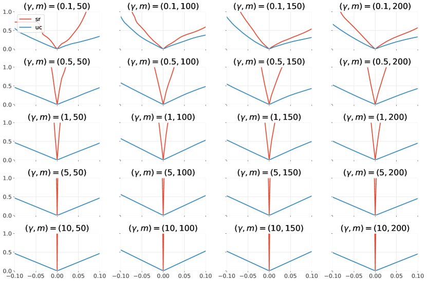
(a) Lipschitzness: $\lambda-\bar{\lambda}_{\text{best}}$ vs. $\|\bar{x}(\lambda)-\bar{x}(\bar{\lambda}_{\text{best}})\|$.

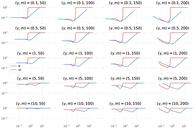
(b) Relative error as a function of $\lambda$ with log-log axis scaling.

Figure 3: Effect of noise scale on error sensitivity for Eq. 1 (sr) and Eq. 18 (uc) faceted by $(\gamma,m)\in\{0.1,0.5,1,5,10\}\times\{50,100,150,200\}$ with $(s,n)=(7,200)$.

In particular, we first investigate empirical Lipschitz behavior of the solution function for Eq. 1 (see Fig. 3(a)). Again, as a reference we compare with that for Eq. 18. In addition, we numerically examine the parameter sensitivity of the relative error for both Eq. 1 and Eq. 18 (see Fig. 3(b)). In both cases, this is done about the empirically optimal parameter values $\bar{\lambda}=\bar{\lambda}_{\text{best}}$. Below, we set $\Lambda:=501$. The logarithmically spaced grid $(\lambda_{i}/\lambda_{*})$ ranges from $10^{-3}$ to $100$ (and includes the point $1$). In this experiment we fix $(s,n)=(7,200)$ and use $\gamma\in\{0.1,0.5,1,5,10\}$, $m\in\{50,100,150,200\}$. Plotted results are depicted in $5\times 4$ grids with each grid cell corresponding to a $(\gamma,m)$ pair.

We readily observe from Fig. 3(a) that for any selected pairing of $(\gamma,m)$, the empirical Lipschitzness of Eq. 1 is worse than that of Eq. 18. Interestingly, we observe that increasing noise scale tends to worsen the empirical Lipschitz behavior of Eq. 1, while it remains (locally) similar for Eq. 18 about the selected reference value.

In Fig. 3(b) we compare the relative errors of each program as a function of $\lambda$. We observe in Fig. 3(b) that, for $m$ fixed, $\bar{\lambda}_{\text{best}}^{\text{SR}}$ is generally less sensitive to variation in $\gamma$ than is $\bar{\lambda}_{\text{best}}^{\text{UC}}$. This observation is consistent with the “tuning robustness” property characteristic of Eq. 1 (cf. Fig. 2(a)). From Fig. 3, we observe for all choices of $(\gamma,m)$ that Eq. 1 is more sensitive to its parameter choice than Eq. 18, again consistent with a comparison of the Lipschitz upper bounds (cf. §​ 6.1).

7 Numerical investigation of our SR-LASSO theory

We present numerical simulations supporting the theoretical results of the previous sections pertaining to solution uniqueness and local Lipschitz moduli. Specifically, we examine the satisfiability of 1 in §​ 7.1 with a graphical demonstration of Theorem 3.7, visualizing for a given set of parameters when Theorem 3.7(ii) holds as a function of $\lambda$. We investigate the tightness of the Lipschitz bound Eq. 17 under 3 in §​ 7.2. Refer to §​ 6.2.1 for an overview of implementation details and relevant notation. For greater detail beyond this, refer to our code repository [13].

7.1 Empirical investigation of uniqueness sufficiency

We begin with an empirical investigation of when the sufficient conditions for uniqueness hold, serving to establish an intuitive understanding of the behavior underlying Theorem 3.7. To this end, we fix a dual pair $(\bar{x},\bar{y})$ for Eq. 1 (i.e., $\bar{x}$ solves Eq. 1 and $\bar{y}$ solves Eq. 8; see Proposition 3.1) and numerically solve the convex program

(22) $$\min_{z\in\mathbb{R}^{m}}\|A_{I^{C}}^{\top}(\bar{y}+z)\|_{\infty}\text{\quad s.t.\quad}[A_{I}\;\bar{y}]^{\top}z=0.$$

We denote the optimal value of the program by $Z^{*}$ and any solution to the program by $\bar{z}$. Then, 1(ii) is satisfied if $Z^{*}<\lambda$. We visualize $Z^{*}$ as a function of $\lambda$ in Fig. 4

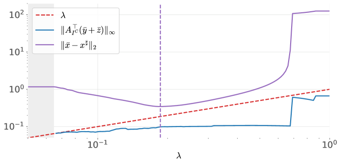
Figure 4: Visualizing uniqueness sufficiency for $(m,n,s,\gamma)=(100,200,2,0.1)$. Upper solid line: error $\|\bar{x}(\lambda)-x^{\sharp}\|_{2}$ where $\bar{x}(\lambda)$ solves Eq. 1. Lower solid line: empirical version of 1(ii) that partially suffices for uniqueness, $\|A_{I^{C}}^{\top}\bar{y}\|_{\infty}$, where $\bar{y}$ solves Eq. 8 and $\bar{z}$ solves Eq. 22. Grey shaded vertical rectangles correspond with $\lambda$ for which $Z^{*}=\infty$. Diagonal dashed line $y=\lambda$ serves as reference for lower solid line. Horizontal position of vertical dashed line denotes $\bar{\lambda}^{\text{SR}}_{\text{best}}$.

by plotting $Z^{*}=Z^{*}(\lambda)$ and the diagonal line “$y=\lambda$”. The former line is given by the lower solid line, the latter by the diagonal dashed line. The upper solid line corresponds to the error $\|\bar{x}(\lambda)-x^{\sharp}\|_{2}$. The horizontal position of the vertical dashed line indicates $\bar{\lambda}_{\text{best}}^{\text{SR}}$ The plot is shown on a log-log scale. Above, the numerical solution for $Z^{*}$ was computed using CVXPY v1.2 [7, 22] with the MOSEK solver [34]. Values of $\lambda$ for which $Z^{*}=\infty$ are shown as grey shaded vertical rectangles. The relative error between the primal Eq. 1 and dual Eq. 8 optimal values was $8.88\times 10^{-7}$, meaning that the two are comfortably within numerical tolerance, given the optimization parameter settings.

In addition, we present a heatmap in Fig. 5

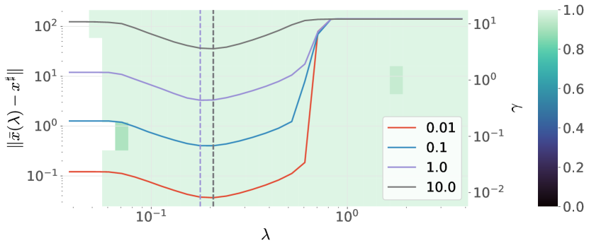
Figure 5: Background: uniqueness sufficiency heatmap displaying the proportion of $20$ independent trials for which $\|A_{I^{C}}^{\top}(\bar{y}+\bar{z})\|_{\infty}<\lambda$ is satisfied, where $\bar{y}$ solves Eq. 8 and $\bar{z}$ solves Eq. 22. Voxels correspond to $\lambda$ (horizontal axis) and noise scale $\gamma$ (right axis). White regions: no data. Foreground: error $\|\bar{x}(\lambda)-x^{\sharp}\|_{2}$ (left axis) as a function of $\lambda$ for four choices of the noise scale $\gamma$ (see legend). Vertical dashed lines are drawn at $\bar{\lambda}_{\text{best}}$ for each.

demonstrating the relative frequency that the sufficient condition for uniqueness is satisfied for a range of $31\times 7$ logarithmically spaced parameter values $(\lambda,\gamma)\in[0.1,10]\times[0.01,10]$ (horizontal and right axis, respectively). Each pixel displays a mean of $20$ independent repetitions with $1$ corresponding to the sufficient condition being satisfied for all trials; $0$ corresponding to the condition being satisfied for none of the trials. Apart from the changing noise scale $\gamma$, the signal/measurement model is the same as described above. We also compute $Z^{*}=Z^{*}(i,\gamma,\lambda)$ as described above, where $i\in[20]$ is the trial number. White regions in the heatmap correspond none of the $20$ trials yielding an inexact solution, violating a tenet of our theory that $A\bar{x}\neq b$. Superposed on the heatmap is a plot of the recovery error (left vertical axis) as a function of $\lambda$ for $4$ of the values of $\gamma$ (see legend). Fig. 5 reveals a sizable region where the sufficient condition for uniqueness is empirically assured. Moreover, this region encompasses all $\bar{\lambda}_{\text{best}}$ values with a comfortable margin, and it is relatively insensitive to $\gamma$.

7.2 Empirical investigation of Lipschitz upper bound

Finally, we compare the Lipschitz upper bound Eq. 17 to the empirical Lipschitz quantity $\|\bar{x}(\lambda)-\bar{x}(\bar{\lambda})\|$ where $\bar{\lambda}:=\bar{\lambda}_{\text{best}}$. To this end, we investigate two settings where the dimensional parameters are varied, with results displayed in Fig. 6.

(a) Variation in $(m,s)$.

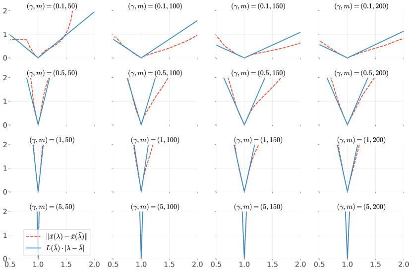
(b) Variation in $(m,\gamma)$.

Figure 6: Effect of varying dimensional parameters on the Lipschitz upper bound: $L(\bar{\lambda})|\lambda-\bar{\lambda}|$ vs. the empirical Lipschitz quantity $\|\bar{x}(\lambda)-\bar{x}(\bar{\lambda})\|$ as a function of $\lambda_{\text{nmz}}$. $L(\bar{\lambda})$ is computed as in Eq. 17. Top: $(m,s)\in\{50,100,150,200\}\times\{3,7,15\}$; Bottom: $(m,\gamma)\in\{50,100,150,200\}\times\{0.1,0.5,1,5\}$.

Throughout, we choose $n=200$. In the first experiment, shown in Fig. 6(a), we set $\gamma=0.1$ and choose $(m,s)\in\{50,100,150,200\}\times\{3,7,15\}$; in the second, shown in Fig. 6(b), we set $s=7$ and choose $(m,\gamma)\in\{50,100,150,200\}\times\{0.1,0.5,1,5\}$. Generally, we observe that the Lipschitz upper bound $L(\bar{\lambda})$ given by Eq. 17 is a tight local approximation to the true Lipschitz behavior of the solution $\bar{x}(\lambda)$ about $\bar{\lambda}$.

8 Conclusion

In this paper, we studied the Square Root LASSO (SR-LASSO) Eq. 1. We established sufficient conditions for its well-posedness, namely 1, and linked it to two stronger regularity conditions, the intermediate condition 2 and the strong condition 3, respectively. The intermediate condition is shown to imply local Lipschitzness and directional differentiability of the solution map as a function of the right-hand side and the tuning parameter (around a reference point); the strong condition, in turn, guarantees continuous differentiability of said solution map. We then leveraged these results to compare the SR-LASSO to its close relative, the (unconstrained) LASSO from a theoretical perspective. This comparison suggests that the celebrated robustness of optimal parameter tuning to noise of the SR-LASSO comes at the price of elevated sensitivity of the solution map to the tuning parameter itself. Our numerical experiments confirmed the presence of this robustness-sensitivity trade off for parameter tuning, and illustrated the sharpness of our Lipschitz bounds and the validity of the main assumptions upon which the theory relies on.

We conclude by discussing possible extensions of this work and open problems: although we focused on the dependence of the solution map in $b$ and $\lambda$, we point out that it is straightforward (at the cost of more computational overhead) to extend all stability results to the case where also the design matrix $A$ is a parameter. Moreover, similarly to [14], our results could be explicitly applied to compressed sensing theory by combining our Lipschitz bounds with explicit estimates of the sparsity of SR-LASSO solutions [25]. Finally, in the LASSO case it is known [49] that the analogous sufficient condition to 1 is also necessary for uniqueness. At this point, whether this is also true for the SR-LASSO, is an open question and we challenge the reader to clarify it.

Appendix A Proof of shrinking property

Here, we furnish proof of Lemma 3.10. Note that, for $f,g:\mathbb{R}^{n}\to\overline{\mathbb{R}}$, their infimal convolution [37] is denoted by $(f\mathbin{\hash}g)(x):=\inf_{u}f(x-u)+g(u)$.

Proof A.1 (Proof of Lemma 3.10).

The (primal) problem defining $p^{*}$ reads

(23) $$\min_{z\in\mathbb{R}^{m}}\|B^{\top}(\bar{y}+z)\|_{\infty}+\delta_{\varepsilon\mathbb{B}\cap\mathcal{T}}(z).$$

The minimum is attained due to compactness and lower semicontinuity. Now, set $f:=\delta_{\varepsilon\mathbb{B}\cap\mathcal{T}}$ and $g:=\|B^{\top}\bar{y}+(\cdot)\|_{\infty}.$ With $\operatorname{d}_{\mathcal{T}^{\perp}}$, the Euclidean distance to $\mathcal{T}^{\perp}$, we find

$$f^{*}(u) =\delta_{\varepsilon\mathbb{B}\cap\mathcal{T}}^{*}(u)$$

$$=(\delta_{\varepsilon\mathbb{B}}+\delta_{\mathcal{T}})^{*}(u)$$

$$=(\sigma_{\varepsilon\mathbb{B}}\mathbin{\hash}\sigma_{\mathcal{T}})(u)$$

$$=\inf_{y}\varepsilon\|y\|+\delta_{\mathcal{T}^{\perp}}(u-y)$$

$$=\varepsilon\operatorname{d}_{\mathcal{T}^{\perp}}(u),$$

where in the third line, we have used [37, Theorem 16.4] combined with the fac that $0\in(\operatorname{int}\varepsilon\mathbb{B})\cap\mathcal{T}$. We also have $g^{*}(u)=\delta_{\mathbb{B}_{1}}(u)-\left\langle B^{\top}\bar{y},\,u\right\rangle$. Hence, with $\phi(u):=-\left\langle B^{\top}\bar{y},\,u\right\rangle-\varepsilon\operatorname{d}_{\mathcal{T}^{\perp}}(Bu)$, the (Fenchel-Rockafellar) dual problem of Eq. 23 is

(24) $$\max-f^{*}(Bu)-g^{*}(-u)\qquad\iff\qquad\max_{u\in\mathbb{B}_{1}}\phi(u).$$

Now, observe that (see e.g., [30]) $-\left\langle B^{\top}\bar{y},\,u\right\rangle\leq\|B^{\top}\bar{y}\|_{\infty}\|u\|_{1}.$ Hence, for every feasible point of Eq. 24, we have

(25) $$\phi(u)\leq\|B^{\top}\bar{y}\|_{\infty}-\varepsilon\operatorname{d}_{\mathcal{T}^{\perp}}(Bu).$$

We claim that $\phi(u)<\|B^{\top}\bar{y}\|_{\infty}$ for all $u\in\mathbb{B}_{1}$. Indeed, assume to the contrary the existence of a $\hat{u}$ feasible for Eq. 24 such that $\phi(\hat{u})=\|B^{\top}\bar{y}\|_{\infty}$. Then Eq. 25 implies

$$\operatorname{d}_{\mathcal{T}^{\perp}}(B\hat{u})=0\qquad \iff\qquad B\hat{u}\in\mathcal{T}^{\perp}=\mathbb{R}\cdot\{\bar{y}\}+\mathrm{rge}\,C$$

$$\implies\qquad\bar{y}\in\mathrm{rge}\,C+\mathrm{rge}\,B=\mathrm{rge}\,[B\;C],$$

contradicting an assumption of the lemma. Consequently, since the dual problem admits a solution, $\bar{u}$ say, we find by strong duality that $p^{*}=\phi(\bar{u})<\|B^{\top}\bar{y}\|_{\infty}.$

Appendix B Proof of analytic solution formula under 2

Here, we provide the proof for the analytic expression for the (unique) solution under the intermediate condition from 2.

Proof B.1 (Proof of Proposition 3.13).

By assumption, the dual problem Eq. 8 has a unique solution $\bar{y}=\frac{b-A\bar{x}}{\|A\bar{x}-b\|}.$ Therefore, using the optimality conditions for $\bar{x}$, there exists a unique subgradient $v\in\partial\|\cdot\|_{1}(\bar{x})$ such that $A^{\top}\bar{y}=\lambda v$. By definition of $v$ and the fact that $I\subseteq J$, we have $\|\bar{x}\|_{1}=\left\langle v,\,\bar{x}\right\rangle=\left\langle v_{J},\,\bar{x}_{J}\right\rangle$. We thus rewrite the strong duality expression Proposition 3.1(b)(ii) as

(26) $$\|A\bar{x}-b\|=\left\langle b,\,\bar{y}\right\rangle-\lambda\left\langle v_{J},\,\bar{x}_{J}\right\rangle.$$

Using Corollary 3.3(b), we can rewrite the optimality conditions as $A^{\top}(b-A\bar{x})=\lambda\|A\bar{x}-b\|v$. Restricting to $J$ and using Eq. 26 gives

$$A_{J}^{\top}(b-A_{J}\bar{x}_{J})=\lambda\left(\left\langle b,\,\bar{y}\right\rangle-\lambda\left\langle v_{J},\,\bar{x}_{J}\right\rangle\right)v_{J}=\lambda\left\langle b,\,\bar{y}\right\rangle v_{J}-\lambda^{2}v_{J}v_{J}^{\top}\bar{x}_{J}.$$

After rearranging, we obtain $\left(A_{J}^{\top}A_{J}-\lambda^{2}v_{J}v_{J}^{\top}\right)\bar{x}_{J}=A_{J}^{\top}b-\lambda\left\langle b,\,\bar{y}\right\rangle v_{J}$. It remains to verify that the matrix $A_{J}^{\top}A_{J}-\lambda^{2}v_{J}v_{J}^{\top}$ satisfies the desired identity and is invertible. To this end, the $J$-restricted optimality conditions $A_{J}^{\top}\bar{y}=\lambda v_{J}$ imply

$$A_{J}^{\top}A_{J}-\lambda^{2}v_{J}v_{J}^{\top}=A_{J}^{\top}\left(\operatorname{\mathbb{I}}-\bar{y}\bar{y}^{\top}\right)A_{J}.$$

To obtain invertibility of this matrix, we apply Lemma 2.1, using that $A_{J}$ has full column rank and $\bar{y}\notin\mathrm{rge}\,A_{J}$ (because $b\notin\mathrm{rge}\,A_{J}$). In particular,

$$\bar{x}_{J}=B\left(A_{J}^{\top}b-\lambda\left\langle b,\,\bar{y}\right\rangle v_{J}\right),\qquad B:=\left[A_{J}^{\top}(\operatorname{\mathbb{I}}-\bar{y}\bar{y}^{\top})A_{J}\right]^{-1}.$$

An explicit expression for $B$ is provided by Lemma 2.1. Notice that uniqueness of $\bar{y}$ implies that of $v$ and $J$, and hence too of $x_{J}$. Finally, $x_{J^{C}}\equiv 0$ because $I\subseteq J$. Hence,

$$\bar{x}=L_{J}\left(B\left(A_{J}^{\top}b-\left\langle b,\,\bar{y}\right\rangle A_{J}^{\top}\bar{y}\right)\right)=L_{J}\left(BA_{J}^{\top}(\operatorname{\mathbb{I}}-\bar{y}\bar{y}^{\top})b\right).$$

Appendix C Auxiliary results

Lemma C.1.

Let $\bar{A}\in\mathbb{R}^{m\times n}$, $\bar{b}\in\mathbb{R}^{m}$, $\bar{x}\in\mathbb{R}^{n}$ such that $\bar{A}\bar{x}\neq\bar{b}$ and let $\bar{\lambda}>0$. Then, there exists a neighborhood $U$ of $(\bar{A},\bar{b},\bar{\lambda},\bar{x})$ such that the function $\phi:U\to\mathbb{R}^{n}$,

$$\phi(A,b,\lambda,x):=\frac{A^{\top}(Ax-b)}{\lambda\|Ax-b\|},$$

is well defined and continuously differentiable on $U$ with partial derivatives:

• $D_{A}\phi(A,b,\lambda,x)(W)=\frac{1}{\lambda\|Ax-b\|}\left[(A^{\top}W+W^{\top}A)x-W^{\top}b-\frac{A^{\top}(Ax-b)(Ax-b)^{\top}Wx}{\|Ax-b\|^{2}}\right]$;

• $D_{b}\phi(A,b,\lambda,x)=-\frac{1}{\lambda\|Ax-b\|}\left[\frac{A^{\top}-A^{\top}(Ax-b)(Ax-b)^{\top}}{\|Ax-b\|^{2}}\right]$;

• $D_{\lambda}\phi(A,b,\lambda,x)=-\frac{1}{\lambda^{2}\|Ax-b\|}A^{\top}(Ax-b)$;

• $D_{x}\phi(A,b,\lambda,x)=\frac{1}{\lambda\|Ax-b\|}\left[A^{\top}A-A^{\top}\frac{Ax-b}{\|Ax-b\|}\frac{(Ax-b)^{\top}}{\|Ax-b\|}A\right]$.

References

- [1] B. Adcock, A. Bao, and S. Brugiapaglia, Correcting for unknown errors in sparse high-dimensional function approximation, Numerische Mathematik, 142 (2019), pp. 667–711.
- [2] B. Adcock, S. Brugiapaglia, N. Dexter, and S. Moraga, Deep neural networks are effective at learning high-dimensional Hilbert-valued functions from limited data, in Proceedings of the 2nd Mathematical and Scientific Machine Learning Conference, J. Bruna, J. Hesthaven, and L. Zdeborova, eds., vol. 145 of Proceedings of Machine Learning Research, PMLR, 16–19 Aug 2022, pp. 1–36, https://proceedings.mlr.press/v145/adcock22a.html.
- [3] B. Adcock, S. Brugiapaglia, and M. King-Roskamp, Do log factors matter? on optimal wavelet approximation and the foundations of compressed sensing, Foundations of Computational Mathematics, 22 (2022), pp. 99–159.
- [4] B. Adcock, S. Brugiapaglia, and C. G. Webster, Sparse Polynomial Approximation of High-Dimensional Functions, vol. 25, SIAM, 2022.
- [5] B. Adcock and N. Dexter, The gap between theory and practice in function approximation with deep neural networks, SIAM Journal on Mathematics of Data Science, 3 (2021), pp. 624–655.
- [6] B. Adcock and A. C. Hansen, Compressive Imaging: Structure, Sampling, Learning, Cambridge University Press, 2021.
- [7] A. Agrawal, R. Verschueren, S. Diamond, and S. Boyd, A rewriting system for convex optimization problems, Journal of Control and Decision, 5 (2018), pp. 42–60.
- [8] P. Babu, Spectral analysis of nonuniformly sampled data and applications., PhD thesis, Uppsala University, 2012.
- [9] P. Babu and P. Stoica, Connection between SPICE and square-root LASSO for sparse parameter estimation, Signal Processing, 95 (2014), pp. 10–14.
- [10] A. Belloni, V. Chernozhukov, and L. Wang, Square-root LASSO: pivotal recovery of sparse signals via conic programming, Biometrika, 98 (2011), pp. 791–806.
- [11] A. Belloni, V. Chernozhukov, and L. Wang, Pivotal estimation via square-root lasso in nonparametric regression, The Annals of Statistics, 42 (2014), pp. 757–788.
- [12] A. Berk, On LASSO parameter sensitivity, PhD thesis, University of British Columbia, 2021.
- [13] A. Berk, S. Brugiapaglia, and T. Hoheisel, Code repository. https://github.com/asberk/srlasso_revolutions.
- [14] A. Berk, S. Brugiapaglia, and T. Hoheisel, LASSO reloaded: a variational analysis perspective with applications to compressed sensing, arXiv preprint arXiv:2205.06872, (2022).
- [15] A. Berk, Y. Plan, and Ö. Yılmaz, On the best choice of LASSO program given data parameters, IEEE Transactions on Information Theory, 68 (2021), pp. 2573–2603.
- [16] A. Berk, Y. Plan, and Ö. Yılmaz, Sensitivity of minimization to parameter choice, Information and Inference: A Journal of the IMA, 10 (2021), pp. 397–453.
- [17] P. J. Bickel, Y. Ritov, and A. B. Tsybakov, Simultaneous analysis of Lasso and Dantzig selector, The Annals of Statistics, 37 (2009), pp. 1705–1732.
- [18] J. Bolte, E. Pauwels, and A. Silvetti-Falls, Nonsmooth implicit differentiation for machine-learning and optimization, Advances in Neural Information Processing Systems, 34 (2021).
- [19] J. Bolte, E. Pauwels, and A. Silvetti-Falls, Differentiating nonsmooth solutions to parametric monotone inclusion problems, arXiv preprint arXiv:2212.07844, (2022).
- [20] F. Bunea, J. Lederer, and Y. She, The group square-root lasso: Theoretical properties and fast algorithms, IEEE Transactions on Information Theory, 60 (2013), pp. 1313–1325.
- [21] M. J. Colbrook, V. Antun, and A. C. Hansen, The difficulty of computing stable and accurate neural networks: On the barriers of deep learning and smale’s 18th problem, Proceedings of the National Academy of Sciences, 119 (2022), p. e2107151119.
- [22] S. Diamond and S. Boyd, CVXPY: A Python-embedded modeling language for convex optimization, Journal of Machine Learning Research, 17 (2016), pp. 1–5.
- [23] D. L. Donoho, Compressed sensing, IEEE Transactions on Information Theory, 52 (2006), pp. 1289–1306.
- [24] A. L. Dontchev and R. T. Rockafellar, Implicit Functions and Solution Mappings, Springer Series in Operations Research and Financial Engineering, Springer, New York, NY, 2nd ed., 2014.
- [25] S. Foucart, The sparsity of LASSO-type minimizers, Applied and Computational Harmonic Analysis, 62 (2023), pp. 441–452.
- [26] M. P. Friedlander, A. Goodwin, and T. Hoheisel, From perspective maps to epigraphical projections, Mathematics of Operations Research, (2022).
- [27] J. C. Gilbert, On the solution uniqueness characterization in the L1 norm and polyhedral gauge recovery, Journal of Optimization Theory and Applications, 172 (2017), pp. 70–101.
- [28] C. R. Harris, K. J. Millman, S. J. van der Walt, R. Gommers, P. Virtanen, D. Cournapeau, E. Wieser, J. Taylor, S. Berg, N. J. Smith, R. Kern, M. Picus, S. Hoyer, M. H. van Kerkwijk, M. Brett, A. Haldane, J. F. del Río, M. Wiebe, P. Peterson, P. Gérard-Marchant, K. Sheppard, T. Reddy, W. Weckesser, H. Abbasi, C. Gohlke, and T. E. Oliphant, Array programming with NumPy, Nature, 585 (2020), pp. 357–362, https://doi.org/10.1038/s41586-020-2649-2, https://doi.org/10.1038/s41586-020-2649-2.
- [29] T. Hoheisel and E. Paquette, Uniqueness in nuclear norm minimization: Flatness of the nuclear norm sphere and simultaneous polarization, Journal of Optimization Theory and Applications, (2023).
- [30] R. A. Horn and C. R. Johnson, Matrix Analysis, Cambridge University Press, Cambridge, UK, 2nd ed., 2012, https://doi.org/10.1017/9781139020411.
- [31] S. Mohammad-Taheri and S. Brugiapaglia, The greedy side of the LASSO: New algorithms for weighted sparse recovery via loss function-based orthogonal matching pursuit, arXiv preprint arXiv:2303.00844, (2023).
- [32] B. Mordukhovich, Variational Analysis and Generalized Differentiation. I: Basic Theory, vol. 330 of Grundlehren der mathematischen Wissenschaften, Springer-Verlag Berlin, Heidelberg, Germany, 2006.
- [33] B. Mordukhovich, Variational Analysis and Applications, Springer Monographs in Mathematics book series, Springer International Publishing AG, 2018.
- [34] MOSEK ApS, MOSEK Optimizer API for Python 9.3.21, 2019, https://docs.mosek.com/9.3/pythonapi/index.html.
- [35] H. B. Petersen and P. Jung, Robust instance-optimal recovery of sparse signals at unknown noise levels, Information and Inference: A Journal of the IMA, 11 (2022), pp. 845–887.
- [36] V. Pham and L. El Ghaoui, Robust sketching for multiple square-root LASSO problems, in Artificial Intelligence and Statistics, PMLR, 2015, pp. 753–761.
- [37] R. T. Rockafellar, Convex Analysis, vol. 18, Princeton University Press, Princeton, NJ, 1970.
- [38] R. T. Rockafellar and R. J.-B. Wets, Variational Analysis, vol. 317 of Grundlehren der mathematischen Wissenschaften, Springer-Verlag Berlin, Heidelberg, Germany, 1998.
- [39] Y. Shen, B. Han, and E. Braverman, Stable recovery of analysis based approaches, Applied and Computational Harmonic Analysis, 39 (2015), pp. 161–172.
- [40] P. Stoica, P. Babu, and J. Li, New method of sparse parameter estimation in separable models and its use for spectral analysis of irregularly sampled data, IEEE Transactions on Signal Processing, 59 (2010), pp. 35–47.
- [41] B. Stucky and S. Van de Geer, Sharp oracle inequalities for square root regularization, Journal of Machine Learning Research, 18 (2017), pp. 1–29.
- [42] T. Sun and C.-H. Zhang, Scaled sparse linear regression, Biometrika, 99 (2012), pp. 879–898.
- [43] X. Tian, J. R. Loftus, and J. E. Taylor, Selective inference with unknown variance via the square-root lasso, Biometrika, 105 (2018), pp. 755–768.
- [44] R. J. Tibshirani, Regression shrinkage and selection via the lasso, Journal of the Royal Statistical Society: Series B (Methodological), 58 (1996), pp. 267–288.
- [45] R. J. Tibshirani, The Lasso problem and uniqueness, Electronic Journal of Statistics, 7 (2013), pp. 1456–1490.
- [46] S. Vaiter, C. Deledalle, J. Fadili, G. Peyré, and C. Dossal, Low complexity regularization of linear inverse problems, Applied and Numerical Harmonic Analysis, Birkhäuser/Springer, 2015, pp. 103–153.
- [47] S. Vaiter, C. Deledalle, J. Fadili, G. Peyré, and C. Dossal, The degrees of freedom of partly smooth regularizers, 69 (2017), pp. 791–832.
- [48] S. Van de Geer, Estimation and testing under sparsity, Lecture Notes in Mathematics, Springer Cham, Switzerland, 2016.
- [49] H. Zhang, W. Yin, and L. Cheng, Necessary and sufficient conditions of solution uniqueness in -norm minimization, Journal of Optimization Theory and Applications, 164 (2015), pp. 109–122.