Adjusted Wasserstein Distributionally Robust Estimator in Statistical Learning

Abstract

We propose an adjusted Wasserstein distributionally robust estimator—based on a nonlinear transformation of the Wasserstein distributionally robust (WDRO) estimator in statistical learning. The classic WDRO estimator is asymptotically biased, while our adjusted WDRO estimator is asymptotically unbiased, resulting in a smaller asymptotic mean squared error. Meanwhile, the proposed adjusted WDRO has an out-of-sample performance guarantee. Further, under certain conditions, our proposed adjustment technique provides a general principle to de-bias asymptotically biased estimators. Specifically, we will investigate how the adjusted WDRO estimator is developed in the generalized linear model, including logistic regression, linear regression, and Poisson regression. Numerical experiments demonstrate the favorable practical performance of the adjusted estimator over the classic one.

Keywords: distributionally robust optimization; asymptotic normality; Wasserstein distance; unbiased estimator; generalized linear model

1 Introduction

Wasserstein distributionally robust optimization (WDRO) has appeared as a promising tool to achieve “robust” decision-making (Mohajerin Esfahani and Kuhn, 2018; Blanchet and Murthy, 2019; Gao and Kleywegt, 2022). WDRO has attracted intense research interest in the past few years. It is well-known that WDRO admits tractable reformulations (Mohajerin Esfahani and Kuhn, 2018) and has a powerful out-of-sample performance guarantee (Gao, 2022). People also have been actively exploring its applications in financial portfolio selection (Blanchet et al., 2022a), statistical learning (Chen and Paschalidis, 2018; Shafieezadeh-Abadeh et al., 2019), neural networks (Sinha et al., 2018), automatic control (Yang, 2020), transportation (Carlsson et al., 2018), and energy systems (Wang et al., 2018), among others.

WDRO can be applied in statistical learning (Chen and Paschalidis, 2018; Kuhn et al., 2019; Nguyen et al., 2022). In general, the statistical learning model can be written as the following optimization problem:

$$\min_{\beta\in B}\mathbb{E}_{P_{\ast}}\left[L(f(\mathbf{X},\beta),Y)\right],$$

where $\mathbf{X}\in\Omega\subset\mathbb{R}^{d}$ denotes the feature variable, $Y$ denotes the label variable, $P_{\ast}$ is the underlying data-generating distribution of $(\mathbf{X},Y)$, $f(\cdot,\beta)$ is the hypothesis function parameterized by $\beta\in B\subset\mathbb{R}^{d}$, $B$ is a compact convex set, and $L(\cdot,\cdot)$ is the loss function. Considering the true data-generating distribution $P_{\ast}$ is usually unknown, the empirical risk minimization can be applied to estimate the ground-truth hypothesis function $f(\cdot,\beta_{\ast})$ parameterized by $\beta_{\ast}\not=0$. However, the empirical risk minimization estimators are sensitive to perturbations and suffer from overfitting (Smith and Winkler, 2006; Shalev-Shwartz and Ben-David, 2014). To obtain robust estimators with desirable generalization abilities, distributionally robust optimization is proposed, which minimizes the worst-case expected loss among an ambiguity set $\mathcal{U}$ of distributions to hedge against data perturbation. In this paper, we are interested in the Wasserstein ambiguity set, and then the resulting problem is the so-called Wasserstein distributionally robust optimization. The Wasserstein ambiguity is defined as the ball centered at the empirical distribution $\mathbb{P}_{N}$ and contains all distributions close to $\mathbb{P}_{N}$ in the sense of the Wasserstein distance. We denote the WDRO estimators—the solutions to the WDRO problem—by $\beta_{n}^{DRO}$. More details will be stated in Section 4.

The asymptotic distribution of the WDRO estimator $\beta_{n}^{DRO}$ can be obtained under certain regularity conditions. In particular, the convergence in distribution implies that the WDRO estimator $\beta^{DRO}_{n}$ has an asymptotic bias, which may result in inaccurate estimation of the ground-truth parameter $\beta_{\ast}$. Inspired by this phenomenon, we provide a general adjustment technique to de-bias the asymptotically biased estimators, where we also discuss the asymptotic behavior of different transformations on the estimators.

Applying the proposed adjustment technique to the WDRO problem, we obtain the adjusted WDRO estimator, denoted by $\beta_{n}^{ADRO}$. It will be shown that the adjusted WDRO estimator $\beta_{n}^{ADRO}$ could be computed exactly simply using the given samples and the value of the classic WDRO estimator $\beta_{n}^{DRO}$, making it convenient to apply the proposed technique. Also, the existence and the asymptotic unbiasedness of the adjusted WDRO estimator $\beta_{n}^{ADRO}$ could be promised under mild conditions, enabling broad applications of the proposed technique. In addition, the out-of-sample performance guarantee of the proposed estimator $\beta^{ADRO}_{n}$ can be derived, demonstrating that the proposed estimator $\beta^{ADRO}_{n}$ inherits the generalization capacity of the WDRO estimator.

Since the generalized linear model includes multiple widely-used regression models and is easy to interpret and implement, we will articulate how to apply the adjustment strategy in the setting of the generalized linear model, including linear regression, logistic regression, and Poisson regression. Then, we carry out the numerical experiments in the generalized linear model. Our numerical experiments illustrate that the proposed estimator $\beta_{n}^{ADRO}$ has a superior performance even if the sample size is relatively small.

1.1 Related Work

We review the existing work related to the proposed adjusted WDRO estimator. WDRO is broadly applied to solve parameter estimation problems (Shafieezadeh Abadeh et al., 2015; Kuhn et al., 2019; Aolaritei et al., 2022; Nguyen et al., 2022). Multiple algorithms have been developed (Luo and Mehrotra, 2019; Li et al., 2019; Blanchet et al., 2022c) and can be applied to compute the parameter estimators in the WDRO framework. While intense work focuses on adapting WDRO to different machine learning problems, deriving the tractable reformulations, and solving the WDRO problems efficiently, the statistical properties of WDRO estimators have been investigated in recent few years, e.g., Blanchet et al. (2022b, 2021), evaluating the behavior of WDRO through the lens of statistics. In the aforementioned paper, the asymptotic distribution of the WDRO estimator is proven to be normal, and the confidence region is proposed based on the corresponding asymptotic results. While they focus on unsupervised settings, we extend the results to supervised statistical learning, especially in the setting of the generalized linear model. Notably, the asymptotic biasedness of the WDRO estimator has been mentioned in Blanchet et al. (2022b). However, we are the first to propose a nonlinear transformation to overcome this shortcoming. Furthermore, the proposed estimator is more accurate in the asymptotic sense because the estimator also has an asymptotically smaller mean squared error. In addition, the generalization bounds, i.e., the upper confidence bounds on the out-of-sample error, have been established to guarantee the out-of-sample performance of the WDRO estimator (Mohajerin Esfahani and Kuhn, 2018; Shafieezadeh-Abadeh et al., 2019; Gao, 2022; Wu et al., 2022). Since the proposed adjusted WDRO estimator is transformed from the classic WDRO estimator, we can also develop the generalization bounds for the associated adjusted WDRO estimator.

1.2 Organization of this Paper

The remainder of this paper is organized as follows. In Section 2, we introduce the adjustment technique that could de-bias the general asymptotically biased estimators under certain conditions. In Section 3, we discuss the asymptotic behavior of the WDRO problem. In Section 4, we give the formulation of the adjusted WDRO estimator in statistical learning. In Section 5, we show how to develop the adjusted WDRO estimators in the generalized linear model. Numerical experiments are conducted and analyzed in Section 6. The proofs are relegated to the appendix whenever possible.

2 Adjustment Technique

In this section, we first discuss the properties of transformations on the asymptotically biased estimators, based on which we provide a general strategy to de-bias the asymptotically biased estimators under certain conditions. The proposed adjustment technique will be further illustrated in detail in the WDRO setting in Section 4.

Suppose the estimator $\beta_{n}\in\mathbb{R}^{d}$ is obtained by the following parameter-estimation procedure

$$\beta_{n}\in\arg\min_{\beta}l(\mathbb{P}_{n},\beta),$$

where $l$ is the loss and depends on the empirical distribution $\mathbb{P}_{n}$ and parameter $\beta$. Also, suppose that the estimator $\beta_{n}$ has the following convergence in distribution:

$$\sqrt{n}(\beta_{n}-\beta_{\ast})\Rightarrow\mathcal{N}(f(\beta_{\ast}),D),$$ (1)

where $\Rightarrow$ means “converge in distribution”, $D\in\mathbb{R}^{d\times d}$, $f:\mathbb{R}^{d}\mapsto\mathbb{R}^{d}$ and $\beta_{\ast}\in\mathbb{R}^{d}$ is the ground-truth parameter. We focus on the scenario when $f\not=0$.

For the estimator $\beta_{n}$ with the limiting distribution in (1), our goal is to look for some transformation $\phi_{n}(\cdot)$ to obtain a more accurate estimation of $\beta_{\ast}$ in the asymptotic sense. The following proposition states that the “best” transformations have a unique formulation.

Proposition 1

Suppose $\beta_{n}$ is the estimator of $\beta_{\ast}$ and has the following convergence in distribution:

$$\sqrt{n}(\beta_{n}-\beta_{\ast})\Rightarrow\mathcal{N}(f(\beta_{\ast}),D).$$

Assume the transformation $\phi_{n}(\cdot)$ is differentiable satisfying $\phi_{n}^{\prime}(\beta_{\ast})\to\phi^{\prime}(\beta_{\ast})$, where $\phi$ is differentiable, and $\phi_{n}^{\prime}$ and $\phi^{\prime}$ are the gradients of $\phi_{n}$ and $\phi$. The least asymptotic mean squared error of $\phi_{n}(\beta_{n})$ is $\mathrm{tr}(D)$, which is obtained if and only if $\phi_{n}(\cdot)$ could be written as

$$\phi_{n}(\beta)=\beta-\frac{1}{\sqrt{n}}f(\beta)+o\left(\frac{1}{\sqrt{n}}\right).$$ (2)

In this way, we have that

$$\sqrt{n}(\phi_{n}(\beta_{n})-\beta_{\ast})\Rightarrow\mathcal{N}(0,D).$$

Proposition 1 demonstrates that for the asymptotically biased estimator $\beta_{n}$, to achieve the least asymptotic mean squared error $\mathrm{tr}(D)$, the transformation $\phi_{n}(\cdot)$ must take the formulation (2). Meanwhile, the resulting estimator $\phi_{n}(\beta_{n})$ is asymptotically unbiased.

The transformation $\phi_{n}(\cdot)$ in the formulation (2) is desirable since it could de-bias the asymptotically biased estimator $\beta_{n}$ and achieve the least asymptotic mean squared error $\mathrm{tr}(D)$. However, the transformation $\phi_{n}(\cdot)$ depends on the function $f$, which is usually unknown. For example, in the limiting distribution of the WDRO estimator, $f$ depends on the unknown underlying distribution. In this regard, the function $f$ should be approximated accordingly.

Suppose we have a sequence of functions $f_{n}$ to approximate the function $f$. Our adjustment transformation could be defined in terms of $f_{n}$ based on $\phi_{n}(\cdot)$ in (2). We assume $f_{n}$ could be computed via the empirical distribution $\mathbb{P}_{n}$, and certain conditions should be imposed to $f_{n}$ to promise that the estimator obtained by our adjustment transformation is asymptotically unbiased and could have the mean squared error $\mathrm{tr}(D)$. More details are described in Assumption 2 and Theorem 3.

Before introducing Theorem 3, we state our assumptions of functions $f_{n}$.

Assumption 2

Given function $f$, $f_{n}$ and $\beta_{\ast}$, we assume that

• The function $f_{n}$ is differentiable at $\mathcal{B}(\beta_{\ast})$, where $\mathcal{B}(\beta_{\ast})$ is some neighborhood of $\beta_{\ast}$.

• The sequence $\sup_{\beta\in\mathcal{B}(\beta_{\ast})}\|f^{\prime}_{n}(\beta)\|$ is bounded in probability.

• $f_{n}(\beta_{\ast})\to_{p}f(\beta_{\ast})$, where $\to_{p}$ means “converge in probability”.

Equipped with Assumption 2, we give our main theorem in the following.

Theorem 3 (Adjustement Technique)

Suppose $\beta_{n}$ is the estimator of $\beta_{\ast}$ and has the following convergence in distribution:

$$\sqrt{n}(\beta_{n}-\beta_{\ast})\Rightarrow\mathcal{N}(f(\beta_{\ast}),D).$$

If we have function $f_{n}$ satisfying Assumption 2 and the transformation $\mathcal{A}_{n}(\cdot)$ defined by

$$\mathcal{A}_{n}(\beta_{n})=\beta_{n}-\frac{1}{\sqrt{n}}f_{n}(\beta_{n}),$$

then

$$\sqrt{n}\left(\mathcal{A}_{n}(\beta_{n})-\beta_{\ast}\right)\Rightarrow\mathcal{N}(0,D).$$ (3)

The convergence (3) in Theorem 3 demonstrates that the proposed adjusted estimator $\mathcal{A}_{n}(\beta_{n})$ is asymptotically unbiased and the asymptotic covariance matrix remains unchanged, resulting in a smaller asymptotic means square error $\mathrm{tr}(D)$, which equals the least mean squared error stated in Proposition 1. In this regard, to de-bias the asymptotically biased estimators, one only needs to have a sequence of functions $f_{n}$ satisfying Assumption 2.

2.1 Sequential Delta Method

Notice that the transformations $\phi_{n}$ discussed in Proposition 1 depend on $n$. In this way, when we discuss the asymptotic distribution of $\phi_{n}(\beta_{n})$, the classic delta method is not applicable. To resolve this issue, we have developed a sequential delta method based on the extended continuous mapping theorem (Theorem 1.11.1 in Van der Vaart and Wellner (1996)). The sequential delta method may have an independent research interest, so we state it in the following theorem.

Theorem 4 (Sequential Delta Method)

Let $\phi_{n}$ and $\phi:\mathbb{D}\subset\mathbb{R}^{d}\mapsto\mathbb{R}^{d}$ be functions defined on a subset of $\mathbb{R}^{d}$, differentiable at $\theta$, satisfying $\phi^{\prime}_{n}(\theta)\to\phi^{\prime}(\theta)$, where $\phi^{\prime}$ and $\phi^{\prime}_{n}$ are gradients of the functions $\phi$ and $\phi_{n}$. Let $T_{n}$ be random vectors taking their values in the domain of $\phi$. If $r_{n}(T_{n}-\theta)\Rightarrow\mathcal{N}(\mu,\Sigma)$ for numbers $r_{n}\to\infty$, then $r_{n}(\phi_{n}(T_{n})-\phi_{n}(\theta))\Rightarrow\mathcal{N}(\phi^{\prime}(\theta)\mu,\phi^{\prime}(\theta)\Sigma{\phi^{\prime}(\theta)}^{\top})$.

3 WDRO Problem

This section discusses the problem formulation of WDRO and gives the asymptotic distribution of the WDRO estimator.

3.1 Problem Formulation

The WDRO problem can be written as

$$\beta^{DRO}_{n}\in\arg\min_{\beta\in B}\sup_{P\in\mathcal{U}_{\rho_{n}}(\mathbb{P}_{n})}\mathbb{E}_{P}\left[L(f(\mathbf{X},\beta),Y)\right],$$ (4)

where the feature variable $\mathbf{X}$ belongs to $\Omega\subset\mathbb{R}^{d}$, the label variable $Y$ can be continuous or discrete, $f$ is the hypothesis function parametrized by $\beta\in B\subset\mathbb{R}^{d}$, $B$ is a compact convex set, $\mathcal{U}_{\rho_{n}}(\mathbb{P}_{n})$ is the Wasserstein uncertainty set, and $L(\cdot,\cdot)$ is the loss function. The Wasserstein uncertainty set is defined by

$$\mathcal{U}_{\rho_{n}}(\mathbb{P}_{N})=\{P:W_{p}(P,\mathbb{P}_{N})\leq\rho_{n}\},$$ (5)

where $\mathbb{P}_{N}$ is the empirical distribution of the samples $\{(\mathbf{X}_{1},Y_{1}),(\mathbf{X}_{2},Y_{2}),...,(\mathbf{X}_{n},Y_{n})\}$ generated by true data-generating distribution $P_{\ast}$,

$$W_{p}(P,\mathbb{P}_{N})=\left(\inf_{\gamma\in\Gamma(P,\mathbb{P}_{n})}\left\{\int_{Z^{2}}d^{p}(z,z^{\prime})d\gamma(z,z^{\prime})\right\}\right)^{1/p},$$

$\Gamma(P,\mathbb{P}_{n})$ is the set of distributions with marginals $P$ and $\mathbb{P}_{N}$, $d$ is some metric in space $Z=\mathbf{X}\times Y$, and $W_{p}(P_{1},P_{2})$ is the so-called $p$-Wasserstein distance.

3.2 Asymptotic Distribution of the WDRO Estimator

In this subsection, we extend the asymptotic distribution of the WDRO estimator to the supervised statistical learning setting.

Blanchet et al. (2022b) have derived the asymptotic distribution of the WDRO estimator in the unsupervised learning setting. In our study, however, we first let the cost function be infinite if the label variables are different and then adapt the asymptotic distribution of the WDRO estimator to the supervised statistical learning setting.

To adapt the results, we should specify the hyperparameters of the Wasserstein uncertainty set and clarify some regularity conditions, which should be satisfied for the loss function $L(\cdot,\cdot)$ and the underlying data-generating distribution $P_{\ast}$ of $(\mathbf{X},Y)$.

Assumption 5

The hyperparameters of the Wasserstein uncertainty set $\mathcal{U}_{\rho_{n}}(\mathbb{P}_{n})$ (5) are prescribed as follows.

• $\rho_{n}=\tau/\sqrt{n}$, $\tau>0$,

• $p=2$,

• $d\left((\mathbf{x}_{1},y_{1}),(\mathbf{x}_{2},y_{2})\right)=\begin{cases}\|\mathbf{x}_{1}-\mathbf{x}_{2}\|_{2}&y_{1}=y_{2}\\ \infty&y_{1}\not=y_{2}\end{cases}$.

Remark 6

We justify the choices of hyperparameter in Assumption 5 as follows.

• We choose the radius to be of the square-root order $\mathcal{O}(1/\sqrt{n})$ because the out-of-sample performance guarantee without the curse of dimensionality can be proved (Gao and Kleywegt, 2022), and a confidence region for the ground-truth parameter can be constructed with the square-root order (Blanchet et al., 2022b).

• We choose the 2-Wasserstein distance since the 2-Wasserstein distance applies to the quadratic loss, and the associated WDRO problem could be solved by iterative algorithms (Blanchet et al., 2022c).

• The cost function is infinite when $y_{1}\not=y_{2}$. This covers covariate shift in machine learning (Aolaritei et al., 2022) and can be applied to many tasks where the samples are correctly labeled (Gao et al., 2017).

Assumption 7

The loss function $L(f(\mathbf{x},\beta),y)$ satisfies:

• The loss function $L(f(\mathbf{x},\beta),y)$ is twice continuously differentiable w.r.t. $\mathbf{x}$ and $\beta$.

• For each variable $\mathbf{x}\in\Omega$ and $y$, the loss function $L(f(\mathbf{x},\beta),y)$ is convex w.r.t. $\beta$.

• For each parameter $\beta\in B$ and variable y, the function $\left\|\frac{\partial^{2}L(f(\mathbf{x},\beta),y)}{\partial\mathbf{x}^{2}}\right\|_{2}$ is uniformly continuous w.r.t. $\mathbf{x}$ and uniformly bounded by a continuous function $M(\beta)$.

Assumption 8

The underlying data-generating distribution $P_{\ast}$ of $(\mathbf{X},Y)$ satisfies:

• There exists $\beta_{\ast}\in B^{\circ}$, where $B^{\circ}$ means the interior of $B$, satisfying

  $$\mathbb{E}_{P_{\ast}}\left[\frac{\partial L(f(\mathbf{X},\beta),Y)}{\partial\beta}\right]\Bigg{|}_{\beta=\beta_{\ast}}=0,$$

  and the inequalities

  $$C(\beta_{\ast}):=\mathbb{E}_{P_{\ast}}\left[\frac{\partial^{2}L(f(\mathbf{X},\beta),Y)}{\partial\beta^{2}}\right]\Bigg{|}_{\beta=\beta_{\ast}}\succ 0,$$ (6)

  $$\mathbb{E}_{P_{\ast}}\left[\left\|\frac{\partial L(f(\mathbf{X},\beta),Y)}{\partial\beta}\right\|_{2}^{2}\right]\Bigg{|}_{\beta=\beta_{\ast}}<\infty$$

  hold, where $C(\beta_{\ast})\succ 0$ means the matrix $C(\beta_{\ast})$ is a positive definite matrix.

• $P_{\ast}$ is non-degenerate in the sense that

  $$P_{\ast}\left(\frac{\partial L(f(\mathbf{X},\beta),Y)}{\partial\mathbf{X}}\Bigg{|}_{\beta=\beta_{\ast}}\not=0\right)>0,$$

  $$\mathbb{E}_{P_{\ast}}\left[\frac{\partial^{2}L(f(\mathbf{X},\beta),Y)}{\partial\mathbf{X}\partial\beta}\Bigg{|}_{\beta=\beta_{\ast}}\left(\frac{\partial^{2}L(f(\mathbf{X},\beta),Y)}{\partial\mathbf{X}\partial\beta}\Bigg{|}_{\beta=\beta_{\ast}}\right)^{\top}\right]\succ 0,$$

  where $\frac{\partial^{2}L}{\partial\mathbf{x}\partial\beta}$ means taking the gradient first w.r.t. $\beta$ and then w.r.t. $\mathbf{x}$.

Next, we obtain the associated convergence of the WDRO estimator $\beta_{n}^{DRO}$ in problem (4) under Assumption 5, 7, and 8, which is shown in the following theorem.

Theorem 9 (Extension of Theorem 1 in Blanchet et al. (2022b))

Suppose that Assumption 5, 7 and 8 are satisfied, $\Omega=\mathbb{R}^{d}$ and $\mathbb{E}\left[\|\mathbf{X}\|_{2}^{2}\right]<\infty$, the WDRO estimator $\beta_{n}^{DRO}$ in problem (4) has the following convergence in distribution:

$$\sqrt{n}(\beta_{n}^{\text{DRO}}-\beta_{\ast})\Rightarrow\mathcal{N}\left(-C(\beta_{\ast})^{-1}H\left(\beta_{\ast}\right),D\right),$$ (7)

where

$$H(\beta_{\ast})=\tau\frac{\partial\sqrt{\mathbb{E}_{P_{\ast}}\left[\left\|\frac{\partial L(f(\mathbf{X},\beta),Y)}{\partial\mathbf{X}}\right\|_{2}^{2}\right]}}{\partial\beta}\Bigg{|}_{\beta=\beta_{\ast}},$$ (8)

$\tau$ is the coefficient in the Wasserstein radius $\rho_{n}=\tau/\sqrt{n}$,

$$D=C(\beta_{\ast})^{-1}\mathrm{Cov}\left(\frac{\partial L(f(\mathbf{X},\beta),Y)}{\partial\beta}\Bigg{|}_{\beta=\beta_{\ast}}\right)C(\beta_{\ast})^{-1},$$ (9)

and $C(\beta_{\ast})$ is defined in (6).

Remark 10

The assumption $\Omega=\mathbb{R}^{d}$ could be relaxed. If $\Omega$ is compact and could be expressed as $\Omega=\{\mathbf{x}\in\mathbb{R}^{d}:A\mathbf{x}\leq b\}$, where $A$ is an $l\times d$ matrix with linearly independent rows and $b\in\mathbb{R}^{l}$, and $\mathbf{X}$ has a probability density which is absolutely continuous w.r.t. Lebesgue measure, then the convergence (7) still holds. This claim can be seen in Section 6 in Blanchet et al. (2022b).

Remark 11 (Finite Sample Size)

We investigate the distribution of $\beta_{n}^{DRO}$ when $n$ is not very large. The WDRO esitmator $\beta_{n}^{DRO}$ is computed in the logistic regression model when $n=200$, and we plot the histograms of $\sqrt{n}(\beta_{n}^{DRO}-\beta_{\ast})$ in Figure 1. Two dimensions of $\beta_{n}^{DRO}$ are plotted separately. We conclude from Figure 1 that $\beta_{n}^{DRO}$ is approximately normally distributed with a nonzero mean, as asymptotic convergence (7) suggested. We further apply the Shapiro–Wilk test, and the $p$-values associated with two dimensions of $\beta_{n}^{DRO}$ are $p=0.07963>0.05$ and $p=0.06720>0.05$, respectively. This supports our claim that $\beta_{n}^{DRO}$ is approximately normally distributed even though the sample size is not very large, indicating that the asymptotic behavior of $\beta_{n}^{DRO}$ “comes early”. Therefore, making the bias in asymptotic convergence (7) disappear is meaningful in the sense of both asymptotic and finite sample size.

Theorem 9 indicates that the term $\sqrt{n}(\beta_{n}^{DRO}-\beta_{\ast})$ converges in distribution to a normal distribution with nonzero mean $-C(\beta_{\ast})^{-1}H(\beta_{\ast})$. Recall that we perturb the samples to achieve robustification. As explained in Blanchet et al. (2021), the bias term $-C(\beta_{\ast})^{-1}H(\beta_{\ast})$ could be understood as pushing towards solutions with less variation resulting from data perturbation. However, this nonzero bias term may imply that the WDRO estimator is not an accurate estimation of the ground-truth parameter $\beta_{\ast}$. We may consider transforming the WDRO estimator $\beta_{n}^{DRO}$ to make the bias term disappear using the adjustment technique mentioned in Section 2.

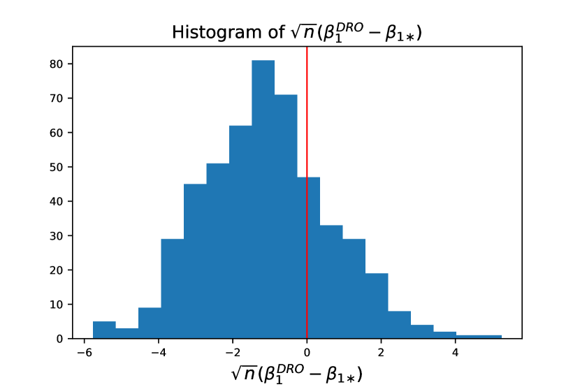
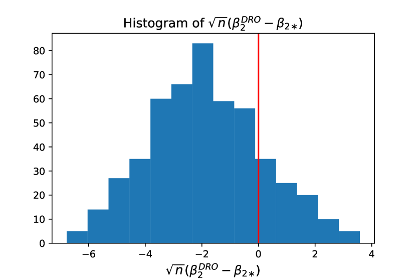
Figure 1: Histogram of $\beta_{n}^{DRO}$

4 Proposed Adjusted WDRO Estimator

This section introduces the formal formulation of our adjusted WDRO estimator and investigates the relevant properties, e.g., unbiasedness.

The adjusted WDRO estimator is based on the asymptotic distribution obtained in Section 3.2 and the adjustment technique introduced in Section 2. Recall the WDRO estimator has the following convergence:

$$\sqrt{n}(\beta_{n}^{\text{DRO}}-\beta_{\ast})\Rightarrow\mathcal{N}\left(-C(\beta_{\ast})^{-1}H\left(\beta_{\ast}\right),D\right),$$

where

$$C(\beta_{\ast})=\mathbb{E}_{P_{\ast}}\left[\frac{\partial^{2}L(f(\mathbf{X},\beta),Y)}{\partial\beta^{2}}\right]\Bigg{|}_{\beta=\beta_{\ast}},\quad H(\beta_{\ast})=\tau\frac{\partial\sqrt{\mathbb{E}_{P_{\ast}}\left[\left\|\frac{\partial L(f(\mathbf{X},\beta),Y)}{\partial\mathbf{X}}\right\|_{2}^{2}\right]}}{\partial\beta}\Bigg{|}_{\beta=\beta_{\ast}}.$$

Notice that the asymptotic bias $f(\beta_{\ast})=-C(\beta_{\ast})^{-1}H\left(\beta_{\ast}\right)$ depends on the underlying distribution $P_{\ast}$, then we use the associated empirical distribution to approximate $f$. Applying the adjusted technique proposed in Theorem 3, we define the adjusted WDRO estimator in the following.

Definition 12 (Adjusted WDRO Estimator)

In the WDRO problem (4), under Assumption 5, 7, and 8, the adjusted WDRO estimator is defined by

$$\beta_{n}^{ADRO}=\mathcal{A}_{n}(\beta_{n}^{DRO}),$$ (10)

where

$$\mathcal{A}_{n}(\mathbf{z})=\mathbf{z}+\frac{C_{n}(\mathbf{z})^{-1}H_{n}(\mathbf{z})}{\sqrt{n}},$$

$$H_{n}(\mathbf{z})=\tau\frac{\partial\sqrt{\mathbb{E}_{\mathbb{P}_{n}}\left[\left\|\frac{\partial L(f(\mathbf{X},\beta),Y)}{\partial\mathbf{X}}\right\|_{2}^{2}\right]}}{\partial\beta}\Bigg{|}_{\beta=\mathbf{z}},$$ (11)

$$C_{n}(\mathbf{z})=\mathbb{E}_{\mathbb{P}_{n}}\left[\frac{\partial^{2}L(f(\mathbf{X},\beta),Y)}{\partial\beta^{2}}\right]\Bigg{|}_{\beta=\mathbf{z}}.$$ (12)

To promise the existence of the adjusted WDRO estimator, we need additional conditions to let the matrix $C_{n}(\beta_{n}^{DRO})$ be invertible and the vector $H_{n}(\beta_{n}^{DRO})$ well-defined. The conditions are shown in the following proposition.

Proposition 13 (Existence of Adjusted WDRO Estimator I)

For the empirical distribution $\mathbb{P}_{n}$, the loss function $L(f(\mathbf{x},\beta),y)$ and the WDRO estimator $\beta_{n}^{DRO}$, if

$$\mathbb{P}_{n}\left(\left\|\frac{\partial L(f(\mathbf{X},\beta),Y)}{\partial\mathbf{X}}\right\|_{2}^{2}\Bigg{|}_{\beta=\beta_{n}^{DRO}}\not=0\right)>0,\quad\mathbb{E}_{\mathbb{P}_{n}}\left[\frac{\partial^{2}L(f(\mathbf{X},\beta),Y)}{\partial\beta^{2}}\right]\Bigg{|}_{\beta=\beta_{n}^{DRO}}\succ 0$$

hold, then the adjusted WDRO estimator $\beta_{n}^{ADRO}$ defined in (10) exists.

If the hypothesis function is linear, i.e., $f=\langle\mathbf{x},\beta\rangle$, the existence conditions demonstrated in Proposition 13 could be further simplified as shown in the following proposition.

Proposition 14 (Existence of Adjusted WDRO Estimator II)

For the empirical distribution $\mathbb{P}_{n}$, the loss function $L(\langle\mathbf{x},\beta\rangle,y)$ and the WDRO estimator $\beta_{n}^{DRO}$, if

$$\beta_{n}^{DRO}\not=0,\quad\frac{\partial^{2}L(f,y)}{\partial f^{2}}\not=0,\quad\mathbb{P}_{n}\left(\frac{\partial L(\langle\mathbf{X},\beta_{n}^{DRO}\rangle,Y)}{\partial f}\not=0\right)>0,$$

hold, and there does not exist nonzero vector $\alpha$ such that $\mathbb{P}_{n}(\alpha^{\top}\mathbf{X}=0)=1$, then the adjusted WDRO estimator $\beta_{n}^{ADRO}$ defined in (10) exists.

The conditions in Proposition 13 and 14 are mild. For example, for the nonzero WDRO estimator $\beta_{n}^{DRO}$ and non-degenerate loss $L$, if the distribution of feature variable $\mathbf{X}$ does not concentrate, the conditions in Proposition 14 can hold without loss of generality. One may check that the existence conditions could be satisfied by multiple statistical models, including linear regression, and logistic regression, among many others.

4.1 Simplication of the Adjusted WDRO Estimator

We discuss under which conditions the expression of the adjusted WDRO estimator $\beta_{n}^{ADRO}$ could be further simplified in this subsection.

Recall that, in the definition of the adjusted WDRO estimator (Definition 12), the term $H(\cdot)$ appears complicated at first glance. The following proposition shows that the function $H(\cdot)$ can be simplified under certain conditions.

Proposition 15

If the hypothesis function in problem (4) is a linear function, i.e., $f(\mathbf{x},\beta)=\langle\mathbf{x},\beta\rangle$, and the equation

$$\mathbb{E}_{P_{\ast}}\left[\frac{\partial L(f(\mathbf{X},\beta_{\ast}),Y)}{\partial f}\frac{\partial L^{2}(f(\mathbf{X},\beta_{\ast}),Y)}{\partial f^{2}}\mathbf{X}\right]=0,$$ (13)

where $\frac{\partial L}{\partial f}$ means taking the gradient of $L(\cdot,\cdot)$ w.r.t. the first argument, holds for the underlying data-generating distribution $P_{\ast}$ and the loss function $L(\cdot,\cdot)$, then the function $H(\beta_{\ast})$ defined in (8) can be rewritten as

$$H(\beta_{\ast})=\tau\frac{\beta_{\ast}}{{\|\beta_{\ast}\|_{2}}}\sqrt{\mathbb{E}_{P_{\ast}}\left[\left(\frac{\partial L(f(\mathbf{X},\beta),Y)}{\partial f}\right)^{2}\right]}\Bigg{|}_{\beta=\beta_{\ast}}.$$

Proposition 15 implies that the linearity of the hypothesis function and the equation (13) can promise $H(\beta_{\ast})$ could be written as a rescaling of $\beta_{\ast}$. The associated function $H_{n}(\mathbf{z})$ is defined by

$$H_{n}(\mathbf{z})=\tau\frac{\beta_{\ast}}{{\|\beta_{\ast}\|_{2}}}\sqrt{\mathbb{E}_{\mathbb{P}_{n}}\left[\left(\frac{\partial L(f(\mathbf{X},\beta),Y)}{\partial f}\right)^{2}\right]}\Bigg{|}_{\beta=\mathbf{z}}.$$

In this way, the expression of the adjusted WDRO estimator could be simplified. In particular, the conditions in Proposition 15 can be satisfied by multiple statistical models, e.g., linear regression, logistic regression, and Poisson regression. The details can be found in Section 5.

4.2 Asymptotically Unbiased

We establish the asymptotic distribution of the adjusted WDRO estimator $\beta_{n}^{ADRO}$.

Theorem 16

Under Assumption 5, 7, and 8, if the adjusted WDRO estimator $\beta_{n}^{ADRO}$ defined in (10) exists, $\frac{\partial L(f(\mathbf{x},\beta),y)}{\partial x\partial\beta}$ and $\frac{\partial^{2}L(f(\mathbf{x},\beta),y)}{\partial\beta^{2}}$ are continuously differentiable w.r.t $\beta$ at some neighborhood of $\beta_{\ast}$, and the gradient of $C_{n}(\mathbf{z})^{-1}H_{n}(\mathbf{z})$ at $\beta_{\ast}$ is bounded in probability, then $\beta_{n}^{ADRO}$ converges in distribution:

$$\sqrt{n}(\beta_{n}^{ADRO}-\beta_{\ast})\Rightarrow\mathcal{N}(0,D),$$

where $D$ is defined in (9).

Theorem 16 indicates that our proposed estimator $\beta^{ADRO}_{n}$ is asymptotically unbiased and the asymptotic mean squared error is $\mathrm{tr}(D)$. Recall the asymptotic distribution of the classic WDRO estimator $\beta_{n}^{DRO}$ is

$$\sqrt{n}(\beta_{n}^{\text{DRO}}-\beta_{\ast})\Rightarrow\mathcal{N}\left(-C(\beta_{\ast})^{-1}H\left(\beta_{\ast}\right),D\right),$$

indicating that the asymptotic mean squared error of the classic WDRO estimator $\beta_{n}^{DRO}$ is $\mathrm{tr}(D)+f(\beta_{\ast})^{\top}f(\beta_{\ast})$, where $f(\beta_{\ast})=-C(\beta_{\ast})^{-1}H(\beta_{\ast})$. In this way, our proposed estimator has a smaller asymptotic mean squared error.

4.3 Out-of-sample Performance Guarantee

This subsection discusses the out-of-sample performance guarantee for the adjusted WDRO estimator $\beta_{n}^{ADRO}$.

Informally, the out-of-sample performance guarantee for the WDRO estimator $\beta_{n}^{DRO}$ reads that, with high probability, the following inequality holds,

$$\mathbb{E}_{P_{\ast}}\left[L(f(\mathbf{X},\beta_{n}^{DRO}),Y)\right]\leq\sup_{P\in\mathcal{U}_{\rho_{n}}(\mathbb{P}_{n})}\mathbb{E}_{P}\left[L(f(\mathbf{X},\beta_{n}^{DRO}),Y)\right]+\epsilon_{n},$$ (14)

where the left-hand side is the generalization error of $\beta_{n}^{DRO}$, and the first term on the right-hand side is called Wasserstein robust loss of $\beta_{n}^{DRO}$. Inequality (14) implies that the ground-truth error of $\beta_{n}^{DRO}$ is upper bounded by the Wasserstein robust loss up to a higher order residual $\epsilon_{n}$.

Recall that our proposed adjusted estimator $\beta_{n}^{ADRO}$ is transformed from the WDRO estimator $\beta_{n}^{DRO}$. As the WDRO estimator $\beta_{n}^{DRO}$ enjoys the out-of-sample performance guarantee (14), similar arguments can be established towards the adjusted WDRO estimator $\beta_{n}^{ADRO}$.

Corollary 17 (Performance Guarantee)

Suppose the generalization bound (14) holds for the WDRO estimator $\beta_{n}^{DRO}$ for some residual term $\epsilon_{n}$ with probability $1-\alpha$. If the loss function $L(f(\mathbf{x},\beta),y)$ is $h$-Lipschitz continuous w.r.t. $\beta$ and the adjusted WDRO estimator $\beta_{n}^{ADRO}$ exists, then the following inequality,

$$\mathbb{E}_{P_{\ast}}\left[L(f(\mathbf{X},\beta_{n}^{ADRO}),Y)\right]\leq\sup_{P\in\mathcal{U}_{\rho_{n}}(\mathbb{P}_{n})}\mathbb{E}_{P}\left[L(f(\mathbf{X},\beta_{n}^{ADRO}),Y)\right]+2h\|\beta_{n}^{DRO}-\beta_{n}^{ADRO}\|_{2}+\epsilon_{n},$$

holds with probability $1-\alpha$.

From the definition of the adjusted WDRO estimator $\beta_{n}^{ADRO}$, we know that the term $\|\beta_{n}^{DRO}-\beta_{n}^{ADRO}\|_{2}$ is of order $\mathcal{O}(1/\sqrt{n})$. In addition, Gao (2022) derives the generalization bound based on a novel variance-based concentration inequality for the empirical loss for the radius of the order $\mathcal{O}(1/\sqrt{n})$, where $\epsilon_{n}=\widetilde{\mathcal{O}}(1/n)$. In this sense, the generalization error of the adjusted WDRO estimator $\beta_{n}^{ADRO}$ can be upper bounded by the Wasserstein robust loss of the adjusted WDRO estimator $\beta_{n}^{ADRO}$ up to a new residual term, $2h\|\beta_{n}^{DRO}-\beta_{n}^{ADRO}\|_{2}+\epsilon_{n}$, which is of order $\mathcal{O}(1/\sqrt{n})$.

The discussions above demonstrate that an upper confidence bound can be derived on the out-of-sample error of our proposed estimator $\beta_{n}^{ADRO}$. As a result, the adjustment strategy won’t sacrifice the WDRO estimator’s capacity for generalization.

5 Adjusted WDRO in the Generalized Linear Model

The generalized linear model is considered in this section since several well-known regression models can be covered, including logistic regression, Poisson regression, and linear regression. We introduce how to develop the associated adjusted WDRO estimators.

5.1 Formulation of the Generalized Linear Model

In the generalized linear model, the label variable $Y$ is generated from a particular distribution from the exponential family, including the Bernoulli distribution on $Y\in\{-1,1\}$ in the logistic regression, the Poisson distribution on $Y\in\{0,1,2,...\}$ in the Poisson regression, the normal distribution on $Y\in\mathbb{R}$ in the linear regression, etc. The expectation of the label variable $Y$ conditional on the feature variable $\mathbf{X}$ is determined by the link function. With a little abuse of notation, if we denote the nonzero ground-truth parameter by $\beta_{\ast}$ and the link function by $G(\cdot)$, we have $G(\mathbb{E}[Y|\mathbf{X}=\mathbf{x}])=\langle\mathbf{x},\beta_{\ast}\rangle$, where the link functions $G(\cdot)$ are chosen as the logit function in the logistic regression, the log function in the Poisson regression, the identity function in the linear regression, etc. If we denote the logit function, the log function, and the identity function by $G^{1}(\cdot)$, $G^{2}(\cdot)$, and $G^{3}(\cdot)$, respectively, we have

$$G^{1}(t)=\log\left(\frac{t}{1-t}\right),\quad G^{2}(t)=e^{t},\quad G^{3}(t)=t.$$

In the generalized linear model, the ground-truth parameter $\beta_{\ast}$ is estimated by the maximum likelihood estimation method, and the associated loss function can be denoted by $L(f(\mathbf{x},\beta),y)=L(\langle\mathbf{x},\beta\rangle,y)$. If we denote the loss function in the logistic regression, the Poisson regression and the linear regression by $L^{1}(\cdot,\cdot)$, $L^{2}(\cdot,\cdot)$, and $L^{3}(\cdot,\cdot)$, respectively, we have

$$L^{1}\left(\langle\mathbf{x},\beta\rangle,y\right)=\log(1+e^{-y\langle\mathbf{x},\beta\rangle}),$$

$$L^{2}\left(\langle\mathbf{x},\beta\rangle,y\right)=e^{\langle\mathbf{x},\beta\rangle}-y\langle\mathbf{x},\beta\rangle,$$

$$L^{3}(\langle\mathbf{x},\beta\rangle,y)=\frac{1}{2}\left(\langle\mathbf{x},\beta\rangle-y\right)^{2},$$

where $\beta\in B$, $B$ is a compact convex subset of $\mathbb{R}^{d}$, $\beta_{\ast}\in{B}^{\circ}$, and $\mathbf{x}\in\Omega\subset\mathbb{R}^{d}$.

5.2 Asymptotic Convergence of the WDRO Estimator

This subsection derives the convergence of the WDRO estimator $\beta^{DRO}_{n}$ in the linear regression, logistic regression, and Poisson regression.

Suppose that our choice of hyperparameters follows Assumption 5. As demonstrated in Section 3.2, we check Assumption 7 and Assumption 8 in the following lemmas.

Lemma 18

The loss function $L^{1}(\langle\mathbf{x},\beta\rangle,y)$ satisfies the conditions in Assumption 7.

Lemma 19

If $\Omega$ is bounded, the loss function $L^{2}(\langle\mathbf{x},\beta\rangle,y)$ satisfies the conditions Assumption 7.

Lemma 20

The loss function $L^{3}(\langle\mathbf{x},\beta\rangle,y)$ satisfies the conditions Assumption 7.

Lemma 21

In the logistic regression, if there does not exist nonzero vector $\alpha$ such that $P_{\ast}(\alpha^{\top}\mathbf{X}=0)=1$, and $\mathbb{E}_{P_{\ast}}\left[\|\mathbf{X}\|_{2}^{2}\right]<\infty$, Assumption 8 is satisfied.

Lemma 22

In the Poisson regression, if there does not exist nonzero vector $\alpha$ such that $P_{\ast}(\alpha^{\top}\mathbf{X}=0)=1$, and $\mathbb{E}_{P_{\ast}}[\|\mathbf{X}\|_{2}^{2}e^{\langle\mathbf{X},\beta_{\ast}\rangle}]<\infty$, Assumption 8 is satisfied.

Lemma 23

In the linear regression, if there does not exist nonzero vector $\alpha$ such that $P_{\ast}(\alpha^{\top}\mathbf{X}=0)=1$, and $\mathbb{E}_{P_{\ast}}[\|\mathbf{X}\|_{2}^{2}]<\infty$, Assumption 8 is satisfied.

Lemma 18-20 imply that the loss functions satisfy the conditions in Assumption 7 while Lemma 21-23 show that Assumption 8 can be simplified in the logistic regression, Poisson regression, and linear regression.

Equipped with Lemma 18-23, the convergence in distribution of the WDRO estimator $\beta_{n}^{DRO}$ can be established due to Theorem 9. The following three propositions give the explicit expression of the asymptotic distribution of the WDRO estimator for the logistic regression, Poisson regression, and linear regression.

Proposition 24 (Convergence of $\beta_{n}^{DRO}$ in the logistic regression)

In the logistic regression, under Assumption 5, if $\Omega=\mathbb{R}^{d}$ and $\mathbb{E}\left[\|\mathbf{X}\|_{2}^{2}\right]<\infty$, and there does not exist nonzero vector $\alpha$ such that $P_{\ast}(\alpha^{\top}\mathbf{X}=0)=1$, the WDRO estimator $\beta_{n}^{DRO}$ converges in distribution:

$$\sqrt{n}(\beta_{n}^{DRO}-\beta_{\ast})\Rightarrow\mathcal{N}(-C(\beta_{\ast})^{-1}H(\beta_{\ast}),D),$$

where

$$D=\left(\mathbb{E}_{P_{\ast}}\left[\frac{\mathbf{X}\mathbf{X}^{\top}}{\left(1+e^{Y\langle\mathbf{X},\beta_{\ast}\rangle}\right)^{2}}\right]\right)^{-1},$$ (15)

and

$$C(\beta_{\ast})=\mathbb{E}_{P_{\ast}}\left[\frac{\mathbf{X}\mathbf{X}^{\top}e^{\langle\mathbf{X},\beta_{\ast}\rangle}}{\left(1+e^{\langle\mathbf{X},\beta_{\ast}\rangle}\right)^{2}}\right],\quad H(\beta_{\ast})=\tau\frac{\beta_{\ast}}{\|\beta_{\ast}\|_{2}}\sqrt{\mathbb{E}_{P_{\ast}}\left[\frac{e^{\langle\mathbf{X},\beta_{\ast}\rangle}}{\left(1+e^{\langle\mathbf{X},\beta_{\ast}\rangle}\right)^{2}}\right]}.$$ (16)

Proposition 25 (Convergence of $\beta_{n}^{DRO}$ in the Poisson regression)

In the Poission regression, under Assumption 5, if $\Omega$ is compact and can be expressed as $\Omega=\{\mathbf{x}\in\mathbb{R}^{d}:A\mathbf{x}\leq b\}$, where $A$ is an $l\times d$ matrix with linearly independent rows and $b\in\mathbb{R}^{l}$, $\mathbb{E}_{P_{\ast}}[\|\mathbf{X}\|_{2}^{3}e^{\langle\mathbf{X},\beta_{\ast}\rangle}]<\infty$, there does not exist nonzero vector $\alpha$ such that $P_{\ast}(\alpha^{\top}\mathbf{X}=0)=1$, and $\mathbf{X}$ has a probability density which is absolutely continuous w.r.t. Lebesgue measure, the WDRO estimator $\beta_{n}^{DRO}$ converges in distribution:

$$\sqrt{n}(\beta_{n}^{DRO}-\beta_{\ast})\Rightarrow\mathcal{N}(-C(\beta_{\ast})^{-1}H(\beta_{\ast}),D),$$

where

$$D=\left(\mathbb{E}_{P_{\ast}}\left[\mathbf{X}\mathbf{X}^{\top}e^{\langle\mathbf{X},\beta_{\ast}\rangle}\right]\right)^{-1},$$ (17)

and

$$C(\beta_{\ast})=\mathbb{E}_{P_{\ast}}\left[\mathbf{X}\mathbf{X}^{\top}e^{\langle\mathbf{X},\beta_{\ast}\rangle}\right],\quad H(\beta_{\ast})=\tau\frac{\beta_{\ast}}{\|\beta_{\ast}\|_{2}}\sqrt{\mathbb{E}_{P_{\ast}}[e^{\langle\mathbf{X},\beta_{\ast}\rangle}]}.$$ (18)

Proposition 26 (Convergence of $\beta_{n}^{DRO}$ in the linear regression)

In the linear regression, under Assumption 5, if $\Omega=\mathbb{R}^{d}$, and $\mathbb{E}_{P_{\ast}}[\|\mathbf{X}\|_{2}^{2}]<\infty$, and there does not exist nonzero vector $\alpha$ such that $P_{\ast}(\alpha^{\top}\mathbf{X}=0)=1$, the WDRO estimator $\beta_{n}^{DRO}$ converges in distribution:

$$\sqrt{n}(\beta_{n}^{DRO}-\beta_{\ast})\Rightarrow\mathcal{N}(-C^{-1}H(\beta_{\ast}),D),$$

where

$$D=\sigma^{2}\left(\mathbb{E}_{P_{\ast}}\left[\mathbf{X}\mathbf{X}^{\top}\right]\right)^{-1},$$ (19)

$$C=\mathbb{E}_{P_{\ast}}\left[\mathbf{X}\mathbf{X}^{\top}\right],\quad H(\beta_{\ast})=\tau\sigma\frac{\beta_{\ast}}{\|\beta_{\ast}\|_{2}},$$ (20)

and $\mathrm{Var}(Y|\mathbf{X})=\sigma^{2},\sigma>0$

We could obtain the associated adjusted WDRO estimators based on the convergence results derived in Proposition 24-26, and the details will be clarified in the next subsection.

Also, the proofs of Proposition 24-26 are relegated to Appendix A. The proofs show that the conditions in Proposition 15 are satisfied, which enables us to simplify the function $H(\cdot)$, seeing (16), (18) and (20).

5.3 Adjusted WDRO Estimator in the Generalized Linear Model

This subsection gives the formulations of the adjusted WDRO estimator for logistic regression, Poisson regression, and linear regression by plugging the expressions of the function $C(\cdot)$ and $H(\cdot)$ in (16), (18) and (20) into the definition of the adjusted WDRO estimator (10).

Definition 27

Under assumptions in Proposition 24-26, for the nonzero WDRO estimator $\beta_{n}^{DRO}$, we define the adjusted WDRO estimator $\beta_{n}^{ADRO}$ as follows,

$$\beta_{n}^{ADRO}=\beta_{n}^{DRO}+\frac{\tau}{\sqrt{n}}\sqrt{\mathbb{E}_{\mathbb{P}_{n}}\left[\frac{e^{\langle\mathbf{X},\beta_{n}^{DRO}\rangle}}{\left(1+e^{\langle\mathbf{X},\beta_{n}^{DRO}\rangle}\right)^{2}}\right]}\left(\mathbb{E}_{\mathbb{P}_{n}}\left[\frac{\mathbf{X}\mathbf{X}^{\top}e^{\langle\mathbf{X},\beta_{n}^{DRO}\rangle}}{\left(1+e^{\langle\mathbf{X},\beta_{n}^{DRO}\rangle}\right)^{2}}\right]\right)^{-1}\frac{\beta_{n}^{DRO}}{\|\beta_{n}^{DRO}\|_{2}},$$ (21)

$$\beta_{n}^{ADRO}=\beta_{n}^{DRO}+\frac{\tau}{\sqrt{n}}\sqrt{\mathbb{E}_{\mathbb{P}_{n}}[e^{\langle\mathbf{X},\beta_{n}^{DRO}\rangle}]}\left(\mathbb{E}_{\mathbb{P}_{n}}\left[\mathbf{X}\mathbf{X}^{\top}e^{\langle\mathbf{X},\beta_{n}^{DRO}\rangle}\right]\right)^{-1}\frac{\beta_{n}^{DRO}}{\|\beta_{n}^{DRO}\|_{2}},$$

$$\beta_{n}^{ADRO}=\beta_{n}^{DRO}+\frac{\tau\sigma}{\sqrt{n}}\left(\mathbb{E}_{\mathbb{P}_{n}}\left[\mathbf{X}\mathbf{X}^{\top}\right]\right)^{-1}\frac{\beta_{n}^{DRO}}{\|\beta_{n}^{DRO}\|_{2}},$$ (22)

for the logistic regression, Poisson regression, and linear regression, respectively.

Without loss of generality, as we discussed in Proposition 14, the adjusted WDRO estimators defined in Definition 27 are well-defined. Then, we check the conditions in Theorem 16 hold in the following theorem to show that the proposed adjustment technique could de-bias the associated adjusted WDRO estimators successfully in the logistic regression, Poisson regression, and linear regression.

Theorem 28

For the adjusted WDRO estimator $\beta_{n}^{ADRO}$ defined in Definition 27, we have the following

$$\sqrt{n}\left(\beta_{n}^{ADRO}-\beta_{\ast}\right)\Rightarrow\mathcal{N}(0,D),$$

where $D$ is defined by (15), (17), and (19) in the logistic regression, Poisson regression, and linear regression, respectively.

6 Numerical Experiments

In this section, we investigate the empirical performance of the adjusted WDRO estimator $\beta_{n}^{ADRO}$, compared with the classic WDRO estimator $\beta_{n}^{DRO}$.

6.1 Experiment Setting

The WDRO algorithmic framework of the logistic regression model and linear regression model with quadratic loss has been established in Blanchet et al. (2022c). Therefore, the adjusted estimators in the logistic regression model and the linear regression model are implemented as examples to help explore the practical performance of our adjusting technique.

6.1.1 Logistic Regression

Assume the feature variable $\mathbf{X}$ follows the multivariate standard normal distribution. Suppose $\mathbf{X}$ follows 2-dimensional standard normal distribution, and the label variable $Y$ follows the Bernoulli distribution, where $\mathbb{P}(Y=1|\mathbf{X}=\mathbf{x})=1/(1+e^{-\langle\mathbf{x},\beta_{\ast}\rangle})$ and $\beta_{\ast}=(1/\sqrt{17},4/\sqrt{17})$. Data is generated $5$ times for each sample size $n\in\{500,700,1000,1500,$ $1800,2000\}$. The WDRO estimator $\beta_{n}^{DRO}$ is computed by the iterative algorithm in Blanchet et al. (2022c). The adjusted WDRO estimator $\beta_{n}^{ADRO}$ is computed via equation (21). Per the iterative algorithm, we set the learning rate as $0.3$ and the maximum number of iterations as $50000$, respectively. Moreover, the value of $\tau$, which is the coefficient in the Wasserstein radius $\rho_{n}=\tau/\sqrt{n}$, should be determined, so we let $\tau\in\{1.5,2,2.5,3\}$.

6.1.2 Linear regression

Assume the feature variable $\mathbf{X}$ follows the 2-dimensional standard normal distribution, and the label variable $Y$ follows normal distribution, where $Y|\mathbf{X}=\mathbf{x}\sim\mathcal{N}(\langle\mathbf{x},\beta_{\ast}\rangle,\sigma)$, $\beta_{\ast}=(3/\sqrt{10},-1/\sqrt{10})$. We set $\sigma=0.1$. Data is generated $5$ times for each sample size $n\in\{500,700,1000,1500,1800,2000\}$. The WDRO estimator $\beta_{n}^{DRO}$ is computed by the iterative algorithm in Blanchet et al. (2022c). The adjusted WDRO estimator $\beta_{n}^{ADRO}$ is computed via equation (22). Per the iterative algorithm, we set the learning rate as $0.05$ and the maximum number of iterations as $50000$, respectively. Then, we set the value of $\tau$ as $\tau\in\{1.5,2,2.5,3\}$.

6.2 Experiment Results

The experimental results of the logistic regression are reported in Figure 2-5, and the results of the linear regression are reported in Figure 6-9.

The performance of the estimators is evaluated by the squared error. The squared error is defined by $\|\widehat{\beta}-\beta_{\ast}\|_{2}^{2}$, where $\widehat{\beta}$ denotes the associated estimator. We plot the mean squared error of $\beta_{n}^{DRO}$ and $\beta_{n}^{ADRO}$ versus the logarithm of the sample size $n$, respectively. From the figures, we observe that the line of mean squared error of $\beta_{n}^{DRO}$ is always above that of $\beta_{n}^{ADRO}$, illustrating that the proposed adjusted estimator has a smaller mean squared error in empirical experiments. Recall that the adjusted WDRO estimator has a better asymptotic mean squared error in theory, while our empirical results show that our estimator also outperforms even when the sample size is finite. Moreover, we compute the difference of the squared error between $\beta_{n}^{DRO}$ and $\beta_{n}^{ADRO}$ for each case. This quantity can help us to evaluate the improvement achieved by the adjustment technique for each run. To visualize the improvement, we plot the boxplots for each sample size and each value of $\tau$. The figures show that most parts of the boxplots are located above $y=0$ in the logistic regression, and all of the boxplots are located above $y=0$ in the linear regression. These observations indicate that the adjustment technique can generate a more accurate estimator of the ground-truth parameter $\beta_{\ast}$.

In addition to the squared error, we investigate the empirical loss (i.e., the log-likelihood) of the linear regression and the logistic regression. Similar to how we analyze the squared loss, we plot the mean loss and the case-wise loss improvement. The figures show that the adjustment technique could reduce the empirical loss.

Overall, the adjusted WDRO estimator has better empirical performance than the classic WDRO estimator. When people plan to estimate parameters in the statistical learning model, the proposed adjusted estimator can be considered.

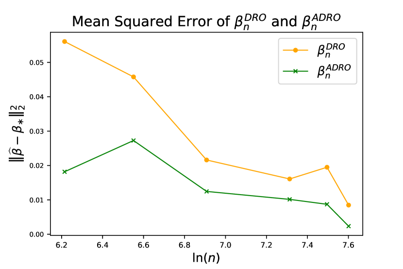
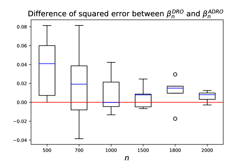
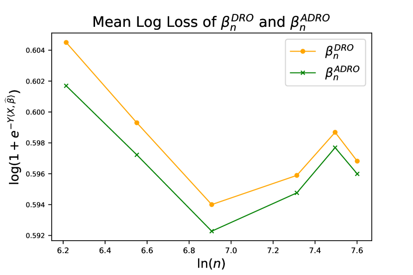
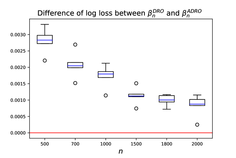
Figure 2: Squared error and log loss plots of the logistic regression, $\tau=1.5$.

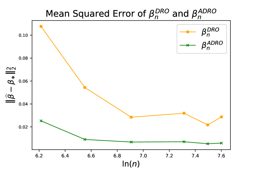
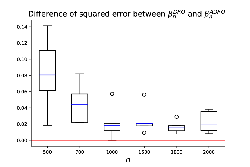
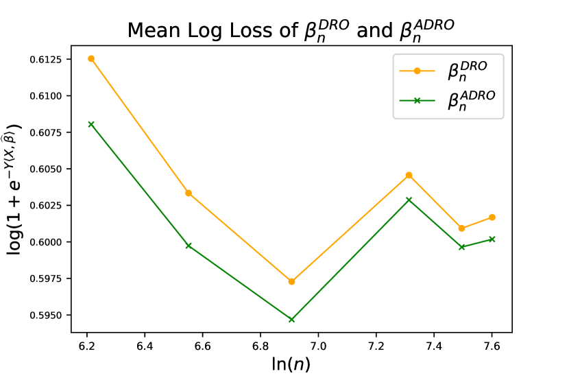
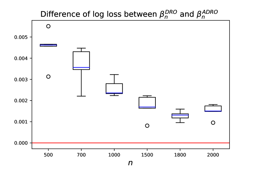
Figure 3: Squared error and log loss plots of the logistic regression, $\tau=2$.

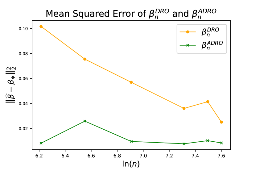
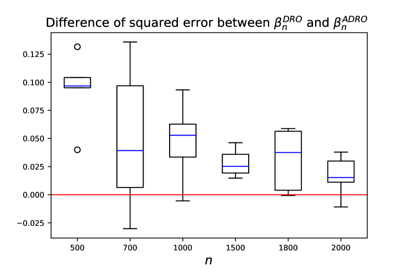
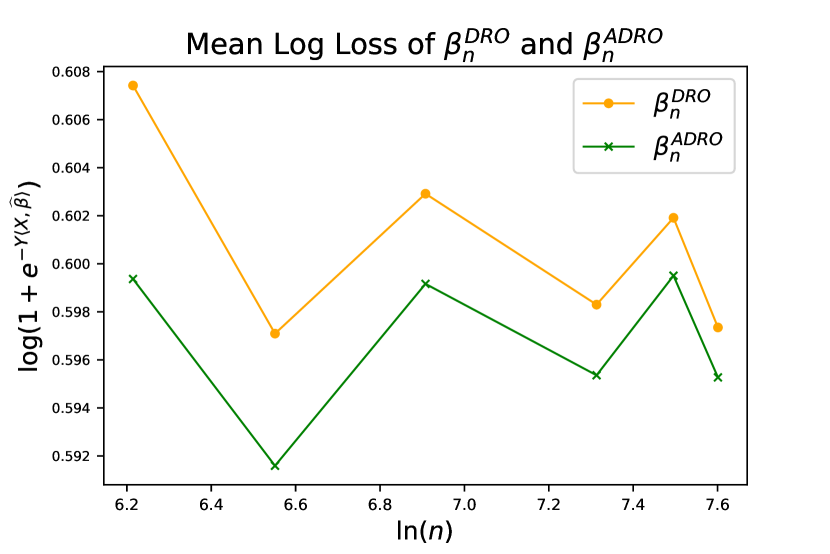
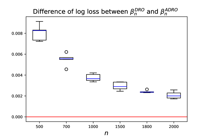
Figure 4: Squared error and log loss plots of the logistic regression, $\tau=2.5$.

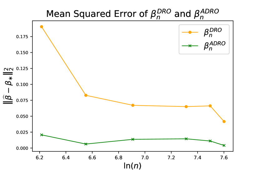
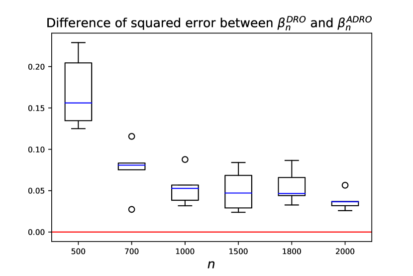
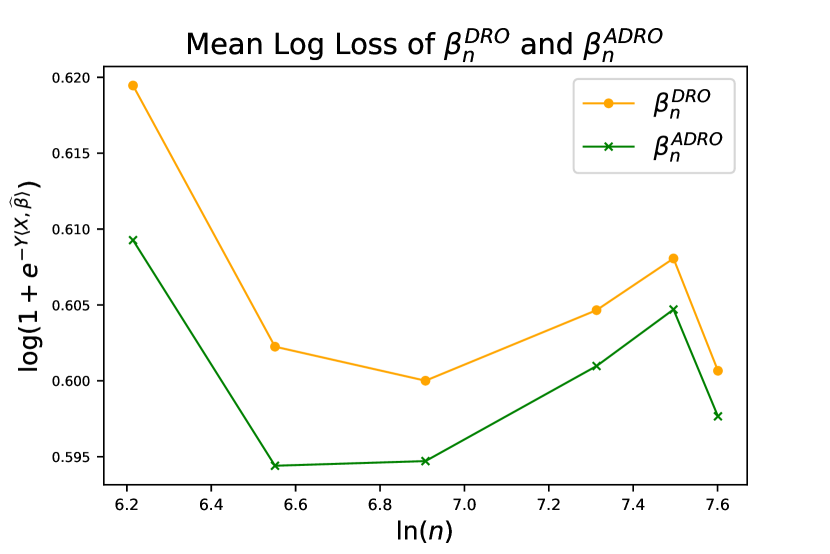
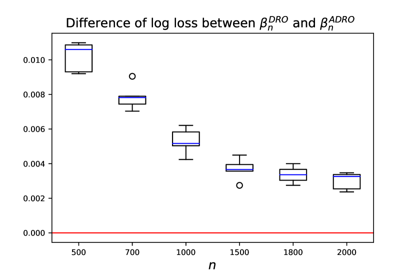
Figure 5: Squared error and log loss plots of the logistic regression, $\tau=3$.

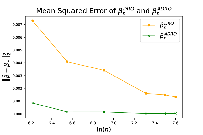
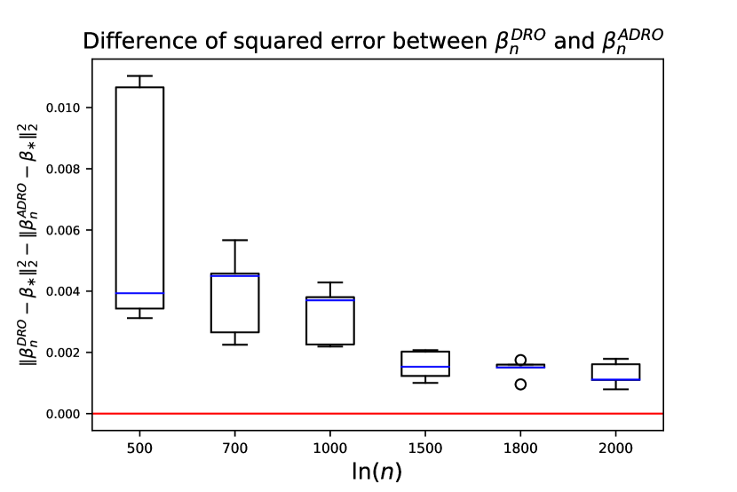
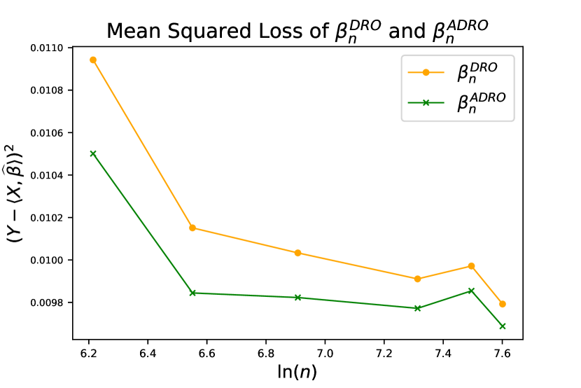
Figure 6: Squared error and squared loss plots of the linear regression, $\tau=1.5$.

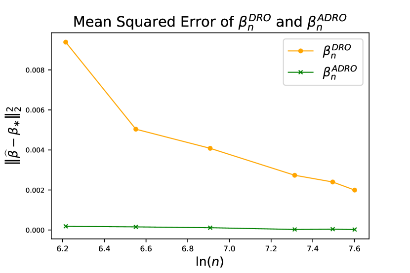
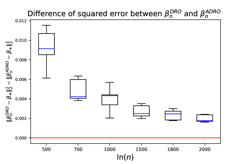
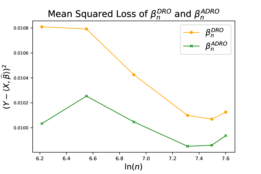
Figure 7: Squared error and squared loss plots of the linear regression, $\tau=2$.

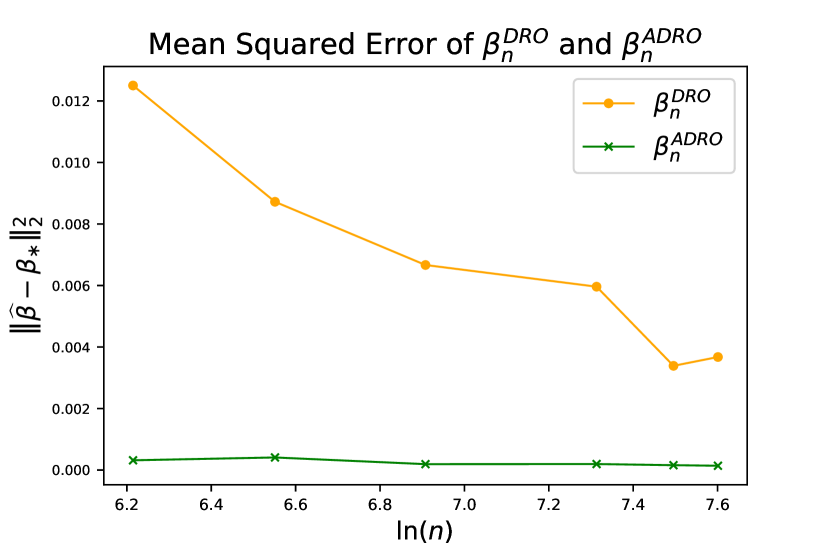
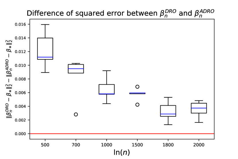
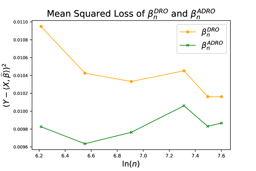
Figure 8: Squared error and squared loss plots of the linear regression, $\tau=2.5$.

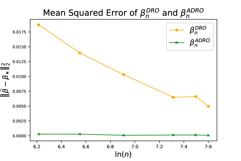
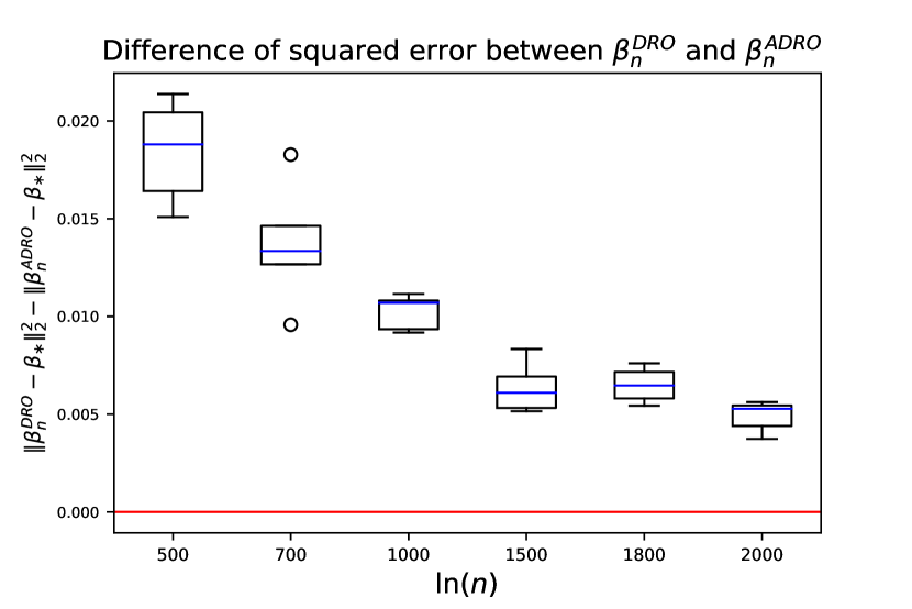
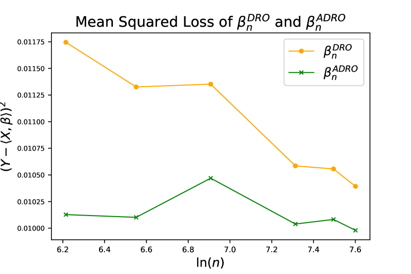
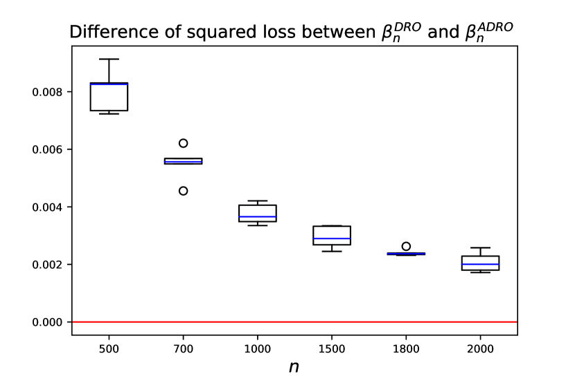
Figure 9: Squared error and squared loss plots of the linear regression, $\tau=3$.

7 Discussion

This paper improves the performance of the WDRO estimator through the lens of the statistical asymptotic behavior in statistical learning. To the best of our knowledge, we are the first to propose transformations to de-bias the WDRO estimator. The proposed adjusted WDRO estimator is asymptotically unbiased with a smaller asymptotic mean squared error. Also, the adjusted WDRO estimator is easy to compute as long as the classic WDRO estimator is known.

Notably, in the development of our theory and methodology, we also carefully clarify and check the corresponding assumptions, providing a rigorous scheme to apply and generalize our adjustment technique.

Acknowledgments and Disclosure of Funding

This project is partially supported by the Transdisciplinary Research Institute for Advancing Data Science (TRIAD), https://research.gatech.edu/data/triad, which is a part of the TRIPODS program at NSF and located at Georgia Tech, enabled by the NSF grant CCF-1740776. The authors are also partially sponsored by NSF grants 2015363.

Appendix A Proof

A.1 Proof of Proposition 1

Proof  Due to the sequential delta method (Theorem 4), we have that

$$\sqrt{n}\left(\phi_{n}(\beta_{n})-\phi_{n}(\beta_{\ast})\right)\Rightarrow\mathcal{N}(\phi^{\prime}(\beta_{\ast})f(\beta_{\ast}),\phi^{\prime}(\beta_{\ast})D\phi^{\prime}(\beta_{\ast})^{\top}),$$

which is equivalent to

$$\sqrt{n}\left(\phi_{n}(\beta_{n})-\beta_{\ast}\right)+\sqrt{n}\left(\beta_{\ast}-\phi_{n}(\beta_{\ast})\right)\Rightarrow\mathcal{N}(\phi^{\prime}(\beta_{\ast})f(\beta_{\ast}),\phi^{\prime}(\beta_{\ast})D\phi^{\prime}(\beta_{\ast})^{\top}).$$

To make the distribution of $\sqrt{n}\left(\phi_{n}(\beta_{n})-\beta_{\ast}\right)$ have a finite limit, we should require the following holds

$$\beta_{\ast}-\phi_{n}(\beta_{\ast})=\mathcal{O}\left(\frac{1}{\sqrt{n}}\right),$$

which is equivalent to

$$\phi_{n}(\beta_{\ast})=\beta_{\ast}+\mathcal{O}\left(\frac{1}{\sqrt{n}}\right),$$

indicating

$$\phi_{n}^{\prime}(\beta_{\ast})\to I.$$

In this way, we have that

$$\sqrt{n}\left(\phi_{n}(\beta_{n})-\beta_{\ast}\right)+\sqrt{n}\left(\beta_{\ast}-\phi_{n}(\beta_{\ast})\right)\Rightarrow\mathcal{N}(f(\beta_{\ast}),D).$$

Without loss of generality, we assume that

$$\phi_{n}(\beta_{\ast})=\beta_{\ast}-\frac{1}{\sqrt{n}}g(\beta_{\ast})+o\left(\frac{1}{\sqrt{n}}\right),$$

then we could have that

$$\sqrt{n}\left(\phi_{n}(\beta_{n})-\beta_{\ast}\right)\sim\mathcal{N}\left(f(\beta_{\ast})-g(\beta_{\ast}),D\right).$$

Consequently, the least asymptotic mean squared error is $\mathrm{tr}(D)$ if and only if $f(\beta_{\ast})=g(\beta_{\ast})$.  

A.2 Proof of Theorem 3

Proof  To prove (3), due to Slutsky’s lemma, it suffices to show that

$$f_{n}(\beta_{n})-f(\beta_{\ast})\to_{p}0,$$

which could be promised if

$$f_{n}(\beta_{\ast})-f(\beta_{\ast})\to_{p}0,$$ (23)

$$f_{n}(\beta_{n})-f_{n}(\beta_{\ast})\to_{p}0,$$

where (23) is our assumption. Thus, it suffices to show $f_{n}(\beta_{n})-f_{n}(\beta_{\ast})\to_{p}0$ holds.

Since $\sqrt{n}(\beta_{n}-\beta_{\ast})$ converges to some distribution, $\beta_{n}$ converges to $\beta_{\ast}$ in probability. Since $f_{n}$ is differentiable at $\mathcal{B}(\beta_{\ast})$, it follows from the mean value theorem (or Taylor’s expansion) that

$$\|f_{n}(\beta_{n})-f_{n}(\beta_{\ast})\|\leq\sup_{\beta\in\mathcal{B}(\beta_{\ast})}\|f_{n}^{\prime}(\beta)\|\|\beta_{n}-\beta_{\ast}\|,$$

It follows from $\beta_{n}-\beta_{\ast}\to_{p}0$ and $\sup_{\beta\in\mathcal{B}(\beta_{\ast})}\|f^{\prime}_{n}(\beta)\|$ is bounded in probability that $f_{n}(\beta_{n})-f_{n}(\beta_{\ast})\to_{p}0$.  

A.3 Proof of Theorem 4

Proof  The proof is based on the proof logic of Theorem 3.1 (classic delta method) in Van der Vaart (2000).

Because the sequence $r_{n}(T_{n}-\theta)$ converges in distribution, $T_{n}-\theta$ converges to $0$ in probability and $r_{n}(T_{n}-\theta)$ is uniformly tight.

Then, according to Taylor’s expansion, we have that

$$r_{n}\left(\phi_{n}(T_{n})-\phi_{n}(\theta)\right)=\phi^{\prime}_{n}(\theta)\left(r_{n}(T_{n}-\theta)\right)+o_{p}(r_{n}\|T_{n}-\theta\|).$$

It follows from the tightness of $r_{n}(T_{n}-\theta)$ that $o_{p}(r_{n}\|T_{n}-\theta_{n}\|)=o_{p}(1)$, where $o_{p}(1)$ means “converge to $0$ in probability”.

Because matrix multiplication is continuous and we have $\phi^{\prime}_{n}(\theta)\to\phi^{\prime}(\theta)$, taking advantage of the extended continuous-mapping theorem (Theorem 1.11.1 in Van der Vaart and Wellner (1996)), we could obtain that

$$\phi_{n}^{\prime}(\theta)\left(r_{n}(T_{n}-\theta)\right)\Rightarrow\mathcal{N}(\phi^{\prime}(\theta)\mu,\phi^{\prime}(\theta)\Sigma{\phi_{\theta}^{\prime}}^{\top}).$$

Slutsky’s lemma implies that

$$r_{n}\left(\phi(T_{n})-\phi(\theta)\right)\Rightarrow\mathcal{N}(\phi^{\prime}(\theta)\mu,\phi^{\prime}(\theta)\Sigma{\phi^{\prime}(\theta)}^{\top}).$$

 

A.4 Proof of Theorem 9

Proof  We denote the inner maximization of the WDRO problem (4), i.e.,

$$\max_{P\in\mathcal{U}_{\rho_{n}}(\mathbb{P}_{n})}\mathbb{E}_{P}[L(f(\mathbf{X},\beta),Y)],$$

by $\Psi_{n}(\beta)$.

Then, we have

$$\Psi_{n}(\beta)=\inf_{\lambda\geq 0}\left[\lambda\rho^{2}_{n}+\mathbb{E}_{(\mathbf{X},Y)\sim\mathbb{P}_{n}}\left[\sup_{\mathbf{x}\in\mathbb{R}^{d}}\left[L(f(\mathbf{x},\beta),Y)-\lambda\|\mathbf{x}-\mathbf{X}\|_{2}^{2}\right]\right]\right].$$ (24)

Note that Assumption 5, 7, and 8 are extracted from Assumption 1 and 2 in Blanchet et al. (2022b), and problem (24) can be reduced to the problem in Lemma A.1 in Blanchet et al. (2022b). Following the same technique, one could derive the convergence in distribution of $\beta_{n}^{DRO}$:

$$\sqrt{n}(\beta^{DRO}_{n}-\beta_{\ast})\Rightarrow C(\beta_{\ast})^{-1}E-C(\beta_{\ast})^{-1}H(\beta_{\ast}),$$

where

$$E\sim\mathcal{N}\left(0,\mathrm{Cov}\left(\frac{\partial L(f(\mathbf{X},\beta),Y)}{\partial\beta}\Bigg{|}_{\beta=\beta_{\ast}}\right)\right),$$

$$H(\beta_{\ast})=\tau\frac{\partial\sqrt{\mathbb{E}_{P_{\ast}}\left[\left\|\frac{\partial L(f(\mathbf{X},\beta),Y)}{\partial\mathbf{X}}\right\|_{2}^{2}\right]}}{\partial\beta}\Bigg{|}_{\beta=\beta_{\ast}}.$$

It follows from the matrix $C(\beta_{\ast})$ is positive definite that

$$\sqrt{n}(\beta^{DRO}_{n}-\beta_{\ast})\Rightarrow\mathcal{N}\left(-C(\beta_{\ast})^{-1}H(\beta_{\ast}),C(\beta_{\ast})^{-1}\mathrm{Cov}\left(\frac{\partial L(f(\mathbf{X},\beta),Y)}{\partial\beta}\Bigg{|}_{\beta=\beta_{\ast}}\right)C(\beta_{\ast})^{-1}\right).$$

 

A.5 Proof of Proposition 14

Proof  Notice that

$$\frac{\partial^{2}L(\langle\mathbf{x},\beta\rangle,y)}{\partial\beta^{2}}=\frac{\partial^{2}L(\langle\mathbf{x},\beta\rangle,y)}{\partial f^{2}}\mathbf{x}\mathbf{x}^{\top}.$$

Since $\frac{\partial^{2}L(\langle\mathbf{x},\beta\rangle,y)}{\partial f^{2}}\not=0$ and $\mathbb{P}_{n}(\alpha^{\top}\mathbf{X}=0)=1$, we have that

$$\mathbb{E}_{\mathbb{P}_{n}}\left[\frac{\partial^{2}L(f(\mathbf{X},\beta),Y)}{\partial\beta^{2}}\right]\Bigg{|}_{\beta=\beta_{n}^{DRO}}\succ 0.$$

Notice that

$$\left\|\frac{\partial L(f(\mathbf{X},\beta),Y)}{\partial\mathbf{X}}\right\|_{2}^{2}\Bigg{|}_{\beta=\beta_{n}^{DRO}}=\left(\frac{\partial L(\langle\mathbf{X},\beta_{n}^{DRO}\rangle,Y)}{\partial f}\right)^{2}\|\beta_{n}^{DRO}\|_{2}^{2}.$$

Since we have $\beta_{n}^{DRO}\not=0$ and $\mathbb{P}_{n}\left(\frac{\partial L(\langle\mathbf{X},\beta_{n}^{DRO}\rangle,Y)}{\partial f}\not=0\right)>0$, we have that

$$\mathbb{P}_{n}\left(\left\|\frac{\partial L(f(\mathbf{X},\beta),Y)}{\partial\mathbf{X}}\right\|_{2}^{2}\Bigg{|}_{\beta=\beta_{n}^{DRO}}\not=0\right)>0.$$

 

A.6 Proof of Proposition 15

Proof  If $f(\mathbf{X},\beta)=\langle\mathbf{X},\beta\rangle$ holds, we have

$$H(\beta_{\ast}) =\tau\frac{\partial\sqrt{\mathbb{E}_{P_{\ast}}\left[\left\|\frac{\partial L(f(\mathbf{X},\beta),Y)}{\partial\mathbf{X}}\right\|_{2}^{2}\right]}}{\partial\beta}\Bigg{|}_{\beta=\beta_{\ast}}$$

$$=\tau\frac{\partial\left(\|\beta\|_{2}\sqrt{\mathbb{E}_{P_{\ast}}\left[\left(\frac{\partial L(f(\mathbf{X},\beta),Y)}{\partial f}\right)^{2}\right]}\right)}{\partial\beta}\Bigg{|}_{\beta=\beta_{\ast}}$$

$$=\tau\left(\frac{\beta_{\ast}}{\|\beta_{\ast}\|_{2}}\sqrt{\mathbb{E}_{P_{\ast}}\left[\left(\frac{\partial L(f(\mathbf{X},\beta_{\ast}),Y)}{\partial f}\right)^{2}\right]}+\|\beta_{\ast}\|_{2}\frac{\mathbb{E}_{P_{\ast}}\left[\frac{\partial L(f(\mathbf{X},\beta_{\ast}),Y)}{\partial f}\frac{\partial^{2}L(f(\mathbf{X},\beta_{\ast}),Y)}{\partial f^{2}}\mathbf{X}\right]}{\sqrt{\mathbb{E}_{P_{\ast}}\left[\left(\frac{\partial L(f(\mathbf{X},\beta_{\ast}),Y)}{\partial f}\right)^{2}\right]}}\right).$$

Further, if

$$\mathbb{E}_{P_{\ast}}\left[\frac{\partial L(f(\mathbf{X},\beta_{\ast}),Y)}{\partial f}\frac{\partial^{2}L(f(\mathbf{X},\beta_{\ast}),Y)}{\partial f^{2}}\mathbf{X}\right]=0$$

holds, the second term in the equation (A.6) equals to 0.

Then, we have

$$H(\beta_{\ast})=\tau\frac{\beta_{\ast}}{{\|\beta_{\ast}\|_{2}}}\sqrt{\mathbb{E}_{P_{\ast}}\left[\left(\frac{\partial L(f(\mathbf{X},\beta),Y)}{\partial f}\right)^{2}\Bigg{|}_{\beta=\beta_{\ast}}\right]}.$$

 

A.7 Proof of Theorem 16

Proof  We have that

$$\frac{\partial\sqrt{\mathbb{E}\left[\left\|\frac{\partial L(f(\mathbf{X},\beta),Y)}{\partial\mathbf{X}}\right\|_{2}^{2}\right]}}{\partial\beta}=\frac{\mathbb{E}\left[\frac{\partial L(f(\mathbf{X},\beta),Y)}{\partial\mathbf{X}\partial\beta}\frac{\partial L(f(\mathbf{X},\beta),Y)}{\partial\mathbf{X}}\right]}{\sqrt{\mathbb{E}\left[\left\|\frac{\partial L(f(\mathbf{X},\beta),Y)}{\partial\mathbf{X}}\right\|_{2}^{2}\right]}}.$$

In this way, we have that

$$f(\mathbf{z})=-C(\mathbf{z})^{-1}H(\mathbf{z})$$

$$f_{n}(\mathbf{z})=-C_{n}(\mathbf{z})^{-1}H_{n}(\mathbf{z}),$$

where

$$C(\mathbf{z})=\mathbb{E}_{P_{\ast}}\left[\frac{\partial^{2}L(f(\mathbf{X},\beta),Y)}{\partial\beta^{2}}\right]\Bigg{|}_{\beta=\mathbf{z}},\quad H(\mathbf{z})=\tau\frac{\mathbb{E}_{P_{\ast}}\left[\frac{\partial L(f(\mathbf{X},\beta),Y)}{\partial\mathbf{X}\partial\beta}\frac{\partial L(f(\mathbf{X},\beta),Y)}{\partial\mathbf{X}}\right]}{\sqrt{\mathbb{E}_{P_{\ast}}\left[\left\|\frac{\partial L(f(\mathbf{X},\beta),Y)}{\partial\mathbf{X}}\right\|_{2}^{2}\right]}}\Bigg{|}_{\beta=\mathbf{z}},$$

$$C_{n}(\mathbf{z})=\mathbb{E}_{\mathbb{P}_{n}}\left[\frac{\partial^{2}L(f(\mathbf{X},\beta),Y)}{\partial\beta^{2}}\right]\Bigg{|}_{\beta=\mathbf{z}},\quad H_{n}(\mathbf{z})=\tau\frac{\mathbb{E}_{\mathbb{P}_{n}}\left[\frac{\partial L(f(\mathbf{X},\beta),Y)}{\partial\mathbf{X}\partial\beta}\frac{\partial L(f(\mathbf{X},\beta),Y)}{\partial\mathbf{X}}\right]}{\sqrt{\mathbb{E}_{\mathbb{P}_{n}}\left[\left\|\frac{\partial L(f(\mathbf{X},\beta),Y)}{\partial\mathbf{X}}\right\|_{2}^{2}\right]}}\Bigg{|}_{\beta=\mathbf{z}}.$$

It follows from Theorem 3 that it suffices to show $f_{n}$ satisfies Assumption 2.

Because $L(f(\mathbf{x},\beta),y)$ is twice continuously differentiable, $f_{n}$ is differentiable. Since $C_{n}(\mathbf{z})$ and $H_{n}(\mathbf{z})$ are defined in terms of the empirical distribution, $f_{n}(\beta_{\ast})\to_{p}f(\beta_{\ast})$ holds due to the law of large numbers. Notably, since we let $L(f(\mathbf{x},\beta),y)$ be twice continuously differentiable, $\frac{\partial L(f(\mathbf{x},\beta),y)}{\partial x\partial\beta}$ and $\frac{\partial^{2}L(f(\mathbf{x},\beta),y)}{\partial\beta^{2}}$ be continuously differentiable w.r.t $\beta$ in some neighborhood of $\beta_{\ast}$, then $f_{n}$ is continuously differentiable w.r.t $\beta$ in some neighborhood of $\beta_{\ast}$. Together with the gradient of $C_{n}(\mathbf{z})^{-1}H_{n}(\mathbf{z})$ at $\beta_{\ast}$ is bounded in probability, we could know that the sequence $\sup_{\beta\in\mathcal{B}(\beta_{\ast})}\|f^{\prime}_{n}(\beta)\|$ is bounded in probability.  

A.8 Proof of Lemma 18

Proof  a. The loss function $L^{1}\left(\langle\mathbf{x},\beta\rangle,y\right)=\log(1+e^{-y\langle\mathbf{x},\beta\rangle})$ is twice continuously differentiable w.r.t. $\mathbf{x}$ and $\beta$.

b. Because we have

$$\frac{\partial^{2}L^{1}\left(\langle\mathbf{x},\beta\rangle,y\right)}{\partial\beta^{2}}=\frac{\mathbf{x}\mathbf{x}^{\top}e^{y\langle\mathbf{x},\beta\rangle}}{\left(1+e^{y\langle\mathbf{x},\beta\rangle}\right)^{2}}\succeq 0,$$

where $\succeq$ means the matrix is positive semidefinite, the function $L^{1}\left(\langle\mathbf{x},\beta\rangle,y\right)$ is convex w.r.t. $\beta$.

c. We have

$$\left\|\frac{\partial^{2}L^{1}\left(\langle\mathbf{x},\beta\rangle,y\right)}{\partial\mathbf{x}^{2}}\right\|_{2} =\left\|\frac{\beta\beta^{\top}e^{y\langle\mathbf{x},\beta\rangle}}{\left(1+e^{y\langle\mathbf{x},\beta\rangle}\right)^{2}}\right\|_{2}$$

$$=\left\|\beta\right\|_{2}^{2}\frac{e^{y\langle\mathbf{x},\beta\rangle}}{\left(1+e^{y\langle\mathbf{x},\beta\rangle}\right)^{2}}<M(\beta)=\|\beta\|_{2}^{2}.$$

Further,

$$\frac{\partial\left\|\frac{\partial^{2}L^{1}\left(\langle\mathbf{x},\beta\rangle,y\right)}{\partial\mathbf{x}^{2}}\right\|_{2}}{\partial\mathbf{x}}=\left\|\beta\right\|_{2}^{2}\frac{y\beta e^{y\langle\mathbf{x},\beta\rangle}\left(1-e^{y\langle\mathbf{x},\beta\rangle}\right)}{\left(1+e^{y\langle\mathbf{x},\beta\rangle}\right)^{3}}.$$

We know

$$\frac{e^{y\langle\mathbf{x},\beta\rangle}\left(1-e^{y\langle\mathbf{x},\beta\rangle}\right)}{\left(1+e^{y\langle\mathbf{x},\beta\rangle}\right)^{3}}$$

is bounded. In addition, as $\beta\in B$ and $B$ is bounded,

$$\frac{\partial\left\|\frac{\partial^{2}L^{1}\left(\langle\mathbf{x},\beta\rangle,y\right)}{\partial\mathbf{x}^{2}}\right\|_{2}}{\partial\mathbf{x}}$$

is also bounded, which implies that

$$\left\|\frac{\partial^{2}L^{1}\left(\langle\mathbf{x},\beta\rangle,y\right)}{\partial\mathbf{x}^{2}}\right\|_{2}$$

is uniformly continuous w.r.t. $\mathbf{x}$.  

A.9 Proof of Lemma 19

Proof  a. The loss function $L^{2}\left(\langle\mathbf{x},\beta\rangle,y\right)=e^{\langle\mathbf{x},\beta\rangle}-y\langle\mathbf{x},\beta\rangle$ is twice continuously differentiable w.r.t. $\mathbf{x}$ and $\beta$.

b. Because we have

$$\frac{\partial^{2}L^{2}(\langle\mathbf{x},\beta\rangle,y)}{\partial\beta^{2}}=\mathbf{x}\mathbf{x}^{\top}e^{\langle\mathbf{x},\beta\rangle}\succeq 0,$$

the function $L^{2}\left(\langle\mathbf{x},\beta\rangle,y\right)$ is convex w.r.t. $\beta$.

c. We have

$$\left\|\frac{\partial^{2}L^{2}(\langle\mathbf{x},\beta\rangle,y)}{\partial\mathbf{x}^{2}}\right\|_{2}=\left\|\beta\beta^{\top}\right\|_{2}e^{\langle\mathbf{x},\beta\rangle}=\|\beta\|_{2}^{2}e^{\langle\mathbf{x},\beta\rangle}.$$

Because $\mathbf{x}\in\Omega,\beta\in B$, where both $\Omega$ and $B$ are bounded, $\|\frac{\partial^{2}L^{2}(\langle\mathbf{x},\beta\rangle,y)}{\partial\mathbf{x}^{2}}\|_{2}$ is bounded by a function of $\beta$ and uniformly continuous w.r.t. $\mathbf{x}$.  

A.10 Proof of Lemma 20

Proof  a. The loss function $L^{3}(\langle\mathbf{x},\beta\rangle,y)=\frac{1}{2}\left(\langle\mathbf{x},\beta\rangle-y\right)^{2}$ is twice continuously differentiable w.r.t. $\mathbf{x}$ and $\beta$.

b. The loss function $L^{3}(\langle\mathbf{x},\beta\rangle,y)=\frac{1}{2}\left(\langle\mathbf{x},\beta\rangle-y\right)^{2}$ is convex w.r.t. $\beta$.

c. We have

$$\left\|\frac{\partial^{2}L(f(\mathbf{x},\beta),y)}{\partial\mathbf{x}^{2}}\right\|_{2}=\|2\beta\beta^{\top}\|_{2}=2\|\beta\|_{2}^{2}.$$

As $\beta\in B$ and $B$ is bounded, $\|\frac{\partial^{2}L(f(\mathbf{x},\beta),y)}{\partial\mathbf{x}^{2}}\|_{2}$ is bounded by a function of $\beta$ and uniformly continuous w.r.t. $\mathbf{x}$.  

A.11 Proof of Lemma 21

Proof  a. From the equation

$$\frac{\partial L^{1}\left(\langle\mathbf{x},\beta\rangle,y\right)}{\partial\beta}=\frac{-y\mathbf{x}}{1+e^{y\langle\mathbf{x},\beta\rangle}},$$

and the assumption $\mathbb{E}_{P_{\ast}}\left[\|\mathbf{X}\|_{2}^{2}\right]<\infty$, we have

$$\mathbb{E}_{P_{\ast}}\left[\left\|\frac{\partial L^{1}(\langle\mathbf{X},\beta\rangle,Y)}{\partial\beta}\Bigg{|}_{\beta=\beta_{\ast}}\right\|_{2}^{2}\right]<\mathbb{E}_{P_{\ast}}\left[\|\mathbf{X}\|_{2}^{2}\right]<\infty.$$

Because we have

$$\frac{\partial^{2}L^{1}(\langle\mathbf{x},\beta\rangle,y)}{\partial\beta^{2}}=\frac{\mathbf{x}\mathbf{x}^{\top}e^{y\langle\mathbf{x},\beta\rangle}}{\left(1+e^{y\langle\mathbf{x},\beta}\right)^{2}},$$

where

$$e^{y\langle\mathbf{x},\beta\rangle}/(1+e^{y\langle\mathbf{x},\beta})^{2}>0,$$

and there does not exist nonzero $\alpha$ such that $P_{\ast}(\alpha^{\top}\mathbf{X}=0)=1$, we could conclude

$$\mathbb{E}_{P_{\ast}}\left[\frac{\partial^{2}L^{1}(\langle\mathbf{X},\beta\rangle,Y)}{\partial\beta^{2}}\bigg{|}_{\beta=\beta_{\ast}}\right]\succ 0.$$

In addition,

$$\mathbb{E}_{P_{\ast}}\left[\frac{\partial L^{1}(\langle\mathbf{X},\beta\rangle,Y)}{\partial\beta}\Bigg{|}_{\beta=\beta_{\ast}}\right]$$

$$=\mathbb{E}_{P_{\ast}}\left[\frac{-Y\mathbf{X}}{1+e^{Y\langle\mathbf{X},\beta_{\ast}\rangle}}\right]$$

$$=\int\mathbb{P}(Y=1|\mathbf{X}=\mathbf{x})\frac{\mathbf{x}}{1+e^{\langle\mathbf{x},\beta_{\ast}\rangle}}dF(\mathbf{x})+\int\mathbb{P}(Y=-1|\mathbf{X}=\mathbf{x})\frac{\mathbf{x}}{1+e^{-\langle\mathbf{x},\beta_{\ast}\rangle}}dF(\mathbf{x})$$

$$=\int\frac{\mathbf{x}}{1+e^{-\langle\mathbf{x},\beta_{\ast}\rangle}}\frac{-1}{1+e^{\langle\mathbf{x},\beta_{\ast}\rangle}}dF(\mathbf{x})+\int\frac{\mathbf{x}}{1+e^{\langle\mathbf{x},\beta_{\ast}\rangle}}\frac{1}{1+e^{-\langle\mathbf{x},\beta_{\ast}\rangle}}dF(\mathbf{x})$$

$$=0.$$

b. Notice we have

$$\frac{\partial L^{1}(\langle\mathbf{x},\beta\rangle,y)}{\partial\mathbf{x}}\Bigg{|}_{\beta=\beta_{\ast}}=\frac{-y\beta_{\ast}}{1+e^{y\langle\mathbf{x},\beta_{\ast}\rangle}},$$

where

$$\beta_{\ast}\not=0,y\not=0,1+e^{y\langle\mathbf{x},\beta_{\ast}\rangle}>0,$$

so we can conclude

$$P_{\ast}\left(\frac{\partial L^{1}(\langle\mathbf{X},\beta\rangle,Y)}{\partial\mathbf{X}}\Bigg{|}_{\beta=\beta_{\ast}}\not=0\right)>0.$$

Then, we have

$$\frac{\partial^{2}L^{1}(\langle\mathbf{x},\beta\rangle,Y)}{\partial\mathbf{x}\partial\beta}\Bigg{|}_{\beta=\beta_{\ast}}=\frac{-yI_{d}}{1+e^{y\langle\mathbf{x},\beta_{\ast}\rangle}}+\frac{\beta_{\ast}\mathbf{x}^{\top}e^{y\langle\mathbf{x},\beta_{\ast}\rangle}}{\left(1+e^{y\langle\mathbf{x},\beta_{\ast}\rangle}\right)^{2}}.$$

Since there is no nonzero vector $\alpha$ such that $P_{\ast}(\alpha^{\top}\mathbf{X}=0)=1$, and the kernel space of the matrix $\frac{\partial^{2}L^{1}(\langle\mathbf{x},\beta\rangle,Y)}{\partial\mathbf{x}\partial\beta}\big{|}_{\beta=\beta_{\ast}}$ is different for different $\mathbf{x},y$, we can conclude that

$$\mathbb{E}_{P_{\ast}}\left[\frac{\partial^{2}L^{1}(\langle\mathbf{X},\beta\rangle,Y)}{\partial\mathbf{X}\partial\beta}\Bigg{|}_{\beta=\beta_{\ast}}\left(\frac{\partial^{2}L^{1}(\langle\mathbf{X},\beta\rangle,Y)}{\partial\mathbf{X}\partial\beta}\Bigg{|}_{\beta=\beta_{\ast}}\right)^{\top}\right]\succ 0.$$

 

A.12 Proof of Lemma 22

Proof  a. From the equation

$$\frac{\partial L^{2}\left(\langle\mathbf{x},\beta\rangle,y\right)}{\partial\beta}=\mathbf{x}e^{\langle\mathbf{x},\beta\rangle}-y\mathbf{x},$$

we have

$$\mathbb{E}_{P_{\ast}}\left[\left\|\frac{\partial L^{2}(\langle\mathbf{X},\beta\rangle,Y)}{\partial\beta}\Bigg{|}_{\beta=\beta_{\ast}}\right\|_{2}^{2}\right]$$

$$=\mathbb{E}_{P_{\ast}}\left[\|\mathbf{X}\|_{2}^{2}\left(e^{\langle\mathbf{X},\beta_{\ast}\rangle}-Y\right)^{2}\right]$$

$$=\mathbb{E}_{P_{\ast}}\left[\mathbb{E}_{P_{\ast}}\left[\|\mathbf{X}\|_{2}^{2}\left(e^{\langle\mathbf{X},\beta_{\ast}\rangle}-Y\right)^{2}\bigg{|}\mathbf{X}\right]\right]$$

$$=\mathbb{E}_{P_{\ast}}\left[\mathbb{E}_{P_{\ast}}\left[\|\mathbf{X}\|_{2}^{2}\left(e^{2\langle\mathbf{X},\beta_{\ast}\rangle}+Y^{2}-2Ye^{\langle\mathbf{X},\beta_{\ast}\rangle}\right)\bigg{|}\mathbf{X}\right]\right]$$

$$=\mathbb{E}_{P_{\ast}}\left[\|\mathbf{X}\|_{2}^{2}e^{2\langle\mathbf{X},\beta_{\ast}\rangle}\right]-2\mathbb{E}_{P_{\ast}}\left[\|\mathbf{X}\|_{2}^{2}e^{\langle\mathbf{X},\beta_{\ast}\rangle}Y\big{|}\mathbf{X}\right]+\mathbb{E}_{P_{\ast}}\left[\|\mathbf{X}\|_{2}^{2}Y^{2}\big{|}\mathbf{X}\right].$$

$Y$ conditional on $\mathbf{X}$ follows the Poisson distribution with parameter $e^{\langle\mathbf{X},\beta_{\ast}\rangle}$. In this way, we have that

$$\mathbb{E}_{P_{\ast}}\left[\left\|\frac{\partial L^{2}(\langle\mathbf{X},\beta\rangle,Y)}{\partial\beta}\Bigg{|}_{\beta=\beta_{\ast}}\right\|_{2}^{2}\right]=\mathbb{E}_{P_{\ast}}\left[\|\mathbf{X}\|_{2}^{2}e^{\langle\mathbf{X},\beta_{\ast}\rangle}\right]<\infty.$$

Because we have

$$\frac{\partial^{2}L^{2}(\langle\mathbf{x},\beta\rangle,y)}{\partial\beta^{2}}=\mathbf{x}\mathbf{x}^{\top}e^{\langle\mathbf{x},\beta\rangle},$$

where $e^{\langle\mathbf{x},\beta\rangle}>0$, and there does not exist nonzero $\alpha$ such that $P_{\ast}(\alpha^{\top}\mathbf{X}=0)=1$, we could conclude

$$\mathbb{E}_{P_{\ast}}\left[\frac{\partial^{2}L^{2}(\langle\mathbf{X},\beta\rangle,Y)}{\partial\beta^{2}}\bigg{|}_{\beta=\beta_{\ast}}\right]\succ 0.$$

In addition,

$$\mathbb{E}_{P_{\ast}}\left[\frac{\partial L^{2}(\langle\mathbf{X},\beta\rangle,Y)}{\partial\beta}\Bigg{|}_{\beta=\beta_{\ast}}\right]$$

$$=\mathbb{E}_{P_{\ast}}\left[\mathbf{X}e^{\langle\mathbf{X},\beta_{\ast}\rangle}-Y\mathbf{X}\right]$$

$$=\mathbb{E}_{P_{\ast}}\left[\mathbb{E}_{P_{\ast}}\left[\mathbf{X}e^{\langle\mathbf{X},\beta_{\ast}\rangle}-Y\mathbf{X}\bigg{|}\mathbf{X}\right]\right]$$

$$=\mathbb{E}_{P_{\ast}}\left[\mathbf{X}e^{\langle\mathbf{X},\beta_{\ast}\rangle}-e^{\langle\mathbf{X},\beta_{\ast}\rangle}\mathbf{X}\right]$$

$$=0,$$

b. Notice we have

$$\frac{\partial L^{2}(\langle\mathbf{x},\beta\rangle,y)}{\partial\mathbf{x}}\Bigg{|}_{\beta=\beta_{\ast}}=\beta_{\ast}(e^{\langle\mathbf{x},\beta_{\ast}\rangle}-y),$$

where $\beta_{\ast}\not=0$,

$$P_{\ast}\left(e^{\langle\mathbf{X},\beta_{\ast}\rangle}-Y\not=0\right)>0,$$

so we can conclude

$$P_{\ast}\left(\frac{\partial L^{2}(\langle\mathbf{X},\beta\rangle,Y)}{\partial\mathbf{X}}\Bigg{|}_{\beta=\beta_{\ast}}\not=0\right)>0.$$

Then, we have

$$\frac{\partial^{2}L^{2}(\langle\mathbf{x},\beta\rangle,Y)}{\partial\mathbf{x}\partial\beta}\Bigg{|}_{\beta=\beta_{\ast}}=I(e^{\langle\mathbf{x},\beta_{\ast}\rangle}-y)+\beta_{\ast}\mathbf{x}^{\top}e^{\langle\mathbf{x},\beta_{\ast}\rangle}.$$

Since there is no nonzero vector $\alpha$ such that $P_{\ast}(\alpha^{\top}\mathbf{X}=0)=1$ and the kernel space of the matrix $\frac{\partial^{2}L^{2}(\langle\mathbf{x},\beta\rangle,Y)}{\partial\mathbf{x}\partial\beta}\big{|}_{\beta=\beta_{\ast}}$ is different for different $\mathbf{x},y$. Thus, we can conclude that

$$\mathbb{E}_{P_{\ast}}\left[\frac{\partial^{2}L^{2}(\langle\mathbf{X},\beta\rangle,Y)}{\partial\mathbf{X}\partial\beta}\Bigg{|}_{\beta=\beta_{\ast}}\left(\frac{\partial^{2}L^{2}(\langle\mathbf{X},\beta\rangle,Y)}{\partial\mathbf{X}\partial\beta}\Bigg{|}_{\beta=\beta_{\ast}}\right)^{\top}\right]\succ 0.$$

 

A.13 Proof of Lemma 23

Proof  a. From the equation

$$\frac{\partial L^{3}\left(\langle\mathbf{x},\beta\rangle,y\right)}{\partial\beta}=(\langle\mathbf{x},\beta\rangle-y)\mathbf{x},$$

we have

$$\mathbb{E}_{P_{\ast}}\left[\left\|\frac{\partial L^{3}(\langle\mathbf{X},\beta\rangle,Y)}{\partial\beta}\Bigg{|}_{\beta=\beta_{\ast}}\right\|_{2}^{2}\right]$$

$$=\mathbb{E}_{P_{\ast}}\left[\|\mathbf{X}\|_{2}^{2}\left(\langle\mathbf{X},\beta_{\ast}\rangle-Y\right)^{2}\right]$$

$$=\mathbb{E}_{P_{\ast}}\left[\mathbb{E}_{P_{\ast}}\left[\|\mathbf{X}\|_{2}^{2}\left(\langle\mathbf{X},\beta_{\ast}\rangle-Y\right)^{2}\bigg{|}\mathbf{X}\right]\right]$$

$$=\mathbb{E}_{P_{\ast}}\left[\mathbb{E}_{P_{\ast}}\left[\|\mathbf{X}\|_{2}^{2}\left(\langle\mathbf{X},\beta_{\ast}\rangle^{2}-2\langle\mathbf{X},\beta_{\ast}\rangle Y+Y^{2}\right)\bigg{|}\mathbf{X}\right]\right]$$

$$=\mathbb{E}_{P_{\ast}}\left[\|\mathbf{X}\|_{2}^{2}\langle\mathbf{X},\beta_{\ast}\rangle^{2}\right]-2\mathbb{E}_{P_{\ast}}\left[\|\mathbf{X}\|_{2}^{2}\langle\mathbf{X},\beta_{\ast}\rangle Y|\mathbf{X}\right]+\mathbb{E}_{P_{\ast}}\left[Y^{2}|\mathbf{X}\right]$$

Notice that $Y$ conditional on $\mathbf{X}$ follows the normal distribution with a mean value of $\langle\mathbf{X},\beta_{\ast}\rangle$.

Thus,

$$\mathbb{E}_{P_{\ast}}\left[\left\|\frac{\partial L^{3}(\langle\mathbf{X},\beta\rangle,Y)}{\partial\beta}\Bigg{|}_{\beta=\beta_{\ast}}\right\|_{2}^{2}\right]=\mathrm{Var}(Y^{2}|\mathbf{X})\mathbb{E}_{P_{\ast}}\left[\|\mathbf{X}\|_{2}^{2}\right]<\infty.$$

Because we have

$$\frac{\partial^{2}L^{3}(\langle\mathbf{x},\beta\rangle,y)}{\partial\beta^{2}}=\mathbf{x}\mathbf{x}^{\top},$$

and there does not exist nonzero $\alpha$ such that $P_{\ast}(\alpha^{\top}\mathbf{X}=0)=1$, we could conclude

$$\mathbb{E}_{P_{\ast}}\left[\frac{\partial^{2}L^{3}(\langle\mathbf{X},\beta\rangle,Y)}{\partial\beta^{2}}\bigg{|}_{\beta=\beta_{\ast}}\right]\succ 0.$$

In addition,

$$\mathbb{E}_{P_{\ast}}\left[\frac{\partial L^{3}(\langle\mathbf{X},\beta\rangle,Y)}{\partial\beta}\Bigg{|}_{\beta=\beta_{\ast}}\right]$$

$$=\mathbb{E}_{P_{\ast}}\left[\mathbf{X}\langle\mathbf{X},\beta_{\ast}\rangle-Y\mathbf{X}\right]$$

$$=\mathbb{E}_{P_{\ast}}\left[\mathbb{E}_{P_{\ast}}\left[\mathbf{X}\langle\mathbf{X},\beta_{\ast}\rangle-Y\mathbf{X}|\mathbf{X}\right]\right]$$

$$=0,$$

b. Notice that,

$$\frac{\partial L^{3}(\langle\mathbf{x},\beta\rangle,y)}{\partial\mathbf{x}}\Bigg{|}_{\beta=\beta_{\ast}}=\beta_{\ast}\left(\langle\mathbf{x},\beta_{\ast}\rangle-y\right),$$

where $\beta_{\ast}\not=0$,

$$P_{\ast}\left(\langle\mathbf{X},\beta_{\ast}\rangle-Y\not=0\right)>0,$$

so we can conclude

$$P_{\ast}\left(\frac{\partial L^{3}(\langle\mathbf{X},\beta\rangle,Y)}{\partial\mathbf{X}}\Bigg{|}_{\beta=\beta_{\ast}}\not=0\right)>0.$$

Then, we have

$$\frac{\partial^{2}L^{3}(\langle\mathbf{x},\beta\rangle,Y)}{\partial\mathbf{x}\partial\beta}\Bigg{|}_{\beta=\beta_{\ast}}=I\left(\langle\mathbf{x},\beta_{\ast}\rangle-y\right)+\beta_{\ast}\mathbf{x}^{\top}.$$

Since there is no nonzero vector $\alpha$ such that $P_{\ast}(\alpha^{\top}\mathbf{X}=0)=1$ and the kernel space of the matrix $\frac{\partial^{2}L^{3}(\langle\mathbf{x},\beta\rangle,Y)}{\partial\mathbf{x}\partial\beta}\big{|}_{\beta=\beta_{\ast}}$ is different for different $\mathbf{x},y$, we can conclude that

$$\mathbb{E}_{P_{\ast}}\left[\frac{\partial^{2}L^{3}(\langle\mathbf{X},\beta\rangle,Y)}{\partial\mathbf{X}\partial\beta}\Bigg{|}_{\beta=\beta_{\ast}}\left(\frac{\partial^{2}L^{3}(\langle\mathbf{X},\beta\rangle,Y)}{\partial\mathbf{X}\partial\beta}\Bigg{|}_{\beta=\beta_{\ast}}\right)^{\top}\right]\succ 0.$$

 

A.14 Proof of Proposition 24

Proof  Regarding the asymptotic covariance matrix, because we have

$$\mathrm{Cov}\left(\frac{\partial L^{1}(\langle\mathbf{X},\beta\rangle,Y)}{\partial\beta}\Bigg{|}_{\beta=\beta_{\ast}}\right)=C(\beta_{\ast})=\mathbb{E}_{P_{\ast}}\left[\frac{\mathbf{X}\mathbf{X}^{\top}}{\left(1+e^{Y\langle\mathbf{X},\beta_{\ast}\rangle}\right)^{2}}\right],$$

we could derive

$$D=C(\beta_{\ast})^{-1}\mathrm{Cov}\left(\frac{\partial L^{1}(\langle\mathbf{X},\beta\rangle,Y)}{\partial\beta}\Bigg{|}_{\beta=\beta_{\ast}}\right)C(\beta_{\ast})^{-1}=\left(\mathbb{E}_{P_{\ast}}\left[\frac{\mathbf{X}\mathbf{X}^{\top}}{\left(1+e^{Y\langle\mathbf{X},\beta_{\ast}\rangle}\right)^{2}}\right]\right)^{-1}.$$

Regarding the asymptotic mean of $\beta_{n}^{ADRO}$, we have

$$H(\beta_{\ast})=\tau\left(\frac{\beta_{\ast}}{\|\beta_{\ast}\|_{2}}\sqrt{\mathbb{E}_{P_{\ast}}\left[\frac{1}{\left(1+e^{Y\langle\mathbf{X},\beta_{\ast}\rangle}\right)^{2}}\right]}-\frac{\|\beta_{\ast}\|_{2}\mathbb{E}_{P_{\ast}}\left[\frac{Y\mathbf{X}e^{Y\langle\mathbf{X},\beta_{\ast}\rangle}}{\left(1+e^{Y\langle\mathbf{X},\beta_{\ast}\rangle}\right)^{3}}\right]}{\sqrt{\mathbb{E}_{P_{\ast}}\left[\frac{1}{\left(1+e^{Y\langle\mathbf{X},\beta_{\ast}\rangle}\right)^{2}}\right]}}\right).$$

Notice that

$$\mathbb{E}_{P_{\ast}}\left[\frac{Y\mathbf{X}e^{Y\langle\mathbf{X},\beta_{\ast}\rangle}}{\left(1+e^{Y\langle\mathbf{X},\beta_{\ast}\rangle}\right)^{3}}\right]$$

$$=\int P(Y=1|\mathbf{X}=\mathbf{x})\frac{\mathbf{x}e^{\langle\mathbf{x},\beta_{\ast}\rangle}}{\left(1+e^{\langle\mathbf{x},\beta_{\ast}\rangle}\right)^{3}}dF(\mathbf{x})-\int P(Y=-1|\mathbf{X}=\mathbf{x})\frac{\mathbf{x}e^{-\langle\mathbf{x},\beta_{\ast}\rangle}}{\left(1+e^{\langle\mathbf{x},\beta_{\ast}\rangle}\right)^{3}}dF(\mathbf{x})$$

$$=\int\frac{1}{1+e^{-\langle\mathbf{x},\beta_{\ast}\rangle}}\frac{\mathbf{x}e^{\langle\mathbf{x},\beta_{\ast}\rangle}}{\left(1+e^{\langle\mathbf{x},\beta_{\ast}\rangle}\right)^{3}}dF(\mathbf{x})-\int\frac{1}{1+e^{\langle\mathbf{x},\beta_{\ast}\rangle}}\frac{\mathbf{x}e^{-\langle\mathbf{x},\beta_{\ast}\rangle}}{\left(1+e^{-\langle\mathbf{x},\beta_{\ast}\rangle}\right)^{3}}dF(\mathbf{x})$$

$$=\int\frac{1}{1+e^{\langle\mathbf{x},\beta_{\ast}\rangle}}\frac{\mathbf{x}e^{2\langle\mathbf{x},\beta_{\ast}\rangle}}{\left(1+e^{\langle\mathbf{x},\beta_{\ast}\rangle}\right)^{3}}dF(\mathbf{x})-\int\frac{1}{1+e^{\langle\mathbf{x},\beta_{\ast}\rangle}}\frac{\mathbf{x}e^{2\langle\mathbf{x},\beta_{\ast}\rangle}}{\left(1+e^{\langle\mathbf{x},\beta_{\ast}\rangle}\right)^{3}}dF(\mathbf{x})$$

$$=0$$

which indicates that the equation (13) holds and the second term in (A.14) equals to $0$.

Then, we obtain that

$$H(\beta_{\ast})=\tau\frac{\beta_{\ast}}{\|\beta_{\ast}\|_{2}}\sqrt{\mathbb{E}_{P_{\ast}}\left[\frac{1}{\left(1+e^{Y\langle\mathbf{X},\beta_{\ast}\rangle}\right)^{2}}\right]}.$$

Notice that

$$\mathbb{E}_{P_{\ast}}\left[\frac{1}{\left(1+e^{Y\langle\mathbf{X},\beta_{\ast}\rangle}\right)^{2}}\right]$$

$$=\int P(Y=1|\mathbf{X}=\mathbf{x})\frac{1}{\left(1+e^{\langle\mathbf{x},\beta_{\ast}\rangle}\right)^{2}}dF(\mathbf{x})+\int P(Y=-1|\mathbf{X}=\mathbf{x})\frac{1}{\left(1+e^{-\langle\mathbf{x},\beta_{\ast}\rangle}\right)^{2}}dF(\mathbf{x})$$

$$=\int\frac{1}{1+e^{-\langle\mathbf{x},\beta_{\ast}\rangle}}\frac{1}{\left(1+e^{\langle\mathbf{x},\beta_{\ast}\rangle}\right)^{2}}dF(\mathbf{x})+\int\frac{1}{1+e^{\langle\mathbf{x},\beta_{\ast}\rangle}}\frac{1}{\left(1+e^{-\langle\mathbf{x},\beta_{\ast}\rangle}\right)^{2}}dF(\mathbf{x})$$

$$=\int\frac{1}{1+e^{\langle\mathbf{x},\beta_{\ast}\rangle}}\frac{e^{\langle\mathbf{x},\beta_{\ast}\rangle}}{\left(1+e^{\langle\mathbf{x},\beta_{\ast}\rangle}\right)^{2}}dF(\mathbf{x})+\int\frac{1}{1+e^{\langle\mathbf{x},\beta_{\ast}\rangle}}\frac{e^{2\langle\mathbf{x},\beta_{\ast}\rangle}}{\left(1+e^{\langle\mathbf{x},\beta_{\ast}\rangle}\right)^{2}}dF(\mathbf{x})$$

$$=\int\frac{1}{1+e^{\langle\mathbf{x},\beta_{\ast}\rangle}}\frac{e^{\langle\mathbf{x},\beta_{\ast}\rangle}+e^{2\langle\mathbf{x},\beta_{\ast}\rangle}}{\left(1+e^{\langle\mathbf{x},\beta_{\ast}\rangle}\right)^{2}}dF(\mathbf{x})$$

$$=\mathbb{E}_{P_{\ast}}\left[\frac{e^{\langle\mathbf{X},\beta_{\ast}\rangle}}{\left(1+e^{\langle\mathbf{X},\beta_{\ast}\rangle}\right)^{2}}\right]$$

Then, $H(\beta_{\ast})$ can be simplified as

$$H(\beta_{\ast})=\tau\frac{\beta_{\ast}}{\|\beta_{\ast}\|_{2}}\sqrt{\mathbb{E}_{P_{\ast}}\left[\frac{e^{\langle\mathbf{X},\beta_{\ast}\rangle}}{\left(1+e^{\langle\mathbf{X},\beta_{\ast}\rangle}\right)^{2}}\right]}.$$

Similarly, the matrix $D$ and $C(\beta_{\ast})$ can further be simplified as

$$D=\left(\mathbb{E}_{P_{\ast}}\left[\frac{\mathbf{X}\mathbf{X}^{\top}e^{\langle\mathbf{X},\beta_{\ast}\rangle}}{\left(1+e^{\langle\mathbf{X},\beta_{\ast}\rangle}\right)^{2}}\right]\right)^{-1},\quad C(\beta_{\ast})=\mathbb{E}_{P_{\ast}}\left[\frac{\mathbf{X}\mathbf{X}^{\top}e^{\langle\mathbf{X},\beta_{\ast}\rangle}}{\left(1+e^{\langle\mathbf{X},\beta_{\ast}\rangle}\right)^{2}}\right].$$

 

A.15 Proof of Proposition 25

Proof  Regarding the asymptotic covariance matrix, since we have

$$\mathrm{Cov}\left(\frac{\partial L^{2}(\langle\mathbf{X},\beta\rangle,Y)}{\partial\beta}\Bigg{|}_{\beta=\beta_{\ast}}\right)=C(\beta_{\ast})=\mathbb{E}_{P_{\ast}}\left[\mathbf{X}\mathbf{X}^{\top}e^{\langle\mathbf{X},\beta_{\ast}\rangle}\right],$$

we could derive

$$D=C(\beta_{\ast})^{-1}\mathrm{Cov}\left(\frac{\partial L^{2}(\langle\mathbf{X},\beta\rangle,Y)}{\partial\beta}\Bigg{|}_{\beta=\beta_{\ast}}\right)C(\beta_{\ast})^{-1}=\left(\mathbb{E}_{P_{\ast}}\left[\mathbf{X}\mathbf{X}^{\top}e^{\langle\mathbf{X},\beta_{\ast}\rangle}\right]\right)^{-1}.$$

Regarding the asymptotic mean of $\beta_{n}^{ADRO}$, we have

$$H(\beta_{\ast})=\tau\left(\frac{\beta_{\ast}}{\|\beta_{\ast}\|_{2}}\sqrt{\mathbb{E}_{P_{\ast}}\left[\left(e^{\langle\mathbf{X},\beta_{\ast}\rangle}-Y\right)^{2}\right]}-\|\beta_{\ast}\|_{2}\frac{\mathbb{E}_{P_{\ast}}\left[(e^{\langle\mathbf{X},\beta_{\ast}\rangle}-Y)e^{\langle\mathbf{X},\beta_{\ast}\rangle}\mathbf{X}\right]}{\sqrt{\mathbb{E}_{P_{\ast}}\left[\left(e^{\langle\mathbf{X},\beta_{\ast}\rangle}-Y\right)^{2}\right]}}\right),$$

where $Y$ conditional on $\mathbf{X}$ follows the Poisson distribution with parameter $e^{\langle\mathbf{X},\beta_{\ast}\rangle}$. Hence, for the second term, we have

$$\mathbb{E}_{P_{\ast}}\left[(e^{\langle\mathbf{X},\beta_{\ast}\rangle}-Y)e^{\langle\mathbf{X},\beta_{\ast}\rangle}\mathbf{X}\right]$$

$$=\mathbb{E}_{P_{\ast}}\left[\mathbb{E}_{P_{\ast}}\left[(e^{\langle\mathbf{X},\beta_{\ast}\rangle}-Y)e^{\langle\mathbf{X},\beta_{\ast}\rangle}\mathbf{X}\big{|}\mathbf{X}\right]\right]$$

$$=\mathbb{E}_{P_{\ast}}\left[e^{2\langle\mathbf{X},\beta_{\ast}\rangle}\mathbf{X}\right]-\mathbb{E}_{P_{\ast}}\left[\mathbb{E}_{P_{\ast}}\left[Ye^{\langle\mathbf{X},\beta_{\ast}\rangle}\mathbf{X}\big{|}\mathbf{X}\right]\right]$$

$$=0,$$

which indicates that the equation (13) holds and the second term in (A.15) equals to $0$.

Further, we have

$$\mathbb{E}_{P_{\ast}}\left[\left(e^{\langle\mathbf{X},\beta_{\ast}\rangle}-Y\right)^{2}\right]$$

$$=\mathbb{E}_{P_{\ast}}\left[e^{2\langle\mathbf{X},\beta_{\ast}\rangle}-2Ye^{\langle\mathbf{X},\beta_{\ast}\rangle}+Y^{2}\right]$$

$$=\mathbb{E}_{P_{\ast}}\left[e^{2\langle\mathbf{X},\beta_{\ast}\rangle}\right]-2\mathbb{E}_{P_{\ast}}\left[\mathbb{E}_{P_{\ast}}\left[Ye^{\langle\mathbf{X},\beta_{\ast}\rangle}|\mathbf{X}\right]\right]+\mathbb{E}_{P_{\ast}}\left[Y^{2}\right]$$

$$=\mathbb{E}_{P_{\ast}}\left[e^{2\langle\mathbf{X},\beta_{\ast}\rangle}\right]-2\mathbb{E}_{P_{\ast}}\left[e^{2\langle\mathbf{X},\beta_{\ast}\rangle}\right]+\mathbb{E}_{P_{\ast}}\left[e^{\langle\mathbf{X},\beta_{\ast}\rangle}+e^{2\langle\mathbf{X},\beta_{\ast}\rangle}\right]$$

$$=\mathbb{E}_{P_{\ast}}\left[e^{\langle\mathbf{X},\beta_{\ast}\rangle}\right]$$

Hence, we have

$$H(\beta_{\ast})=\tau\frac{\beta_{\ast}}{\|\beta_{\ast}\|_{2}}\sqrt{\mathbb{E}_{P_{\ast}}[e^{\langle\mathbf{X},\beta_{\ast}\rangle}]}.$$

 

A.16 Proof of Proposition 26

Proof  Regarding the asymptotic covariance matrix, since we have

$$\mathrm{Cov}\left(\frac{\partial L^{3}(\langle\mathbf{X},\beta\rangle,Y)}{\partial\beta}\Bigg{|}_{\beta=\beta_{\ast}}\right)=\sigma^{2}\mathbb{E}_{P_{\ast}}\left[\mathbf{X}\mathbf{X}^{\top}\right],$$

$$C=\mathbb{E}_{P_{\ast}}\left[\mathbf{X}\mathbf{X}^{\top}\right],$$

we could derive

$$D=C^{-1}\mathrm{Cov}\left(\frac{\partial L^{1}(\langle\mathbf{X},\beta\rangle,Y)}{\partial\beta}\Bigg{|}_{\beta=\beta_{\ast}}\right)C^{-1}=\sigma^{2}\left(\mathbb{E}_{P_{\ast}}\left[\mathbf{X}\mathbf{X}^{\top}\right]\right)^{-1}.$$

Regarding the asymptotic mean of $\beta_{n}^{ADRO}$, we have

$$H(\beta_{\ast})=\tau\left(\frac{\beta_{\ast}}{\|\beta_{\ast}\|_{2}}\sqrt{\mathbb{E}_{P_{\ast}}\left[(\langle\mathbf{X},\beta_{\ast}\rangle-Y)^{2}\right]}-\frac{\|\beta_{\ast}\|_{2}\mathbb{E}_{P_{\ast}}\left[(\langle\mathbf{X},\beta_{\ast}\rangle-Y)\mathbf{X}\right]}{\sqrt{\mathbb{E}_{P_{\ast}}\left[(\langle\mathbf{X},\beta_{\ast}\rangle-Y)^{2}\right]}}\right).$$

Notice that, for the second term, we have

$$\mathbb{E}_{P_{\ast}}\left[(\langle\mathbf{X},\beta_{\ast}\rangle-Y)\mathbf{X}\right] =\mathbb{E}_{P_{\ast}}\left[(\langle\mathbf{X},\beta_{\ast}\rangle-Y)\mathbf{X}|\mathbf{X}\right]$$

$$=\mathbb{E}_{P_{\ast}}\left[(\langle\mathbf{X},\beta_{\ast}\rangle|\mathbf{X}\right]-\mathbb{E}_{P_{\ast}}\left[Y\mathbf{X}|\mathbf{X}\right].$$

Since $Y$ conditional on $\mathbf{X}$ follows the normal distribution with the mean value $\langle\mathbf{X},\beta_{\ast}\rangle$, we can conclude that

$$\mathbb{E}_{P_{\ast}}\left[(\langle\mathbf{X},\beta_{\ast}\rangle-Y)\mathbf{X}\right]=\mathbb{E}_{P_{\ast}}\left[(\langle\mathbf{X},\beta_{\ast}\rangle|\mathbf{X}\right]-\mathbb{E}_{P_{\ast}}\left[\langle\mathbf{X},\beta_{\ast}\rangle\mathbf{X}|\mathbf{X}\right]=0,$$

which indicates that the equation (13) holds and the second term in (A.16) equals to $0$.

Then, we obtain that

$$H(\beta_{\ast})=\tau\frac{\beta_{\ast}}{\|\beta_{\ast}\|_{2}}\sqrt{\mathbb{E}_{P_{\ast}}\left[(\langle\mathbf{X},\beta_{\ast}\rangle-Y)^{2}\right]}.$$

Notice that we also have

$$\mathbb{E}_{P_{\ast}}\left[(\langle\mathbf{X},\beta_{\ast}\rangle-Y)^{2}\right] =\mathbb{E}_{P_{\ast}}\left[\mathbb{E}_{P_{\ast}}\left[\left(\langle\mathbf{X},\beta_{\ast}\rangle-Y\right)^{2}\bigg{|}\mathbf{X}\right]\right]$$

$$=\mathbb{E}_{P_{\ast}}\left[\mathbb{E}_{P_{\ast}}\left[\langle\mathbf{X},\beta_{\ast}\rangle^{2}-2\langle\mathbf{X},\beta_{\ast}\rangle Y+Y^{2}\bigg{|}\mathbf{X}\right]\right]$$

$$=\mathbb{E}_{P_{\ast}}\left[\langle\mathbf{X},\beta_{\ast}\rangle^{2}\right]-2\mathbb{E}_{P_{\ast}}\left[\langle\mathbf{X},\beta_{\ast}\rangle Y|\mathbf{X}\right]+\mathbb{E}_{P_{\ast}}\left[Y^{2}|\mathbf{X}\right]$$

$$=\mathrm{Var}(Y|\mathbf{X})=\sigma^{2}.$$

Thus, we can have that

$$H(\beta_{\ast})=\tau\sigma\frac{\beta_{\ast}}{\|\beta_{\ast}\|_{2}}.$$

 

A.17 Proof of Theorem 28

Proof  Theorem 16 indicates that it suffices to show the gradient of $C_{n}(\mathbf{z})^{-1}H_{n}(\mathbf{z})$ at $\beta_{\ast}$ is bounded in probability.

In the Poisson regression,

$$C_{n}(\mathbf{z})^{-1}H_{n}(\mathbf{z})=\tau\sqrt{\mathbb{E}_{\mathbb{P}_{n}}[e^{\langle\mathbf{X},\mathbf{z}\rangle}]}\left(\mathbb{E}_{\mathbb{P}_{n}}\left[\mathbf{X}\mathbf{X}^{\top}e^{\langle\mathbf{X},\mathbf{z}\rangle}\right]\right)^{-1}\frac{\mathbf{z}}{\|\mathbf{z}\|_{2}},$$

indicating that

$$\frac{\partial C_{n}(\mathbf{z})^{-1}H_{n}(\mathbf{z})}{\partial\mathbf{z}}\Bigg{|}_{\mathbf{z}=\beta_{\ast}}$$

$$=\tau\sqrt{\mathbb{E}_{\mathbb{P}_{n}}[e^{\langle\mathbf{X},\beta_{\ast}\rangle}]}\left(\mathbb{E}_{\mathbb{P}_{n}}\left[\mathbf{X}\mathbf{X}^{\top}e^{\langle\mathbf{X},\beta_{\ast}\rangle}\right]\right)^{-1}\mathbb{E}_{\mathbb{P}_{n}}\left[\|\mathbf{X}\|_{2}^{2}e^{\langle\mathbf{X},\beta_{\ast}\rangle}\mathbf{X}\right]\left(\mathbb{E}_{\mathbb{P}_{n}}\left[\mathbf{X}\mathbf{X}^{\top}e^{\langle\mathbf{X},\beta_{\ast}\rangle}\right]\right)^{-1}\frac{\beta_{\ast}^{\top}}{\|\beta_{\ast}\|_{2}}$$

$$+\tau\left(\mathbb{E}_{\mathbb{P}_{n}}\left[\mathbf{X}\mathbf{X}^{\top}e^{\langle\mathbf{X},\beta_{\ast}\rangle}\right]\right)^{-1}\frac{\mathbb{E}_{\mathbb{P}_{n}}[\mathbf{X}e^{\langle\mathbf{X},\beta_{\ast}\rangle}]}{\sqrt{\mathbb{E}_{\mathbb{P}_{n}}[e^{\langle\mathbf{X},\beta_{\ast}\rangle}]}}\frac{\beta_{\ast}^{\top}}{\|\beta_{\ast}\|_{2}}$$

$$+\tau\sqrt{\mathbb{E}_{\mathbb{P}_{n}}[e^{\langle\mathbf{X},\beta_{\ast}\rangle}]}\left(\mathbb{E}_{\mathbb{P}_{n}}\left[\mathbf{X}\mathbf{X}^{\top}e^{\langle\mathbf{X},\beta_{\ast}\rangle}\right]\right)^{-1}\frac{\|\beta_{\ast}\|_{2}^{2}I_{d}-\beta_{\ast}\beta_{\ast}^{\top}}{\|\beta_{\ast}\|_{2}^{3}}$$

In the logistic regression,

$$C_{n}(\mathbf{z})^{-1}H_{n}(\mathbf{z})=\tau\sqrt{\mathbb{E}_{\mathbb{P}_{n}}\left[\frac{e^{\langle\mathbf{X},\mathbf{z}\rangle}}{\left(1+e^{\langle\mathbf{X},\mathbf{z}\rangle}\right)^{2}}\right]}\left(\mathbb{E}_{\mathbb{P}_{n}}\left[\frac{\mathbf{X}\mathbf{X}^{\top}e^{\langle\mathbf{X},\mathbf{z}\rangle}}{\left(1+e^{\langle\mathbf{X},\mathbf{z}\rangle}\right)^{2}}\right]\right)^{-1}\frac{\mathbf{z}}{\|\mathbf{z}\|_{2}},$$

indicating that

$$\frac{\partial C_{n}(\mathbf{z})^{-1}H_{n}(\mathbf{z})}{\partial\mathbf{z}}\Bigg{|}_{\mathbf{z}=\beta_{\ast}}$$

$$=\tau\sqrt{\mathbb{E}_{\mathbb{P}_{n}}\left[\frac{e^{\langle\mathbf{X},\beta_{\ast}\rangle}}{\left(1+e^{\langle\mathbf{X},\beta_{\ast}\rangle}\right)^{2}}\right]}\left(\mathbb{E}_{\mathbb{P}_{n}}\left[\frac{\mathbf{X}\mathbf{X}^{\top}e^{\langle\mathbf{X},\beta_{\ast}\rangle}}{\left(1+e^{\langle\mathbf{X},\beta_{\ast}\rangle}\right)^{2}}\right]\right)^{-1}\left(\mathbb{E}_{\mathbb{P}_{n}}\left[\|\mathbf{X}\|_{2}^{2}\frac{e^{\langle\mathbf{X},\mathbf{z}\rangle}-e^{2\langle\mathbf{X},\beta_{\ast}\rangle}}{\left(1+e^{\langle\mathbf{X},\beta_{\ast}\rangle}\right)^{3}}\mathbf{X}\right]\right)$$

$$\left(\mathbb{E}_{\mathbb{P}_{n}}\left[\frac{\mathbf{X}\mathbf{X}^{\top}e^{\langle\mathbf{X},\beta_{\ast}\rangle}}{\left(1+e^{\langle\mathbf{X},\beta_{\ast}\rangle}\right)^{2}}\right]\right)^{-1}\frac{\beta_{\ast}^{\top}}{\|\beta_{\ast}\|_{2}}$$

$$+\tau\left(\mathbb{E}_{\mathbb{P}_{n}}\left[\frac{\mathbf{X}\mathbf{X}^{\top}e^{\langle\mathbf{X},\beta_{\ast}\rangle}}{\left(1+e^{\langle\mathbf{X},\beta_{\ast}\rangle}\right)^{2}}\right]\right)^{-1}\frac{\mathbb{E}_{\mathbb{P}_{n}}\left[\frac{e^{\langle\mathbf{X},\beta_{\ast}\rangle}-e^{2\langle\mathbf{X},\beta_{\ast}\rangle}}{\left(1+e^{\langle\mathbf{X},\beta_{\ast}\rangle}\right)^{3}}\mathbf{X}\right]}{\sqrt{\mathbb{E}_{\mathbb{P}_{n}}\left[\frac{e^{\langle\mathbf{X},\beta_{\ast}\rangle}}{\left(1+e^{\langle\mathbf{X},\beta_{\ast}\rangle}\right)^{2}}\right]}}\frac{\beta_{\ast}^{\top}}{\|\beta_{\ast}\|_{2}}$$

$$+\tau\sqrt{\mathbb{E}_{\mathbb{P}_{n}}\left[\frac{e^{\langle\mathbf{X},\beta_{\ast}\rangle}}{\left(1+e^{\langle\mathbf{X},\beta_{\ast}\rangle}\right)^{2}}\right]}\left(\mathbb{E}_{\mathbb{P}_{n}}\left[\frac{\mathbf{X}\mathbf{X}^{\top}e^{\langle\mathbf{X},\beta_{\ast}\rangle}}{\left(1+e^{\langle\mathbf{X},\beta_{\ast}\rangle}\right)^{2}}\right]\right)^{-1}\frac{\|\beta_{\ast}\|_{2}^{2}I_{d}-\beta_{\ast}\beta_{\ast}^{\top}}{\|\beta_{\ast}\|_{2}^{3}}$$

In the linear regression,

$$C_{n}(\mathbf{z})^{-1}H_{n}(\mathbf{z})=\tau\sigma\left(\mathbb{E}_{\mathbb{P}_{n}}\left[\mathbf{X}\mathbf{X}^{\top}\right]\right)^{-1}\frac{\mathbf{z}}{\|\mathbf{z}\|_{2}},$$

indicating that

$$\frac{\partial C_{n}(\mathbf{z})^{-1}H_{n}(\mathbf{z})}{\partial\mathbf{z}}\Bigg{|}_{\mathbf{z}=\beta_{\ast}}=\tau\sigma\left(\mathbb{E}_{\mathbb{P}_{n}}\left[\mathbf{X}\mathbf{X}^{\top}\right]\right)^{-1}\frac{\|\beta_{\ast}\|_{2}^{2}I_{d}-\beta_{\ast}\beta_{\ast}^{\top}}{\|\beta_{\ast}\|_{2}^{3}}$$

It follows from the law of large numbers and the assumptions in Proposition 24-26 that $\frac{\partial C_{n}(\mathbf{z})^{-1}H_{n}(\mathbf{z})}{\partial\mathbf{z}}$ is bounded in probability at $\beta_{\ast}$ in the logistic regression, Poisson regression and linear regression.

References

• Aolaritei et al. (2022) Liviu Aolaritei, Soroosh Shafieezadeh-Abadeh, and Florian Dörfler. The performance of Wasserstein distributionally robust M-estimators in high dimensions. arXiv preprint arXiv:2206.13269, 2022.
• Blanchet and Murthy (2019) Jose Blanchet and Karthyek Murthy. Quantifying distributional model risk via optimal transport. Mathematics of Operations Research, 44(2):565–600, 2019.
• Blanchet et al. (2021) Jose Blanchet, Karthyek Murthy, and Viet Anh Nguyen. Statistical analysis of Wasserstein distributionally robust estimators. In Tutorials in Operations Research: Emerging Optimization Methods and Modeling Techniques with Applications, pages 227–254. INFORMS, 2021.
• Blanchet et al. (2022a) Jose Blanchet, Lin Chen, and Xun Yu Zhou. Distributionally robust mean-variance portfolio selection with Wasserstein distances. Management Science, 68(9):6382–6410, 2022a.
• Blanchet et al. (2022b) Jose Blanchet, Karthyek Murthy, and Nian Si. Confidence regions in Wasserstein distributionally robust estimation. Biometrika, 109(2):295–315, 2022b.
• Blanchet et al. (2022c) Jose Blanchet, Karthyek Murthy, and Fan Zhang. Optimal transport-based distributionally robust optimization: Structural properties and iterative schemes. Mathematics of Operations Research, 47(2):1500–1529, 2022c.
• Carlsson et al. (2018) John Gunnar Carlsson, Mehdi Behroozi, and Kresimir Mihic. Wasserstein distance and the distributionally robust TSP. Operations Research, 66(6):1603–1624, 2018.
• Chen and Paschalidis (2018) Ruidi Chen and Ioannis C Paschalidis. A robust learning approach for regression models based on distributionally robust optimization. Journal of Machine Learning Research, 19(13), 2018.
• Gao (2022) Rui Gao. Finite-sample guarantees for Wasserstein distributionally robust optimization: Breaking the curse of dimensionality. Operations Research, 2022.
• Gao and Kleywegt (2022) Rui Gao and Anton Kleywegt. Distributionally robust stochastic optimization with Wasserstein distance. Mathematics of Operations Research, 2022.
• Gao et al. (2017) Rui Gao, Xi Chen, and Anton J Kleywegt. Distributional robustness and regularization in statistical learning. arXiv preprint arXiv:1712.06050, 2017.
• Kuhn et al. (2019) Daniel Kuhn, Peyman Mohajerin Esfahani, Viet Anh Nguyen, and Soroosh Shafieezadeh-Abadeh. Wasserstein distributionally robust optimization: Theory and applications in machine learning. In Operations research & management science in the age of analytics, pages 130–166. Informs, 2019.
• Li et al. (2019) Jiajin Li, Sen Huang, and Anthony Man-Cho So. A first-order algorithmic framework for distributionally robust logistic regression. Advances in Neural Information Processing Systems, 32, 2019.
• Luo and Mehrotra (2019) Fengqiao Luo and Sanjay Mehrotra. Decomposition algorithm for distributionally robust optimization using Wasserstein metric with an application to a class of regression models. European Journal of Operational Research, 278(1):20–35, 2019.
• Mohajerin Esfahani and Kuhn (2018) Peyman Mohajerin Esfahani and Daniel Kuhn. Data-driven distributionally robust optimization using the Wasserstein metric: Performance guarantees and tractable reformulations. Mathematical Programming, 171(1):115–166, 2018.
• Nguyen et al. (2022) Viet Anh Nguyen, Daniel Kuhn, and Peyman Mohajerin Esfahani. Distributionally robust inverse covariance estimation: The Wasserstein shrinkage estimator. Operations Research, 70(1):490–515, 2022.
• Shafieezadeh Abadeh et al. (2015) Soroosh Shafieezadeh Abadeh, Peyman M Mohajerin Esfahani, and Daniel Kuhn. Distributionally robust logistic regression. Advances in Neural Information Processing Systems, 28, 2015.
• Shafieezadeh-Abadeh et al. (2019) Soroosh Shafieezadeh-Abadeh, Daniel Kuhn, and Peyman Mohajerin Esfahani. Regularization via mass transportation. Journal of Machine Learning Research, 20(103):1–68, 2019.
• Shalev-Shwartz and Ben-David (2014) Shai Shalev-Shwartz and Shai Ben-David. Understanding machine learning: From theory to algorithms. Cambridge university press, 2014.
• Sinha et al. (2018) Aman Sinha, Hongseok Namkoong, and John Duchi. Certifying some distributional robustness with principled adversarial training. In International Conference on Learning Representations, 2018.
• Smith and Winkler (2006) James E Smith and Robert L Winkler. The optimizer’s curse: Skepticism and postdecision surprise in decision analysis. Management Science, 52(3):311–322, 2006.
• Van der Vaart and Wellner (1996) A. Van der Vaart and J.A. Wellner. Weak Convergence and Empirical Processes: With Applications to Statistics. Springer Series in Statistics. Springer, 1996. ISBN 9780387946405. URL https://books.google.com/books?id=OCenCW9qmp4C.
• Van der Vaart (2000) Aad W Van der Vaart. Asymptotic statistics, volume 3. Cambridge university press, 2000.
• Wang et al. (2018) Cheng Wang, Rui Gao, Wei Wei, Miadreza Shafie-khah, Tianshu Bi, and Joao PS Catalao. Risk-based distributionally robust optimal gas-power flow with Wasserstein distance. IEEE Transactions on Power Systems, 34(3):2190–2204, 2018.
• Wu et al. (2022) Qinyu Wu, Jonathan Yu-Meng Li, and Tiantian Mao. On generalization and regularization via Wasserstein distributionally robust optimization. arXiv preprint arXiv:2212.05716, 2022.
• Yang (2020) Insoon Yang. Wasserstein distributionally robust stochastic control: A data-driven approach. IEEE Transactions on Automatic Control, 66(8):3863–3870, 2020.