Thermalization at the femtoscale seen in high-energy Pb+Pb collisions

Abstract

A collision between two atomic nuclei accelerated close to the speed of light creates a dense system of quarks and gluons. Interactions among them are so strong that they behave collectively like a droplet of fluid of ten-femtometer size, which expands into the vacuum and eventually fragments into thousands of particles. We report direct evidence that this fluid reaches thermalization, at least to some extent, using recent data from the Large Hadron Collider. The ATLAS Collaboration has measured the variance of the momentum per particle across Pb+Pb collision events with the same particle multiplicity. It decreases steeply over a narrow multiplicity range corresponding to central collisions, which hints at an emergent phenomenon. We show that the observed pattern is explained naturally if one assumes that, for a given multiplicity, the momentum per particle increases as a function of the impact parameter of the collision. Since a larger impact parameter goes along with a smaller collision volume, this in turn implies that the momentum per particle increases as a function of density. This is a generic property of relativistic fluids, thus observed for the first time in a laboratory experiment.

Nucleus-nucleus collisions carried out at particle colliders display phenomena of macroscopic nature, which are unique in the realm of high-energy physics Busza:2018rrf ; Schenke:2021mxx . These emergent phenomena occur due to a large number of created particles and to the nature of the strong interaction. A head-on collision between two ²⁰⁸Pb nuclei at the Large Hadron Collider (LHC) produces some 35000 hadrons ALICE:2016fbt , a fraction of which are seen in detectors. The emission of hadrons is the final outcome of a number of successive stages Busza:2018rrf , one of which is the production of a state of matter called the quark-gluon plasma. In this phase, quarks and gluons, which are the elementary components of hadrons, are liberated Gardim:2019xjs . They carry colour charges, unlike hadrons which are colourless. Interactions induced by these charges are so strong that they behave collectively like a fluid Shuryak:2003xe .

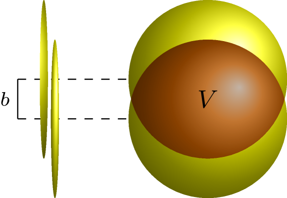
Figure 1: Schematic representation of a nucleus-nucleus collision at impact parameter $b$. The left part shows the incoming nuclei just before the collision, flattened by the relativistic Lorentz contraction in the direction of motion. The right part is the view from the collision axis. Strongly-interacting matter is created in the region where the nuclei overlap, which is indicated in darker colour, and $V$ is the collision volume. Generally, smaller $b$ is associated with larger $V$.

Transient formation of a fluid in nucleus-nucleus collisions has been inferred from the observation that particles move collectively into preferred directions, implying that their motion is driven by pressure gradients inherent in a fluid. Most notably, one observes an elliptic deformation of the azimuthal distribution of outgoing particles STAR:2000ekf ; ALICE:2010suc , which originates from the almond-shape of the overlap area between the colliding nuclei (Fig. 1). These observations are reproduced by calculations using relativistic hydrodynamics to model the expansion of the fluid Gale:2013da , which have thus been established as the standard description of nucleus-nucleus collisions.

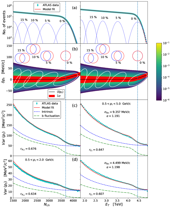
Figure 2: From top to bottom: (a) Histogram of the number of charged particles $N_{ch}$ (left), measured in the inner detector of ATLAS, and of transverse energy $E_{T}$ (right), measured in the forward and backward calorimeters, in Pb+Pb collisions at $5.02$ TeV per nucleon pair, which is the current energy of the LHC for ion beams. Solid lines are fits as superpositions of Gaussians. For the sake of illustration, contributions of collisions at fixed impact parameter $b$ corresponding to centrality fractions $0$, $5\%$, $10\%$, $15\%$ are shown as dashed lines (Methods, Sec. .1). In each plot, the vertical dashed line corresponds to the knee, defined as the average value of $N_{ch}$ or $E_{T}$ for $b=0$ collisions. (b) Joint distribution of the transverse momentum per particle $[p_{t}]$ and $N_{ch}$ (or $E_{T}$) from our model. Rather than $[p_{t}]$, we plot the deviation $\delta p_{t}\equiv[p_{t}]-\overline{p_{t0}}$, where $\overline{p_{t0}}$ is the average value of $p_{t}$ at fixed impact parameter, which is assumed to be constant. White lines are 90% confidence ellipses at fixed $b$. A schematic representation of the two colliding nuclei for these values of $b$ is also shown (Methods, Sec. .1). The black line is the mean value of $\delta p_{t}$, and the red band is the $1-\sigma$ band. (c) Variance of the transverse momentum per particle $[p_{t}]$, evaluated for particles with $0.5<p_{t}<5$ GeV$/c$, as a function of the centrality estimator. The full line corresponds to the square of the half-width of the red band in the plot just above. Symbols are ATLAS data ATLAS:2022dov . We also display separately the two contributions to the variance, Eq. (2), in our model calculation, whose sum is the full line. (d) Same as (c), but restricting the momentum range of the particles to $0.5<p_{t}<2$ GeV$/c$.

Here, we report independent evidence for the formation of a fluid, which does not involve the directions of outgoing particles, but solely their momenta. The ATLAS Collaboration at the LHC detects charged particles and measures their momentum $p$ in an inner detector which covers roughly the angular range $10^{\circ}<\theta<170^{\circ}$, where $\theta$ is the angle between the collision axis and the direction of the particle. Rather than the momentum itself, we use its projection perpendicular to the collision axis, $p_{t}\equiv p\sin\theta$, whose magnitude varies mildly with $\theta$. The observables of interest are, for every collision, the multiplicity of charged particles seen in the inner detector, denoted by $N_{ch}$, and the transverse momentum per charged particle, $(\sum p_{t})/N_{ch}$, denoted by $[p_{t}]$. $N_{ch}$ is used to estimate the centrality Back:2000gw ; Adler:2001yq ; Adler:2004zn ; ALICE:2013hur , since a more central collision, with a smaller impact parameter, produces on average more particles.

For collisions with the same $N_{ch}$, $[p_{t}]$ fluctuates from event to event. After subtracting trivial statistical fluctuations, the remaining dynamical fluctuations Adams:2003uw are very small, below 1% in central Pb+Pb collisions at the LHC Abelev:2014ckr . These dynamical fluctuations are the focus of our study. The left panel of Fig. 2 (c) displays their variance as a function of $N_{ch}$ ATLAS:2022dov . The striking phenomenon is a steep decrease, by a factor $\sim 2$, over a narrow interval of $N_{ch}$ around $3700$. This behavior is not reproduced by models of the collision in which the Pb+Pb collision is treated as a superposition of independent nucleon-nucleon collisions, such as the HIJING model Wang:1991hta , where the decrease of the variance is proportional to $1/N_{ch}$ Abelev:2014ckr ; Bhatta:2021qfk for all $N_{ch}$.

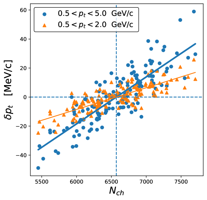
Figure 3: Scatter plot of the transverse momentum per particle $[p_{t}]$ and the charged particle multiplicity $N_{ch}$ in hydrodynamic simulations of 150 Pb+Pb collisions at 5.02 TeV and $b=0$, where $N_{ch}$ is calculated using the same acceptance cuts on $\theta$ and $p_{t}$ as in the ATLAS analysis. As in Fig. 2, we plot, rather than $[p_{t}]$ itself, the difference $\delta p_{t}\equiv[p_{t}]-\overline{p_{t}}$, where $\overline{p_{t}}$ is the value averaged over collisions. The density profile used as an initial condition to the hydrodynamic calculation fluctuates from event to event due to quantum fluctuations. Each point corresponds to a different density profile. The hydrodynamic setup is identical to that used in Ref. Bozek:2021mov (see Methods, Sec. .2). The two types of symbols correspond to different intervals for the momentum $p_{t}$ of the particles. The default analysis is done in the interval $0.5-5$ GeV$/c$, and the corresponding value of $\overline{p_{t}}$ is $1083$ MeV$/c$. The effect of narrowing the interval to $0.5-2$ GeV$/c$ is discussed at the end of this paper. As one removes particles with higher values of $p_{t}$, the average value $\overline{p_{t}}$ decreases, and is only $974$ MeV$/c$. The full lines indicate the average value $\overline{\delta p_{t}}(N_{ch},b=0)$, calculated according to Eq. (11).

We will argue that the impact parameter, $b$, plays a crucial role in this phenomenon. The relation between $N_{ch}$ and $b$ is not one-to-one, and $[p_{t}]$ depends on both quantities. In order to illustrate this dependence, we simulate 150 collisions at $b=0$ using relativistic viscous hydrodynamics, and evaluate $[p_{t}]$ and $N_{ch}$ for every collision. Figure 3 displays their distribution. The first observation is that they span a finite range: Fluctuations around the mean extend up to $\sim 15\%$ for $N_{ch}$, and to $\sim 3\%$ for $[p_{t}]$. The second observation is that there is a positive correlation between $[p_{t}]$ and $N_{ch}$.

This correlation can be understood by means of a simple thermodynamic argument. Larger $N_{ch}$ implies a larger density $N_{ch}/V$, as the volume $V$ is essentially defined by the impact parameter, which is fixed. Thus one observes that, on average, a larger density implies a larger momentum per particle $[p_{t}]$. Relativity plays an essential role in this phenomenon. In non-relativistic thermodynamics, the momentum per particle is determined by the temperature, but the particle density is not, so they are not directly related. In a relativistic system, on the other hand, mass can be converted into kinetic energy, and temperature is the only thermodynamic parameter. It determines the momentum per particle and the density, which both increase with temperature.

The relation between this thermodynamic argument and the actual hydrodynamic simulation is not straightforward. In a hydrodynamic simulation, the temperature depends on position and time, and the system is not at rest. Its motion is determined locally by the fluid velocity. Particles are emitted after the fluid has expanded and cooled down to the point where it fragments into particles, at the so-called “freeze-out temperature”. The particle momentum is a residual thermal momentum at this temperature, boosted by the fluid velocity at the point of emission. Despite the complexity of this description, one observes numerically that the fluctuations of $[p_{t}]$ at fixed impact parameter and multiplicity are very strongly correlated with those of the energy of the fluid at the time when it thermalizes, and before it starts expanding Gardim:2020sma . This validates the thermodynamic argument outlined above.

We now discuss the implications of this phenomenon on the observed $[p_{t}]$ fluctuations. First, note that the experimental analysis is done at fixed $N_{ch}$, while our hydrodynamic simulation is done at fixed $b$. Both choices are dictated by practical reasons. Experimentally, $b$ is not measured. In the simulation, on the other hand, one must define $b$ before starting the simulation, while $N_{ch}$ is only evaluated at the end.

In order to understand experimental results, we must reason at fixed $N_{ch}$, where $b$ varies. Larger $b$ implies smaller collision volume $V$ and larger density $N_{ch}/V$, hence larger $[p_{t}]$ on average. We denote by $\overline{p_{t}}(N_{ch},b)$ the expectation value of $[p_{t}]$ at fixed $N_{ch}$ and $b$. It increases with $N_{ch}$ at fixed $b$, and with $b$ at fixed $N_{ch}$. In addition, there are fluctuations of $[p_{t}]$ even if both $N_{ch}$ and $b$ are fixed, as illustrated by the simulation in Fig. 3. We denote by ${\rm Var}(p_{t}|N_{ch},b)$ their variance. A simple calculation shows that the variance at fixed $N_{ch}$, obtained after averaging over $b$, is the sum of two positive terms:

$${\rm Var}(p_{t}|N_{ch}) = \left(\left\langle\overline{p_{t}}(N_{ch},b)^{2}\right\rangle_{b}-\left\langle\overline{p_{t}}(N_{ch},b)\right\rangle_{b}^{2}\right)$$ (2)

$$+\left\langle{\rm Var}(p_{t}|N_{ch},b)\right\rangle_{b},$$

where $\langle\cdots\rangle_{b}$ denotes an average over $b$. The first term stems from the variation of $\overline{p_{t}}(N_{ch},b)$ with $b$, and the second term is the contribution of intrinsic variance. As we shall see, both terms are of comparable magnitudes, and the first term explains the peculiar pattern observed for large $N_{ch}$.

We now carry out a quantitative calculation, which can be compared with data. First, precise information can be obtained, without any microscopic modeling, about the probability distribution of $b$ at fixed $N_{ch}$, $P(b|N_{ch})$ Das:2017ned . This is achieved by solving first the inverse problem, namely, finding the probability distribution of $N_{ch}$ for fixed $b$, $P(N_{ch}|b)$, and then applying Bayes’ theorem $P(b|N_{ch})P(N_{ch})=P(N_{ch}|b)P(b)$. Collisions at the same $b$ differ by quantum fluctuations, which originate from the wavefunctions of the incoming nuclei (in particular from the positions of nucleons at the time of impact Miller:2007ri ), from the partonic content of the nucleons Gelis:2010nm , and from the collision process itself. In nucleus-nucleus collisions, these fluctuations are small enough that the fluctuations of $N_{ch}$ around its average value at fixed $b$ are Gaussian to a good approximation. They are characterized by the mean, $\overline{N_{ch}}(b)$, and the variance, ${\rm Var}(N_{ch}|b)$.

What one measures is the distribution $P(N_{ch})$, obtained after integrating over all values of $b$, shown in Fig. 2 (a), left. We only display values of $N_{ch}$ larger than some threshold such that only 20% of the events are included, corresponding to fairly central collisions on which our analysis focuses. $P(N_{ch})$ varies mildly up to $N_{ch}\sim 3500$, then decreases steeply. By fitting it as a superposition of Gaussians, one can precisely reconstruct $\overline{N_{ch}}(b)$ and ${\rm Var}(N_{ch}|b=0)$ Yousefnia:2021cup (Methods, Sec. .1). This fit is shown in Fig. 2 (a). The “knee” of the distribution, defined as the mean value of $N_{ch}$ for collisions at $b=0$, is reconstructed precisely, and indicated as a vertical line. The steep fall of $P(N_{ch})$ above the knee gives direct access to ${\rm Var}(N_{ch}|b=0)$. [Note that the variance is only reconstructed at $b=0$, and one must resort to assumptions as to its dependence on $b$. We have checked that our results are robust with respect to these assumptions, see Methods, Secs. .1 and .4.] We refer to events above the knee as ultracentral collisions Luzum:2012wu ; CMS:2013bza . They are a small fraction of the total number of events, $0.35\%$, but ATLAS has recorded enough collisions that a few events are seen with values of $N_{ch}$ larger than the knee by $20\%$, corresponding to 4 standard deviations. Note that Poisson fluctuations contribute by less than 20% to the variance Yousefnia:2021cup , so that the fluctuations of $N_{ch}$ are mostly dynamical.

We then model the fluctuations of $[p_{t}]$. In the same way as we have assumed that the probability of $N_{ch}$ at fixed $b$ is Gaussian, we assume that the joint probability of $N_{ch}$ and $[p_{t}]$, such as displayed in Fig. 3, is a two-dimensional Gaussian (Methods, Sec. .3). It is characterized by five quantities: The mean and variance of $[p_{t}]$ and $N_{ch}$, which we denote by $\overline{p_{t}}(b)$, $\overline{N_{ch}}(b)$, ${\rm Var}(p_{t}|b)$, ${\rm Var}(N_{ch}|b)$, and the covariance or, equivalently, the Pearson correlation coefficient $r_{N_{ch}}(b)$ between $[p_{t}]$ and $N_{ch}$, which we expect to be positive as illustrated in Fig. 3. $\overline{N_{ch}}(b)$ and ${\rm Var}(N_{ch}|b)$ are obtained from the fit to $P(N_{ch})$, as explained above. The mean transverse momentum is essentially independent of centrality for the 30% most central collisions ALICE:2018hza , therefore, we assume that $\overline{p_{t}}(b)$ is independent of $b$, and we denote its value by $\overline{p_{t0}}$. Since we only evaluate the fluctuations around $\overline{p_{t0}}$, results are independent of its value. The variance ${\rm Var}(p_{t}|b)$ may have a non-trivial dependence on the impact parameter, but a smooth one. For statistical fluctuations, it is proportional to $1/N_{ch}$. We allow for a more general power-law dependence ${\rm Var}(p_{t}|b)=\sigma_{\delta p_{t}}^{2}(\overline{N_{ch}}(0)/\overline{N_{ch}}(b))^{\alpha}$, where $\sigma_{\delta p_{t}}$ and $\alpha$ are constants. Finally, we ignore the impact parameter dependence of the correlation coefficient $r_{N_{ch}}$ for simplicity.

With this Gaussian ansatz, one can evaluate analytically the quantities entering the right-hand side of Eq. (2) as a function of the parameters of the Gaussian (Methods, Sec. .3). The mean value $\overline{p_{t}}(N_{ch},b)$ increases linearly with $N_{ch}$, as illustrated in Fig. 3, while the variance is independent of $N_{ch}$. Finally, the averages over $b$ in Eq. (2) are evaluated using the probability distribution $P(b|N_{ch})$ obtained using the Bayesian method outlined above. The remaining four parameters are fitted to ATLAS data: $\sigma_{\delta p_{t}}$ and $\alpha$ determine the magnitude of the variance and its dependence on centrality below the knee, while $r_{N_{ch}}$ determines the decrease of the variance around the knee. The data and the model fit are displayed in Fig. 2 (c) and (d) for two different intervals of $p_{t}$. The model explains precisely the observed decrease of the variance around the knee. We also show separately the two contributions to the variance, corresponding to the two terms in the right-hand side of Eq. (2). The first term is responsible for the observed pattern. It originates from impact parameter fluctuations at fixed $N_{ch}$, which become negligible in ultracentral collisions.

The effect can be understood simply by looking at the distribution of $[p_{t}]$ and $N_{ch}$, which is represented in Fig. 2 (b). The white curves represent 90% confidence ellipses at fixed impact parameter. The width of the $[p_{t}]$ distribution for fixed $N_{ch}$ is due in part to the intrinsic variance, corresponding to the vertical width of a single ellipse, and in part to the fluctuation of the impact parameter, implying that several ellipses contribute for a given $N_{ch}$. The latter contribution gradually disappears above the knee.

As a corollary, one predicts a small increase in the average transverse momentum, represented as a black line, in ultracentral collisions. This effect has already been predicted on the basis of a simple thermodynamic argument Gardim:2019brr and confirmed by detailed hydrodynamic calculations Nijs:2021clz , but no experimental confirmation of this effect has been publicly reported so far. The increase is quantitatively predicted by our model calculation.

A specificity of the ATLAS analysis is that it uses, in addition to $N_{ch}$, an alternative centrality estimator, which is the transverse energy $E_{T}$ (defined as energy multiplied by $\sin\theta$) deposited in two calorimeters located symmetrically on both sides of the collision point, which cover roughly the ranges $1^{\circ}<\theta<5^{\circ}$ and $175^{\circ}<\theta<179^{\circ}$. The analysis of the variance is repeated by sorting events according to $E_{T}$, rather than $N_{ch}$, and shown in the right panel of Fig. 2. In the same way, our model calculation can be repeated, replacing $N_{ch}$ with $E_{T}$ everywhere. This is a useful and non-trivial check of the validity of our approach. We fit the distribution $P(E_{T})$ as a superposition of Gaussians, as we do for $P(N_{ch})$, but the fit parameters differ (Methods, Sec. .1). Even though the distributions of $N_{ch}$ and $E_{T}$ look similar in shape (Fig. 2 (a)), the fall above the knee is steeper for $E_{T}$ than for $N_{ch}$, and there are only $0.26\%$ of events above the knee for $E_{T}$, as opposed to $0.35\%$ for $N_{ch}$. It is interesting to notice that despite this significant difference, the decrease of the variance observed by ATLAS (panels (c) and (d)) still occurs around the knee. The other parameters in our calculation are $\sigma_{\delta p_{t}}$ and $\alpha$, which determine the dependence of the variance of $[p_{t}]$ on impact parameter. These are by construction independent of whether one classifies events according to $N_{ch}$ or $E_{T}$. We determine the values that give the best agreement with $N_{ch}$ and $E_{T}$-based data (Methods Sec. .4). The last fit parameter is the Pearson correlation coefficient $r_{E_{T}}$ between $[p_{t}]$ and $E_{T}$, which need not coincide with $r_{N_{ch}}$ and is fitted independently. Note that $r_{N_{ch}}$ corresponds to the correlation between $[p_{t}]$ and $N_{ch}$ for the same particles, while $r_{E_{T}}$ represents the correlation between $[p_{t}]$ and the $E_{T}$ measured in a different angular windows. One therefore expects $r_{E_{T}}<r_{N_{ch}}$, which is confirmed by our fit. Values, however, are very similar, which shows that particle deposition in different $\theta$ windows is very strongly correlated.

Finally, another innovative aspect of the ATLAS analysis is that it studies how the fluctuations of $[p_{t}]$ change with the interval in $p_{t}$. The default analysis is done by including all particles in the range $0.5<p_{t}<5$ GeV$/c$ (particles with $p_{t}<0.5$ GeV$/c$ are not seen, and the very few particles with $p_{t}>5$ GeV$/c$ are thought to be associated with jets, and irrelevant for the study of collective behaviour), but the analysis is also done by keeping only particles in the range $0.5<p_{t}<2$ GeV$/c$. One thus excludes a small fraction of the particles, of order $7\%$. The striking observation is that the variance decreases by a factor $\sim 4$, as can be seen by comparing panels (c) and (d) of Fig. 2. Remarkably, the same phenomenon is observed in the hydrodynamic simulation. One sees in Fig. 3 that the typical magnitude of $\delta p_{t}$ is smaller by a factor $\sim 2$ for the smaller $p_{t}$ interval. Numerically, we find that the variance, which is the average value of $\delta p_{t}^{2}$, decreases by a factor $4.3\pm 0.2$, compatible with the ATLAS result. This result can be understood simply (Methods Sec. .5). A fluctuation in the fluid velocity entails a global fluctuation of the $p_{t}$ distribution, and has a larger effect on the tail of the distribution. The observed dependence of the variance on the $p_{t}$ selection is a further piece of evidence that supports the hydrodynamic origin of $[p_{t}]$ fluctuations.

We have shown that the impact parameter $b$ plays a crucial role in explaining the ATLAS data on $[p_{t}]$ fluctuations. It is worth emphasizing that $b$ is the only classical parameter characterizing a collision, in the sense that its quantum uncertainty $\delta b$ is negligible. Heisenberg’s uncertainty principle gives $\delta b=\hbar/P$, where $P$ is the total momentum of the nucleus. For a Pb+Pb collision at the LHC, $\delta b\sim 4\times 10^{-7}$ fm, which is negligible compared to the range spanned by $b$, of order 15 fm for inelastic collisions. Impact parameter determines the geometry, and is an essential ingredient in the hydrodynamic description. In the same way as elliptic flow is driven by the fluctuations of its orientation, transverse momentum fluctuations are determined by the fluctuations of its magnitude.

Methods

.1 Bayesian reconstruction of impact parameter

We denote generically by $N$ the observable used as a centrality estimator, which can be either $N_{ch}$ or $E_{T}$. We assume that the distribution of $N$ at fixed $b$ is Gaussian:

$$P(N|b)=\frac{1}{\sqrt{2\pi{\rm Var}(N|b)}}\exp\left(-\frac{\left(N-\overline{N}(b)\right)^{2}}{2{\rm Var}(N|b)}\right).$$ (3)

We introduce as an auxiliary variable the cumulative distribution of $b$ Das:2017ned :

$$c_{b}=\int_{0}^{b}P(b^{\prime})db^{\prime}\simeq\frac{\pi b^{2}}{\sigma},$$ (4)

where $P(b)\simeq 2\pi b/\sigma$ is the probability distribution of $b$, and $\sigma$ is the cross section of the nucleus-nucleus collision. $c_{b}$, which lies between $0$ and $1$, is usually called the centrality fraction. With this auxiliary variable, the probability distribution of $N$ can be written as $P(N)=\int_{0}^{1}P(N|b)dc_{b}$. We assume that $\overline{N}(b)$ is a smooth function of $c_{b}$, which we parametrize as the exponential of a polynomial. A polynomial of degree $3$ is enough to obtain excellent fits to $P(N)$ in the chosen range:

$$\overline{N}(b)=\overline{N}(0)\exp\left(-\sum_{i=1}^{3}a_{i}(c_{b})^{i}\right).$$ (5)

Similarly, the variance ${\rm Var}(N|b)$ is assumed to vary smoothly with $c_{b}$. By default, we assume that ${\rm Var}(N|b)/\overline{N}(b)$ is constant. The parameters are fitted to the distribution $P(N_{ch})$ and $P(E_{T})$ measured by ATLAS in Pb+Pb collisions. The fit is in agreement with data within 2%. We have also tested two alternative scenarios, assuming either that ${\rm Var}(N|b)$ is constant or that the ratio ${\rm Var}(N|b)/\overline{N}(b)^{2}$ is constant. The quality of the fit is as good and the fit parameters are essentially unchanged, as shown in Table 1.

$N$	$N_{ch}$	$E_{T}$
$\overline{N}(b=0)$	$3683\pm 4$	$4.435\pm 0.003$ TeV
$\sqrt{{\rm Var}(N|b=0)}$	$168.1\pm 0.1$	$0.1433\pm 0.0001$ TeV
$a_{1}$	$4.97\pm 0.02$	$4.83\pm 0.01$
$a_{2}$	$-5.58\pm 0.03$	$-4.59\pm 0.01$
$a_{3}$	$15.7\pm 0.12$	$13.1\pm 0.07$

Table 1: Values of fit parameters for Pb+Pb collisions at center-of-mass energy $5.02$ TeV per nucleon pair. For each parameter, the central value is that obtained by assuming that the variance is proportional to the mean, and the error bars reflect the changes when one assumes instead that the variance is constant, or proportional to the square of the mean.

The largest source of error in extracting information about impact parameter from data is a global normalization since it is difficult to evaluate experimentally which fraction of the cross-section is seen in detectors ALICE:2013hur . We ignore this issue here, since we are interested in ultracentral collisions. When we write that we use the 20% most central events, we mean that we use the 20% most central of the events that are actually seen in the detector. The overlapping circles in Fig. 2 (b) are a schematic representation of the colliding Pb nuclei, with radius $R=6.62$ fm, and the values of $b$ are calculated assuming that ATLAS sees approximately 90% of the inelastic events, and that the total Pb+Pb cross section is $767$ fm².

.2 Hydrodynamic simulations

The setup of our hydrodynamic calculation is identical to that of Ref. Bozek:2021mov . We use a boost-invariant version of the hydrodynamic code MUSIC Paquet:2015lta with the default freeze-out temperature $T_{f}=135$ MeV. We use a constant shear viscosity to entropy density ratio $\eta/s=0.12$, and the bulk viscosity is set to zero. The initial entropy distributions are taken from the TRENTO model Moreland:2014oya with default parameter values. The most important parameter is the parameter $p$ which defines the dependence of the density on the thickness functions of incoming nuclei, which is set to $p=0$, corresponding to a geometric mean. The normalization of the density is adjusted so as to reproduce the charged multiplicity measured by ALICE in Pb+Pb collisions at $5.02$ TeV ALICE:2015juo . Despite this normalization, we overestimate the charged multiplicity seen by ATLAS almost by 50%. The main reason is not all charged particles are seen, even within the specified angular and $p_{t}$ range, and the data are not corrected for the reconstruction efficiency. In addition, we expect deviations between the model and data for two reasons. First, hydrodynamic models typically underestimate the pion yield at low $p_{t}$ Grossi:2021gqi ; Guillen:2020nul . Since the calculation is adjusted to reproduce the total charged multiplicity, which is dominated by pions, this implies in turn that it should overestimate the yield for $p_{t}>0.5$ GeV/c, which is the range where it is measured by ATLAS. Second, our hydrodynamic calculation assumes that the momentum distribution is independent of rapidity. In reality, it is maximum near mid-rapidity, in the region covered by the ALICE acceptance. This should also lead to slightly overestimating the multiplicity seen by ATLAS, whose inner detector covers a broader range in rapidity.

Our hydrodynamic calculation also overestimates the variance of $[p_{t}]$ fluctuations. Using the results in Fig. 3, we obtain $\sqrt{{\rm Var}(p_{t})}=18.2\pm 1.2$ MeV$/c$ ($8.8\pm 0.6$ MeV$/c$) for $0.5<p_{t}<5$ GeV$/c$ ($0.5<p_{t}<2$ GeV$/c$), larger by a factor $2$ than the values in Fig. 2. This overestimation is a common problem of hydrodynamic simulations Bozek:2012fw , and can be remedied by carefully tuning the fluctuations of the initial density profile Bozek:2017elk ; Bernhard:2019bmu ; Everett:2020xug . It is the reason why we choose to fit the magnitude of $[p_{t}]$ fluctuations to data, rather than obtain it from a hydrodynamic calculation.

Finally, our calculation overestimates the Pearson correlation coefficient $r_{N_{ch}}$. From the results in Fig. 3, we obtain $r_{N_{ch}}=0.85\pm 0.02$ and $r_{N_{ch}}=0.81\pm 0.03$ for the upper $p_{t}$ cuts at $5$ and $2$ GeV$/c$, larger than the values returned by the fit, which are below $0.7$ in Fig. 2 (c) and (d). The fact that our calculation overestimates the magnitude of $[p_{t}]$ fluctuations probably leads to overestimating its correlation with the multiplicity. In addition, the fluctuations of $N_{ch}$ in the calculation are dynamical fluctuations only. The reason is that we do not sample particles according to a Monte Carlo algorithm, but simply calculate the expectation value of $N_{ch}$ at freeze-out. By contrast, the fluctuations of $N_{ch}$ in the experiment contain a contribution from statistical fluctuations, and only 80% of the variance is of dynamical origin. The statistical Poisson fluctuations should not be correlated with the transverse momentum per particle, so they tend to reduce $r_{N_{ch}}$.

.3 Distribution of $[p_{t}]$ and $N$

We assume that the probability distribution of $[p_{t}]$ and the centrality estimator $N$ at fixed $b$ is a two-dimensional Gaussian.

$$P(\delta p_{t},N) = \frac{1}{2\pi\sqrt{(1-r^{2}){\rm Var}(p_{t}){\rm Var}(N)}}$$ (8)

$$\times\exp\left(\frac{1}{1-r^{2}}\left(-\frac{(\delta p_{t})^{2}}{2{\rm Var}(p_{t})}-\frac{\left(N-\overline{N}\right)^{2}}{2{\rm Var}(N)}\right.\right.$$

$$\left.\left.+\frac{r\left(N-\overline{N}\right)\delta p_{t}}{\sqrt{{\rm Var}(N){\rm Var}(p_{t})}}\right)\right),$$

where we have omitted the dependence on $b$ to simplify the expression, and introduced the shorthand $\delta p_{t}\equiv[p_{t}]-\overline{p_{t}(b)}$.

The linear correlation between $[p_{t}]$ and $N$ is

$$\int{\delta p_{t}(N-\overline{N})P(\delta p_{t},N)dNd\delta p_{t}}=r\sqrt{{\rm Var}(N){\rm Var}(p_{t})},$$ (9)

where integrations on both variables are from $-\infty$ to $+\infty$.

A property of the two-dimensional Gaussian distribution is that its marginal distributions, obtained upon integrating over one of the variables, are also Gaussian. Integrating (8) over $\delta p_{t}$, one recovers Eq. (3). Integrating (8) over $N$, one obtains similarly:

$$P(\delta p_{t}|b)=\frac{1}{\sqrt{2\pi{\rm Var}(p_{t}|b)}}\exp\left(-\frac{(\delta p_{t})^{2}}{2{\rm Var}(p_{t}|b)}\right),$$ (10)

where we have restored the dependence on $b$.

Another property of the two-dimensional Gaussian distribution is that if one fixes one of the variables, e.g. $N$, the probability of the other variable, e.g. $\delta p_{t}$, is also Gaussian. Its centre is:

$$\overline{\delta p_{t}}(N,b)=r(b)\sqrt{\frac{{\rm Var}(p_{t}|b)}{{\rm Var}(N|b)}}\left(N-\overline{N}(b)\right).$$ (11)

It increases linearly with $N$ due to the positive correlation, as exemplified in Fig. 3. On the other hand, the variance of the distribution of $\delta p_{t}$ at fixed $N$ is independent of $N$:

$${\rm Var}(p_{t}|N,b)=\left(1-r(b)^{2}\right){\rm Var}(p_{t}|b).$$ (12)

This equation expresses that by fixing the value of $N$, one narrows the distribution of $\delta p_{t}$ due to its positive correlation with $N$.

.4 Fitting the variance of $[p_{t}]$ fluctuations

ATLAS provides us with four sets of data for the centrality dependence of the variance, depending on whether centrality is determined with $N_{ch}$ or $E_{T}$, and whether the upper $p_{t}$ cut is $5$ or $2$ GeV$/c$. We first carry out a standard $\chi^{2}$ fit for each of these sets, where the error is the quadratic sum of the statistical and systematic errors on the data points. The three fit parameters are $\sigma_{\delta p_{t}}$ (the standard deviation of $[p_{t}]$ for $b=0$), $\alpha$ (which defines the decrease of the variance as a function of impact parameter), and the Pearson correlation coefficient $r$ between $[p_{t}]$ and the centrality estimator for fixed $b$. Consistency of our model requires that $\sigma_{\delta p_{t}}$ and $\alpha$, whose definition does not involve the centrality estimator, are identical for $N_{ch}$ and $E_{T}$ based data for a given $p_{t}$ selection. Values of $\sigma_{\delta p_{t}}$ are identical within less than $1\%$, but values of $\alpha$ differ by $6\%$ and $8\%$ respectively for the $5$ and $2$ GeV$/c$ upper $p_{t}$ cuts, with $E_{T}$-based data favouring a larger $\alpha$. We then fix the values of $\sigma_{\delta p_{t}}$ and $\alpha$ to the average values of $N_{ch}$ and $E_{T}$-based results, and redo the fits by fitting solely the Pearson correlation coefficient $r$ for each of the four sets of data. Due to the small tension between the values of $\alpha$, our fit slightly overestimates the variance for the lowest values of $N_{ch}$, and slightly underestimates it for the lowest values of $E_{T}$. This effect is of little relevance to our study which focuses on ultracentral collisions, and we have not investigated its origin.

The values of $\alpha$ are close to $1.2$, which implies that the decrease of dynamical fluctuations with impact parameter is faster than that of statistical fluctuations, for which $\alpha=1$. For the larger $p_{t}$ interval, $\sigma_{\delta p_{t}}$ is close to $10$ MeV$/c$, while the average value of $p_{t}$ is close to $1$ GeV$/c$. This corresponds to a relative dynamical fluctuation of order $1\%$ in central collisions. The values of the Pearson correlation coefficient end up being similar, between $0.6$ and $0.7$, for the four sets of data.

The results shown are obtained by assuming that the variance of the charged multiplicity is proportional to the mean, that is, ${\rm Var}(N|b)/\overline{N}(b)$ is constant. As explained in Sec. .1, we have also tested two alternative scenarios, assuming either that ${\rm Var}(N|b)$ is constant or that the ratio ${\rm Var}(N|b)/\overline{N}(b)^{2}$ is constant. We have checked that the fit to the data is as good. The values of fit parameters vary only by 2% for $\sigma_{pt}$ and by 3% for the correlation coefficient $r$.

.5 Dependence of the variance on the $p_{t}$ selection

We derive a back-of-the-envelope estimate of the dependence of the variance on the $p_{t}$ selection, which is seen by comparing panels (c) and (d) of Fig. 2, and by comparing the two sets of symbols in Fig. 3. In hydrodynamics, event-by-event fluctuations of $[p_{t}]$ stem from fluctuations of the transverse fluid velocity. Now, the momentum distribution of particles is a boosted Boltzmann distribution, so that $p_{t}$ appears in an exponential. It follows that the relative change of the $p_{t}$ distribution $f(p_{t})$ due to a small change in the fluid velocity is linear in $p_{t}$ Gardim:2019iah :

$$f(p_{t})=\overline{f(p_{t})}\left(1+(p_{t}-\overline{p_{t}})x\right),$$ (13)

where $\overline{f(p_{t})}$ denotes the $p_{t}$ distribution averaged over collision events, $\overline{p_{t}}\equiv\int p_{t}\overline{f(p_{t})}dp_{t}/\int\overline{f(p_{t})}dp_{t}$ is the average $p_{t}$, and $x$ is a random quantity which fluctuates event to event around $0$. Since one studies the variation of $[p_{t}]$ in a class of events with the same multiplicity, the integral of $f(p_{t})-\overline{f(p_{t})}$ must vanish, which is the reason why the relative fluctuation is proportional to $p_{t}-\overline{p_{t}}$, instead of just $p_{t}$.

The fluctuation in the transverse momentum per particle is obtained by integrating the spectrum (13) over the $p_{t}$ range used in the analysis:

$$\delta p_{t}=x\frac{\int_{p_{\rm min}}^{p_{\rm max}}(p_{t}-\overline{p_{t}})^{2}\overline{f(p_{t})}dp_{t}}{\int_{p_{\rm min}}^{p_{\rm max}}\overline{f(p_{t})}dp_{t}},$$ (14)

where we have assumed that the fluctuations are small enough that one can replace $f(p_{t})$ with the average distribution $\overline{f(p_{t})}$ in the denominator.

The dependence of the right-hand side of Eq. (14) on the upper bound $p_{\rm max}$ can be evaluated by replacing $\overline{f(p_{t})}$ with the spectra measured by ALICE in central Pb+Pb collisions at the same energy ALICE:2018vuu . We obtain that the right-hand side of Eq. (14) decreases by a factor $2.05$ when one lowers $p_{\rm max}$ from $5$ down to $2$ GeV$/c$, corresponding to a decrease by a factor $4.23$ of the variance, in agreement with that seen by ATLAS.

Note that in this simple model, the only parameter which can vary depending on the collision in Eq. (14) is the overall factor $x$, which sets the magnitude of the fluctuation. This can be tested in hydrodynamics. First, it is easy to check by eye in Fig. 3 that symbols of different types go in pairs, with the same $N_{ch}$ (the centrality estimator is always the charged multiplicity in the interval $0.5<p_{t}<5$ GeV$/c$, even if the analysis of $[p_{t}]$ fluctuations uses a different interval). Each pair corresponds to one collision event, and the proportionality factor $x$ in Eq. (14) fluctuates from event to event. One sees that the modification of $\delta p_{t}$ from one symbol to the other in the same pair is approximately the same factor for all events, as implied by Eq. (14).

More quantitatively, we have evaluated the Pearson correlation $r$ between the two values of $\delta p_{t}$ for each event, corresponding to the different cuts. We obtain $r=0.976\pm 0.004$. This is very close to the maximum value $r=1$ which would be implied by Eq. (14).

References

- (1) W. Busza, K. Rajagopal and W. van der Schee, Ann. Rev. Nucl. Part. Sci. 68, 339-376 (2018) doi:10.1146/annurev-nucl-101917-020852 [arXiv:1802.04801 [hep-ph]].
- (2) B. Schenke, Rept. Prog. Phys. 84, no.8, 082301 (2021) doi:10.1088/1361-6633/ac14c9 [arXiv:2102.11189 [nucl-th]].
- (3) J. Adam et al. [ALICE], Phys. Lett. B 772, 567-577 (2017) doi:10.1016/j.physletb.2017.07.017 [arXiv:1612.08966 [nucl-ex]].
- (4) F. G. Gardim, G. Giacalone, M. Luzum and J. Y. Ollitrault, Nature Phys. 16, no.6, 615-619 (2020) doi:10.1038/s41567-020-0846-4 [arXiv:1908.09728 [nucl-th]].
- (5) E. Shuryak, Prog. Part. Nucl. Phys. 53, 273-303 (2004) doi:10.1016/j.ppnp.2004.02.025 [arXiv:hep-ph/0312227 [hep-ph]].
- (6) K. H. Ackermann et al. [STAR], Phys. Rev. Lett. 86, 402-407 (2001) doi:10.1103/PhysRevLett.86.402 [arXiv:nucl-ex/0009011 [nucl-ex]].
- (7) K. Aamodt et al. [ALICE], Phys. Rev. Lett. 105, 252302 (2010) doi:10.1103/PhysRevLett.105.252302 [arXiv:1011.3914 [nucl-ex]].
- (8) C. Gale, S. Jeon and B. Schenke, Int. J. Mod. Phys. A 28, 1340011 (2013) doi:10.1142/S0217751X13400113 [arXiv:1301.5893 [nucl-th]].
- (9) ATLAS Collaboration, Accepted by Phys. Rev.C. [arXiv:2205.00039 [nucl-ex]].
- (10) B. B. Back et al. [PHOBOS], Phys. Rev. Lett. 85, 3100-3104 (2000) doi:10.1103/PhysRevLett.85.3100 [arXiv:hep-ex/0007036 [hep-ex]].
- (11) C. Adler et al. [STAR], Phys. Rev. Lett. 87, 112303 (2001) doi:10.1103/PhysRevLett.87.112303 [arXiv:nucl-ex/0106004 [nucl-ex]].
- (12) S. S. Adler et al. [PHENIX], Phys. Rev. C 71, 034908 (2005) [erratum: Phys. Rev. C 71, 049901 (2005)] doi:10.1103/PhysRevC.71.034908 [arXiv:nucl-ex/0409015 [nucl-ex]].
- (13) B. Abelev et al. [ALICE], Phys. Rev. C 88, no.4, 044909 (2013) doi:10.1103/PhysRevC.88.044909 [arXiv:1301.4361 [nucl-ex]].
- (14) J. Adams et al. [STAR], Phys. Rev. C 71, 064906 (2005) doi:10.1103/PhysRevC.71.064906 [arXiv:nucl-ex/0308033 [nucl-ex]].
- (15) B. B. Abelev et al. [ALICE], Eur. Phys. J. C 74, no.10, 3077 (2014) doi:10.1140/epjc/s10052-014-3077-y [arXiv:1407.5530 [nucl-ex]].
- (16) X. N. Wang and M. Gyulassy, Phys. Rev. D 44, 3501-3516 (1991) doi:10.1103/PhysRevD.44.3501
- (17) S. Bhatta, C. Zhang and J. Jia, Phys. Rev. C 105, no.2, 024904 (2022) doi:10.1103/PhysRevC.105.024904 [arXiv:2112.03397 [nucl-th]].
- (18) P. Bozek and R. Samanta, Phys. Rev. C 105, no.3, 034904 (2022) doi:10.1103/PhysRevC.105.034904 [arXiv:2109.07781 [nucl-th]].
- (19) F. G. Gardim, G. Giacalone, M. Luzum and J. Y. Ollitrault, Nucl. Phys. A 1005, 121999 (2021) doi:10.1016/j.nuclphysa.2020.121999 [arXiv:2002.07008 [nucl-th]].
- (20) S. J. Das, G. Giacalone, P. A. Monard and J. Y. Ollitrault, Phys. Rev. C 97, no.1, 014905 (2018) doi:10.1103/PhysRevC.97.014905 [arXiv:1708.00081 [nucl-th]].
- (21) M. L. Miller, K. Reygers, S. J. Sanders and P. Steinberg, Ann. Rev. Nucl. Part. Sci. 57, 205-243 (2007) doi:10.1146/annurev.nucl.57.090506.123020 [arXiv:nucl-ex/0701025 [nucl-ex]].
- (22) F. Gelis, E. Iancu, J. Jalilian-Marian and R. Venugopalan, Ann. Rev. Nucl. Part. Sci. 60, 463-489 (2010) doi:10.1146/annurev.nucl.010909.083629 [arXiv:1002.0333 [hep-ph]].
- (23) K. V. Yousefnia, A. Kotibhaskar, R. Bhalerao and J. Y. Ollitrault, Phys. Rev. C 105, no.1, 1 (2022) doi:10.1103/PhysRevC.105.014907 [arXiv:2108.03471 [nucl-th]].
- (24) M. Luzum and J. Y. Ollitrault, Nucl. Phys. A 904-905, 377c-380c (2013) doi:10.1016/j.nuclphysa.2013.02.028 [arXiv:1210.6010 [nucl-th]].
- (25) S. Chatrchyan et al. [CMS], JHEP 02, 088 (2014) doi:10.1007/JHEP02(2014)088 [arXiv:1312.1845 [nucl-ex]].
- (26) S. Acharya et al. [ALICE], Phys. Lett. B 788, 166-179 (2019) doi:10.1016/j.physletb.2018.10.052 [arXiv:1805.04399 [nucl-ex]].
- (27) F. G. Gardim, G. Giacalone and J. Y. Ollitrault, Phys. Lett. B 809, 135749 (2020) doi:10.1016/j.physletb.2020.135749 [arXiv:1909.11609 [nucl-th]].
- (28) G. Nijs and W. van der Schee, Phys. Rev. C 106, no.4, 044903 (2022) doi:10.1103/PhysRevC.106.044903 [arXiv:2110.13153 [nucl-th]].
- (29) J. F. Paquet, C. Shen, G. S. Denicol, M. Luzum, B. Schenke, S. Jeon and C. Gale, Phys. Rev. C 93, no.4, 044906 (2016) doi:10.1103/PhysRevC.93.044906 [arXiv:1509.06738 [hep-ph]].
- (30) J. S. Moreland, J. E. Bernhard and S. A. Bass, Phys. Rev. C 92, no.1, 011901 (2015) doi:10.1103/PhysRevC.92.011901 [arXiv:1412.4708 [nucl-th]].
- (31) J. Adam et al. [ALICE], Phys. Rev. Lett. 116, no.22, 222302 (2016) doi:10.1103/PhysRevLett.116.222302 [arXiv:1512.06104 [nucl-ex]].
- (32) E. Grossi, A. Soloviev, D. Teaney and F. Yan, Phys. Rev. D 104, no.3, 034025 (2021) doi:10.1103/PhysRevD.104.034025 [arXiv:2101.10847 [nucl-th]].
- (33) A. Guillen and J. Y. Ollitrault, Phys. Rev. C 103, no.6, 064911 (2021) doi:10.1103/PhysRevC.103.064911 [arXiv:2012.07898 [nucl-th]].
- (34) P. Bozek and W. Broniowski, Phys. Rev. C 85, 044910 (2012) doi:10.1103/PhysRevC.85.044910 [arXiv:1203.1810 [nucl-th]].
- (35) P. Bożek and W. Broniowski, Phys. Rev. C 96, no.1, 014904 (2017) doi:10.1103/PhysRevC.96.014904 [arXiv:1701.09105 [nucl-th]].
- (36) J. E. Bernhard, J. S. Moreland and S. A. Bass, Nature Phys. 15, no.11, 1113-1117 (2019) doi:10.1038/s41567-019-0611-8
- (37) D. Everett et al. [JETSCAPE], Phys. Rev. C 103, no.5, 054904 (2021) doi:10.1103/PhysRevC.103.054904 [arXiv:2011.01430 [hep-ph]].
- (38) F. G. Gardim, F. Grassi, P. Ishida, M. Luzum and J. Y. Ollitrault, Phys. Rev. C 100, no.5, 054905 (2019) doi:10.1103/PhysRevC.100.054905 [arXiv:1906.03045 [nucl-th]].
- (39) S. Acharya et al. [ALICE], JHEP 11, 013 (2018) doi:10.1007/JHEP11(2018)013 [arXiv:1802.09145 [nucl-ex]].