Resilient Output Consensus Control of Heterogeneous Multi-agent Systems against Byzantine Attacks: A Twin Layer Approach

Abstract

This paper studies the problem of cooperative control of heterogeneous multi-agent systems (MASs) against Byzantine attacks. The agent affected by Byzantine attacks sends different wrong values to all neighbors while applying wrong input signals for itself, which is aggressive and difficult to be defended. Inspired by the concept of Digital Twin, a new hierarchical protocol equipped with a virtual twin layer (TL) is proposed, which decouples the above problems into the defense scheme against Byzantine edge attacks on the TL and the defense scheme against Byzantine node attacks on the cyber-physical layer (CPL). On the TL, we propose a resilient topology reconfiguration strategy by adding a minimum number of key edges to improve network resilience. It is strictly proved that the control strategy is sufficient to achieve asymptotic consensus in finite time with the topology on the TL satisfying strongly $(2f+1)$-robustness. On the CPL, decentralized chattering-free controllers are proposed to guarantee the resilient output consensus for the heterogeneous MASs against Byzantine node attacks. Moreover, the obtained controller shows exponential convergence. The effectiveness and practicality of the theoretical results are verified by numerical examples.

I Introduction

The coordination issues of multi-agent systems (MASs) have attracted considerable attention in the robotics communities and the control societies due to its wide applications in the formation of unmanned aerial vehicles (UAVs) [1], electrical power grids [2], attitude alignment of satellites [3], aggregation behavior analysis of animals [4], etc. It is well known that leader-following consensus can be reached by sufficient local neighboring relative interactions. As the state variables of each agent cannot always be available in practice, various output feedback-based control protocols have been developed for event-triggered MASs [5], MASs with time delays [6], high-order nonlinear MASs [7], etc. It should be pointed out that these results commonly have an assumption that the networked system is homogeneous with all dynamics of coupled agents being identical. However, in real engineering applications, the networked system is usually heterogeneous. Considering this issue, the leader-following consensus of heterogeneous MASs has been studied in [8, 9, 10, 11]. In [8], distributed consensus controllers were designed to guarantee the leader-following consensus with heterogeneous input saturation. The authors in [9] investigated leader-following consensus of coupled heterogeneous harmonic oscillators that are one kind of second-order MASs based on relative position measurements. The leader-following consensus problem of heterogeneous MASs with nonlinear units and communication time-delay was studied in [10] and [11], respectively.

In practical applications, modern large-scale complex networked systems are vulnerable to breaking down when one or more nodes are compromised and become non-cooperative, which may be caused by malicious attacks on the communication network. In order to improve the safety of networks, the resilient consensus has been a vital research topic in the control system community in the presence of malicious attacks such as malicious attacks [12], Byzantine attacks [13], denial of service attacks (DoS) [14], false-data injection (FDI) attacks [15], deception attacks [16], and replay attacks [17]. The resilient control of MASs aims to develop distributed consensus protocols that provide an admissible system performance in hostile situations despite the network misbehavior. In the first study of the resilience of consensus under Byzantine attacks in [13], the problem was described abstractly in terms of a group of Byzantine generals with their troops camped in different places around an enemy city. However, some of them may be traitors who will confuse others to reach an agreement, which are referred to as Byzantine agents and Byzantine attacks. Since this pioneering work of the analysis of Byzantine attacks, several important advances towards the resilient consensus have been made in the last decades. In [18], a series of algorithms, called the Mean-Subsequence-Reduced (MSR) algorithms were developed to handle the approximate Byzantine consensus problem, in which the loyal nodes are able to achieve approximate agreement in the presence of $f$-total Byzantine faults in finite time. Then, authors in [19] put forward a continuous-time variation of the MSR algorithms, referred to as the Adversarial Robust Consensus Protocol (ARC-P), to achieve asymptotic consensus for Byzantine threat networks with constrained topology. In [20], a new topological property, named network robustness, was first introduced to measure the ability of the developed local algorithms W-MSR to succeed. These concepts have been later extended and employed to analyze second-order MASs in [21]. Furthermore, [22] investigated the consensus problem for nonlinear MASs suffering from attacks and communication delays. Besides the above works, researchers also investigate some other consensus-based settings like synchronization of linear time-invariant systems [23], distributed observers [24], distributed optimization[25], and so on.

However, besides the aforementioned works [8, 9, 10, 11], there are few results available for heterogeneous networks, which complicates the controller design since the agents with different dynamics are coupled through information exchange. In this article, we propose a hierarchical resilient framework to achieve the consensus of heterogeneous multi-agent systems against Byzantine attacks. For addressing this issue, the main contributions can be summarized as follows:

1. Inspired by the concept of digital twin, we design a double-layer resilient control architecture, including twin layer (TL) and cyber-physical layer (CPL). As the TL is deployed on the virtual space, the networked MASs are immune to Byzantine node attacks on the TL. Because of this feature of the TL, the resilient control strategy can be decomposed into the defense against Byzantine edge attacks on TL and the defense against Byzantine node attacks on CPL, as shown in Fig. 1.

2. We propose a resilient topology reconfiguration strategy by adding a minimum number of key edges to improve the network resilience of the TL. A new kind of control protocol is developed based on the above topology to achieve the distributed accurate estimation on each order of leader state.

3. A decentralized controller is designed on the CPL, which makes the tracking error exponentially attenuate to zero even against Byzantine attacks. Different from the existing work in [26], we manage to ensure both Byzantine nodes and normal nodes track the leader in the presence of Byzantine attacks. This implies that the network connectivity of the whole MASs is preserved thanks to our hierarchal approach. Thus, the cooperative control of agents could be stilled accomplished via our double-layer resilient control scheme, despite Byzantine attacks.

Notations: In this paper, $\sigma_{{\rm min}}(S)$ and $\sigma(S)$ are the minimum singular value and the spectrum of matrix $S$, respectively. $|S|$ is the cardinality of a set $S$. $\|\cdot\|$ is the Euclidean norm of a vector. Define the sets of real numbers, positive real numbers, nonnegative integers, positive integers as $\mathbb{R}$, $\mathbb{R}_{>0}$, $\mathbb{Z}_{\geq 0}$ and $\mathbb{Z}_{>0}$. The in-neighbor set and out-neighbor set denote the index sets denoted by $\mathcal{N}_{i}^{in}=\{i\in\textbf{I}\ |\ (z_{j},z_{i})\in\mathcal{E}\}$ and $\mathcal{N}_{i}^{out}=\{i\in\textbf{I}\ |\ (z_{i},z_{j})\in\mathcal{E}\}$, respectively. The Kronecker product is denoted by $\otimes$. $I_{N}\in\mathbb{R}^{N\times N}$ is the identity matrix. Denote $\textbf{I}[a,b]=\{a,a+1,\dots,b\}$ where $a<b$.

II Preliminaries

II-A Robust Graph Theory

For a group of agents, define a digraph $\mathcal{G}=(\mathcal{V},\mathcal{E},\mathcal{A})$ with $\mathcal{V}=\{0,1,\dots,N\}$, which indicates the edge set, $\mathcal{E}\subset\mathcal{V}\times\mathcal{V}$ indicates the edge set. The associated adjacency matrix is represented as $\mathcal{A}=[a_{ij}]$. An edge rooting from node $j$ and ending at node $i$ is represented by ($z_{j}$, $z_{i}$), meaning the information flow from node $j$ to node $i$. The weight of edge ($z_{j}$, $z_{i}$) is $[a_{ij}]$, and $a_{ij}>0$ when $(z_{j},z_{i})\in\mathcal{E}$, otherwise $a_{ij}=0$. $b_{i0}>0$ if there is an edge between the leader and the $i$th agent, otherwise $b_{i0}=0$. Some useful definitions of network robustness are recalled first.

Definition 1 (r-reachable set)

Consider a graph $\mathcal{G}=(\mathcal{V},\mathcal{E})$, a nonempty node subset $S\in\mathcal{V}$, We say that $\mathcal{S}$ is an $r$-reachable set if at least one node exists in set $\mathcal{S}$ with at least $r$ neighbors outside set $\mathcal{S}$.

The notion of $r$-reachable is able be expressed as follows: Let $r\in\mathbb{Z}_{>0}$, then define $\mathcal{X}_{S}\subseteq\mathcal{S}$ to be the subset of nodes in $\mathcal{S}$, that is

$$\mathcal{X}_{S}=\{i\in\mathcal{S}:|\mathcal{N}_{i}\backslash\mathcal{S}|\geq r\}.$$

Definition 2 (strongly r-robust w.r.t. $\mathcal{X}$)

Consider a graph $\mathcal{G}=(\mathcal{V},\mathcal{E})$ and a nonempty set $\mathcal{X}\subseteq\mathcal{V}$. $\mathcal{G}$ is called strongly $r$-robust w.r.t. $\mathcal{X}$ if every nonempty subset $\mathcal{Y}\subseteq\mathcal{V}\backslash\mathcal{X}$ is a $r$-reachable set.

II-B Nonsmooth Analysis

Next, we review some essential results on nonsmooth analysis, which will be used in this paper to investigate the convergence of the distributed protocols considered.

Consider the following system (possibly discontinuous)

$$\dot{x}=f(x),~{}\ x\in\mathbb{R}^{n},$$ (1)

where $f(x):\mathbb{R}^{n}\rightarrow\mathbb{R}^{n}$ is defined for every $x\in\mathbb{R}^{n}\backslash K$, where $K$ is a subset of $\mathbb{R}^{n}$ of measure zero. There exists a constant $k$ such that $\|f(x)\|\leq k$. We apprehend the corresponding solution in the sense of Filippov as the solution of an appropriate differential inclusion when the (1) has discontinuous right-hand side.

Definition 3 (Filippov Solution)

A vector $x(t)$ is a solution of (1) for $t\in[t_{a},t_{b}]$ if $x(t)$ is absolutely continuous on the time interval $[t_{a},t_{b}]$.

$$\dot{x}\in H[f](x),$$ (2)

where $H[f](x):\mathbb{R}^{n}\rightarrow 2^{\mathbb{R}_{n}}$ is defined as

$$H[f](x)\triangleq\underset{\alpha>0}{\bigcap}\ \underset{\delta\{K\}=0}{\bigcap}\hat{co}\{f(A(x,\alpha)\backslash K)\},$$ (3)

where $\bigcap_{\delta\{K\}=0}$ denotes the intersection of all sets $K$ of measure zero, $A(x,\alpha)$ denotes the ball of radius $\alpha$ centered at $x$, $\hat{co}$ denotes the convex closure.

The tangent vector of Filippov’s solution must lie in the convex closure of the vector field value in an area around the point of solution where the neighborhood becomes gradually smaller. It is important to note that the measurement zero set can be discarded under this definition. If $f(x)$ is measurable and locally bounded, then the set-valued mapping $H[f](x)$ is upper semicontinuous, compact, convex and locally bounded, so (2) has Filippov solutions for each initial condition $x_{0}$.

Definition 4 (Clarke’s Generalized Gradient [27])

Define $V(x)$ as a locally Lipschitz continuous function and define its Clarke’s generalized gradient $\partial V(x)$ as

$$\partial V(x)\triangleq co\{\lim_{i\rightarrow\infty}\nabla V(x_{i})|x_{i}\rightarrow x,x_{i}\notin\Phi_{V}\cup P\},$$ (4)

where $\nabla V$ denotes the gradient, $x_{i}$ denotes a point which converges to $x$ as $i$ tends to infinity, $\Phi_{V}$ is a set of Lebesgue measure zero which contains all points without $\nabla V$, and $P$ denotes a set of measure zero. Then we review the chain rule that allows to discriminate Lipschitz regular functions.

Theorem 1 (Chain Rule[28])

Let $x$ be a Filippov solution in (1) and $V(x(t))$ be a Lipschitz regular function. Then $V$ is absolutely continuous, and

$$\frac{{\rm d}}{{\rm d}t}V(x(t))\in\dot{\widetilde{V}}(x(t)),$$ (5)

where the set-valued Lie derivative $\dot{\tilde{V}}(x(t))$ is

$$\dot{\tilde{V}}(x(t))\triangleq\underset{\phi\in\partial V(x)}{\bigcap}\phi^{T}H[f](x).$$ (6)

Define the discontinuous “sign” function and the set-valued “SIGN” function as:

$${\rm sign}(x)=\begin{cases}1,\hfill{\rm if}\ x>0,\\ 0,\hfill{\rm if}\ x=0,\\ -1,\hfill{\rm if}\ x<0,\end{cases}$$ (7)

and

$${\rm SIGN}(x)=\begin{cases}1,\hfill{\rm if}\ x>0,\\ [-1,1],\hfill{\rm if}\ x=0,\\ -1,\hfill{\rm if}\ x<0.\end{cases}$$ (8)

III Problem Formulation

III-A System Model and Related Assumptions

For a multi-agent system consisting of $N+1$ agents, the agents assigned as followers are indexed by $\mathcal{F}=\{1,\ldots,N\}$ and the agent assigned as leader is indexed by $\mathcal{L}=\{0\}$. Then the dynamics of the followers are described as

$$\begin{cases}\dot{s}_{i}(t)=v_{i}(t),\\ \dot{v}_{i}(t)=\alpha_{s_{i}}s_{i}(t)+\alpha_{v_{i}}v_{i}(t)+u_{i}(t),\\ y_{i}(t)=s_{i}(t),\end{cases}$$ (9)

where $s_{i}\in\mathbb{R}^{m}$ , $v_{i}\in\mathbb{R}^{m}$, $u_{i}\in\mathbb{R}^{m}$ and $y_{i}\in\mathbb{R}^{m}$ are the position, velocity, control input and output of the follower, respectively. Define $x_{i}=[s_{i}^{T},v_{i}^{T}]^{T}$, $i\in\mathcal{F}$. Then we have $\dot{x}_{i}(t)=A_{i}x_{i}(t)+B_{i}u_{i}(t)$ and $y_{i}(t)=C_{i}x_{i}(t)$.

The dynamic of the leader is described as

$$\begin{cases}\dot{s}_{0}(t)=v_{0}(t),\\ \dot{v}_{0}(t)=u_{0}(t),\\ y_{0}(t)=s_{0}(t),\end{cases}$$ (10)

where $s_{0}\in\mathbb{R}^{q}$ , $v_{0}\in\mathbb{R}^{q}$, $u_{0}\in\mathbb{R}^{q}$ and $y_{0}\in\mathbb{R}^{q}$ are the position, velocity, control input and output of the leader, respectively. Define $x_{0}=[s_{0}^{T},v_{0}^{T}]^{T}$. Then we have $\dot{x}_{0}(t)=Sx_{0}(t)+Du_{0}(t)$ and $y_{0}(t)=Rx_{0}(t)$.

III-B Related Assumptions

Then we next make some assumptions.

Assumption 1

The control input $u_{0}$ is upper bounded by a positive constant $u_{\rm max}$, which means ${\rm sup}_{t\geq 0}\|u_{0}(t)\|_{\infty}\leq u_{\rm max}$.

Assumption 2

The pair ($S$, $R$) is detectable.

Assumption 3

For any $\lambda\in\sigma(S)$, it holds that

$${\rm rank}\bigg{(}\left[\begin{array}[]{ccc}A_{i}-\lambda I&B_{i}\\ C_{i}&0\\ \end{array}\right]\bigg{)}=n_{i}+q.$$

Lemma 1

([29]) Under Assumptions $1$-$3$, for each agent $i$, there exist some matrices $\Gamma_{i}$ and $\Pi_{i}$ that satisfy the following regulator equations:

$$\begin{cases}A_{i}\Pi_{i}+B_{i}\Gamma_{i}=\Pi_{i}S,\\ C_{i}\Pi_{i}-R=0.\end{cases}$$ (11)

In this paper, only a fraction of agents is pinned to the leader. For the sake of illustration, we take the agents where the leader can be directly observed as the pinned followers. The set of these pinned followers is described as set $\mathcal{V}_{p}$. On the other hand, the remaining agents are regarded as non-pinned followers and collected in set $\mathcal{V}_{np}$.

Define the following local output consensus error:

$$e_{i}(t)=y_{i}(t)-y_{0}(t).$$ (12)

Based on the above settings, the heterogeneous MASs in (9) are said to achieve cooperative Control if $\lim_{t\to\infty}e_{i}(t)=0,\forall i\in\mathcal{F}$.

III-C Byzantine Attack Model

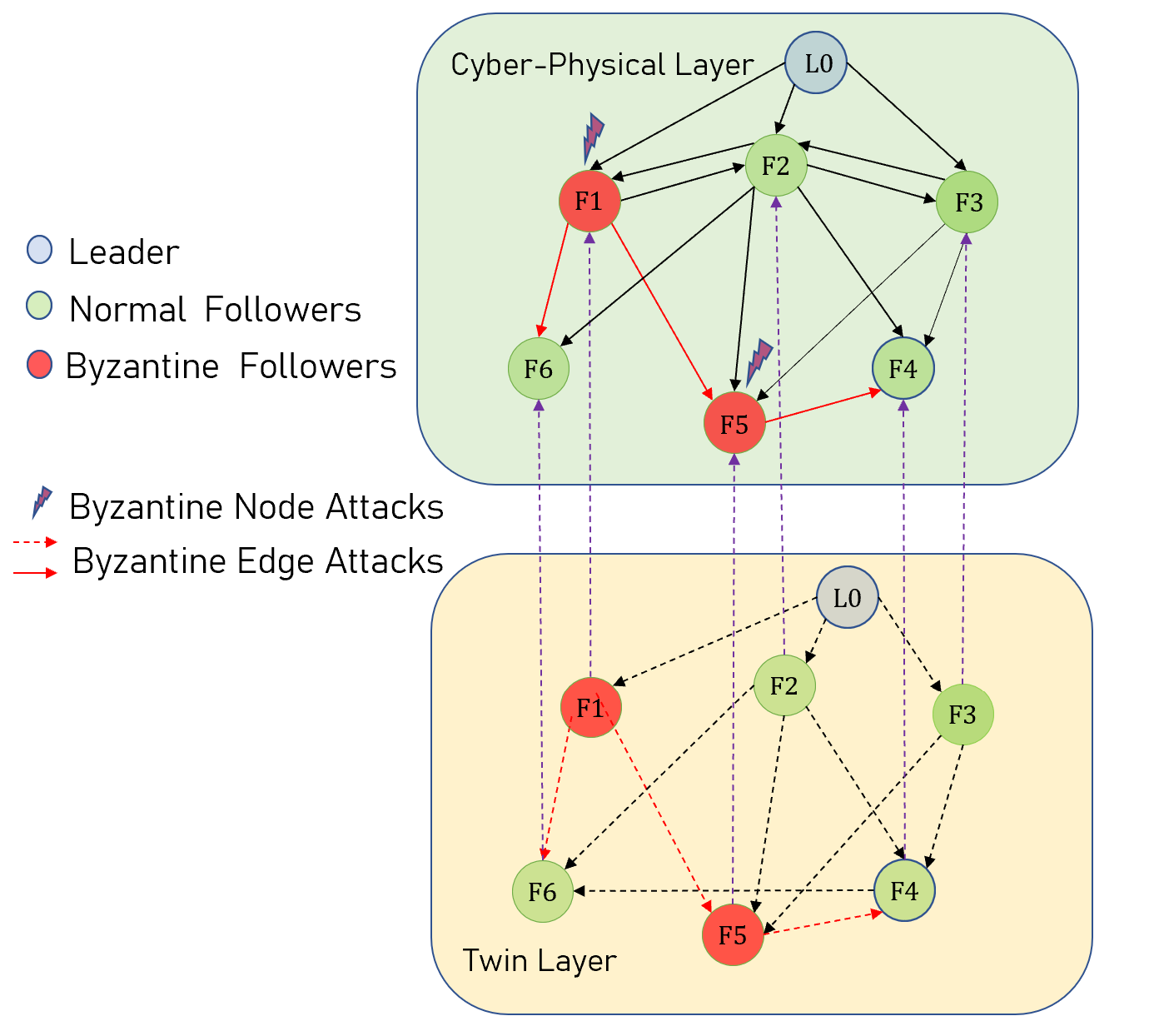
Figure 1: Distributed attack-resilient MASs against Composite Attacks: A two-layer framework.

III-C1 Edge Attacks

We consider a subset $\mathcal{B}\subseteq\mathcal{V}$ of the nodes in the network to be adversarial. We assume that the nodes are completely aware of the network topology and the system dynamics of each agent. Let us denote the agents as Byzantine agents. Then, the normal agents are collected in the set $\mathcal{K}=\{1,2,\dots,k\}$, where $k$ is the number of normal agents in the network.

Assumption 4 (f-local Attack)

There exist at most $f$ Byzantine agents in the in-neighborhood of each agent, that is, $|\mathcal{B}\cap\mathcal{N}^{in}_{i}|\leq f,\ \forall i\in\mathcal{F}$.

Here, we mainly consider the $f$-local attack model to deal with lots of Byzantine nodes in the network. It is reasonable to assume that there exist at most $f$ adjacent Byzantine nodes. Otherwise, it will be too pessimistic to protect the network.

Remark 1

The Byzantine nodes can completely understand the network topology and the system dynamics. Different from general malicious nodes in [12], the Byzantine nodes herein can send arbitrary and different false data to different in-neighbors and cooperate with other Byzantine nodes at any time. $\hfill\square$

III-C2 Node Attacks and the associated TL solution

The input signals of all Byzantine nodes on the CPL could be falsified via Byzantine node attacks. Under the influence of the Byzantine node attacks, the state of each Byzantine agent will be subverted as

$$\bar{x}_{i}(t)=x_{i}+\psi_{i}(t),\ \forall i\in\mathcal{B},$$

where $\psi_{i}(t)$ represents an unknown, time-varying, and potentially bounded signal satisfying Assumption 5.

Assumption 5

The magnitude of the Byzantine node attacks on each agent is bounded by ${\kappa_{i}}>0$, that is, $\sup_{t\in\mathbb{R}_{\geq 0}}|\psi_{i}(t)|\leq{\kappa_{i}}$, $\forall i\in\mathcal{F}$.

Note that the $i$-index set of Assumption 4 includes the Byzantine agents, apart from normal ones. This means, not only do we try to ensure that the normal agents are free from the compromised information from Byzantine edge attacks, but also we consider correcting the performance of Byzantine agents. As shown in Figure 1, a supervising layer, named TL, provides another control signals to fight against the Byzantine node attacks. With the reference signals of TL, the real input signal of each agent consists of two parts:

$$\bar{u}_{i}(t)=m_{i}(t){u}_{i}(t)+\psi_{i}(t),\ \forall i\in\mathcal{F},$$

where $m_{i}(t)$ denotes a nonzero bounded factor caused by actuator faults and $u_{i}(t)$ is the input signal (correction signal) to be designed later, which is concerned about the virtual states on the TL.

III-D Problem Formulation

Based on the above discussions, the resilient cooperative control problem of MASs, against Byzantine attacks will be summarized as follows:

Problem RC3HPB (Resilient Cooperative Control of Heterogeneous MASs against Byzantine attacks): Under Assumptions 1$\sim$5, consider the agents in (9) subject to Byzantine attacks defined in Section III-C, design distributed protocols $u_{i}$ such that the global error $e_{i}$ in (12) exponentially converges to zero. $\hfill\hfill\square$

IV Main Results

Motivated by the recently sprung-up digital twin technology, a double-layer resilient control scheme is investigated in this section, as shown in Fig. 1. Owing to the introduction of TL, the resilient control scheme against BAs can be decoupled into the defense against Byzantine edge attacks on the TL and the defense against potentially Byzantine node attacks on the CPL. More specifically, this hierarchal control scheme solves the Problem RC3HPB by employing a TL with an edge-adding strategy against Byzantine edge attacks and a decentralized adaptive controller on the CPL against potentially Byzantine node attacks.

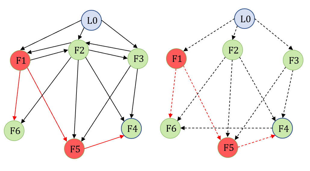
Figure 2: Topologies of the CPL and the TL.

IV-A Distributed Resilient Estimation on the TL against Byzantine edge attacks

As shown in Fig. 1, there exists a TL governor to modify the network topology by adding a minimum number of key edges to improve the network resilience of the TL topology.

IV-A1 Resilient Twins Layer Design: A Minimum Edge Number Approach

Herein, we propose a heuristic algorithm to figure out the exact topology of TL, as shown in Algorithm 1. An illustrative example for Algorithm 1 is shown in Fig. 2, whose detailed process can be found in Example 1. Notice that $\mathcal{G}$ and $\mathcal{G}_{T}$ are not necessarily the same, since the TL has certain programmable flexibility in topology. Notice that the network topology $\mathcal{G}_{T}$ except the adding edges $(v_{4},v_{6})$ on the TL is a subset of the unweighed network topology $\bar{\mathcal{G}}=(\mathcal{V},\mathcal{E})$ on the CPL. The adding edges are considered reliable since they are not affected by attackers. Denote the in-neighbor and out-neighbor sets of node $i$ on the TL as $\mathcal{N}_{T,i}^{in}$ and $\mathcal{N}_{T,i}^{out}$, respectively. Now we understand the algorithm through an example.

Algorithm 1 TL Topology Configuration Algorithm: A Minimum Edge Number Approach

Input: The topology $\mathcal{G}(\mathcal{V},\mathcal{E},\mathcal{A})$ and the parameter $f$.
Output: The TL topology $\mathcal{G}_{T}(\mathcal{V}_{T},\mathcal{E}_{T})$.

1:Initialize $\mathcal{V}$ and $\mathcal{E}$ as $\varnothing$. Initialize the sets $\mathcal{M}_{a}=\varnothing$ and $\mathcal{M}_{b}$ = $\mathcal{F}\cup\mathcal{L}$.

2:Add the leader node into $\mathcal{M}_{a}$. Update $\mathcal{M}_{b}=\mathcal{M}_{b}\backslash\mathcal{T}$.

3:while $\mathcal{M}_{a}\neq\varnothing$ do

4:     Denote the nodes pinned to $\mathcal{M}_{a}$ as $\mathcal{F}_{u}$.

5:     while $\mathcal{F}_{u}\neq\varnothing$ do

6:         for $i\in\mathcal{F}_{u}$ do

7:              if Node $i$ is pinned to the leader or at least $(2f+1)$ nodes in $\mathcal{M}_{a}$ then

8:                  Update $\mathcal{M}_{a}=\mathcal{M}_{a}\cup\{i\}$.

9:                  Update $\mathcal{F}_{u}=\mathcal{F}_{u}\backslash\{i\}$.

10:                  Update $\mathcal{V}_{T}$ as the set whose nodes are in $\mathcal{M}_{a}$.

11:                  Update $\mathcal{E}_{T}=\mathcal{E}_{T}\cup\mathcal{E}_{i}$.

12:                  Update $\mathcal{G}_{T}=(\mathcal{V}_{T},\mathcal{E}_{T})$.

13:              else

14:                  Add an edge $(z_{j},z_{i})$ from node $j\in\mathcal{M}_{a}$ to node $i$ and node $j$ pins to the minimal out-neighbors.                             

15:return The TL topology $\mathcal{G}_{T}(\mathcal{V}_{T},\mathcal{E}_{T})$.

Example 1

Consider the network topology in Fig. 1:

1. Add the leader into $\mathcal{M}_{a}$. Update $\mathcal{M}_{a}={0}$ and $\mathcal{M}_{b}=\mathcal{F}$.

2. Collect the agents pinned to $\mathcal{M}_{a}$ as $\mathcal{F}_{u}=\{1,2,3\}$. Since the nodes in $\mathcal{F}_{u}$ is pinned to the leader node, we update $\mathcal{M}_{a}=\{0,1,2,3\}$, $\mathcal{F}_{u}=\{4,5,6\}$, $\mathcal{V}_{T}=\{z_{0},z_{1},z_{2},z_{3}\}$ and $\mathcal{E}_{T}=\{(z_{0},z_{1}),(z_{0},z_{2}),(z_{0},z_{3})\}$.

3. Collect the agents pinned to $\mathcal{M}_{a}$ as $\mathcal{F}_{u}=\{4,5,6\}$.
   As only node 5 pins to at least $(2f+1)$ nodes in $\mathcal{M}_{a}$, we update $\mathcal{M}_{a}=\{0,1,2,3,5\}$, $\mathcal{F}_{u}=\{4,6\}$,
   $\mathcal{V}_{T}=\{z_{0},z_{1},z_{2},z_{3},z_{5}\}$ and $\mathcal{E}_{T}=\{(z_{0},z_{1}),(z_{0},z_{2}),\\ (z_{0},z_{3}),(z_{1},z_{5}),(z_{2},z_{5}),(z_{3},z_{5})\}$.

4. Collect the agents pinned to $\mathcal{M}_{a}$ as $\mathcal{F}_{u}=\{4,6\}$.
   Since only node 4 pins to at least $(2f+1)$ nodes in $\mathcal{M}_{a}$, we update $\mathcal{M}_{a}=\{0,1,2,3,4,5\}$, $\mathcal{F}_{u}=\{6\}$, $\mathcal{V}_{T}=\{z_{0},z_{1},z_{2},z_{3},z_{4},z_{5}\}$ and $\mathcal{E}_{T}=\{(z_{0},z_{1}),(z_{0},z_{2}),(z_{0},z_{3}),(z_{1},z_{5}),(z_{2},z_{5}),(z_{3},z_{5}),\\ (z_{2},z_{4}),(z_{3},z_{4}),(z_{5},z_{4})\}$.

5. Collect the agents pinned to $\mathcal{M}_{a}$ as $\mathcal{F}_{u}=\{6\}$. As none of node pins to the leader or at least $(2f+1)$ nodes in $\mathcal{M}_{a}$, the edge $(z_{4},z_{6})$ should be added. Then we can find that node 4 pins to at least $(2f+1)$ nodes in $\mathcal{M}_{a}$, we update $\mathcal{M}_{a}=\{0,1,2,3,4,5,6\}$, $\mathcal{F}_{u}=\{6\}$, $\mathcal{V}_{T}=\{z_{0},z_{1},z_{2},z_{3},z_{4},z_{5},z_{6}\}$ and $\mathcal{E}_{T}=\{(z_{0},z_{1}),(z_{0},z_{2}),(z_{0},z_{3}),(z_{1},z_{5}),(z_{2},z_{5}),(z_{3},z_{5}),\\ (z_{2},z_{4}),(z_{3},z_{4}),(z_{5},z_{4}),(z_{1},z_{6}),(z_{2},z_{6}),(z_{4},z_{6})\}$.

IV-A2 MSR algorithm on the TL

Then we use the MSR algorithm [18] to process the virtual state $z_{i}(t)$ on the TL. At any time $t$, each agent always makes updates as below:

1. Collect the status of all neighbor agents (except the leader if $i\in\mathcal{V}_{p}$) in a list $\Delta_{i,s}(t)$, $s=\{1,2\}$.

2. The agents in $\Delta_{i,s}(t)$ are divided into $\overline{\Delta}_{i,s}(t)$ and $\underline{\Delta}_{i,s}(t)$ as follows :

   $$\begin{split}&\overline{\Delta}_{i,s}(t)=\{j\in\Delta_{i}:z_{j,s}(t)>z_{i,s}(t)\},\\ &\underline{\Delta}_{i,s}(t)=\{j\in\Delta_{i,s}:z_{j,s}(t)<z_{i,s}(t)\},\end{split}$$

   Remove $f$ largest state values in $\overline{\Delta}_{i,s}(t)$ that are greater than $z_{i,s}(t)$. Remove all values if the number of agents in $\overline{\Delta}_{i,s}(t)$ is less than $f$.

3. Similarly, remove $f$ smallest state values in $\underline{\Delta}_{i,s}(t)$ that are lower than $z_{i,s}(t)$. Remove all values if the number of agents in $\underline{\Delta}_{i,s}(t)$ is less than $f$.

4. Denote $\Omega_{i,s}(t)$, termed as an admitting set, as the collection of agents whose values are retained after (2) and (3).

Then we formulate a distributed TL to achieve the resilient control of MASs:

$$\begin{split}\begin{cases}\dot{z}_{i,1}=&z_{i,2}-c_{1}(a_{ij}\sum_{j\in\Omega_{i,1}(t)}{\rm sign}(z_{i,1}-z_{j,1})\\ &+b_{i0}{\rm sign}(z_{i,1}-z_{0,1})),\\ \dot{z}_{i,2}=&-c_{2}(a_{ij}\sum_{j\in\Omega_{i,2}(t)}{\rm sign}(z_{i,2}-z_{j,2})\\ &+b_{i0}{\rm sign}(z_{i,2}-z_{0,2})),\end{cases}\end{split}$$ (13)

where the virtual state ${z}_{i,j}$ denotes the $j$th element of the $i$th agent’s estimation on the leader, $c$ denotes a positive gain and $z_{0}$ denotes the state of leader that means $z_{0}=x_{0}$.

We then give a sufficient condition such that the distributed asymptotical estimation on the TL can be achieved against the persistent Byzantine edge attacks:

Theorem 2

Consider a TL in (13) under Assumptions 1$\sim$4 and the $\mathcal{G}=(\mathcal{V},\mathcal{E})$ is strongly $(2f+1)$-robustness w.r.t. $\mathcal{V}_{p}$. The estimation error on the TL layer under Byzantine attacks converges into zero asymptotically, if the conditions $c_{1}>0$ and $c_{2}>u_{\rm max}$ holds.

Proof. Consider the sets $I_{s}^{M}$ and $I_{s}^{m}$ as

$$\begin{split}&I_{s}^{M}=\{i\in\mathcal{F}:z_{i,s}(t)>z_{0,s}(t)\},\\ &I_{s}^{m}=\{i\in\mathcal{F}:z_{i,s}(t)<z_{0,s}(t)\}.\end{split}$$

The nonsmooth Lyapunov function is introduced as

$$V_{s}=V_{s}^{M}+V_{s}^{m}$$ (14)

composed of terms

$$V_{s}^{M}=\sum_{i\in I_{s}^{M}}(z_{i,s}-z_{0,s}),~{}V_{s}^{m}=\sum_{i\in I_{s}^{m}}(z_{0,s}-z_{i,s}),$$

where $V_{s}^{M}$ denotes the distance between the followers with the largest state values and the leader and $V_{s}^{m}$ denotes the distance between the followers with the smallest state values and the leader and $z_{0,s}$ denotes the $s$th element of the leader.

Next, we will mainly analyze the first term of (14), since the term $V_{p}^{m}$ can be analyzed similarly.

Since $V_{p}^{M}$ is a Lipschitz regular function, we can use the chain rule given in Theorem 1 to obtain the set-valued Lie derivative as

$$\dot{\tilde{V}}_{2}^{M}(z_{2})=\underset{\phi_{2}\in\partial V_{2}^{M}(z_{2})}{\bigcap}\phi_{2}^{T}H[f](z_{2}),$$ (15)

where the generalized gradient $\partial V_{2}^{M}(z_{2})$ and collective maps $H[f](z_{2})$ are described next. The generalized gradient can be expressed in the following form

$$\partial V_{2}^{M}(z_{2})\! \subseteq\!\sum_{i\in I_{2}^{M}}\!\!\partial z_{i,2}^{M}(z_{2})\!$$ (16)

$$=\![0,\dots,Z_{k_{1}},\dots,Z_{k_{q}},\!-\!\sum_{i\in I_{2}^{M}}Z_{i},\dots,0]^{T},$$ (17)

where $Z_{i}={\rm SIGN}(z_{i,2}-z_{0,2})$ and the indices $\{k_{1},\dots,k_{q}\}$ represent the agents in the set $I_{2}^{M}$.

The composition of the $H[f](z_{2})$ is

$$H[f](z_{2})\subseteq[H[f_{0}](z_{2}),\dots,H[f_{N}](z_{2})]^{T},$$ (18)

where terms $H[f_{i}](z_{2})$ are defined as

$$H[f_{i}](z_{2}) =H\Big{[}-c_{2}\sum_{j\in\Omega_{i,2}(t)}{\rm sign}(z_{i,2}-z_{j,2})\Big{]}$$

$$\subseteq-c_{2}\sum_{j\in\Omega_{i,2}(t)}H[{\rm sign}(z_{i,2}-z_{j,2})]$$

$$=-c_{2}\sum_{j\in\Omega_{i,2}(t)}{\rm SIGN}(z_{i,2}-z_{j,2}),~{}\ i\in\mathcal{F}.$$ (19)

When the agent is a leader,

$$H[f_{0}](z_{2})=u_{0}.$$ (20)

Thus, we have

$$\phi_{2}^{T}H[f](z_{2})\subseteq\sum_{i=0}^{N}\phi_{i,2}H[f_{i}](z_{2}).$$ (21)

According to the definition of the set $I_{s}^{M}$, there exists at least a follower $i\in I_{s}^{M}$ whose status value is larger than that of the leader. In this case, we can calculate the function ${\rm SIGN}(z_{i,2}-z_{0,2})$ as

$${\rm SIGN}(z_{i,2}-z_{0,2})=\{1\},~{}i\in I_{2}^{M}.$$

Thus, we obtain the following for the $\partial V_{2}^{M}$ :

$$\partial V_{2}^{M}=[0,\dots,1,\dots,1,\dots,-|I_{2}^{M}|,\dots,0]^{T}.$$ (22)

Then, (21) is further developed as

$$\sum_{i=0}^{N}\phi_{i,2}H[f_{i}](z_{2})$$ (23)

$$= \sum_{i\in I_{2}^{M}}\Big{(}-c_{2}~{}(a_{ij}\sum_{j\in\Omega_{i,2}(t)}{\rm SIGN}(z_{i,2}-z_{j,2})$$ (24)

$$+b_{i0}{\rm SIGN}(z_{i,2}-z_{0,2}))-u_{0}\Big{)}.$$ (25)

Since the neighbors of an agent are composed of the leader and followers, it yields

$$\begin{split}&c_{2}\sum_{j\in\mathcal{N}_{i}}{\rm SIGN}(z_{i,2}-z_{j,2})\\ =&c_{2}\sum_{j\in\mathcal{N}_{i}\cap\mathcal{L}}{\rm SIGN}(z_{i,2}-z_{j,2})+c_{2}\sum_{j\in\mathcal{N}_{i}\cap\mathcal{F}}{\rm SIGN}(z_{i,2}-z_{j,2})\end{split}$$

According to (13), the set-valued Lie derivative of $V_{2}^{M}$ can be calculated as

$$\dot{\tilde{V}}_{2}^{M}(z_{2})= \sum_{i\in I_{2}^{M}}(\dot{z}_{i,2}-\dot{z}_{0,2})$$

$$= \sum_{i\in I_{2}^{M}}\Big{(}-c_{2}a_{ij}\sum_{j\in\Omega_{i,2}}{\rm SIGN}(z_{i,2}-z_{j,2})$$

$$-c_{2}b_{i0}{\rm SIGN}(z_{i,2}-z_{j,2})-u_{0}\Big{)}$$

$$\leq -c_{2}|\mathcal{V}_{p}|-c_{2}|\mathcal{V}_{np}|+u_{\rm max}|\mathcal{F}|$$

$$\leq -(c_{2}-u_{\rm max})|\mathcal{F}|.$$ (26)

We consider the worst case, that is, there exist $f$ Byzantine agents and only $f+1$ normal agents in the neighborhood. Thus, we can obtain that $-c_{2}\sum_{j\in\mathcal{N}_{i}\cap\mathcal{F}}{\rm sign}(z_{i,2}-z_{j,2})=-c_{2}$. Then, the set-valued Lie derivative can be proved as

$$-(c_{2}-u_{\rm max})|\mathcal{F}|<0.$$ (27)

Similarly, the Lie derivative of $V_{1}^{M}$ can be written as

$$\dot{\tilde{V}}_{1}^{M}= \sum_{i\in I_{1}^{M}}(\dot{z}_{i,1}-\dot{z}_{0,1})$$

$$= \sum_{i\in I_{1}^{M}}\Big{(}z_{i,2}-z_{0,2}-c_{1}\sum_{j\in\mathcal{N}_{i}\cap\mathcal{F}}{\rm SIGN}(z_{i,1}-z_{j,1})$$

$$-c_{1}\sum_{j\in\mathcal{N}_{i}\cap\mathcal{L}}{\rm SIGN}(z_{i,1}-z_{j,1})\Big{)}.$$ (28)

Notice that Eq.(IV-A2) holds, which leads to $V_{2}^{M}=0$, that is, $z_{i,2}-z_{0,2}=0$. Thus, we have

$$\dot{\tilde{V}}_{1}^{M}(z_{1}) \leq-c_{1}|\mathcal{V}_{p}|-c_{1}|\mathcal{V}_{np}|$$

$$\leq-c_{1}|\mathcal{F}|<0$$ (29)

Case 2: In this situation, the set $I_{2}^{M}$ is composed of agents that share the same values as $z_{0,2}$. Inequality still hosts when there exists at least a follower in the set $I_{2}^{M}$. The (16) can be written as

$$\partial V_{2}^{M}(z_{2}) \subseteq\sum_{i\in I_{2}^{M}}\partial V_{i,2}^{M}(z_{2})$$

$$=[0,\dots,\bar{Z},\dots,\bar{Z},-\sum_{i\in I_{2}^{M}}\bar{Z},\dots,0]^{T},$$ (30)

where $\bar{Z}={\rm SIGN}(z_{i,2}-z_{0,2})$. Recalling (21), we analyze the following dot product

$$\sum_{i=0}^{N}\phi_{i,2}H[f_{i}](z_{2})$$

$$= \sum_{i\in I_{2}^{M}}\phi_{i,2}\Big{(}-c_{2}\sum_{j\in\mathcal{N}_{i}}{\rm SIGN}(z_{i,2}-z_{j,2})\Big{)}+\phi_{0,2}u_{0}.$$ (31)

Considering the variation $[-u_{\rm max},u_{\rm max}]$ for the control input of the leader and the fact that ${\rm SIGN}(z_{i,2}-z_{j,2})\subseteq[-1,1]$, the following result holds:

$$\sum_{i=0}^{N}\phi_{i,2}H[f_{i}](z_{2})$$

$$\subseteq ~{}\phi_{0,2}u_{0}+\!\!\!\sum_{i\in I_{2}^{M}}\!\!\phi_{i,2}\Big{(}\!-c_{2}\sum_{j\in\mathcal{N}_{i}}[-1,1]+[-u_{\rm max},u_{\rm max}]\Big{)}$$

$$\subseteq ~{}\phi_{0,2}[-u_{\rm max},u_{\rm max}]$$

$$+\sum_{i\in I_{2}^{M}}\phi_{i,2}[-c_{2}|\mathcal{N}_{i}|-u_{\rm max},c_{2}|\mathcal{N}_{i}|+u_{\rm max}].$$ (32)

From the above results, we can conclude

$$\dot{\tilde{V}}_{2}^{M}(z_{2})=\{0\}.$$ (33)

A similar analysis was performed for the $V_{s}^{m}$, replacing the set $I_{s}^{M}$ with the set $I_{s}^{m}$. Then, we can obtain the same bound as

$$\begin{split}\dot{\tilde{V}}_{1}^{m}(z_{1})&\leq-c_{1}|\mathcal{F}|\\ \dot{\tilde{V}}_{2}^{m}(z_{2})&\leq-(c_{2}-u_{\rm max})|\mathcal{F}|.\end{split}$$

Recalling the fact that the time derivative $\frac{{\rm d}}{{\rm d}t}z_{2}^{M}(z_{2})\in\dot{\tilde{V}}_{2}^{M}(z_{2})$, the bound is as follows

$$\frac{\rm{d}}{\rm{d}t}V_{2}^{M}(z_{2})\leq-(c_{2}-u_{\rm max})|\mathcal{F}|.$$ (34)

Then, since the Lie derivatives of both $V_{2}^{M}$ and $V_{2}^{m}$ upper bounded by $-(c_{2}-u_{\rm max})|\mathcal{F}|$, the bound on the derivative $\frac{{\rm d}}{{\rm d}t}V_{2}(z_{2})$ can be calculated as

$$\frac{\rm{d}}{\rm{d}t}V_{2}(z_{2})\leq-2(c_{2}-u_{\rm max})|\mathcal{F}|,$$ (35)

if there exists one follower that has not tracked the leader. In the meantime, we can conclude that when all followers track the leader, the derivative ${\rm d}V_{2}/{\rm d}t$ is equal to zero. For $V_{1}$, we can obtain the analogical analysis that $\frac{{\rm d}}{{\rm d}t}V_{1}(z_{1})\leq-2c_{1}|\mathcal{F}|$.

This completes the proof. $\hfill\blacksquare$

Remark 2

Different from the existing work [30], we consider the TL that can encounter Byzantine edge attacks, rather than the completely secure layer. Compared with the traditional distributed observer [30], the TL has stronger confidentiality and higher security, which can be deployed in the cloud. Also, since TL has certain programmability in topology, the topology on the TL $\mathcal{G}_{T}$ and the topology on the CPL $\mathcal{G}$ are not necessarily the same, as shown in Fig. 2. $\hfill\square$

Theorem 3

Consider the MASs satisfying Theorem 2. Then, the cooperative consensus can be achieved in a finite-time $T_{s}$ which is upper bounded by

$$T_{s}= \frac{1}{\chi_{1}}{\rm max}\{V_{1}^{M}(z_{1}(t_{1})),V_{1}^{m}(z_{1}(t_{1}))\}$$

$$+\frac{1}{\chi_{2}}{\rm max}\{V_{2}^{M}(z_{2}(0)),V_{2}^{m}(z_{2}(0))\},$$ (36)

where $\chi_{1}=c_{1}|\mathcal{F}|$ and $\chi_{2}=(c_{2}-u_{\rm max})|\mathcal{F}|$.

Proof. Let us compute the $V_{1}^{l}(z_{1}(t_{2}))$ and $V_{2}^{l}(z_{2}(t_{1}))$ as follows:

$$V_{2}^{l}(z_{2}(t_{1})) =V_{2}^{l}(z_{2}(0))+\int_{0}^{t_{1}}\frac{{\rm d}}{{\rm d}t}(V_{2}^{l}(z_{2}(\tau))){\rm d}\tau$$

$$\leq V_{2}^{l}(z_{2}(0))-\int_{0}^{t_{1}}\chi_{2}{\rm d}\tau$$

$$\leq V_{2}^{l}(z_{2}(0))-\chi_{2}t_{1},$$ (37)

where $l\in\{m,M\}$. An upper bound in the second dimension of the convergence time is

$$T_{b}=\frac{1}{\chi_{2}}{\rm max}\{V_{2}^{M}(z_{2}(0)),V_{2}^{m}(z_{2}(0))\}.$$ (38)

Similarly, the upper bound in the first dimension is $T_{a}=\frac{1}{\chi_{1}}({\rm max}\{V_{1}^{M}(z_{1}(t_{1})),V_{1}^{m}(z_{1}(t_{1}))\})$. Since $T_{s}=T_{a}+T_{b}$, $T_{s}$ can be obtained as

$$\begin{split}T_{s}=&\frac{1}{\chi_{1}}{\rm max}\{V_{1}^{M}(z_{1}(t_{1})),V_{1}^{m}(z_{1}(t_{1}))\}\\ &+\frac{1}{\chi_{2}}{\rm max}\{V_{2}^{M}(z_{2}(0)),V_{2}^{m}(z_{2}(0))\}.\end{split}$$

This completes the proof. $\hfill\blacksquare$

IV-B Decentralized Controller on the CPL against Byzantine Node Attacks

Define the following state tracking error:

$$\varepsilon_{i}=x_{i}-\Pi_{i}z_{i},$$ (39)

and define its statelike error:

$$\bar{\varepsilon}_{i}=B_{i}^{T}P_{i}\varepsilon_{i}.$$ (40)

The $\bar{\varepsilon}_{ij}$ denotes the $j$th element of $\bar{\varepsilon}_{i}$, and $\rm{diag}(\frac{\bar{\varepsilon}_{ij}}{\sqrt{\bar{\varepsilon}_{ij}^{2}+\omega^{2}}})$ denotes a diagonal matrix with a diagonal element of $\frac{\bar{\varepsilon}_{ij}}{\sqrt{\bar{\varepsilon}_{ij}^{2}+\omega^{2}}}$. The $\hat{\kappa}_{i}$ denotes the estimate of $\kappa_{i}$, and $\tilde{\kappa}_{i}=\kappa_{i}-\hat{\kappa}_{i}$.

We then present the following control protocols:

$$u_{i} =G_{i}(\iota_{i})\varrho_{i}$$ (41)

$$\dot{\iota}_{i} =-d_{i}\bar{\varepsilon}_{i}^{T}\varrho_{i}$$ (42)

$$\varrho_{i} =K_{i}x_{i}+H_{i}z_{i}-\hat{\psi}_{i},$$ (43)

where $d_{i}$ is a positive constant and $\omega=-{\rm exp}(-\alpha_{\omega}t)$ with $\alpha_{\omega}$ being a positive constant. The $G_{i}(\iota)$ denotes a diagonal matrix with the main diagonal being Nussbaum functions. In this paper, $G_{i}(\iota_{i})$ is selected as $G_{i}(\iota_{i})=-\alpha_{i}{\rm exp}(\frac{\iota_{i}^{2}}{2})(\iota_{i}^{2}+2){\rm sin}(\iota_{i})$ with $\alpha_{i}$ being a positive const. The adaptive compensational signal is designed as follows

$$\hat{\psi}_{i} ={\rm diag}(\frac{\bar{\varepsilon}_{ij}}{|{\bar{\varepsilon}_{ij}|+\omega}})\hat{\kappa}_{i},$$ (44)

$$\dot{\hat{\kappa}}_{i} ={\rm diag}(\frac{\bar{\varepsilon}_{ij}}{{|\bar{\varepsilon}_{ij}|+\omega}})\bar{\varepsilon_{i}},$$ (45)

where ${\hat{\kappa}}_{i}$ is an adaptive updating parameter.

Theorem 4

Consider the heterogeneous MASs with (9) and (10). Problem RC3HPB can be solved via the secure TL in (13) and the decentralized controller (41)-(45), if the following condition holds simultaneously:

1. The controller gain matrices $K_{i}$ and $H_{i}$ are designed as:

   $$K_{i} =-U_{i}^{-1}B_{i}^{T}P_{i},$$ (46)

   $$H_{i} =\Gamma_{i}-K_{i}\Pi_{i},$$ (47)

   where $P_{i}$ is a positive definite matrix and satisfies the following Riccati equation:

   $$P_{i}A_{i}+A_{i}^{T}P_{i}-P_{i}B_{i}U_{i}^{-1}B_{i}^{T}P_{i}+Q_{i}=0,$$ (48)

   where $U_{i}>0$ and $Q_{i}>0$ are the symmetric matrixes.

Proof. Note that (12) can be written as

$$\begin{split}\mathrm{e}_{i}(t)&=C_{i}x_{i}(t)-Rx_{0}(t)\\ &=C_{i}x_{i}(t)-C_{i}\Pi_{i}x_{0}(t)\\ &=C_{i}(x_{i}(t)-\Pi_{i}x_{0}(t))\\ &=C_{i}\big{(}x_{i}(t)-\Pi_{i}z_{i}(t)+\Pi_{i}(z_{i}(t)-x_{0}(t))\big{)}\\ &=C_{i}\varepsilon_{i}(t)+C_{i}\Pi_{i}(z_{i}(t)-x_{0}(t)),\end{split}$$

Then we have

$$\begin{split}\|\mathrm{e}_{i}(t)\|&=\|C_{i}\varepsilon_{i}(t)+C_{i}\Pi_{i}(z_{i}(t)-x_{0}(t))\|\\ &\leq\|C_{i}\varepsilon_{i}(t)\|+\|C_{i}\Pi_{i}(z_{i}(t)-x_{0}(t))\|\\ &\leq\|C_{i}\|\|\varepsilon_{i}(t)\|+\|C_{i}\Pi_{i}\|\|(z_{i}(t)-x_{0}(t))\|.\end{split}$$

To show that $\mathrm{e}_{i}(t)$ converges to 0, in the following part, we shall prove that $\|\varepsilon_{i}(t)\|\rightarrow 0$ and $\|(z_{i}(t)-x_{0}(t))\|\rightarrow 0$ as $t\rightarrow\infty$.

According to Theorem 2, $\|z_{i}(t)-x_{0}(t)\|$ converges to 0 asymptotically.

Next, we prove that $\|\varepsilon_{i}(t)\|$ converges to 0. From (9), (10), (11), (13) and (47), we obtain the time derivative of (39) as

$$\begin{split}\dot{\varepsilon}_{i}=&\dot{x}_{i}-\Pi_{i}(Sz_{i}-c\beta_{i})\\ =&A_{i}x_{i}+B_{i}K_{i}x_{i}+B_{i}H_{i}z_{i}+B_{i}(\psi_{i}-\hat{\psi}_{i})-\Pi_{i}Sz_{i}\\ &+c\Pi_{i}\beta_{i}+B_{i}(m_{i}(t)G_{i}(\iota_{i})-1)\varrho_{i}\\ =&\bar{A}_{i}\varepsilon_{i}+B_{i}(\psi_{i}-\hat{\psi}_{i})+c\Pi_{i}\beta_{i}+B_{i}(m_{i}(t)G_{i}(\iota_{i})-1)\varrho_{i},\end{split}$$

where $\bar{A}_{i}=A_{i}+B_{i}K_{i}$ and $\beta_{i}=[\sum_{j\in\mathcal{N}_{i}}{\rm sign}(z_{i,1}-z_{j,1});\sum_{j\in\mathcal{N}_{i}}{\rm sign}(z_{i,2}-z_{j,2})]$.

Let $\bar{Q}_{i}=Q_{i}+K_{i}^{T}U_{i}K_{i}$. It can be obtained from (48) that

$$P_{i}\bar{A}_{i}+\bar{A}_{i}^{T}P_{i}=-\bar{Q}_{i}.$$ (49)

The Lyapunov function is considered as:

$$V(t)=\varepsilon_{i}^{T}P_{i}\varepsilon_{i}+\tilde{\kappa}_{i}^{T}\tilde{\kappa}_{i}.$$ (50)

The derivative of $V(t)$ can be calculated as

$$\dot{V}(t)= 2\varepsilon_{i}^{T}P_{i}\dot{\varepsilon}_{i}-2\tilde{\kappa}_{i}^{T}\dot{\hat{\kappa}}_{i}$$

$$= 2\varepsilon_{i}^{T}P_{i}(\bar{A}_{i}\varepsilon_{i}-B_{i}\hat{\psi}_{i}+B_{i}\psi_{i}+c\Pi_{i}\beta_{i})$$

$$+2\bar{\varepsilon}_{i}^{T}(m_{i}(t)G_{i}(\iota_{i})-1)\varrho_{i}-2\tilde{\kappa}_{i}^{T}\dot{\hat{\kappa}}_{i}$$

$$= \varepsilon_{i}^{T}(P_{i}\bar{A}_{i}+\bar{A}_{i}^{T}P_{i})\varepsilon_{i}+2c~{}\varepsilon_{i}^{T}P_{i}\Pi_{i}\beta_{i}$$

$$+2\varepsilon_{i}^{T}P_{i}(B_{i}\psi_{i}-B_{i}\hat{\psi}_{i})$$

$$+2\bar{\varepsilon}_{i}^{T}(m_{i}(t)G_{i}(\iota_{i})-1)\varrho_{i}-2\tilde{\kappa}_{i}^{T}\dot{\hat{\kappa}}_{i}$$

$$= -\varepsilon_{i}^{T}\bar{Q}_{i}\varepsilon_{i}+2\varepsilon_{i}^{T}P_{i}(B_{i}\psi_{i}-B_{i}\hat{\psi}_{i})$$

$$+2\bar{\varepsilon}_{i}^{T}(m_{i}(t)G_{i}(\iota_{i})-1)\varrho_{i}-2\tilde{\kappa}_{i}^{T}\dot{\hat{\kappa}}_{i}.$$ (51)

Invoking Theorem 2, we conclude that all agents can track the leader in finite time. Then, the $z_{i}-z_{j}=0$ holds in finite time, which means the sign function in (13) will equal to zero.

By using (45) and $|\bar{\varepsilon}_{ij}|\kappa_{ij}-\bar{\varepsilon}_{ij}(\frac{\bar{\varepsilon}_{ij}}{|\bar{\varepsilon}_{ij}|+\omega})\kappa_{ij}\leq\omega\kappa_{ij}\leq\omega\kappa_{\rm max}$, we can obtain

$$2\varepsilon_{i}^{T}P_{i}B_{i}(\psi_{i}-\hat{\psi}_{i})-2\tilde{\kappa}_{i}^{T}\dot{\hat{\kappa}}_{i}$$

$$\leq 2|\bar{\varepsilon}_{i}|^{T}\kappa_{i}-2\bar{\varepsilon}_{i}^{T}{\rm diag}(\frac{\bar{\varepsilon}_{ij}}{|\bar{\varepsilon}_{ij}|+\omega})\hat{\kappa}_{i}$$

$$-2(\kappa_{i}^{T}-\hat{\kappa}_{i}^{T}){\rm diag}(\frac{\bar{\varepsilon}_{ij}}{|\bar{\varepsilon}_{ij}|+\omega})\bar{\varepsilon_{i}}$$

$$\leq 2|\bar{\varepsilon}_{i}|^{T}\kappa_{i}-2\bar{\varepsilon}_{i}^{T}{\rm diag}(\frac{\bar{\varepsilon}_{ij}}{|\bar{\varepsilon}_{ij}|+\omega})\kappa_{i}$$

$$\leq 2\omega\kappa_{\rm max}.$$ (52)

where $\kappa_{i}$ is defined in Assumption 5. Substituting $\eqref{eq61}$ and $\eqref{eq36}$ into $\eqref{eq35}$ yields,

$$\dot{V}(t)\leq-\varepsilon_{i}^{T}\bar{Q}_{i}\varepsilon_{i}-\frac{2}{d_{i}}(m_{i}(t)G_{i}(\iota_{i})-1)\dot{\iota}_{i}+2\omega\kappa_{\rm max}.$$ (53)

Then, we have

$$\begin{split}\dot{V}(t)\leq-\eta\varepsilon_{i}^{T}\varepsilon_{i}(t)-\frac{2}{d_{i}}(m_{i}(t)G_{i}(\iota_{i})-1)\dot{\iota}_{i}+2\omega\kappa_{\rm max},\end{split}$$ (54)

where $\eta=\sigma_{\mathrm{min}}(\bar{Q}_{i})$. From (54), we have

$$V(t)-V(0)\leq-\eta\int_{0}^{t}\|\varepsilon_{i}(\tau)\|^{2}{\rm d}\tau-\frac{2}{d_{i}}E_{1}+E_{2},$$ (55)

where $E_{1}=\int_{0}^{t}(m_{i}(\tau)G_{i}(\iota_{i})-1)\dot{\iota}_{i}{\rm d}\tau$ and $E_{2}=\int_{0}^{t}2\omega\kappa_{\rm max}\\ {\rm d}\tau$. The $E_{2}$ in $\eqref{eq45}$ is bounded. In addition, the boundedness of $E_{1}$ can be achieved by seeking a suitable function as shown in [31]-[32].

Thus, we have

$$\|\varepsilon_{i}(t)\|^{2}\leq-\int_{0}^{t}\frac{\eta}{\sigma_{\mathrm{min}}({P}_{i})}\|\varepsilon_{i}(\tau)\|^{2}{\rm d}\tau+E,$$ (56)

where $E=\frac{1}{\sigma_{\mathrm{min}}({P}_{i})}(V(0)+{\rm sup}_{t\geq 0}(-\frac{2}{d_{i}}|E_{1}|+|E_{2}|))$. Using Bellman–Gronwall Lemma, we obtain

$$\|\varepsilon_{i}(t)\|\leq\sqrt{E}\mathrm{e}^{-\frac{\eta}{2\sigma_{\mathrm{min}}({P}_{i})}t}.$$ (57)

That is, $\|\varepsilon_{i}(t)\|$ exponentially converges to zero. Hence, the cooperative control problem for MASs (9) has been solved, which completes the proof. $\hfill\blacksquare$

Remark 3

The main merits of this work are threefold:

1. Compared with the recent work [33], this paper studies the more complex heterogeneous dynamics.

2. Different from the existing work [26] only ensuring the performance of normal agents, we manage to ensure both Byzantine agents and normal agents achieve the consensus in the presence of Byzantine attacks via our twin layer approach. Thus, we first achieve resilient control against Byzantine attacks, rather than under Byzantine attacks. $\hfill\hfill\square$

V Numerical Simulation

In this section, we employ a simulation example to verify the effectiveness of the above theoretical results.

Our goal is to achieve resilient cooperative control of heterogeneous MASs. Consider heterogeneous MASs of six agents. Their communication topology is shown in Figure. 1. The heterogeneous dynamics of (9) can be described as $\alpha_{s_{i}}=-1,\alpha_{v_{i}}=-2,i\in\textbf{I}[1,3]$ and $\alpha_{s_{i}}=-2,\alpha_{v_{i}}=-3,i\in\textbf{I}[4,6]$.

We consider the following kinds of Byzantine attacks, that is, agents 1 and 5 are Byzantine agents which satisfy $f$-local assumption, that is, Assumption 4. The Byzantine edge attacks on the TL are to replace the information among agents as:

$$e_{1,5}=\left[\begin{array}[]{ccc}t\\ 2t\\ \end{array}\right],e_{1,6}=\left[\begin{array}[]{ccc}1.5t\\ -2.5t\\ \end{array}\right],e_{5,4}=\left[\begin{array}[]{ccc}-1.5t\\ 2.5t\\ \end{array}\right].$$

where $e_{i,j}$ denotes the information flow from agent $i$ to agent $j$ falsified by the Byzantine edge attacks. Notice that $e_{1,5}(t)$, $e_{1,6}(t)$ and $e_{5,4}(t)$ are different from each other, which illustrates the difference between Byzantine attacks and other malicious attacks. The Byzantine node attacks are

$$\psi_{3}=2{\rm sin}(0.5t),~{}\psi_{5}=-2{\rm sin}(0.5t),$$

and

$$m_{i}(t)=-0.6+0.1{\rm cos}(t)$$

We conduct the resilient design of the TL. The detailed construction process of TL is summarized as Example 1 in Section IV-A. The distributed estimation performance of the TL against Byzantine edge attack is shown in Fig. LABEL:image4 and Fig. LABEL:image5. It is shown that the asymptotic performance of distributed estimation error on the TL can be achieved despite the Byzantine edge attacks.

Then, we focus on the performance of CPL with the consideration of the potential Byzantine node attacks. In light of (57), the Byzantine node attack signals satisfy Assumption 6. It can be computed from (11) that

$$\Pi_{1,2,3}=\left[\begin{array}[]{ccc}1&0\\ 0&1\\ \end{array}\right],~{}\Gamma_{1,2,3}=\left[\begin{array}[]{ccc}1&2\\ \end{array}\right],$$

$$\Pi_{4,5,6}=\left[\begin{array}[]{ccc}1&0\\ 0&1\\ \end{array}\right],~{}\Gamma_{4,5,6}=\left[\begin{array}[]{ccc}2&3\\ \end{array}\right].$$

By selecting $U_{1\sim 6}=I_{2}$ and $w=1$, it can be obtained that

$$P_{1,2,3}=\left[\begin{array}[]{ccc}4&1\\ 1&1\\ \end{array}\right],~{}P_{4,5,6}=\left[\begin{array}[]{ccc}4.90&0.90\\ 0.90&0.90\\ \end{array}\right],$$

$$K_{1,2,3}=\left[\begin{array}[]{ccc}-1&-1\\ \end{array}\right],~{}H_{1,2,3}=\left[\begin{array}[]{ccc}2&3\\ \end{array}\right],$$

$$K_{4,5,6}=\left[\begin{array}[]{ccc}-0.45&-0.45\\ \end{array}\right],~{}H_{4,5,6}=\left[\begin{array}[]{ccc}2.45&3.45\\ \end{array}\right].$$

By employing the above parameters, the cooperative control error is recorded in Fig. LABEL:image6. The exact agent error $\varepsilon_{i}$ between the CPL and the TL is depicted in Fig. LABEL:image7, which is proved to converge to zero.

VI Conclusion

In this paper, we investigate the problem of cooperative control of heterogeneous MASs in the presence of Byzantine attacks. Apart from CPL, a virtual TL is deployed on the cloud. The double-layer scheme decouples the defense strategy against Byzantine attacks into the defense against Byzantine edge attacks on the TL and the defense against Byzantine node attacks on the CPL. On the TL, we propose a resilient topology reconfiguration strategy by adding a minimum number of key edges to ensure the $(2f+1)$-robustness of network topology. A local interaction protocol based on the sign function works resiliently against Byzantine edge attacks. All the virtual state can follow the leader. On the CPL, a decentralized controller is designed against Byzantine node attacks, which ensures exponential convergence. Based on the theoretical result, the agent is achieved against Byzantine attacks. In future work, it is interesting to consider the consensus problem of MASs with nonlinear dynamics [7].

References

• [1] X. Dong, Z. Yan, R. Zhang, and Y. Zhong, “Time-varying formation tracking for second-order multi-agent systems subjected to switching topologies with application to quadrotor formation flying,” IEEE Transactions on Industrial Electronics, vol. 64, no. 6, pp. 5014–5024, 2017.
• [2] H. Cai and G. Hu, “Distributed tracking control of an interconnected leader–follower multiagent system,” IEEE Transactions on Automatic Control, vol. 62, no. 7, pp. 3494–3501, 2017.
• [3] H. Liu, Y. Tian, and F. L. Lewis, “Robust trajectory tracking in satellite time-varying formation flying,” IEEE Transactions on Cybernetics, vol. 51, no. 12, pp. 5752–5760, 2021.
• [4] R. Olfati-Saber and R. M. Murray, “Consensus problems in networks of agents with switching topology and time-delays,” IEEE Transactions on Automatic Control, vol. 49, no. 9, pp. 1520–1533, 2004.
• [5] H. Li, X. Liao, T. Huang, and W. Zhu, “Event-triggering sampling based leader-following consensus in second-order multi-agent systems,” IEEE Transactions on Automatic Control, vol. 60, no. 7, pp. 1998–2003, 2015.
• [6] A. Shariati and M. Tavakoli, “A descriptor approach to robust leader-following output consensus of uncertain multi-agent systems with delay,” IEEE Transactions on Automatic Control, vol. 62, no. 10, pp. 5310–5317, 2017.
• [7] C. C. Hua, K. Li, and X. P. Guan, “Leader-following output consensus for high-order nonlinear multiagent systems,” IEEE Transactions on Automatic Control, vol. 64, no. 3, pp. 1156–1161, 2019.
• [8] J. Fu, G. Wen, T. Huang, and Z. Duan, “Consensus of multi-agent systems with heterogeneous input saturation levels,” IEEE Transactions on Circuits & Systems II Express Briefs, vol. 66, no. 6, pp. 1053–1057, 2019.
• [9] Q. Song, F. Liu, J. Cao, A. V. Vasilakos, and Y. Tang, “Leader-following synchronization of coupled homogeneous and heterogeneous harmonic oscillators based on relative position measurements,” IEEE Transactions on Control of Network Systems, vol. 6, no. 1, pp. 13–23, 2019.
• [10] C. D. Cruz-Ancona, R. Martinez-Guerra, and C. A. Perez-Pinacho, “A leader-following consensus problem of multi-agent systems in heterogeneous networks,” Automatica, vol. 115, p. 108899, 2020.
• [11] S. Luo, X. Xu, L. Liu, and G. Feng, “Leader-following consensus of heterogeneous linear multiagent systems with communication time-delays via adaptive distributed observers,” IEEE Transactions on Cybernetics, 2021.
• [12] S. Zuo and D. Yue, “Resilient output formation containment of heterogeneous multigroup systems against unbounded attacks,” IEEE Transactions on Cybernetics, 10.1109/TCYB.2020.2998333, 2020.
• [13] L. Lamport, R. Shostak, and M. Pease, “The Byzantine Generals problem,” ACM Transactions on Programming Languages and Systems, vol. 4, no. 3, pp. 382–401, 1982.
• [14] Y. Yuan, H. Yuan, G. Lei, H. Yang, and S. Sun, “Resilient control of networked control system under DoS attacks: A unified game approach,” IEEE Transactions on Industrial Informatics, vol. 12, no. 5, pp. 1786–1794, 2016.
• [15] L. Hu, Z. Wang, Q. L. Han, and X. Liu, “State estimation under false data injection attacks: Security analysis and system protection,” Automatica, vol. 87, pp. 176–183, 2018.
• [16] Y. C. Liu, G. Bianchin, and F. Pasqualetti, “Secure trajectory planning against undetectable spoofing attacks,” Automatica, vol. 112, p. 108655, 2020.
• [17] J. Liu, T. Yin, D. Yue, H. R. Karimi, and J. Cao, “Event-based secure leader-following consensus control for multiagent systems with multiple cyber attacks,” IEEE Transactions on Cybernetics, vol. 51, no. 1, pp. 162–173, 2021.
• [18] R. M. Kieckhafer and M. H. Azadmanesh, “Reaching approximate agreement with mixed-mode faults,” IEEE Transactions on Parallel & Distributed Systems, vol. 5, no. 1, pp. 53–63, 1994.
• [19] H. J. Leblanc and X. D. Koutsoukos, “Low complexity resilient consensus in networked multi-agent systems with adversaries,” in Proceedings of 15th International Conference on Hybrid Systems: Computation and Control,, 2012, pp. 5–14.
• [20] H. J. Leblanc, H. Zhang, X. Koutsoukos, and S. Sundaram, “Resilient asymptotic consensus in robust networks,” IEEE Journal on Selected Areas in Communications, vol. 31, no. 4, pp. 766–781, 2013.
• [21] S. M. Dibaji and H. Ishii, “Consensus of second-order multi-agent systems in the presence of locally bounded faults,” Systems & Control Letters, vol. 79, pp. 23–29, 2015.
• [22] Y. Wu and X. He, “Secure consensus control for multi-agent systems with attacks and communication delays,” IEEE/CAA Journal of Automatica Sinica, vol. 4, no. 1, pp. 136–174, 2017.
• [23] H. J. Leblanc and X. Koutsoukos, “Resilient first-order consensus and weakly stable, higher order synchronization of continuous-time networked multi-agent systems,” IEEE Transactions on Control of Network Systems, vol. 5, no. 3, pp. 1219–1231, 2017.
• [24] A. Mitra and S. Sundaram, “Byzantine-resilient distributed observers for LTI systems,” Automatica, vol. 108, p. 108487, 2019.
• [25] S. Sundaram and B. Gharesifard, “Distributed optimization under adversarial nodes,” IEEE Transactions on Automatic Control, vol. 64, no. 3, pp. 1063–1076, 2017.
• [26] J. Yan, C. Deng, and C. Wen, “Resilient output regulation in heterogeneous networked systems under Byzantine agents,” Automatica, vol. 133, no. 4, p. 109872, 2021.
• [27] F. H. Clarke, Optimization and nonsmooth analysis.   SIAM, 1990.
• [28] D. Shevitz and B. Paden, “Lyapunov stability theory of nonsmooth systems,” IEEE Transactions on Automatic Control, vol. 39, no. 9, pp. 1910–1914, 1994.
• [29] J. Huang, Nonlinear Output Regulation: Theory and Applications.   SIAM, 2004.
• [30] S. Xiao and J. Dong, “Distributed fault-tolerant containment control for nonlinear multi-agent systems under directed network topology via hierarchical approach,” IEEE/CAA J Autom Sinica, vol. 8, no. 4, pp. 806–816, 2021.
• [31] C. Chen, C. Wen, Z. Liu, K. Xie, Y. Zhang, and C. P. Chen, “Adaptive consensus of nonlinear multi-agent systems with non-identical partially unknown control directions and bounded modelling errors,” IEEE Transactions on Automatic Control, vol. 62, no. 9, pp. 4654–4659, 2016.
• [32] C. Wang, C. Wen, and Y. Lin, “Adaptive actuator failure compensation for a class of nonlinear systems with unknown control direction,” IEEE Transactions on Automatic Control, vol. 62, no. 1, pp. 385–392, 2016.
• [33] A. Gusrialdi, Z. Qu, and M. A. Simaan, “Competitive interaction design of cooperative systems against attacks,” IEEE Transactions on Automatic Control, vol. 63, no. 9, pp. 3159–3166, 2018.