Computational approach to the Schottky problem

Abstract.

We present a computational approach to the classical Schottky problem based on Fay’s trisecant identity for genus $g\geq 4$. For a given Riemann matrix $\mathbb{B}\in\mathbb{H}^{g}$, the Fay identity establishes linear dependence of secants in the Kummer variety if and only if the Riemann matrix corresponds to a Jacobian variety as shown by Krichever. The theta functions in terms of which these secants are expressed depend on the Abel maps of four arbitrary points on a Riemann surface. However, there is no concept of an Abel map for general $\mathbb{B}\in\mathbb{H}^{g}$. To establish linear dependence of the secants, four components of the vectors entering the theta functions can be chosen freely. The remaining components are determined by a Newton iteration to minimize the residual of the Fay identity. Krichever’s theorem assures that if this residual vanishes within the finite numerical precision for a generic choice of input data, then the Riemann matrix is with this numerical precision the period matrix of a Riemann surface. The algorithm is compared in genus 4 for some examples to the Schottky-Igusa modular form, known to give the Jacobi locus in this case. It is shown that the same residuals are achieved by the Schottky-Igusa form and the approach based on the Fay identity in this case. In genera 5, 6 and 7, we discuss known examples of Riemann matrices and perturbations thereof for which the Fay identity is not satisfied.

1. Introduction

The classical Schottky problem is concerned with identifying Riemann matrices as period matrices of some compact Riemann surface of genus $g\geq 4$ among all symmetric matrices with positive definite imaginary part forming the Siegel halfspace $\mathbb{H}^{g}$. In this paper, we present a computational approach to this problem based on Fay’s trisecant identity [15], which is an identity between theta functions depending on the Abel maps of four arbitrary distinct points on a Riemann surface. As shown by Krichever [22], this identity only holds on Jacobians and thus gives a sharp criterion to identify the Jacobi locus in $\mathbb{H}^{g}$, namely, the subset whose elements are period matrices of some suitable Riemann surface of genus $g$. The idea is to decide for a given Riemann matrix $\mathbb{B}\in\mathbb{H}^{g}$, and having no information about the Abel map, whether it is possible to choose the arguments of the theta functions, which are $g$-dimensional vectors, such that the trisecant identity is satisfied. This is equivalent to the following optimization problem: can the vectors, corresponding to Abel maps if $\mathbb{B}$ is in the Jacobi locus, be selected in a way such that the residual of the Fay identity vanishes with numerical precision $\delta$? This would indicate that $\mathbb{B}$ is in the Jacobi locus with precision $\delta$ and that the vectors for which Fay’s identity is satisfied define Abel maps.

The Schottky problem essentially goes back to Riemann; see [28, 19, 13] for additional references and a more detailed history of the problem. The Siegel halfspace $\mathbb{H}^{g}$ of Riemann matrices has (complex) dimension $g(g+1)/2$. But the Jacobi locus of Riemann matrices, being period matrices of Riemann surfaces of genus $g$, has the (complex) dimension $3g-3$. Thus the Schottky problem to identify such matrices is non-trivial for $g\geq 4$. Schottky solved the problem in genus 4 via what is now known as the Schottky-Igusa modular form [30] (a rigorous proof was given by Igusa in [21]), a modular invariant built from theta constants, theta functions with argument equal to zero. The Schottky-Igusa form vanishes exactly on the Jacobi locus. A generalization of this form to a higher genus is not known, but see for instance [3] for attempts in this direction. Farkas, Grushevsky and Salvati Manni gave a solution to the weak Schottky problem in terms of modular invariants for arbitrary genus in [13]. This means that their modular invariant vanishes on the Jacobi locus, but as was shown for genus 5 by Donagi [11], vanishing of the invariant for some matrix $\mathbb{B}$ does not guarantee this matrix is related to a Jacobian.

Algebro-geometric approaches to integrable systems, see for instance [4, 12], not only allowed to construct quasi-periodic solutions to integrable partial differential equations (PDEs), but also proved useful in the context of the Schottly problem. Krichever’s solution of the Kadomtsev-Petviashvili (KP) equation in terms of multi-dimensional theta functions on arbitrary compact Riemann surfaces raised the question of the computability of the solutions. An effective parametrization of the solutions will not work for $g\geq 4$ exactly because of the Schottky problem. This led Novikov to conjecture that Krichever’s formula gives a solution to the KP equation if and only if the matrix $\mathbb{B}$ is in the Jacobi locus. Shiota proved this conjecture in [31]. Since it was stressed in [27] that many integrable PDEs can be solved in terms of theta functions as a consequence of Fay’s identity (2), Welters [35] conjectured that this identity holds as the Novikov conjecture just on Jacobians. This was proven by Krichever [22] and is the basis of the algorithm to be presented in this paper.

To state Fay’s identity, we consider four arbitary points on a Riemann surface $\mathcal{R}$ of genus $g$: $P_{1},P_{2},P_{3},P_{4}\in\mathcal{R}$. The Abel map

$$\alpha:\mathcal{R} \to Jac(\mathcal{R}),$$

$$P \mapsto\left(\int_{P_{0}}^{P}\omega_{1},...,\int_{P_{0}}^{P}\omega_{g}\right)\mod\Lambda,$$

is a bijective map from the surface into the Jacobian $Jac(\mathcal{R})=\mathbb{C}^{g}/\Lambda$, where $\Lambda$ is the full-rank lattice formed by the periods of the holomorphic one-forms on $\mathcal{R}$. Moreover, we consider a normalized basis $\{\omega_{1},...,\omega_{g}\}$ of differentials with respect to a symplectic basis of the first homology group $\{a_{1},b_{1},...,a_{g},b_{g}\}$, i.e., $\int_{a_{j}}\omega_{k}=\delta_{jk}$. With this choice, the matrix of $b$-periods, which has components $\mathbb{B}_{jk}=\int_{b_{j}}\omega_{k}$, is symmetric and with positive definite imaginary part. Thus, the lattice $\Lambda$ takes the form

$$\Lambda=\mathbb{Z}^{g}+\mathbb{B}\mathbb{Z}^{g}=\left\{\lambda\in\mathbb{C}^{g}\quad|\quad\lambda=\mathrm{m}+\mathbb{B}\,\mathrm{n};\quad\mathrm{m},\mathrm{n}\in\mathbb{Z}^{g}\right\}.$$

The Abel map is extended to any divisor $D=\sum_{k=1}^{N}n_{k}P_{k}$ on $\mathcal{R}$ (a divisor is a formal symbol, $n_{k}\in\mathbb{Z}$, $k=1,\ldots,N$) via $\alpha(\sum_{k=1}^{N}n_{k}P_{k})=\sum_{k=1}^{N}n_{k}\alpha(P_{k})$. Following [14] we introduce the cross ratio function ($\Theta^{*}$ is a theta function with a nonsingular odd characteristic, see (13))

(1) $$\lambda_{1234}=\frac{\Theta^{*}(\alpha(P_{1})-\alpha(P_{2}))\Theta^{*}(\alpha(P_{3})-\alpha(P_{4}))}{\Theta^{*}(\alpha(P_{1})-\alpha(P_{4}))\Theta^{*}(\alpha(P_{3})-\alpha(P_{2}))}\;,$$

which is a function on $\mathcal{R}^{4}$ that vanishes for $P_{1}=P_{2}$ and $P_{3}=P_{4}$ and has poles for $P_{1}=P_{4}$ and $P_{2}=P_{3}$. Then the following identity holds:

(2) $$\begin{split}0=&\lambda_{3124}\,\Theta(\mathrm{u}+\smallint_{P_{2}}^{P_{3}})\,\Theta(\mathrm{u}+\smallint_{P_{1}}^{P_{4}})+\lambda_{3214}\,\Theta(\mathrm{u}+\smallint_{P_{1}}^{P_{3}})\,\Theta(\mathrm{u}+\smallint_{P_{2}}^{P_{4}})\\ &-\Theta(\mathrm{u})\;\Theta(\mathrm{u}+\smallint_{P_{2}}^{P_{3}}+\smallint_{P_{1}}^{P_{4}})\;,\end{split}$$

for all $\mathrm{u}\in\mathbb{C}^{g}$, where we use the notation $\int_{P}^{Q}=\alpha(Q-P)$ as well as $\int_{P_{1}+P_{2}}^{Q_{1}+Q_{2}}=\int_{P_{1}}^{Q_{1}}+\int_{P_{2}}^{Q_{2}}=\alpha(Q_{1}+Q_{2}-P_{1}-P_{2})$.

With the binary addition theorem (16) for theta functions, we get for (2)

(3) $$\lambda_{3124}\Theta\left[\epsilon/2\atop 0\right]\left(\int_{P_{2}+P_{4}}^{P_{1}+P_{3}},2\mathbb{B}\right)+\lambda_{3214}\Theta\left[\epsilon/2\atop 0\right]\left(\int_{P_{1}+P_{4}}^{P_{2}+P_{3}},2\mathbb{B}\right)-\Theta\left[\epsilon/2\atop 0\right]\left(\int_{P_{1}+P_{2}}^{P_{3}+P_{4}},2\mathbb{B}\right)=0,$$

for all $\epsilon\in\mathbb{Z}^{g}/2\mathbb{Z}^{g}$, i.e., the $g$ dimensional vectors $\epsilon$ with components $\epsilon_{i}=0,1$, $i=1,\ldots,g$. Thus the system (3) consists of $2^{g}$ equations. We put

(4) $$X:=\frac{1}{2}\int_{P_{1}+P_{2}}^{P_{3}+P_{4}},\quad Y:=\frac{1}{2}\int_{P_{2}+P_{3}}^{P_{1}+P_{4}},\quad Z:=\frac{1}{2}\int_{P_{2}+P_{4}}^{P_{1}+P_{3}},$$

which means that the $2^{g}$ equations (3) take the form

(5) $$F_{\epsilon}(X,Y,Z):=c_{1}\Theta\big{[}\begin{smallmatrix}\epsilon/2\\ 0\end{smallmatrix}\big{]}(2Z,2\mathbb{B})+c_{2}\Theta\big{[}\begin{smallmatrix}\epsilon/2\\ 0\end{smallmatrix}\big{]}(2Y,2\mathbb{B})-\Theta\big{[}\begin{smallmatrix}\epsilon/2\\ 0\end{smallmatrix}\big{]}(2X,2\mathbb{B}),$$

where

(6) $$c_{1}=\frac{\Theta^{*}(Y-X)\Theta^{*}(Y+X)}{\Theta^{*}(Y+Z)\Theta^{*}(Y-Z)},\quad c_{2}=\frac{\Theta^{*}(X+Z)\Theta^{*}(X-Z)}{\Theta^{*}(Y+Z)\Theta^{*}(Y-Z)}.$$

In this paper we use equation (3) in the following way: we choose $X$, $Y$, $Z$ to be in the fundamental domain given by

(7) $$U_{\mathbb{B}}:=\left\{\mathrm{z}\in\mathbb{C}^{g}\quad|\quad\mathrm{z}=\mathrm{p}+\mathbb{B}\,\mathrm{q},\quad p_{i},q_{i}\in[-1/2,1/2],\quad i=1,\ldots,g\right\}.$$

In other words, an arbitrary point of the Jacobian can be given in terms of the $(p_{i},q_{i})$, which are called characteristics. Thus, the function $F$ with components (5) has the form $F:U^{3}_{\mathbb{B}}\subset\mathbb{C}^{3g}\to\mathbb{C}^{2^{g}}$, where $U^{3}_{\mathbb{B}}$ is a compact subset, and it is known from Fay’s identity, see [27], that if $\mathbb{C}^{g}/\Lambda$ is a Jacobian the set of zeros of $F$ is 4-dimensional, and it is parametrized according to (4). However, we are interested in general $\mathbb{C}^{g}/\Lambda$ where the notion of an Abel map is unknown; therefore, the zeros of $F$ cannot be determined through (4). Thus, if we fix for $X$, $Y$, $Z$ the first components and for instance the second component of $X$, the function $F$ can be seen as a function of $\mathbf{x}$, the vector built from the remaining components of $X$, $Y$, $Z$ of dimension $3g-4$. According to Krichever’s theorem, this function vanishes for generic values of $X_{1,2}$, $Y_{1}$ and $Z_{1}$ for a certain choice of the vector $\mathbf{x}$ if and only if $\mathbb{B}$ is in the Jacobi locus. In the context of the Schottky problem, the task is to find the zero of $F(X,Y,Z)$ in the space of dimension $3g-4$ by varying $\mathbf{x}$. If the residual is smaller than the numerical accuracy $\delta$, then the matrix is within numerical precision in the Jacobi locus. Since $F$ is a locally holomorphic function of $X$, $Y$, $Z$, it is possible to find the zero with a standard Newton iteration as will be shown for examples in genus $g\leq 7$.

The paper is organized as follows: In section 2, we summarize basic definitions regarding theta functions, the Siegel fundamental domain and the Schottky-Igusa form. In section 3 we present the numerical algorithms. In section 4, we consider known examples in genus 4 and compare our algorithm to the Schottky-Igusa form. We show that both the Schottky-Igusa form and the approach based on the Fay identity yield the same residuals for the studied examples. This means they identify the Jacobi locus with the same numerical accuracy. In section 5, we consider examples in genera 5, 6 and 7. We add some concluding remarks in section 6. A pseudo code for the algorithm is given in the appendix.

2. Preliminaries

In this section, we summarize some theoretical facts needed in the following to numerically address the Schottky problem.

2.1. Jacobians and principally polarized Abelian varieties

Let $\mathbb{H}^{g}$ be the space of $g\times g$ complex symmetric matrices with positive definite imaginary part called the Siegel halfspace. The Riemann theta function is given by the series

(8) $$\Theta(\mathrm{z},\mathbb{B})=\sum_{\mathrm{N}\in\mathbb{Z}^{g}}\exp(\pi\mathrm{i}\langle\mathrm{N},\mathbb{B}\mathrm{N}\rangle+2\pi\mathrm{i}\langle\mathrm{N},\mathrm{z}\rangle)$$

with $\mathrm{z}\in\mathbb{C}^{g}$ and where $\left\langle\cdot,\cdot\right\rangle$ denotes the Euclidean scalar product $\left\langle\mathrm{N},\mathrm{z}\right\rangle=\sum_{i=1}^{g}\mathrm{N}_{i}\mathrm{z}_{i}$. Since $\mathbb{B}\in\mathbb{H}^{g}$, the series (8) converges uniformly for all $\mathrm{z}\in\mathbb{C}^{g}$; thus it is an entire function.

The Siegel space parametrizes the set of principally polarized Abelian varieties (PPAV) via the assignment $\mathbb{B}\mapsto(\mathcal{A}_{\mathbb{B}},\Theta_{\mathbb{B}})$, where the complex torus has the form $\mathcal{A}_{\mathbb{B}}=\mathbb{C}^{g}/(\mathbb{Z}^{g}+\mathbb{B}\mathbb{Z}^{g})$ and $\Theta_{\mathbb{B}}$ is the divisor of the theta function (8) (the set of zeros of the theta function), which is a well-defined subvariety of $\mathcal{A}_{\mathbb{B}}$ because of its quasi-periodicity properties (15). In the following, we refer to the Riemann matrix $\mathbb{B}$ and the PPAV $(\mathcal{A}_{\mathbb{B}},\Theta_{\mathbb{B}})$ interchangeably.

In the special case where $\mathbb{B}$ is the period matrix of some Riemann surface $\mathcal{R}$ (which is only unique up to a modular transformation), its associated PPAV is known as the Jacobian $Jac(\mathcal{R})$ of $\mathcal{R}$.

2.2. Symplectic transformations

Two Riemann matrices $\mathbb{B},\tilde{\mathbb{B}}\in\mathbb{H}^{g}$ can define isomorphic PPAVs if they define equivalent complex tori and if they are principally polarized. $\mathcal{A}_{\tilde{\mathbb{B}}}$ and $\mathcal{A}_{\mathbb{B}}$ are equivalent as complex tori if there exists an invertible homomorphism $\mathbb{C}^{g}/\tilde{\Lambda}\to\mathbb{C}^{g}/\Lambda$. This is equivalent to the existence of a linear transformation $\mathcal{M}:\mathbb{C}^{g}\to\mathbb{C}^{g}$ with $\mathcal{M}(\tilde{\Lambda})=\Lambda$ and a matrix

(9) $$R=\begin{pmatrix}A&B\\ C&D\end{pmatrix}\in M_{2g}(\mathbb{Z})$$

such that

(10) $$\mathcal{M}(\tilde{\mathbb{B}},\mathbb{I}_{g})=(\mathbb{B},\mathbb{I}_{g})R^{\top},$$

holds. Additionally, in order for the principal polarization to be preserved, the condition

(11) $$\begin{pmatrix}A&B\\ C&D\end{pmatrix}^{\top}\begin{pmatrix}0_{g}&\mathbb{I}_{g}\\ -\mathbb{I}_{g}&0_{g}\end{pmatrix}\begin{pmatrix}A&B\\ C&D\end{pmatrix}=\begin{pmatrix}0_{g}&\mathbb{I}_{g}\\ -\mathbb{I}_{g}&0_{g}\end{pmatrix}$$

must be satisfied [5], which means that $R\in\text{Sp}(2g,\mathbb{Z})$. Thus, two matrices in $\mathbb{H}^{g}$ conjugated under the action of the symplectic (also called modular) group $\text{Sp}(2g,\mathbb{Z})$ define equivalent PPAVs, where the action of $\text{Sp}(2g,\mathbb{Z})$ on $\mathbb{H}^{g}$ is given by (10), which is equivalent to

(12) $$\tilde{\mathbb{B}}=R\cdot\mathbb{B}=(A\mathbb{B}+B)(C\mathbb{B}+D)^{-1},$$

which we call modular transformation. Thus, given $\mathbb{B}\in\mathbb{H}^{g}$ we can choose the most convenient symplectically equivalent $\tilde{\mathbb{B}}$ in order to perform the computations as efficiently as possible. For this we will consider Siegel’s fundamental domain.

Siegel [32] gave the following fundamental domain for the modular group:

Definition 2.1.

Siegel’s fundamental domain is the subset of $\mathbb{H}^{g}$ such that $\mathbb{B}=X+\mathrm{i}Y\in\mathbb{H}^{g}$ satisfies:

1. $|X_{nm}|\leq 1/2$, $n,m=1,\ldots,g$,

2. $Y$ is in the fundamental region of Minkowski reductions [25, 26],

3. $|\det(C\mathbb{B}+D)|\geq 1$ for all $C$, $D$ (11).

2.3. Theta functions

The multi-dimensional theta functions with characteristics are defined as the series,

(13) $$\Theta\big{[}\begin{smallmatrix}\mathrm{p}\\ \mathrm{q}\end{smallmatrix}\big{]}(\mathrm{z},\mathbb{B})=\sum\limits_{\mathrm{N}\in\mathbb{Z}^{g}}\exp\left\{\pi\mathrm{i}\left\langle\mathrm{N}+\mathrm{p},\mathbb{B}\left(\mathrm{N}+\mathrm{p}\right)\right\rangle+2\pi\mathrm{i}\left\langle\mathrm{N}+\mathrm{p},\mathrm{z}+\mathrm{q}\right\rangle\right\}\;,$$

with the characteristics $\mathrm{p}$, $\mathrm{q}\in{\mathbb{R}}^{g}$. Analogously to (8), the theta function with characteristics is an entire function on $\mathbb{C}^{g}$. If $\mathbb{B}$ is the period matrix of some Riemann surface $\mathcal{R}$, a characteristic is called singular if the corresponding theta function vanishes identically on $\mathcal{R}$.

Of special interest are half-integer characteristics with $2\mathrm{p},2\mathrm{q}\in\mathbb{Z}^{g}$. Such a characteristic is called even if $4\langle\mathrm{p},\mathrm{q}\rangle=0\mbox{ mod }2$ and odd otherwise. It can be easily shown that theta functions with odd (even) characteristics are odd (even) functions of the argument $\mathrm{z}$. The theta function with characteristic is related to the Riemann theta function $\Theta$, the theta function with zero characteristic $\Theta:=\Theta\big{[}\begin{smallmatrix}0\\ 0\end{smallmatrix}\big{]}$, via

(14) $$\Theta\big{[}\begin{smallmatrix}\mathrm{p}\\ \mathrm{q}\end{smallmatrix}\big{]}(\mathrm{z},\mathbb{B})=\Theta(\mathrm{z}+\mathbb{B}\mathrm{p}+\mathrm{q})\exp\left\{\pi\mathrm{i}\left\langle\mathrm{p},\mathbb{B}\mathrm{p}\right\rangle+2\pi\mathrm{i}\left\langle\mathrm{p},\mathrm{z}+\mathrm{q}\right\rangle\right\}\;.$$

Note that from now on we will suppress the second argument of the theta functions if it is just $\mathbb{B}$ for ease of representation. From its definition, a theta function has the periodicity properties

(15) $$\Theta\big{[}\begin{smallmatrix}\mathrm{p}\\ \mathrm{q}\end{smallmatrix}\big{]}(\mathrm{z}+\mathrm{e}_{j})=\mathrm{e}^{2\pi\mathrm{i}p_{j}}\Theta\big{[}\begin{smallmatrix}\mathrm{p}\\ \mathrm{q}\end{smallmatrix}\big{]}(\mathrm{z})\;,\quad\Theta\big{[}\begin{smallmatrix}\mathrm{p}\\ \mathrm{q}\end{smallmatrix}\big{]}(\mathrm{z}+\mathbb{B}\mathrm{e}_{j})=\mathrm{e}^{-2\pi\mathrm{i}(z_{j}+q_{j})-\mathrm{i}\pi B_{jj}}\Theta\big{[}\begin{smallmatrix}\mathrm{p}\\ \mathrm{q}\end{smallmatrix}\big{]}(\mathrm{z})\;,$$

where $\mathrm{e}_{j}$ is a vector in $\mathbb{Z}^{g}$ consisting of zeros except for a $1$ in the $j$-th position. Theta functions satisfy the binary addition theorem, see for instance [34]

(16) $$\begin{split}&\Theta\big{[}\begin{smallmatrix}\alpha\\ \gamma\end{smallmatrix}\big{]}(z_{1}+z_{2},\mathbb{B})\Theta\big{[}\begin{smallmatrix}\beta\\ \delta\end{smallmatrix}\big{]}(z_{1}-z_{2},\mathbb{B})=\\ &\sum_{\epsilon\in\mathbb{Z}^{g}/2\mathbb{Z}^{g}}\Theta\big{[}\begin{smallmatrix}(\alpha+\beta)/2+\epsilon/2\\ \gamma+\delta\end{smallmatrix}\big{]}(2z_{1},2\mathbb{B})\Theta\big{[}\begin{smallmatrix}(\alpha-\beta)/2+\epsilon/2\\ \gamma-\delta\end{smallmatrix}\big{]}(2z_{2},2\mathbb{B}).\end{split}$$

The action of the modular group on theta functions is known, see for instance [4, 15, 27]. One has

(17) $$\Theta\big{[}\begin{smallmatrix}\tilde{\mathrm{p}}\\ \tilde{\mathrm{q}}\end{smallmatrix}\big{]}(\mathcal{M}^{-1}\mathrm{z},\tilde{\mathbb{B}})=k\sqrt{\det(\mathcal{M})}\exp\left(\frac{1}{2}\sum_{i\leq j}z_{i}z_{j}\frac{\partial}{\partial\mathbb{B}_{ij}}\ln\det\mathcal{M}\right)\Theta\big{[}\begin{smallmatrix}\mathrm{p}\\ \mathrm{q}\end{smallmatrix}\big{]}(\mathrm{z}),$$

where $\tilde{\mathbb{B}}$ is given by (12) and $k$ is a constant with respect to $\mathrm{z}$, and where

(18) $$\mathcal{M}=C\mathbb{B}+D,\quad\begin{pmatrix}\tilde{\mathrm{p}}\\ \tilde{\mathrm{q}}\end{pmatrix}=\begin{pmatrix}D&-C\\ -B&A\end{pmatrix}\begin{pmatrix}\mathrm{p}\\ \mathrm{q}\end{pmatrix}+\frac{1}{2}\begin{pmatrix}\mbox{diag}(CD^{\top})\\ \mbox{diag}(AB^{\top})\end{pmatrix},$$

with diag denoting the diagonal of the corresponding matrices.

2.4. Schottky-Igusa modular form

The Schottky-Igusa modular form [30, 21] is a polynomial of degree 16 in the theta constants $\Theta\big{[}\begin{smallmatrix}\mathrm{p}\\ \mathrm{q}\end{smallmatrix}\big{]}(0)$. We follow here the presentation in [8]: choose the characteristics

$$\mathrm{p}^{(1)}=\mathrm{q}^{(1)}=\frac{1}{2}\begin{pmatrix}1\\ 0\\ 1\\ 0\end{pmatrix},\quad\mathrm{p}^{(2)}=\frac{1}{2}\begin{pmatrix}0\\ 0\\ 0\\ 1\end{pmatrix},\quad\mathrm{q}^{(2)}=\frac{1}{2}\begin{pmatrix}1\\ 0\\ 0\\ 0\end{pmatrix},$$

and

$$\mathrm{p}^{(3)}=\frac{1}{2}\begin{pmatrix}0\\ 0\\ 1\\ 1\end{pmatrix},\quad\mathrm{q}^{(3)}=\frac{1}{2}\begin{pmatrix}1\\ 0\\ 1\\ 1\end{pmatrix}.$$

Consider a rank 3 subgroup $N$ of $\mathbb{Z}^{8}/(2\mathbb{Z}^{8})$ generated by

$$\mathrm{n}_{1}=\frac{1}{2}\begin{pmatrix}0&1\\ 0&1\\ 0&1\\ 1&0\end{pmatrix},\quad\mathrm{n}_{2}=\frac{1}{2}\begin{pmatrix}0&0\\ 0&0\\ 1&0\\ 1&1\end{pmatrix},\quad\mathrm{n}_{3}=\frac{1}{2}\begin{pmatrix}0&1\\ 0&0\\ 1&1\\ 0&1\end{pmatrix}.$$

We consider the product of theta constants

(19) $$\pi_{i}=\prod_{(\mathrm{p}\mathrm{q})\in(\mathrm{p}^{(i)}\mathrm{q}^{(i)})+N}\Theta\big{[}\begin{smallmatrix}\mathrm{p}\\ \mathrm{q}\end{smallmatrix}\big{]}(0)$$

and define the Schottky-Igusa modular form as

(20) $$\Sigma(\mathbb{B})=\pi_{1}^{2}+\pi_{2}^{2}+\pi^{2}_{3}-\pi_{1}\pi_{2}-\pi_{1}\pi_{3}-\pi_{2}\pi_{3}.$$

It was shown in [30, 21] that this modular form vanishes exactly on the Jacobi locus. Our numerical approach is equivalent to (20) in the sense that the only input we require is the matrix $\mathbb{B}\in\mathbb{H}^{g}$.

2.5. Kummer variety

For the geometrical interpretation of Fay’s identity, we need to introduce the Kummer variety, which is the embedding of the complex torus into projective space via level-two theta functions (theta functions of double period).

Definition 2.2.

Let $(\mathcal{A}_{\mathbb{B}},\Theta_{\mathbb{B}})$ be an indecomposable PPAV. Thus, its Kummer variety is the image of the map

$${\rm Kum}:\mathcal{A}_{\mathbb{B}}/\sigma \to\mathbb{P}^{2^{g}-1},$$

$$Z \mapsto\left[\Theta\big{[}\begin{smallmatrix}\epsilon/2\\ 0\end{smallmatrix}\big{]}(2Z,2\mathbb{B})\right]_{\epsilon\in\mathbb{Z}^{g}/2\mathbb{Z}^{g}},$$

where $\sigma(Z)=-Z$. This map is an embedding by Lefschetz’ theorem [5].

Jacobian varieties are known to be indecomposable, thus we will also require this condition on general $\mathbb{B}\in\mathbb{H}^{g}$, i.e., $\mathbb{B}$ must not be symplectically equivalent to a matrix of the form $\mathrm{diag}[\mathbb{B}^{\prime},\mathbb{B}^{\prime\prime}]$ with $\mathbb{B}^{\prime}\in\mathbb{H}^{g^{\prime}}$, $\mathbb{B}^{\prime\prime}\in\mathbb{H}^{g^{\prime\prime}}$ and $1\leq g^{\prime\prime}\leq g^{\prime}$. Recall that a PPAV $(\mathcal{A}_{\mathbb{B}},\Theta_{\mathbb{B}})$ is indecomposable if there do not exist lower dimensional PPAVs $(\mathcal{A}_{\mathbb{B}^{\prime}},\Theta_{\mathbb{B}^{\prime}})$, $(\mathcal{A}_{\mathbb{B}^{\prime\prime}},\Theta_{\mathbb{B}^{\prime\prime}})$ such that $\mathcal{A}_{\mathbb{B}}\cong\mathcal{A}_{\mathbb{B}^{\prime}}\times\mathcal{A}_{\mathbb{B}^{\prime\prime}}$ and $\Theta_{\mathbb{B}}\cong\mathcal{A}_{\mathbb{B}^{\prime}}\times\Theta_{\mathbb{B}^{\prime\prime}}+\Theta_{\mathbb{B}^{\prime}}\times\mathcal{A}_{\mathbb{B}^{\prime\prime}}$ (see [21]).

Definition 2.3.

Let $[V_{1}]$, $[V_{2}]$, $[V_{3}]$ be points in the projective space $\mathbb{P}^{n}$. They are said to be trisecant or collinear points in $\mathbb{P}^{n}$ if their representatives $V_{1},V_{2},V_{3}\in\mathbb{C}^{n+1}$ are linearly dependent, i.e., there exist non-zero $c_{1},c_{2}\in\mathbb{C}$ such that $V_{3}=c_{1}V_{1}+c_{2}V_{2}$.

In particular, we say the Kummer variety of $(\mathcal{A}_{\mathbb{B}},\Theta_{\mathbb{B}})$ admits trisecant points if there exist ${\rm Kum}(X)$, ${\rm Kum}(Y)$, ${\rm Kum}(Z)\in\mathbb{P}^{2^{g}-1}$ satisfying Definition 2.3.

3. Numerical approaches

In this section, we outline the numerical approaches to be used in the context of the Schottky problem.

3.1. Computation of theta functions

The standard way to compute the series (13) is to approximate it by a sum, $|N_{i}|\leq\mathcal{N}_{\delta}$, $i=1,\ldots,g$, where the constant $\mathcal{N}_{\delta}$ is chosen such that all omitted terms in (13) are smaller in modulus than the aimed-at accuracy $\delta$. In contrast to [10] and [2], we do not give a specific bound for each $|N_{i}|$, $i=1,\ldots,g$, i.e., we sum over a hyper-cube of dimension $g$ instead of an ellipsoid. The reason for this is that it does not add much to the computational cost, but that it simplifies a parallelization of the computation of the theta function in which we are interested. Taking into account that we can choose $\mathrm{z}$ in the fundamental domain of the Jacobian because of (15), we get for the Riemann theta function the estimate

(21) $$\mathcal{N}_{\delta}>\sqrt{-\frac{\ln\delta}{\pi y_{min}}}+\frac{1}{2}.$$

Here $y_{min}$ is the length of the shortest vector in the lattice defined by the imaginary part of the Riemann matrix $\mathbb{B}=X+\mathrm{i}Y$: let $Y=T^{\top}T$, i.e., $T$ be the Cholesky decomposition of $Y$, then $T$ defines a lattice, i.e., a discrete additive subgroup of $\mathbb{R}^{g}$, of the form

(22) $$\mathcal{L}(t_{1},\ldots,t_{g})=\left\{TN\bigm{|}N\in\mathbb{Z}^{g}\right\},$$

where $T=[t_{1},t_{2},\ldots,t_{g}]\in\mathbb{R}^{g\times g}$ has rank $g$. The length of the shortest vector in this lattice is denoted by $y_{min}$.

The greater the norm of the shortest lattice vector, the more rapid will be the convergence of the theta series. Note that, in general, the convergence of a theta series contrary to popular belief can be very slow, see for instance the discussion in [10]. Siegel showed that the length of $y_{min}\geq\sqrt{3}/2$ in the Siegel fundamental domain. Unfortunately, no algorithm is known to construct a symplectic transformation for a general Riemann matrix to this fundamental domain. But Siegel [32] gave an algorithm to achieve this approximately. A problem in this context is the Minkowski ordering. Just as the identification of the shortest lattice vector, this is a problem for which only algorithms are known whose time grows exponentially with the dimension $g$. Therefore, the implementation of the Siegel algorithm in [10] uses an approximation to these problems known as the LLL algorithm [23]. Whereas this algorithm is fast, it is not very efficient. Therefore, in [17], Siegel’s algorithm was implemented via an exact identification of the shortest lattice vector which leads to a more efficient computation of the theta functions. Thus, for all Riemann matrices to be considered in this paper we always first apply the method outlined in [17] in order to obtain faster convergent theta series. In practice, this means that an accuracy of the order $\delta\sim 10^{-12}$ can be reached with $\mathcal{N}_{\delta}=5$.

Note that derivatives of theta functions are computed in an analogous way as the theta function itself since

(23) $$\frac{\partial\Theta\big{[}\begin{smallmatrix}\mathrm{p}\\ \mathrm{q}\end{smallmatrix}\big{]}(\mathrm{z},\mathbb{B})}{\partial\mathrm{z}_{i}}=2\pi\mathrm{i}\sum\limits_{\mathrm{N}\in\mathbb{Z}^{g}}(N_{i}+p_{i})\exp\left\{\pi\mathrm{i}\left\langle\mathrm{N}+\mathrm{p},\mathbb{B}\left(\mathrm{N}+\mathrm{p}\right)\right\rangle+2\pi\mathrm{i}\left\langle\mathrm{N}+\mathrm{p},\mathrm{z}+\mathrm{q}\right\rangle\right\}\;.$$

Let $\mathcal{T}(z)$ be the array

$$\mathcal{T}(z)=\exp\left\{\pi\mathrm{i}\left\langle\mathrm{N}+\mathrm{p},\mathbb{B}\left(\mathrm{N}+\mathrm{p}\right)\right\rangle+2\pi\mathrm{i}\left\langle\mathrm{N}+\mathrm{p},\mathrm{z}+\mathrm{q}\right\rangle\right\},\quad\mathrm{N}\in[-\mathcal{N}_{\delta},\mathcal{N}_{\delta}]^{g}$$

The construction of this array is the most expensive part of the routine that computes the theta function, but it allows the immediate computation of the gradient. Let us define the $(2\mathcal{N}_{\delta}+1)^{g}\times g$ matrix $M_{\mathrm{N}}$ by

$$M_{\mathrm{N}}=[\mathrm{N}^{(1)}+\mathrm{p}_{1},\cdots,\mathrm{N}^{(g)}+\mathrm{p}_{g}]$$

as the matrix whose row vectors contain all the $\mathrm{N}$ considered in the sum approximating the theta function plus the characteristic $\mathrm{p}$. We use $\mathrm{N}^{(i)}$ to denote the column vector of length $(2\mathcal{N}_{\delta}+1)^{g}$ containing the $i$-th components of all $\mathrm{N}$ in the same order as in the definition of $\mathcal{T}(z)$. Thus, the gradient (given as a row vector) is easily obtained through the matrix multiplication

(24) $$\nabla\Theta\big{[}\begin{smallmatrix}\mathrm{p}\\ \mathrm{q}\end{smallmatrix}\big{]}(\mathrm{z},\mathbb{B})\approx 2\pi\mathrm{i}\mathcal{T}(z)^{\top}*M_{\mathrm{N}}.$$

3.2. Newton iteration

Newton’s iteration can be used to find zeros of locally holomorphic functions of the form $f:\mathbb{C}^{M}\to\mathbb{C}^{N}$ if the initial iterate $\mathbf{x}^{(0)}\in\mathbb{C}^{M}$ is sufficiently close to a zero. With the choice $\mathbf{x}^{(0)}$, we find new iterates via

(25) $$\mathbf{x}^{(n+1)}=\mathbf{x}^{(n)}-\mbox{Jac}(F(\mathbf{x}^{(n)}))^{-1}F(\mathbf{x}^{(n)}),\quad n=0,1,\ldots;$$

where $\mbox{Jac}(F(\mathbf{x}^{(n)}))$ denotes the Jacobian matrix of $F$. However, the zero set must be discrete, otherwise $\mbox{Jac}(F(\mathbf{x}^{(n)}))$ becomes singular.
The function we are interested in is

(26) $$\begin{split}F:U_{\mathbb{B}}^{3}&\to\mathbb{C}^{2^{g}},\\ (X,Y,Z)&\mapsto c_{1}(X,Y,Z)\vec{\Theta}(Z)+c_{2}(X,Y,Z)\vec{\Theta}(Y)-\vec{\Theta}(X),\end{split}$$

where $\vec{\Theta}(Z):=\left(\Theta\big{[}\begin{smallmatrix}\epsilon/2\\ 0\end{smallmatrix}\big{]}(2Z,2\mathbb{B})\right)_{\epsilon\in\mathbb{Z}^{g}/2\mathbb{Z}^{g}}$ is the representative of the Kummer point ${\rm Kum}(Z)$ in $\mathbb{C}^{2^{g}}$ and $U_{\mathbb{B}}$ is the fundamental domain (7) of $\mathcal{A}_{\mathbb{B}}$. Additionally, we need to impose the condition that the zeros must be non-trivial.

Definition 3.1 (Trivial zeros).

We say that $(X,Y,Z)$ is a trivial zero if $X\neq\pm Z$, $Y\neq\pm Z$ or $X\neq\pm Y$, since $F(X,Y,Z)=0$ for such cases regardless of the nature of $\mathbb{B}\in\mathbb{H}^{g}$.

With the aforementioned constraint, $F(X,Y,Z)=0$ if and only if ${\rm Kum}(X)$, ${\rm Kum}(Y)$, ${\rm Kum}(Z)$ are trisecant points, none of which coincide. Therefore, Welters-Krichever’s result [35, 22] can be stated in terms of $F$.

Theorem 3.2 (Trisecant theorem).

Let $(\mathcal{A}_{\mathbb{B}},\Theta_{\mathbb{B}})$ be an indecomposable principally polarized Abelian variety. Then, it is the Jacobian of some Riemann surface $\mathcal{R}$ of genus $g$ if and only if the function $F$ has non-trivial zeros.

This implies that the zero set of the constrained $F$ is either empty or it is the four-dimensional set given by the parametrization (4). However, even if $\mathbb{B}$ turns out to be in the Jacobi locus, we still have to determine $X,Y,Z$ without an Abel map, since this is generally unknown.

Since Theorem 3.2 only requires the existence of one zero to conclude that $\mathbb{B}$ is in the Jacobi locus $\mathcal{J}_{g}$, we can add four constraints to $F$ in such a way that the zero set of the constrained function is discrete, which will allow us to use Newton’s iteration (25). A simple way to do this is by considering its intersection with the zero set of four functions of the form $f(V)=V_{j}-c$, where $V=(X,Y,Z)\in U_{\mathbb{B}}^{3}$ and $c\in\mathbb{C}$. This is equivalent to fixing four components of the vector $V$ in the iterative process. Having chosen starting vectors satisfying the non-triviality condition, we fix their first components so that their iterates $X^{(n)}$, $Y^{(n)}$ and $Z^{(n)}$ remain different along the whole iteration and, in addition, fix any other component, e.g., $X_{2}$. Thus, we obtain a function of the form $F|_{W}:W\subset\mathbb{C}^{3g-4}\to\mathbb{C}^{2^{g}}$, where $W$ is the compact subset

(27) $$W=\{(X,Y,Z)\in U_{\mathbb{B}}^{3}\subset\mathbb{C}^{3g}\quad|\quad X_{1}=X_{1}^{(0)},X_{2}=X_{2}^{(0)},Y_{1}=Y_{1}^{(0)},Z_{1}=Z_{1}^{(0)}\}.$$

For simplicity, we drop the subscript in $F|_{W}$. Let us denote by $\mathbf{x}$ the remaining $3g-4$ components of $V\in U_{\mathbb{B}}^{3}$, i.e., $\mathbf{x}\in W$. The task is to find a possible zero of the function $F(\mathbf{x})$, i.e., to decide whether it can have values smaller than the specified accuracy $\delta$. If this is the case, then the Riemann matrix is regarded as lying on the Jacobi locus within the given numerical precision.

Thus, after choosing some initial vector $V^{(0)}\in U_{\mathbb{B}}^{3}$, fixing four components to obtain $W$, setting the initial iterate $\mathbf{x}^{(0)}$, we numerically identify a zero of $F$ by applying the standard Newton iteration (25). Notice that $\mbox{Jac}(F(\mathbf{x}^{(n)}))$ is composed of $3g-4$ linearly independent components of the full Jacobian matrix of (26). Since $F$ is locally holomorphic in the vectors $X$, $Y$, and $Z$, the Jacobian can be directly computed via the derivatives $\frac{\partial F}{\partial\mathbf{x}_{i}}$, $i=1,\ldots,3g-4$. In practice we compute the full Jacobian with respect to all components of $X$, $Y$, and $Z$; keep the necessary components and then compute the Newton step $\mbox{Jac}(F(\mathbf{x}^{(n)}))^{-1}F(\mathbf{x}^{(n)})$ with the Matlab command ‘\’. This means that the overdetermined linear system $\mbox{Jac}(F(\mathbf{x}^{(n)}))\mathbf{y}=F(\mathbf{x}^{(n)})$ is solved for $\mathbf{y}$ in a least squares sense. In our context, this has the advantage that all equations in (5) are satisfied as required to a certain accuracy if the iteration converges.

Remark 3.3.

If only $3g-4$ equations of $F=0$ are used for the Newton iteration, the latter in general converges to a value of $\mathbf{x}$ for which the remaining components of $F$ do not vanish. Thus, it is important that all $2^{g}$ equations are used in the iteration.

We recall that a Newton iteration has quadratic convergence which means that if $\tilde{\mathbf{x}}$ is the wanted zero of $F$, then $\|\mathbf{x}^{(n+1)}-\tilde{\mathbf{x}}\|\propto\|\mathbf{x}^{(n)}-\tilde{\mathbf{x}}\|^{2}$, provided $\mathbf{x}^{(n)}$ is in the so-called basin of attraction, which is the subset of $W$ for which the iteration converges. Loosely speaking the number of correct digits in the iteration doubles in each step of the iteration. However, note that the convergence of the Newton iteration is local and, therefore, depends on the starting point $\mathbf{x}^{(0)}$. If this is not adequately chosen, the iteration may fail to converge.

The iteration is stopped either when $\|\mathbf{x}^{(n+1)}-\mathbf{x}^{(n)}\|<\delta$ or the residual of $F$ is smaller than $\delta$ — in which case we speak of convergence — or else after 100 iterations, in which case the iteration is deemed to not have converged. The latter typically indicates an inadequate choice of the initial iterate, and the iteration can simply be restarted with another initial vector. When the iteration stops, we not only check whether the residual of $F$ in (5) is below the aimed-at accuracy $\delta$ which would indicate that the considered Riemann matrix is in the Jacobi locus. We also compute the singular value decomposition of the matrix formed by the three vectors $\vec{\Theta}(X)$, $\vec{\Theta}(Y)$, $\vec{\Theta}(Z)$. If the modulus of the smallest singular value of this matrix, denoted by $\Delta$ in the following, is smaller than $\delta$, the vectors are linearly dependent and the Riemann matrix is in the Jacobi locus within numerical accuracy.

Remark 3.4.

It is important that we used in (6) ratios of theta functions instead of a form of the Fay identity free of denominators. The reason for this is that odd theta functions have co-dimension one zero sets, and the Newton iteration would converge to all factors in front of $\vec{\Theta}(X)$, $\vec{\Theta}(Y)$, $\vec{\Theta}(Z)$ being zero. The same would happen if we obtain the constants from three of the equations (5) in the usual definition of linear dependence of vectors. This is the reason why we also check the linear dependence of the vectors via an SVD. The many zeros of the theta functions in the denominators of (6) can also lead to a slow convergence of the Newton iteration for the first iterates.

Since the convergence of the Newton iteration depends on the choice of the initial iterate $\mathbf{x}^{(0)}$, we must consider a strategy to assure convergence. We have the following choices:

• Take initial vectors of the form with

  (28) $$V^{(0)}=\frac{\ell}{2}\left(\mathrm{p}^{(1)}+\mathbb{B}\mathrm{q}^{(1)},\mathrm{p}^{(2)}+\mathbb{B}\mathrm{q}^{(2)},\mathrm{p}^{(3)}+\mathbb{B}\mathrm{q}^{(3)}\right),$$

  where $0<\ell<1$ and $\mathrm{p}^{(i)},\mathrm{q}^{(i)}\in\mathbb{Z}^{g}/2\mathbb{Z}^{g}$ with $\mathrm{q}^{(i)}\neq 0$. We require $\ell\neq 0,1$ since the Jacobian matrix of the Kummer map is singular at half-period vectors. Thus, this choice will prevent the iterates from being too close to such singular points.

• Take completely random vectors $X^{(0)}$, $Y^{(0)}$, $Z^{(0)}$ in the fundamental domain satisfying the non-triviality conditions.

• Take two random initial vectors and the third one arbitrarily close to one of them, e.g., $V^{(0)}=(X^{(0)},\ell X^{(0)},Z^{(0)})$ with $\ell\approx 1$ or $V^{(0)}=(X^{(0)},X^{(0)}+\boldsymbol{\varepsilon},Z^{(0)})$ with $\|\boldsymbol{\varepsilon}\|\approx 0$. We cannot simply set $Y=Z$, $X=Y$ or $X=Z$ because of the non-triviality condition. However, from Fay’s identity, we know that there exists $Y\neq X$ in the neighbourhood of $X$ making $F$ vanish.

For reproducibility purposes, we choose initial vectors according to (28) with specific values of $\ell$. Thus, for a given Riemann matrix $\mathbb{B}_{0}\in\mathbb{H}^{g}$, we perform the following steps:

• Given $\mathbb{B}_{0}\in\mathbb{H}^{g}$, look for a modular transformation $R$ such that $\mathbb{B}=R\cdot\mathbb{B}_{0}$ is approximately in the Siegel fundamental domain (the important point is to ensure that the shortest lattice vector has length greater than $\sqrt{3}/2$). This is done with the algorithm [17].

• Set a value for $\ell$ in (28), $\Delta\ell$, $n_{\max}$ and the precision $\delta$. For the examples presented here, we used $\ell=0.10$, $\Delta\ell=0.10$, $n_{\max}=100$ and $\delta=10^{-10}$.

• Choose starting vectors $X^{(0)},Y^{(0)},Z^{(0)}\in U_{\mathbb{B}}$ in the form (28) with $\mathrm{p}^{(1)}=\mathrm{q}^{(1)}=e_{g-2}$, $\mathrm{p}^{(2)}=\mathrm{q}^{(2)}=e_{g-1}$, $\mathrm{p}^{(3)}=\mathrm{q}^{(3)}=e_{g}$ and fix the components $X_{1}$, $X_{2}$, $Y_{1}$, $Z_{1}$.

• Set up the function $F:W\subset\mathbb{C}^{3g-4}\to\mathbb{C}^{2^{g}}$.

• Perform Newton’s iteration (25) until $\|\mathbf{x}^{(n+1)}-\mathbf{x}^{(n)}\|<\delta$ or the maximum number of iterations $n_{\max}$ is reached or $\|F(\mathbf{x}^{(n)})\|<\delta$. Keep the vectors $X^{(n)}$, $Y^{(n)}$, $Z^{(n)}$ in the fundamental domain at every step.

• If $\Delta^{(N)}:=\min(\mathrm{svd}(\vec{\Theta}(X^{N}),\vec{\Theta}(Y^{N}),\vec{\Theta}(Z^{N})))<\delta$, where $N$ is the iteration at which the Newton iteration stopped, we conclude that $\mathbb{B}$ is in the Jacobi locus with precision $\delta$ and stop the computations.

• If the iteration did not converge, replace $\ell$ by $\ell+\Delta\ell$ and go back to step (iii) and perform a new iteration. Stop if $\ell>\ell_{\max}$ and conclude with a precision $\delta$ that $\mathbb{B}$ is not in the Jacobi locus. We used $\ell_{\max}=0.5$ for our examples.

We show these steps more explicitly in the pseudo code Algorithm 1.

4. Examples in genus 4

In this section we study known examples in genus 4 since the Schottky-Igusa form gives the identification of the Jacobi locus in genus 4. This provides interesting tests for our approach. We start by studying the stability of the code by considering the Riemann matrix of Bring’s curve, as well as images of the Abel map (which are computed numerically). We use the algorithm described above, but with perturbations of the Abel images as initial iterates. We expect quadratic convergence from the beginning since the initial iterates are in the vicinity of zeros.

4.1. Bring’s curve

Bring’s curve is the curve with the highest number of automorphisms in genus 4, see [6] for the computation of its Riemann matrix. It can be defined by the algebraic curve

(29) $$\{(x,y)\in\mathbb{C}^{2}\quad|\quad xy^{5}+x+x^{2}y^{2}-x^{4}y-2y^{3}=0\}.$$

For a given algebraic curve, the Riemann matrix can be computed via the symbolic approach by Deconinck and van Hoeij [9] implemented in Maple or in Sage [33] or the purely numerical approach [16], see also the respective chapters in [7]. We use here the approach of [16] and find after applying Siegel’s algorithm in the form [17] the Riemann matrix

RieMat =

  -0.5000 + 0.8685i  -0.0000 + 0.0649i  -0.5000 - 0.2678i   0.5000 - 0.2678i
   0.0000 + 0.0649i  -0.5000 + 0.8685i   0.5000 + 0.2678i  -0.5000 + 0.2678i
  -0.5000 - 0.2678i   0.5000 + 0.2678i  -0.0000 + 1.0714i   0.5000 - 0.2678i
   0.5000 - 0.2678i  -0.5000 + 0.2678i   0.5000 - 0.2678i  -0.5000 + 0.8685i.

Note that the accuracy of the computed matrix is estimated to be better than $10^{-14}$, but for the ease of readability, we give only four digits here. For this matrix, we get for the Schottky-Igusa form $|\Sigma|=1.04\times 10^{-15}$, i.e., a value of the order of the rounding error as expected. This is to ensure that we are indeed testing with a matrix $\mathbb{B}$ in the Jacobi locus.

To test the computation of the vectors $X$, $Y$, $Z$ satisfying the Fay identity, we consider the points covering the point $z=2.5$ in the complex plane on the sheets 1 to 4 of Bring’s curve. The code [16] gives

AbelMap =

  -0.7052 + 0.3692i   0.0545 + 0.0278i   0.0293 + 0.0775i  -0.0607 + 0.1180i
   0.1286 - 0.2662i   0.2747 + 0.2456i  -0.4068 + 0.4113i   0.0318 + 0.2067i
  -0.4351 + 0.2906i  -0.2108 + 0.0422i   0.0250 + 0.2906i   0.0823 - 0.2451i
   0.4519 - 0.6915i   0.0718 + 0.0915i  -0.0126 - 0.0140i   0.0487 + 0.0493i.

We use these vectors (the columns of the matrix) and set $X^{(0)}$, $Y^{(0)}$, $Z^{(0)}$ as the linear combinations given by (4) for this particular example, rather than using the choice (28) as we will do in general. The residual of the function $F$ in (5) for this Abel map is of the order of $10^{-10}$, and the minimal singular value of the matrix with the vectors $\vec{\Theta}(X)$, $\vec{\Theta}(Y)$ and $\vec{\Theta}(Z)$ is $\Delta\sim 10^{-11}$. This indicates that the Abel map is computed to an accuracy of the order of $10^{-11}$. After one Newton iteration, the difference between the new and old vector is of the order $10^{-11}$, and the residual of $F\sim 10^{-14}$ and $\Delta\sim 10^{-14}$. This shows that the iteration is stable (the numerical error in the Abel map is ‘corrected’ by the Newton iteration), and that a similar residual of $F$ is reached in this example as for the Schottky-Igusa form.

The stability of the iteration is also shown by perturbing the initial vector. We multiply the above $\mathbf{x}$ by a factor $1.1$, i.e., we keep the entries $X^{(0)}_{1}$, $X^{(0)}_{2}$, $Y^{(0)}_{1}$, $Z^{(0)}_{1}$ and multiply the remaining ones by $1.1$. After 7 iterations, we get the same residual, minimal singular value $\Delta$ and final vector $\mathbf{x}$ as before. The same behaviour is observed for $0.9\mathbf{x}$ as the initial iterate.

It is known that Matlab timings are not very precise since they strongly depend on how many precompiled commands are used in the coding, but they provide an indication of actual computing times for a given task. On a standard laptop, the above examples take a few seconds.

To finish the tests with Bring’s curve, we choose the same $X^{(0)}_{1}$, $X^{(0)}_{2}$, $Y^{(0)}_{1}$, $Z^{(0)}_{1}$ as before, but the remaining components are chosen randomly with the condition that $X^{(0)}$, $Y^{(0)}$, $Z^{(0)}$ must be in the fundamental domain. The algorithm finally produces a residual for $F$ smaller than $10^{-12}$, but finds a vector $\mathbf{x}$ different from the one produced by the Abel map. This is because the zero set of $F|_{W}$, with $W$ given by (27), does not necessarily have a unique element.

4.2. Family of genus 4 Riemann matrices

We now turn to the family of Riemann matrices studied in [8], which correspond to the genus 4 algebraic curves

(30) $$\{(x,y)\in\mathbb{C}^{2}\quad|\quad y^{2}=x(x+1)(x-t)\},$$

parametrized by $t\in\mathbb{P}^{1}\backslash\{0,1,\infty\}$. Their period matrices are given by [20], i.e., $\mathbb{B}_{\tau}=A^{-1}B$, where

(31) $$(A|B)=\begin{pmatrix}\tau&\tau&0&-\tau-1&1&1&0&-1\\ \zeta^{2}-1&1&-\zeta^{2}+1&1&1&-\zeta^{2}&\zeta^{2}&-\zeta^{2}+1\\ \zeta^{3}-\zeta&-\zeta^{3}&-2\zeta^{3}+2\zeta^{2}+\zeta-1&\zeta^{2}-\zeta&1&\zeta^{2}-1&\zeta^{3}-\zeta^{2}-2\zeta+2&\zeta^{2}\\ -\zeta^{3}+\zeta&\zeta^{3}&2\zeta^{3}+2\zeta^{2}-\zeta-1&\zeta^{2}+\zeta&1&\zeta^{2}-1&-\zeta^{3}-\zeta^{2}+2\zeta+2&\zeta^{2}\end{pmatrix},$$

with $\zeta=e^{2\pi\mathrm{i}/12}$ and $t=\mu(\tau)$ for some $\mu:\mathbb{H}\to\mathbb{P}^{1}$.

Let us first look at the convergence rate of the iteration for one specific Riemann matrix, e.g., $\mathbb{B}_{\tau}$ with $\tau=1+\mathrm{i}$. In Figure 1 we observe that as soon as the vector $\mathbf{x}^{(n)}$ falls into a basin of attraction, it converges to a zero very rapidly. Recall that $N$ is the step at which the iteration stops. Thus, $\|F(\mathbf{x}^{(N)})\|$ is the best residual achieved by the iteration corresponding to the starting vectors $X^{(0)},Y^{(0)},Z^{(0)}$. For this test, we chose the starting vectors according to Algorithm 1. In contrast, notice that with a small perturbation of the form

(32) $$\mathbb{B}_{\tau,s}=\mathbb{B}_{\tau}+s\cdot\mathrm{diag}[2,3,5,7],\quad\text{with }s=0.01;$$

the smallest value of $\|F(\mathbf{x}^{(N)})\|$ is above $10^{-4}$ (although this lower bound will depend on how small $s$ is). Thus, for these particular examples there are at least six orders of magnitude of difference in the smallest attained residuals.

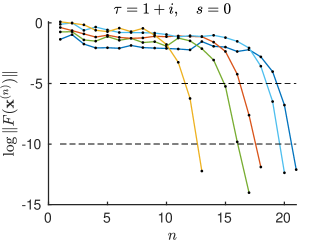
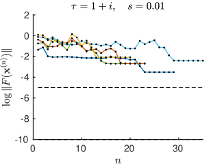
Figure 1. Residual of the function $F$, corresponding to the matrix $\mathbb{B}_{\tau,s}$, in dependence of the $n$-th iteration.

Remark 4.1.

Using Algorithm 1, but with randomly chosen initial vectors, the iterations converge with a frequency of approximately $90\%$ when $\mathbb{B}$ is in the Jacobi locus. We attain the residuals shown in Figure 2 for 1000 different tests for the same matrix $\mathbb{B}_{\tau}$, i.e., 1000 iterations with different randomly chosen initial vectors $X^{(0)},Y^{(0)},Z^{(0)}$ attained $\Delta^{(N)}<10^{-10}$ 896 times. In contrast, none of the tests attained a value below $10^{-5}$ when the considered matrix is $\mathbb{B}_{\tau,s}$ with $s=0.1$.

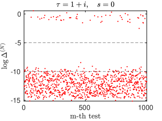
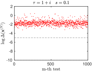
Figure 2. Attained values of $\Delta^{(N)}$ for randomly chosen initial vectors. The left-hand side corresponds to $\mathbb{B}_{\tau,s}$ with $s=0$ and the right-hand side to $s=0.1$.

Let us consider the family of Riemann matrices of the form (32) parametrized by $s\in[-1/2,1/2]$ and $\tau=x+\mathrm{i}$, with $x\in[0,1]$. We expect the Schottky-Igusa form of every $\mathbb{B}_{\tau,s}$ and the residual $\|F(\mathbf{x}^{(N)})\|$ (or its associated minimum singular value) obtained with Algorithm 1 to be within the same order of magnitude. This is indeed what we observe in Figure 3. With this algorithm, we conclude with precision $\delta=10^{-10}$ that the Riemann matrices $\mathbb{B}_{\tau,s}$ with $s\neq 0$ are not in the Jacobi locus, agreeing with the Schottky-Igusa form.

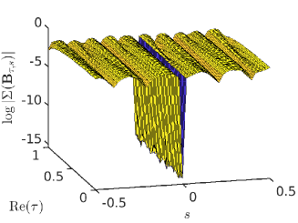
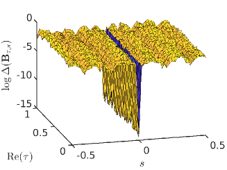
Figure 3. On the left the Schottky-Igusa form and on the right the minimum singular value $\Delta^{(N)}$, both in dependence of the Riemann matrices $\mathbb{B}_{\tau,s}$.

Note that our approach produces numerically essentially the same residuals as the Schottky-Igusa form and is thus of the same practical relevance in deciding whether a matrix is in the Jacobi locus or not with given numerical accuracy. In both cases the input is only the Riemann matrix $\mathbb{B}$, but in the Fay approach an initial iterate for the vectors corresponding to Abel maps for $\mathbb{B}$ in the Jacobi locus.

The matrices $\mathbb{B}_{\tau}$ considered above are in exact form, thus the smallest residual is expected to be zero to machine precision, i.e., approximately $10^{-14}$ with Matlab. However, the smallest $\|F(\mathbf{x}^{(N)})\|$ might be considered as an indicative of the precision of its input matrix $\mathbb{B}$, if this is not in exact form. For example, let us consider the matrices $\mathbb{B}_{\tau,s}=\mathbb{B}_{\tau}+s(M+\mathrm{i}M)$ where $M$ is the symmetric matrix with coefficients $M_{jk}=(j+k)/5$, $\tau=1+\mathrm{i}$ and $s\in[10^{-15},10^{-1}]$ are small perturbations. Thus, $\mathbb{B}_{\tau,s}$ can be seen as the Riemann matrices of the curve (30) with an accuracy of the order $s$. We remove the stopping criterion $\|F(\mathbf{x}^{(N)})\|<\delta$ for this particular example in order to visualize the smallest residual we can achieve with Matlab’s precision.

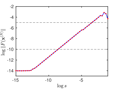
Figure 4. Smallest residuals of period matrices with accuracy $s$.

We can observe in the figure that we attain a residual to machine precision if the matrices are within a precision of approximately $10^{-13}$ and, in particular, the residual is below $\delta=10^{-10}$ if the Riemann matrix is within a precision of the order $\delta$. This is important, since some of the Riemann matrices in higher dimensions are only known numerically.

5. Examples in higher genus

We perform similar tests with matrices in higher genus such as, for example, the period matrices of hyperelliptic curves of arbitrary genus given by [29]. In this paper we only show examples corresponding to the curve

(33) $$\{(x,y)\in\mathbb{C}^{2}\quad|\quad y^{2}=x(x^{2g+1}-1)\},$$

but similar results are obtained with the period matrices of other hyperelliptic curves. The period matrix of (33) is

(34) $$\mathbb{B}_{jk}=1+\frac{1}{\tau_{1}}\sum_{l=1}^{j}\tau_{l}\tau_{k-j+l}\quad\text{for }1\leq j\leq k\leq g,$$

where $\tau_{1}=(-1)^{g}\zeta_{2g+1}^{g^{2}}$ with $\zeta_{m}^{n}=\exp(2\pi\mathrm{i}m/n)$ and

$$\tau_{j+1}=\frac{\tau_{1}}{1+\zeta^{j}_{2g+1}}\left(1-\sum_{l=2}^{j}\zeta_{2g+1}^{g-j+l-1}\tau_{l}\tau_{j-l+2}\right),\quad j=1,...,g-1.$$

We use these matrices for tests up to $g=7$, but we also consider period matrices of non-hyperelliptic curves. For $g=6$ the Fermat curve

(35) $$\{[X:Y:Z]\in\mathbb{P}^{2}\quad|\quad X^{m}+Y^{m}=Z^{m}\},$$

with $m=5$, provides an example. With the numerical approach [16], we get after applying the algorithm [17] the Riemann matrix

ΨRieMat =

  Columns 1 through 4

  -0.3735 + 0.9276i  -0.3574 + 0.4580i  -0.4578 + 0.3092i  -0.2891 + 0.3705i
  -0.3574 + 0.4580i   0.1365 + 1.0006i  -0.0161 + 0.4697i   0.1104 - 0.1415i
  -0.4578 + 0.3092i  -0.0161 + 0.4697i   0.3474 + 1.0079i  -0.2630 - 0.3894i
  -0.2891 + 0.3705i   0.1104 - 0.1415i  -0.2630 - 0.3894i  -0.3152 + 1.1305i
   0.0905 + 0.4390i  -0.4616 + 0.4201i   0.3635 + 0.5382i  -0.3735 - 0.2479i
  -0.4417 - 0.1605i  -0.3313 - 0.3020i   0.2891 - 0.3705i  -0.1725 + 0.0496i

  Columns 5 through 6

   0.0905 + 0.4390i  -0.4417 - 0.1605i
  -0.4616 + 0.4201i  -0.3313 - 0.3020i
   0.3635 + 0.5382i   0.2891 - 0.3705i
  -0.3735 - 0.2479i  -0.1725 + 0.0496i
  -0.4839 + 1.0692i  -0.3796 - 0.0685i
  -0.3796 - 0.0685i  -0.4095 + 0.8023i.

For this curve, we could again compute an Abel map, but we are interested also in perturbations of this Riemann matrix not in the Jacobi locus.
Analogously to (32), we add diagonal perturbations of the form $\mathbb{B}_{s}=\mathbb{B}+s\cdot\mathrm{diag}[2,...,g+1]$ with $s\in[-1/2,1/2]$. As in the previous example, we observe several orders of magnitude of difference between the case $s=0$ and the cases $s\neq 0$. Although a similar behaviour to Figure (4) is to be expected for small values of $s$.

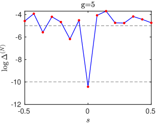
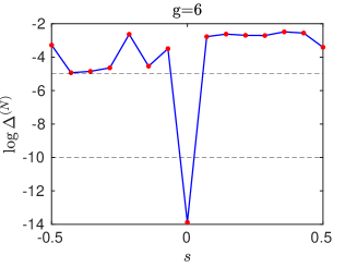
Figure 5. Minimum $\Delta^{(N)}$ obtained for the matrices $\mathbb{B}_{s}\in\mathbb{H}^{g}$ for $g=5$ and $g=6$.

The Fricke-Macbeath curve [18, 24] is a curve of genus 7 with the maximal number $84(g-1)=504$ of automorphisms. It can be defined via the algebraic curve

(36) $$\{(x,y)\in\mathbb{C}^{2}\quad|\quad 1+7yx+21y^{2}x^{2}+35x^{3}y^{3}+28x^{4}y^{4}+2x^{7}+2y^{7}=0\}.$$

After applying the algorithm from [17], the code [16] leads to the Riemann matrix

RieMat =

  Columns 1 through 4

   0.3967 + 1.0211i   0.0615 - 0.1322i   0.0000 - 0.0000i   0.4609 + 0.2609i
   0.0615 - 0.1322i   0.3967 + 1.0211i  -0.3553 + 0.5828i   0.3386 - 0.1933i
   0.0000 - 0.0000i  -0.3553 + 0.5828i   0.2894 + 1.1656i   0.0905 + 0.2450i
   0.4609 + 0.2609i   0.3386 - 0.1933i   0.0905 + 0.2450i   0.3967 + 1.0211i
  -0.3553 + 0.5828i  -0.4776 + 0.1287i  -0.4776 + 0.1287i  -0.4776 + 0.1287i
  -0.1838 - 0.3219i  -0.2743 - 0.5669i   0.3871 - 0.3736i   0.0167 - 0.3895i
   0.3386 - 0.1933i   0.3386 - 0.1933i  -0.1223 - 0.4541i   0.0615 - 0.1322i

  Columns 5 through 7

  -0.3553 + 0.5828i  -0.1838 - 0.3219i   0.3386 - 0.1933i
  -0.4776 + 0.1287i  -0.2743 - 0.5669i   0.3386 - 0.1933i
  -0.4776 + 0.1287i   0.3871 - 0.3736i  -0.1223 - 0.4541i
  -0.4776 + 0.1287i   0.0167 - 0.3895i   0.0615 - 0.1322i
   0.2894 + 1.1656i  -0.1671 - 0.7115i   0.0905 + 0.2450i
  -0.1671 - 0.7115i   0.4414 + 1.2784i  -0.3386 + 0.1933i
   0.0905 + 0.2450i  -0.3386 + 0.1933i   0.3967 + 1.0211i.

The accuracy of this matrix is estimated to be of the order of $10^{-10}$.

Fast convergence when $\mathbf{x}^{(n)}$ falls into a basin of attraction is still observed in higher genus. For example, let us observe the convergence of the residual of $F$ corresponding to the period matrix of Fermat curve for $g=6$ and the period matrix of the Fricke curve for $g=7$. The dimension of the domain of $F$ increases linearly with $g$, thus it might take more steps for the iteration to find a basin of attraction, but when it does, fast convergence is assured.

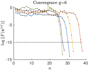
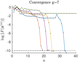
Figure 6. Residual of the function $F$ in dependence of the $n$-th iteration.

It is worth mentioning that the convergence is slower if the matrix $\mathbb{B}$ corresponds to the hyperelliptic example, as we can see in Figure 7 for the curve (33) with $g=6$ and $g=7$. This might be due to the extra symmetries in their matrix elements, which makes the convergence slower. However, these are just special cases amongst all the possible matrices in $\mathbb{H}^{g}$.

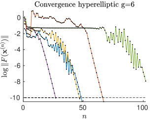
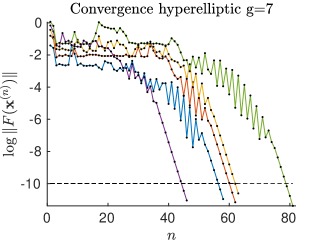
Figure 7. Residual of the function $F$ in dependence of the $n$-th iteration.

The computation per step becomes more expensive as $g$ increases since the number of summands in the approximation of every theta function is $(2\mathcal{N}_{\delta}+1)^{g}$. Besides that, we need to compute $2^{g}$ even and $6$ odd theta functions in each step. This increases the computational time of the whole algorithm. As a reference, the total time of the tests for the period matrices of non-hyperelliptic curves with $g=4,5,6$ presented in Figures 1 and 6 consisting of $5$ iterative processes are

$g$	time
4	6 s
6	28 min
7	19 h

.

However, since it suffices finding only one zero, the computations can also be terminated as soon as we find a vector with $\|F(\mathbf{x}^{(n)})\|<\delta$, thus reducing these times. On the other hand, the total computational time of the five iterative processes for the period matrices of hyperelliptic curves are

$g$	time
4	14 s
5	98 s
6	56 min
7	30 h

6. Outlook

In this paper, we have shown how the Fay identity can be used to identify the Jacobi locus for small genera in a computational context. Concretely, the Fay identity in the form (5) is considered for a given Riemann matrix $\mathbb{B}$ and its fulfilment is probed by using a Newton iteration. Four components of the vectors $X$, $Y$ and $Z$ are fixed in order to avoid convergence to a trivial solution where two or more of the vectors coincide. This leads to an iteration to find the zeros of a function $F$ depending on the vector $\mathbf{x}$ with $3g-4$ complex components. The starting point for the iteration is the choice (28).

The approach uses a finite precision $\delta$, and the answer to whether a matrix is in the Jacobi locus is thus given with this accuracy. In this paper, we have only studied the case of so-called double precision leading in practice to a $\delta\sim 10^{-12}$. However, the code is set up in a way that inclusion of multi-precision packages is straightforward allowing essentially arbitrary precision.

We have considered in this paper examples up to $g=7$. This limit is imposed by the size of memory on the used standard computers for the computation of the theta functions. Since the algorithm [17] allows the computation of theta functions and their derivatives with a truncation parameter $\mathcal{N}_{\delta}=5$ in double precision, these computations are very efficient. In order to take advantage of Matlab’s vectorization algorithms, the exponentials of the theta function (13) are stored in one array with $11^{g}$ components. If one wants to go to higher values of $g$, the memory limitations can be avoided by not storing these values and applying loops to compute them. The Jacobian matrix in (25) is of complex dimension $2^{g}\times(3g-4)$, but its computation is also fully parallelizable. It will be the subject of further research which genera can be reasonably studied with this approach.

We note that the algorithm produces as a by-product three vectors being linear combinations of the Abel maps of four points if the Riemann matrix is identified to be in the Jacobi locus. The resulting vectors are just auxiliary to test whether the Fay identity is satisfied. It is an interesting question whether they can be used to identify the defining algebraic curves in a similar way as in [1].

Appendix A Algorithm

Algorithm 1 Algorithm to find trisecant points

procedure Trisecant($\mathbb{B}$)$\triangleright$ Find one trisecant in the Kummer variety of $X_{\mathbb{B}}$

     $\mathbb{B}\leftarrow\mathtt{siegeltrans}(\mathbb{B})$ $\triangleright$ Find Siegel’s transform of $\mathbb{B}$

     $\delta\leftarrow 10^{-10}$ $\triangleright$ Set precision $\delta$

     $\ell\leftarrow 0.1$

     $\Delta\ell\leftarrow 0.1$

     $\mathtt{max\_iter}\leftarrow 100$ $\triangleright$ Set maximum number of iterations

     $\Delta_{N}\leftarrow[\quad]$

     while $\ell\geq 0.5$ do

         $X\leftarrow\ell/2\left(e_{g-2}+\mathbb{B}e_{g-2}\right)$

         $Y\leftarrow\ell/2\left(e_{g-1}+\mathbb{B}e_{g-1}\right)$

         $Z\leftarrow\ell/2\left(e_{g}+\mathbb{B}e_{g}\right)$

         $\mathbf{x}\leftarrow[X(3:g);Y(2:g);Z(2:g)]$ $\triangleright$ Initial vector

         $V\leftarrow[X(1:2);Y(1);Z(1)]$ $\triangleright$ Fixed components $X_{1}$, $X_{2}$, $Y_{1}$, $Z_{1}$

         $[F,JF,\mathbf{x},\mathrm{res},\Delta]\leftarrow\mathtt{fay}(\mathbf{x},V,\mathbb{B})$

         $\boldsymbol{\varepsilon}\leftarrow-JF\backslash F$

         $\mathtt{iter}\leftarrow 1$

         while $\|\boldsymbol{\varepsilon}\|<\delta$ do $\triangleright$ Newton’s iteration

              $\mathbf{x}\leftarrow\mathbf{x}+\boldsymbol{\varepsilon}$

              $[F,JF,\mathbf{x},\mathrm{res},\Delta]\leftarrow\mathtt{fay}(\mathbf{x},W,\mathbb{B})$

              $\boldsymbol{\varepsilon}\leftarrow-JF\backslash F$

              if $\mathrm{res}<\delta$ or $\mathtt{iter}>\mathtt{max\_iter}$ then

                  End Newton’s iteration

              end if

              $\mathtt{iter}\leftarrow\mathtt{iter}+1$

         end while

         $\Delta_{N}\leftarrow[\Delta_{N},\Delta]$ $\triangleright$ Store the smallest $\Delta$ for each $\ell$

         $\Delta_{\min}\leftarrow\min(\Delta_{N})$

         if $\Delta_{\min}<\delta$ then

              End algorithm

         end if

         $\ell\leftarrow\ell+\Delta\ell$

     end while

     return $\mathrm{res}$, $\Delta_{\min}$

end procedure

The following is the routine computing the function $F:W\subset\mathbb{C}^{3g-4}\to\mathbb{C}^{2^{g}}$, where the fixed components $X_{1},X_{2},Y_{1},Z_{1}$ are entered as parameters.

Algorithm 2 Algorithm to compute the function $F$

procedure fay($\mathbf{x},V,\mathbb{B}$)

     $X\leftarrow[V(1:2);\mathbf{x}(1:g-2)]$

     $Y\leftarrow[V(3);\mathbf{x}(g-1:2g-3)]$

     $Z\leftarrow[V(4);\mathbf{x}(2g-2:2g-4)]$

     $X\leftarrow[[X]]$ $\triangleright$ Keep $X,Y,Z$ in the fundamental domain

     $Y\leftarrow[[Y]]$

     $Z\leftarrow[[Z]]$

     $\mathbf{x}\leftarrow[X(3:g);Y(2:g);Z(2:g)]$

     $[\lambda_{1},\nabla_{Y}\lambda_{1},\nabla_{Z}\lambda_{1}]\leftarrow\mathtt{lambdafun}(Y,Z,\mathbb{B})$

     $[\lambda_{2},\nabla_{Z}\lambda_{2},\nabla_{X}\lambda_{2}]\leftarrow\mathtt{lambdafun}(Z,X,\mathbb{B})$

     $[\lambda_{2},\nabla_{X}\lambda_{3},\nabla_{Y}\lambda_{3}]\leftarrow\mathtt{lambdafun}(X,Y,\mathbb{B})$

     $[KX,JKX]\leftarrow\mathtt{kummer}(X,\mathbb{B})$

     $[KY,JKY]\leftarrow\mathtt{kummer}(Y,\mathbb{B})$

     $[KZ,JKZ]\leftarrow\mathtt{kummer}(Z,\mathbb{B})$

     $F\leftarrow KX+\frac{\lambda_{2}}{\lambda_{1}}KY+\frac{\lambda_{3}}{\lambda_{1}}KZ$

     $J_{X}F\leftarrow JKX+\frac{1}{\lambda_{1}}KY*\nabla_{X}\lambda_{2}+\frac{1}{\lambda_{1}}KZ*\nabla_{X}\lambda_{3}$

     $J_{Y}F\leftarrow\frac{\lambda_{2}}{\lambda_{1}}JKY+\frac{1}{\lambda_{1}}KZ*\nabla_{Y}\lambda_{3}-\frac{1}{(\lambda_{1})^{2}}\left[\lambda_{2}KY+\lambda_{3}KZ\right]*\nabla_{Y}\lambda_{1}$

     $J_{Z}F\leftarrow\frac{1}{\lambda_{1}}KY*\nabla_{Z}\lambda_{2}+\frac{\lambda_{3}}{\lambda_{1}}JKZ-\frac{1}{(\lambda_{1})^{2}}\left[\lambda_{2}KY+\lambda_{3}KZ\right]*\nabla_{Z}\lambda_{1}$

     $JF=[J_{X}F,J_{Y}F,J_{Z}F]$

     $JF(:,[1,2,g+1,2g+1])\leftarrow[\quad]$ $\triangleright$ Deleting columns corresponding to $X_{1},X_{2},Y_{1},Z_{1}$

     $\mathrm{res}\leftarrow\|F\|$ $\triangleright$ Residual of $F$

     $\Delta\leftarrow\mathrm{min}\left(\mathrm{svd}(KX,KY,KZ)\right)$ $\triangleright$ Linear dependence of $KX$ $KY$, $KZ$

     return $F,JF,\mathbf{x},\mathrm{res},\Delta$

end procedure

Where $\mathtt{kummer}(X,\mathbb{B})$ is the routine computing $\vec{\Theta}(X)$ (which is expressed as a column vector) and its Jacobian matrix $J\vec{\Theta}(X)$. The operation $*$ is the matrix multiplication.

Algorithm 3 Algorithm to compute the Kummer map

procedure kummer($X,\mathbb{B}$)

     for $I=1:2^{g}$ do

         Set characteristic $\epsilon_{I}$ $\triangleright$ $\epsilon_{I}\in\{0,1\}^{g}$ in column vector form

         $factor\leftarrow\exp\left(\frac{1}{2}\pi\mathrm{i}\langle\epsilon_{I},\mathbb{B}\epsilon_{I}\rangle+2\pi\mathrm{i}\langle\epsilon_{I},X\rangle\right)$

         $[t,\nabla t]\leftarrow\texttt{thetagrad}(2X+\mathbb{B}\epsilon_{I},2\mathbb{B},0)$

         $K(I)\leftarrow factor\cdot t$

         $JK(I,:)\leftarrow 2\cdot factor\cdot(\nabla t+t\cdot\epsilon_{I}^{T})$

     end for

     return $K,JK$

end procedure

The routine $\mathtt{thetagrad}(X,\mathbb{B},C)$ computes the multidimensional theta function $\Theta[C](X,\mathbb{B})$ defined in (13) with characteristic $C=\big{[}\begin{smallmatrix}\mathrm{p}\\ \mathrm{q}\end{smallmatrix}\big{]}$, as well as its gradient $\nabla\Theta[C](X,\mathbb{B})$ (which is expressed as a row vector) through (24). We used the relation (14) to compute the even theta functions more efficiently in terms of the zero-characteristic theta function, since in practice we enter the array containing $\langle\mathrm{N},\mathbb{B}\mathrm{N}\rangle$ as an input, rather than computing $\langle(\mathrm{N}+\epsilon_{I}/2),\mathbb{B}(\mathrm{N}+\epsilon_{I}/2)\rangle$ for every $\epsilon_{I}\in Z^{g}/2\mathbb{Z}^{g}$, which would take up more memory space. Finally, the routine to compute the function $\lambda(a,b):=\Theta^{*}(a+b,\mathbb{B})\Theta^{*}(a-b,\mathbb{B})$ with and odd characteristic $2\delta_{o}\in\mathbb{Z}^{2g}/2\mathbb{Z}^{2g}$, as well as its gradients $\nabla_{a}\lambda(a,b)$, $\nabla_{b}\lambda(a,b)$ is the following:

Algorithm 4 Algorithm to compute the lambda coefficients

procedure lambdafun($a,b,\mathbb{B}$)

     $\delta_{o}\leftarrow[e_{1}/2;e_{1}/2]$ $\triangleright$ Default odd characteristic

     $[t_{p},\nabla t_{p}]\leftarrow\mathtt{thetagrad}(a-b,\mathbb{B},\delta_{o})$

     $[t_{m},\nabla t_{m}]\leftarrow\mathtt{thetagrad}(a+b,\mathbb{B},\delta_{o})$

     $\lambda\leftarrow t_{p}\cdot t_{m}$

     $\nabla_{a}\lambda\leftarrow t_{m}\nabla t_{p}+t_{p}\nabla t_{m}$

     $\nabla_{b}\lambda\leftarrow t_{m}\nabla t_{p}-t_{p}\nabla t_{m}$

     return $\lambda,\nabla_{a}\lambda,\nabla_{b}\lambda$

end procedure

As before, since we use the same odd characteristic throughout the whole algorithm, we enter $\langle(\mathrm{N}+e_{1}/2),\mathbb{B}(\mathrm{N}+e_{1}/2)\rangle$ as an input in the computation of the odd theta function $\Theta^{*}(\mathrm{z},\mathbb{B})$ and its gradient.

References

- [1] D. Agostini, T. Celik, D. Eken. Numerical Reconstruction of Curves from their Jacobians, Proceedings of the 18th Conference on Arithmetic, Geometry, Cryptography, and Coding Theory, AMS book series Contemporary Mathematics (2021).
- [2] D. Agostini and L. Chua. Computing theta functions with Julia. Journal of Software for Algebra and Geometry, Vol. 11 (2021), 41?51.
- [3] E. Arbarello and C. De Concini. On a set of equations characterizing Riemann matrices. Ann. of Math., 120(1), 119-140 (1984).
- [4] E.D. Belokolos, A.I. Bobenko, V.Z. Enolskii, A.R. Its, V.B. Matveev. Algebro-geometric approach to nonlinear integrable equations. Springer, Berlin (1994)
- [5] C. Birkenhake and H. Lange. Complex Abelian Varieties. Grundlagen der Mathematischen Wissenschaften 302. Springer Verlag, Berlin (2004)
- [6] H. W. Braden and T.P. Northover. Bring’s Curve: its Period Matrix and the Vector of Riemann Constants, SIGMA 8, 065, 2012
- [7] A.I. Bobenko and C. Klein (ed.). Computational Approach to Riemann Surfaces, Lect. Notes Math. 2013 (2011)
- [8] L. Chua, M. Kummer and B. Sturmfels. Schottky Algorithms: Classical meets Tropical, Mathematics of computation, 88, 2541-2558, (2019)
- [9] B. Deconinck and M. van Hoeij. Computing Riemann matrices of algebraic curves. Physica D, 152-153, 28 (2001)
- [10] B. Deconinck, M. Heil, A. Bobenko, M. van Hoeij, M. Schmies. Computing Riemann theta functions. Mathematics of Computation, 73, 1417–1442 (2004)
- [11] R. Donagi. Big Schottky. Invent. Math., 89(3), 569-599, 1987.
- [12] B.A. Dubrovin. Theta functions and non-linear equations, Usp. Mat. Nauk 36, No. 2, 11–80 (1981) (English translation: Russ. Math. Surv. 36, No. 2, 11–92 (1981)).
- [13] H.M. Farkas, S. Grushevsky, and R. Salvati Manni. An explicit solution to the weak Schottky problem, Algebr. Geom. 8:3 (2021), 358-373
- [14] H.M. Farkas and I. Kra. Riemann surfaces, Graduate Texts in Mathematics 71, Springer-Verlag, Berlin - Heidelberg - New York (1980).
- [15] J.D. Fay. Theta functions on Riemann surfaces. Lect. Notes in Math., 352, Springer (1973)
- [16] J. Frauendiener and C. Klein. Computational approach to compact Riemann surfaces, Nonlinearity 30(1), 138 (2016).
- [17] J. Frauendiener, C. Jaber and C. Klein. Efficient computation of multidimensional theta functions, J. Geom. Phys. 141, 147-158 (2019)
- [18] R. Fricke. Über eine einfache Gruppe von 504 Operationen, Mathematische Annalen, 52 (23): 321–339, (1899)
- [19] S. Grushevsky. The Schottky problem, Current developments in algebraic geometry, Math. Sci. Res. Inst. Publ., 59, Cambridge Univ. Press, 2012, pp. 129-164.
- [20] S. Grushevsky and M. Möller. Explicit formulas for infinitely many Shimura curves in genus 4, ASIAN J. MATH. 22(2), 0381-0390, (2018)
- [21] J. Igusa. On the irreducibility of Schottky’s divisor, J. Fac. Sci. Univ. Tokyo Sect. IA Math. 28 (1981) 531-545.
- [22] I. Krichever. Characterizing Jacobians via trisecants of the Kummer variety. Ann. of Math. (2), 172(1), 485-516, 2010.
- [23] A.K. Lenstra, H.W. Lenstra, Jr., L. Lovász. Factoring polynomials with rational coefficients. Math. Ann, 261, 515–534 (1982).
- [24] A. Macbeath. On a curve of genus 7, Proceedings of the London Mathematical Society 15, 527–542, (1965)
- [25] H. Minkowski. Über die positiven quadratischen Formen und über kettenbruchähnliche Algorithmen, J. Reine und Angewandte Math., 107, 278-297.
- [26] H. Minkowski. Gesammelte Abhandlungen 1, pp. 145-148, 153-156, 217-218 (Leipzig-Berlin: Teubner 1911).
- [27] D. Mumford. Tata lectures on theta. II, volume 29 of Progress in Mathematics. (Birkhäuser, Boston, MA, 1983)
- [28] H. Rauch and H. Farkas. Theta functions with applications to Riemann surfaces. The Williams & Wilkins Co., Baltimore, Md., 1974.
- [29] B. Schindler. Period Matrices of Hyperelliptic Curves. Manuscr. Math. 78, 369-380 (1993)
- [30] F. Schottky. Zur Theorie der Abelschen Funktionen von vier Variabeln, J. reine angewandte Mathematik 102 (1888) 304-352.
- [31] T. Shiota. Characterization of Jacobian varieties in terms of soliton equations. Invent. Math., 83(2), 333-382 (1986)
- [32] C.L. Siegel. Topics in complex function theory. Vol. III. John Wiley & Sons, Inc., New York, 1989.
- [33] C. Swierczewski and B. Deconinck. Computing Riemann theta functions in Sage with applications, Mathematics and Computers in Simulation, ISSN 0378-4754, http://dx.doi.org/10.1016/j.matcom.2013.04.018 (2013).
- [34] I. A. Taimanov. Secants of Abelian varieties, theta functions, and soliton equations, Russian Mathematical Surveys, 1997, 52:1, 147-218
- [35] G. Welters. A criterion for Jacobi varieties. Ann. of Math., 120: 497-504, 1984.