Manifold Learning by Mixture Models of VAEs for Inverse Problems

Abstract

Representing a manifold of very high-dimensional data with generative models has been shown to be computationally efficient in practice. However, this requires that the data manifold admits a global parameterization. In order to represent manifolds of arbitrary topology, we propose to learn a mixture model of variational autoencoders. Here, every encoder-decoder pair represents one chart of a manifold. We propose a loss function for maximum likelihood estimation of the model weights and choose an architecture that provides us the analytical expression of the charts and of their inverses. Once the manifold is learned, we use it for solving inverse problems by minimizing a data fidelity term restricted to the learned manifold. To solve the arising minimization problem we propose a Riemannian gradient descent algorithm on the learned manifold. We demonstrate the performance of our method for low-dimensional toy examples as well as for deblurring and electrical impedance tomography on certain image manifolds.

1 Introduction

Manifold learning.

The treatment of high-dimensional data is often computationally costly and numerically unstable. Therefore, in many applications, it is important to find a low-dimensional representation of high-dimensional datasets. Classical methods, like the principal component analysis (PCA) [75], assume that the data is contained in a low-dimensional subspace. However, for complex datasets this assumption appears to be too restrictive, particularly when working with image datasets. Therefore, recent methods rely on the so-called manifold hypothesis [16], stating that even complex and high-dimensional datasets are contained in a low-dimensional manifold. Based on this hypothesis, in recent years, many successful approaches have been based on generative models, able to represent high dimensional data in $\mathbb{R}^{n}$ by a generator $D\colon\mathbb{R}^{d}\to\mathbb{R}^{n}$ with $d\ll n$: these include generative adversarial networks (GANs) [40], variational autoencoders (VAEs) [58], injective flows [63] and score-based diffusion models [85, 50]. For a survey on older approaches to manifold learning, the reader is referred to [68, 55] and to the references therein.

Learning manifolds with multiple charts.

Under the assumption that $D$ is injective, the set of generated points $\{D(z)\mathrel{\mathop{\ordinarycolon}}z\in\mathbb{R}^{d}\}$ forms a manifold that approximates the training set. However, this requires that the data manifold admits a global parameterization. In particular, it must not be disconnected or contain holes. In order to model disconnected manifolds, the authors of [76] propose to model the latent space of a VAE by a Gaussian mixture model. Similarly, the authors of [31, 71, 78] propose latent distributions defined on Riemannian manifolds for representing general topologies. In [70], the manifold is embedded into a higher-dimensional space, in the spirit of Whitney embedding theorem. However, these approaches have the drawback that the topology of the manifold has to be known a priori, which is usually not the case in practice.

Here, we focus on the representation of the data manifold by several charts. A chart provides a parameterization of an open subset from the manifold by defining a mapping from the manifold into a Euclidean space. Then, the manifold is represented by the collection of all of these charts, which is called atlas. For finding these charts, the authors of [29, 38, 77, 83] propose the use of clustering algorithms. By default, these methods do not provide an explicit formulation of the resulting charts. As a remedy, the authors of [77] use linear embeddings. The authors of [83] propose to learn for each chart again a generative model. However, these approaches often require a large number of charts and are limited to relatively low data dimensions. The idea of representing the charts by generative models is further elaborated in [61, 62, 81]. Here, the authors proposes to train at the same time several (non-variational) autoencoders and a classification network that decides for each point to which chart it belongs. In contrast to the clustering-based algorithms, the computational effort scales well for large data dimensions. On the other hand, the numerical examples in the corresponding papers show that the approach already has difficulties to approximate small toy examples like a torus.

In this paper, we propose to approximate the data manifold by a mixture model of VAEs. Using Bayes theorem and the ELBO approximation of the likelihood term we derive a loss function for maximum likelihood estimation of the model weights. Mixture models of generative models for modelling disconnected datasets were already considered in [13, 51, 65, 86, 88]. However, they are trained in a different way and to the best of our knowledge none of those is used for manifold learning.

Inverse Problems on Manifolds.

Many problems in applied mathematics and image processing can be formulated as inverse problems. Here, we consider an observation $y$ which is generated by

$$y=\mathcal{G}(x)+\eta,$$ (1)

where $\mathcal{G}\colon\mathbb{R}^{n}\to\mathbb{R}^{m}$ is an ill-posed or ill-conditioned, possibly nonlinear, forward operator and $\eta$ represents additive noise. Reconstructing the input $x$ directly from the observation $y$ is usually not possible due to the ill-posed operator and the high dimension of the problem. As a remedy, the incorporation of prior knowledge is required. This is usually achieved by using regularization theory, namely, by minimizing the sum of a data fidelity term $F(x)$ and a regularizer $R(x)$, where $F$ describes the fit of $x$ to $y$ and $R$ incorporates the prior knowledge. With the success of deep learning, data-driven regularizers became popular [6, 9, 41, 49, 67].

In this paper, we consider a regularizer which constraints the reconstruction $x$ to a learned data manifold $\mathcal{M}$. More precisely, we consider the optimization problem

$$\hat{x}=\operatorname*{arg\,min}_{x}F(x)\quad\text{subject to $x\in\mathcal{M}$,}$$

where $F(x)=\frac{1}{2}\|\mathcal{G}(x)-y\|^{2}$ is a data-fidelity term. This corresponds to the regularizer $R(x)$ which is zero for $x\in\mathcal{M}$ and infinity otherwise. When the manifold admits a global parameterization given by one single generator $D$, the authors of [4, 23, 33, 39] propose to reformulate the problem as $\hat{x}=\hat{z}$, where $\hat{z}=\operatorname*{arg\,min}_{z}F(D(x))$. Since this is an unconstrained problem, it can be solved by gradient based methods. However, since we consider manifolds represented by several charts, this reformulation cannot be applied. As a remedy, we propose to use a Riemannian gradient descent scheme. In particular, we derive the Riemannian gradient using the decoders and encoders of our manifold and propose two suitable retractions for applying a descent step into the gradient direction.

To emphasize the advantage of using multiple generators, we demonstrate the performance of our method on numerical examples. We first consider some two- and three-dimensional toy examples. Finally, we apply our method to deblurring and to electrical impedance tomography (EIT), a nonlinear inverse problem consisting in the reconstruction of the leading coefficient of a second order elliptic PDE from the knowledge of the boundary values of its solutions [27]. The code of the numerical examples is available online.

Outline.

The paper is organized as follows. In Section 2, we revisit VAEs and fix the corresponding notations. Afterwards, in Section 3, we introduce mixture models of VAEs for learning embedded manifolds of arbitrary dimensions and topologies. Here, we focus particularly on the derivation of the loss function and of the architecture, which allows us to access the charts and their inverses. For minimizing functions defined on the learned manifold, we propose a Riemannian gradient descent scheme in Section 4. We provide numerical toy examples for one and two dimensional manifolds in Section 5. In Section 6, we discuss the applications to deblurring and to electrical impedance tomography. Conclusions are drawn in Section 7.

2 Variational Autoencoders for Manifold Learning

In this paper, we assume that we are given data points $x_{1},\dots,x_{N}\in\mathbb{R}^{n}$ for a large dimension $n$. In order to reduce the computational effort and to regularize inverse problems, we assume that these data-points are located in a lower-dimensional manifold. We aim to learn the underlying manifold from the data points $x_{1},\dots,x_{N}$ with a VAE [58, 59].

A VAE aims to approximate the underlying high-dimensional probability distribution $P_{X}$ of the random variable $X$ with a lower-dimensional latent random variable $Z\sim P_{Z}$ on $\mathbb{R}^{d}$ with $d<n$, by using the data points $x_{1},\dots,x_{N}$. To this end, we define a decoder $D\colon\mathbb{R}^{d}\to\mathbb{R}^{n}$ and an encoder $E\colon\mathbb{R}^{n}\to\mathbb{R}^{d}$. The decoder approximates $P_{X}$ by the distribution $P_{\tilde{X}}$ of a random variable $\tilde{X}\coloneqq D(Z)+\eta$, where $\eta\sim\mathcal{N}(0,\sigma_{x}^{2}I_{n})$. Vice versa, the encoder approximates $P_{Z}$ from $P_{X}$ by the distribution $P_{\tilde{Z}}$ of the random variable $\tilde{Z}\coloneqq E(X)+\xi$ with $\xi\sim\mathcal{N}(0,\sigma_{z}^{2}I_{d})$. Now, decoder and encoder are trained such that we have $P_{X}\approx P_{\tilde{X}}$ and $P_{Z}\approx P_{\tilde{Z}}$. To this end, we aim to maximize the log-likelihood function $\ell(\theta)=\sum_{i=1}^{N}\log(p_{\tilde{X}}(x_{i})),$ where $\theta$ denotes the parameters $D$ and $E$ depend upon.

The log-density $\log(p_{\tilde{X}}(x))$ induced by the model is called the evidence. However, for VAEs the computation of the evidence is intractable. Therefore, the authors of [58] suggest to approximate the evidence by Jensens’s inequality as

$$\log(p_{\tilde{X}}(x)) =\log\Big{(}\int_{\mathbb{R}^{d}}p_{Z,\tilde{X}}(z,x)\,\mathrm{d}z\Big{)}$$ (2)

$$=\log\Big{(}\int_{\mathbb{R}^{d}}\frac{p_{Z,\tilde{X}}(z,x)}{p_{\tilde{Z}|X=x}(z)}p_{\tilde{Z}|X=x}(z)\,\mathrm{d}z\Big{)}$$ (3)

$$\geq\int_{\mathbb{R}^{d}}\log\Big{(}\frac{p_{Z,\tilde{X}}(z,x)}{p_{\tilde{Z}|X=x}(z)}\Big{)}p_{\tilde{Z}|X=x}(z)\,\mathrm{d}z\Big{)}$$ (4)

$$=\mathbb{E}_{z\sim P_{\tilde{Z}|X=x}}\Big{[}\log\Big{(}\frac{p_{Z}(z)p_{\tilde{X}|Z=z}(x)}{p_{\tilde{Z}|X=x}(z)}\Big{)}\Big{]}$$ (5)

$$=\mathbb{E}_{z\sim P_{\tilde{Z}|X=x}}[\log(p_{Z}(z))+\log(p_{\tilde{X}|Z=z}(x))-\log(p_{\tilde{Z}|X=x}(z))].$$ (6)

Accordingly to the definition of $\tilde{Z}$ and $\tilde{X}$, we have that $p_{\tilde{X}|Z=z}(x)=\mathcal{N}(x;D(z),\sigma_{x}^{2}I_{n})$ and $p_{\tilde{Z}|X=x}(z)=\mathcal{N}(z;E(x),\sigma_{z}^{2}I_{d})$. Thus, the above formula is, up to a constant, equal to

$$\mathbb{E}_{z\sim P_{\tilde{Z}|X=x}}[\log(p_{Z}(z))-\tfrac{1}{2\sigma_{x}^{2}}\|x-D(z)\|^{2}-\log(\mathcal{N}(z;E(x),\sigma_{z}^{2}I_{d}))].$$ (7)

Considering the substitution $\xi=(z-E(x))/\sigma_{z}$, we obtain

$$\mathbb{E}_{\xi\sim\mathcal{N}(0,I_{d})}[\log(p_{Z}(E(x)+\sigma_{z}\xi))-\tfrac{1}{2\sigma_{x}^{2}}\|D(E(x)+\sigma_{z}\xi)-x\|^{2}-\log(\mathcal{N}(\xi;0,I_{d}))].$$ (8)

Note that also the last summand does not depend on $D$ and $E$. Thus, we obtain, up to a constant, the evidence lower bound (ELBO) given by

$$\mathrm{ELBO}(x|\theta)\coloneqq\mathbb{E}_{\xi\sim\mathcal{N}(0,I_{d})}[\log(p_{Z}(E(x)+\sigma_{z}\xi))-\tfrac{1}{2\sigma_{x}^{2}}\|D(E(x)+\sigma_{z}\xi)-x\|^{2}].$$ (9)

Finally, a VAE is trained by minimizing the loss function which sums up the negative ELBO values of all data points, i.e.,

$$\mathcal{L}_{\mathrm{VAE}}(\theta)=-\sum_{i=1}^{N}\mathrm{ELBO}(x_{i}|\theta).$$

Learned Latent Space.

To improve the expressiveness of our VAEs, we use a latent space learned by a normalizing flow. This was first proposed in [79] and further used, e.g., in [30]. Here, we employ the specific loss function from [43, 44] for training the arising model. More precisely, we choose the latent distribution

$$P_{Z}={\mathcal{T}}_{\#}P_{\Xi},$$

where $\mathcal{T}\colon\mathbb{R}^{d}\to\mathbb{R}^{d}$ is an invertible neural network, called normalizing flow. In this way, $P_{Z}$ is the push-forward of a fixed (known) distribution $P_{\Xi}$. Then, the density $p_{Z}$ is given by

$$p_{Z}(z)=p_{\Xi}(\mathcal{T}^{-1}(z))|\mathrm{det}(\nabla\mathcal{T}^{-1}(z))|.$$

The parameters of $\mathcal{T}$ are considered as trainable parameters. Then, the ELBO reads as

$$\mathrm{ELBO}(x|\theta) \coloneqq\mathbb{E}_{\xi\sim\mathcal{N}(0,I_{d})}[\log(p_{\Xi}(\mathcal{T}^{-1}(E(x)+\sigma_{z}\xi)))$$ (10)

$$+\log(|\mathrm{det}(\nabla\mathcal{T}^{-1}(E(x)+\sigma_{z}\xi))|)-\tfrac{1}{2\sigma_{x}^{2}}\|D(E(x)+\sigma_{z}\xi)-x\|^{2}],$$

where $\theta$ are the parameters of the decoder, the encoder and of the normalizing flow $\mathcal{T}$.

In the literature, there exist several invertible neural network architectures based on coupling blocks [32, 57], residual networks [15, 24, 48], ODE representations [25, 42, 74] and autoregressive flows [52]. In our numerics, we use the coupling-based architecture from [8].

Manifold Learning with VAEs.

In order to obtain a lower-dimensional representation of the data points, some papers propose to approximate the data-manifold by $\mathcal{M}\coloneqq\{D(z)\mathrel{\mathop{\ordinarycolon}}z\in\mathbb{R}^{d}\}$, see e.g. [4, 23, 33, 39]. However, this is only possible if the data-manifold admits a global parameterization, i.e., it can be approximated by one generating function. This assumption is often violated in practice. As a toy example, consider the one-dimensional manifold embedded in $\mathbb{R}^{2}$ that consists of two circles, see Figure 1(a). This manifold is disconnected and contains “holes”. Consequently, the topologies of the manifold and of the latent space $\mathbb{R}$ do not coincide, so that the manifold cannot be approximated by a VAE. Indeed, this can be verified numerically. When we learn a VAE for approximating samples from this manifold, we observe that the two (generated) circles are not closed and that both components are connected, see Figure 1(b). As a remedy, in the next section, we propose the use of multiple generators to resolve this problem, see Figure 1(c).

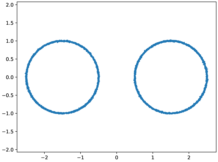
(a) Noisy samples from the manifold.

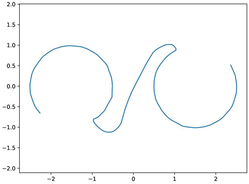
(b) Approximation with one chart.

(c) Approximation with four charts.

Figure 1: Example of a one-dimensional manifold that admits no global parameterization.

3 Chart Learning by Mixtures of VAEs

In order to approximate (embedded) manifolds with arbitrary (unknown) topology, we propose to learn several local parameterizations of the manifold instead of a global one. To this end, we propose to use mixture models of VAEs.

Embedded Manifolds.

A subset $\mathcal{M}\subseteq\mathbb{R}^{n}$ is called a $d$-dimensional embedded differentiable manifold if there exists a family $(U_{k},\varphi_{k})_{k\in I}$ of relatively open sets $U_{k}\subseteq\mathcal{M}$ with $\bigcup_{k\in I}U_{k}=\mathcal{M}$ and mappings $\varphi_{k}\colon U_{k}\to\mathbb{R}^{d}$ such that it holds for every $k,l\in I$ that

• $\varphi_{k}$ is a homeomorphism between $U_{k}$ and $\varphi_{k}(U_{k})$;

• the inverse $\varphi_{k}^{-1}\colon\varphi_{k}(U_{k})\to U_{k}$ is continuously differentiable;

• the transition maps $\varphi_{k}\circ\varphi_{l}^{-1}\colon\varphi_{l}(U_{k}\cap U_{l})\to\varphi_{k}(U_{k}\cap U_{l})$ are continously differentiable;

• and the Jacobian $\nabla\varphi_{k}^{-1}(x)$ of $\varphi_{k}^{-1}$ at $x$ has full column-rank for any $x\in\varphi_{k}(U_{k})$.

We call the mappings $\varphi_{k}$ charts and the family $(U_{k},\varphi_{k})_{k\in I}$ an atlas. With an abuse of notation, we sometimes also call the set $U_{k}$ or the pair $(U_{k},\varphi_{k})$ a chart. Every compact manifold admits an atlas with finitely many charts $(U_{k},\varphi_{k})_{k=1}^{K}$, by definition of compactness.

An Atlas as Mixture of VAEs.

In this paper, we propose to learn the atlas of an embedded manifold $\mathcal{M}$ by representing it as a mixture model of variational autoencoders with decoders $D_{k}\colon\mathbb{R}^{d}\to\mathbb{R}^{n}$, encoders $E_{k}\colon\mathbb{R}^{n}\to\mathbb{R}^{d}$ and normalizing flows $\mathcal{T}_{k}$ in the latent space, for $k=1,\dots,K$. Then, the inverse of each chart $\varphi_{k}$ will be represented by $\varphi_{k}^{-1}=\mathcal{D}_{k}\coloneqq D_{k}\circ\mathcal{T}_{k}$. Similarly, the chart $\varphi_{k}$ itself is represented by the mapping $\mathcal{E}_{k}\coloneqq\mathcal{T}_{k}^{-1}\circ E_{k}$ restricted to the manifold. Throughout this paper, we denote the parameters of $(D_{k},E_{k},\mathcal{T}_{k})$ by $\theta_{k}$. Now, let $\tilde{X}_{k}$, $k=1,\dots,K$, be the random variable generated by the decoder $D_{k}$ as in the previous section. Then, we approximate the distribution $P_{X}$ of the noisy samples from the manifold by the random variable $\tilde{X}\coloneqq\tilde{X}_{J}$, where $J$ is a discrete random variable on $\{1,\dots,K\}$ with $P(J=k)=\alpha_{k}$ with mixing weights $\alpha_{k}>0$ fulfilling $\sum_{k=1}^{K}\alpha_{k}=1$.

3.1 Training of Mixtures of VAEs

Loss function.

Let $x_{1},\dots,x_{N}$ be the noisy training samples. In order to train mixtures of VAEs, we again minimize an approximation of the negative log likelihood function $-\sum_{i=1}^{N}\log(p_{\tilde{X}}(x_{i}))$. To this end, we employ the law of total probability and obtain

$$\log(p_{\tilde{X}}(x_{i}))=\sum_{k=1}^{K}\beta_{ik}\log(p_{\tilde{X}_{k}}(x_{i})),$$

where $\beta_{ik}\coloneqq P(J=k|\tilde{X}=x_{i})$ is the probability that the sample $x_{i}$ was generated by the $k$-th random variable $\tilde{X}_{k}$. Using the definition of conditional probabilities, we observe that

$$\beta_{ik}=P(J=k|\tilde{X}=x_{i})=\frac{P(J=k)p_{\tilde{X}_{k}}(x_{i})}{p_{\tilde{X}}(x_{i})}=\tfrac{\alpha_{k}p_{\tilde{X}_{k}}(x_{i})}{\sum_{j=1}^{K}\alpha_{j}p_{\tilde{X}_{j}}(x_{i})}.$$ (11)

As the computation of $p_{\tilde{X}_{k}}$ is intractable, we replace it by the ELBO (10), i.e., we approximate $\beta_{ik}$ by

$$\tilde{\beta}_{ik}=\tfrac{\alpha_{k}\exp(\mathrm{ELBO}(x_{i}|\theta_{k}))}{\sum_{j=1}^{K}\alpha_{j}\exp(\mathrm{ELBO}(x_{i}|\theta_{j}))}.$$ (12)

Then, we arrive at the approximation

$$\log(p_{\tilde{X}}(x_{i}))\approx\ell(x_{i}|\Theta)=\sum_{k=1}^{K}\tfrac{\alpha_{k}\exp(\mathrm{ELBO}(x_{i}|\theta_{k}))}{\sum_{j=1}^{K}\alpha_{j}\exp(\mathrm{ELBO}(x_{i}|\theta_{j}))}\mathrm{ELBO}(x_{i}|\theta_{k}).$$ (13)

By summing up over all $i$, we approximate the negative log likelihood function by the loss function

$$\mathcal{L}(\Theta)=-\sum_{i=1}^{N}\ell(x_{i}|\Theta),$$

in order to train the parameters $\Theta=(\theta_{k})_{k=1}^{K}$ of the mixture of VAEs. Finally, this loss function is then optimized with a stochastic gradient based optimizer like Adam [56].

Remark 1 (Lipschitz Regularization).

In order to stabilize the training, we add in the first few training epochs a regularization term which penalizes the Lipschitz constant of the decoders $D_{k}$ and of the normalizing flows $\mathcal{T}_{k}$ in the latent space. More precisely, for some small $\sigma>0$, we add the regularization term

$$\mathcal{R}(\Theta)\coloneqq\frac{1}{\sigma^{2}}\sum_{k=1}^{K}\mathbb{E}_{z\sim P_{\Xi},\eta\sim\mathcal{N}(0,\sigma^{2})}\Big{[}D_{k}(\mathcal{T}_{k}(z))-D_{k}(\mathcal{T}_{k}(z+\eta))\Big{]}.$$

Latent Distribution.

We choose the distribution $P_{\Xi}$ by using the density $p_{\Xi}(z)\coloneqq\prod_{i=1}^{d}q(z_{i})$, where the density $q$ is up to a multiplicative constant given by

$$q(z)\propto\begin{cases}1,&|x|<0.8,\\ 4.8-4.75|x|,&|x|\in[0.8,1],\\ 0.05\exp(-100(|x|-1)),&|x|>1,\end{cases}$$

see Figure 2 for a plot. Note that the mass of the distribution $P_{\Xi}$ is mostly concentrated in $(-1,1)^{d}$. This allows us to identify the set $U_{k}$ corresponding to the $k$-th chart. More precisely, we define the domain $U_{k}$ of the $k$-th learned chart as the set $U_{k}\coloneqq\mathcal{D}_{k}((-1,1)^{d})$.

Due to approximation errors and noise, we will have to deal with points $x\in\mathbb{R}^{n}$ that are not exactly located in one of the sets $U_{k}$. In this case, we cannot be certain to which charts the point $x$ actually belongs. Therefore, we interpret the conditional probability (11) as the probability that $x_{i}$ belongs to the $k$-th chart. Since we cannot compute the $\beta_{ik}$ explicitly, we use the approximations $\tilde{\beta}_{ik}$ from (12) instead.

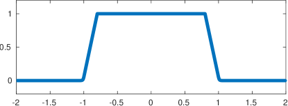
Figure 2: Plot of the unnormalized latent density $q$.

Overlapping Charts.

Since the sets $U_{k}$ of an atlas $(U_{k},\varphi_{k})_{k\in I}$ are an open covering of the manifold, they have to overlap near their boundaries. To this end, we propose the following post-processing heuristic.

By the definition of the loss function $\mathcal{L}$, we have that the $k$-th generator $\mathcal{D}_{k}$ is trained such that $U_{k}$ contains all points $x_{i}$ from the training set where $\tilde{\beta}_{ik}$ is non-zero. The following procedure modifies the $\tilde{\beta}_{ik}$ in such a way that the samples $x$ that are close to the boundary of the $k$-th chart will also be assigned to a second chart.

Since the measure $P_{\Xi}$ is mostly concentrated in $(-1,1)^{d}$, the region close to the boundary of the $k$-th chart can be identified by $D_{k}(\mathcal{T}_{k}(z))$ for all $z$ close to the boundary of $(-1,1)^{d}$. For $c>1$, we define the modified ELBO function

$$\mathrm{ELBO}_{c}(x|\theta_{k}) \coloneqq\mathbb{E}_{\xi\sim\mathcal{N}(0,I_{d})}[\log(p_{\Xi}(c\mathcal{T}_{k}^{-1}(E_{k}(x)+\sigma_{z}\xi)))$$ (14)

$$+\log(|\mathrm{det}(\nabla\mathcal{T}_{k}^{-1}(E_{k}(x)+\sigma_{z}\xi))|)-\tfrac{1}{2\sigma_{x}^{2}}\|D_{k}(E_{k}(x)+\sigma_{z}\xi)-x\|^{2}]$$

which differs from (10) by the additional scaling factor $c$ within the first summand. By construction and by the definiton of $p_{\Xi}$, it holds that $\mathrm{ELBO}_{c}(x,\theta_{k})\approx\mathrm{ELBO}(x|\theta_{k})$ whenever $c\|\mathcal{T}_{k}^{-1}(E_{k}(x))\|_{\infty}<0.8$ and $0<\sigma_{z}\ll 0.1$ is small. Otherwise, we have $\mathrm{ELBO}_{c}(x|\theta_{k})<\mathrm{ELBO}(x|\theta_{k})$ In particular, $\mathrm{ELBO}_{c}(x|\theta_{k})$ is close to $\mathrm{ELBO}(x|\theta_{k})$ if $x$ belongs to the interior of the $k$-th chart and is significantly smaller if it is close to the boundary of the $k$-th chart.

As a variation of $\tilde{\beta}_{ik}$, now we define

$$\hat{\gamma}_{il}^{(l)}=\frac{\alpha_{l}\exp(\mathrm{ELBO}_{c}(x_{i}|\theta_{l}))}{\alpha_{l}\exp(\mathrm{ELBO}_{c}(x_{i}|\theta_{l}))+\sum_{j\in\{1,\dots,K\}\setminus\{l\}}\alpha_{j}\exp(\mathrm{ELBO}(x_{i}|\theta_{j}))}$$

and

$$\hat{\gamma}_{ik}^{(l)}=\frac{\alpha_{k}\exp(\mathrm{ELBO}(x_{i}|\theta_{k}))}{\alpha_{l}\exp(\mathrm{ELBO}_{c}(x_{i}|\theta_{l}))+\sum_{j\in\{1,\dots,K\}\setminus\{l\}}\alpha_{j}\exp(\mathrm{ELBO}(x_{i}|\theta_{j}))}$$

for $k,l\in\{1,\dots,K\}$. Similarly as the $\tilde{\beta}_{ik}$, $\hat{\gamma}_{ik}^{(l)}$ can be viewed as a classification parameter, which assigns each $x_{i}$ either to a chart $k\neq l$ or to the interior part of the $l$-th chart. Consequently, points located near the boundary of the $l$-th chart will also be assigned to another chart. Finally, we combine and normalize the $\hat{\gamma}_{ik}^{(l)}$ by

$$\gamma_{ik}=\frac{\hat{\gamma}_{ik}}{\sum_{k=1}^{K}\hat{\gamma}_{ik}},\quad\text{where}\quad\hat{\gamma}_{ik}=\max_{l=1,\dots,K}\hat{\gamma}_{ik}^{(l)}.$$ (15)

Once, the $\gamma_{ik}$ are computed, we update the mixing weights $\alpha$ by $\alpha_{k}=\sum_{i=1}^{N}\gamma_{ik}$ and minimize the loss function

$$\mathcal{L}_{\text{overlap}}(\Theta)=-\sum_{i=1}^{N}\sum_{k=1}^{K}\gamma_{ik}\mathrm{ELBO}(x_{i}|\theta_{k})$$ (16)

using a certain number of epochs of the Adam optimizer [56].

The whole training procedure for a mixture of VAEs representing the charts of an embedded manifold is summarized in Algorithm 1.

1. Run the Adam optimizer on $\mathcal{L}(\Theta)+\lambda\mathcal{R}(\Theta)$ for $50$ epochs.

2. Run the Adam optimizer on $\mathcal{L}(\Theta)$ for $150$ epochs.

3. Compute the values $\gamma_{ik}$, $i=1,\dots,N$, $k=1,\dots,K$ from (15).

4. Compute the mixing weights $\alpha_{k}=\sum_{i=1}^{N}\gamma_{ik}$.

5. Run the Adam optimizer on $\mathcal{L}_{\text{overlap}}(\Theta)$ from (16) for $50$ epochs.

Algorithm 1 Training procedure for mixtures of VAEs.

3.2 Architectures

In this subsection, we focus on the architecture of the VAEs used in the mixture model representing the manifold $\mathcal{M}$. Since $\mathcal{D}_{k}=D_{k}\circ\mathcal{T}_{k}$ represent the inverse of our charts $\varphi_{k}$, the decoders have to be injective. Moreover, since $\mathcal{E}_{k}=\mathcal{T}_{k}^{-1}\circ E_{k}$ represents the chart itself, the condition $\mathcal{E}_{k}\circ\mathcal{D}_{k}=\mathrm{Id}$ must be verified. Therefore, we choose the encoder $E_{k}$ as a left-inverse of the corresponding decoder $D_{k}$. More precisely, we use the decoders of the form

$$D_{k}=T_{L}\circ A_{L}\circ\cdots\circ T_{1}\circ A_{1},$$ (17)

where the $T_{l}\colon\mathbb{R}^{d_{l}}\to\mathbb{R}^{d_{l}}$ are invertible neural networks and $A_{l}\colon\mathbb{R}^{d_{l-1}}\to\mathbb{R}^{d_{l}}$ are fixed injective linear operators for $l=1,\dots,L$, $d=d_{0}<d_{1}<\cdots<d_{L}=n$. As it is a concatenation of injective mappings, we obtain that $D_{k}$ is injective. Finally, the corresponding encoder is given by

$$E_{k}=A_{1}^{\dagger}\circ T_{1}^{-1}\circ\cdots\circ A_{L}^{\dagger}\circ T_{L}^{-1},\quad A^{\dagger}=(A^{\mathrm{T}}A)^{-1}A^{\mathrm{T}}.$$ (18)

Then, it holds by construction that $\mathcal{E}_{k}\circ\mathcal{D}_{k}=\mathrm{Id}$.

In this paper, we build the invertible neural networks $T_{l}$ and the normalizing flows $\mathcal{T}_{k}$ out of coupling blocks as proposed in [8] based on the real NVP architecture [32]. To this end, we split the input $z\in\mathbb{R}^{d_{l}}$ into two parts $z=(z_{1},z_{2})\in\mathbb{R}^{d_{l}^{1}}\times\mathbb{R}^{d_{l}^{2}}$ with $d_{l}=d_{l}^{1}+d_{l}^{2}$ and define $T_{l}(z)=(x_{1},x_{2})$ with

$$x_{1}=z_{1}\,\mathrm{e}^{s_{2}(z_{2})}+t_{2}(z_{2})\quad\text{and}\quad x_{2}=z_{2}\,\mathrm{e}^{s_{1}(x_{1})}+t_{1}(x_{1}),$$

where $s_{1},t_{1}\colon\mathbb{R}^{d_{l}^{1}}\to\mathbb{R}^{d_{l}^{2}}$ and $s_{2},t_{2}\colon\mathbb{R}^{d_{l}^{2}}\to\mathbb{R}^{d_{l}^{1}}$ are arbitrary subnetworks (depending on $l$). Then, the inverse $T_{l}^{-1}(x_{1},x_{2})$ can analytically be derived as $z=(z_{1},z_{2})$ with

$$z_{2}=\big{(}x_{2}-t_{1}(x_{1})\big{)}\,\mathrm{e}^{-s_{1}(x_{1})}\quad\text{and}\quad z_{1}=\big{(}x_{1}-t_{2}(z_{2})\big{)}\,\mathrm{e}^{-s_{2}(z_{2})}.$$

Remark 2 (Projection onto learned charts).

Consider a decoder $D_{k}$ and an encoder $E_{k}$ as defined above. By construction, the mapping $\pi_{k}=D_{k}\circ E_{k}$ is a (nonlinear) projection onto $\mathrm{range}(D_{k})=\mathrm{range}(\pi_{k})$, in the sense that $\pi_{k}\circ\pi_{k}=\pi_{k}$ and that $\pi_{k|\mathrm{range}(D_{k})}$ is the identity on $\mathrm{range}(D_{k})$. Consequently, the mapping $\pi_{k}$ is a projection on the range of $D_{k}$ which represents the $k$-th chart of $\mathcal{M}$. In particular, there is an open neighborhood $V\coloneqq\pi_{k}^{-1}(U_{k})\subseteq\mathbb{R}^{n}$ such that $\pi_{k|V}$ is a projection onto $U_{k}$.

4 Optimization on Learned Manifolds

As motivated in the introduction, we are interested in optimization problems of the form

$$\min_{x\in\mathbb{R}^{n}}F(x)\quad\text{subject to}\quad x\in\mathcal{M},$$ (19)

where $F\colon\mathbb{R}^{n}\to\mathbb{R}$ is a differentiable function and $\mathcal{M}$ is available only through some data points. In the previous section, we proposed a way to represent the manifold $\mathcal{M}$ by a mixture model $(D_{k},E_{k},\mathcal{T}_{k})$ of VAEs. This section outlines a gradient descent algorithm for the solution of (19) once the manifold is learned.

As outlined in the previous section, the inverse charts $\varphi_{k}^{-1}$ of the manifold $\mathcal{M}$ are modeled by $\mathcal{D}_{k}\coloneqq D_{k}\circ\mathcal{T}_{k}$. The chart $\varphi_{k}$ itself is given by the mapping $\mathcal{E}_{k}\coloneqq\mathcal{T}_{k}^{-1}\circ E_{k}$ restricted to the manifold. For the special case of a VAE with a single generator $\mathcal{D}$, the authors of [4, 23, 33] propose to solve (19) in the latent space. More precisely, starting with a latent initialization $z_{0}\in\mathbb{R}^{d}$ they propose to solve

$$\min_{z\in\mathbb{R}^{d}}F(\mathcal{D}(z))$$

using a gradient descent scheme. However, when using multiple charts, such a gradient descent scheme heavily depends on the current chart. Indeed, the following example shows that the gradient direction can change significantly, if we use a different chart.

Example 3.

Consider the two-dimensional manifold $\mathbb{R}^{2}$ and the two learned charts given by the generators

$$\mathcal{D}_{1}(z_{1},z_{2})=(10z_{1},z_{2}),\quad\text{and}\quad\mathcal{D}_{2}(z_{1},z_{2})=(z_{1},10z_{2}).$$

Moreover let $F\colon\mathbb{R}^{2}\to\mathbb{R}$ be given by $(x,y)\mapsto x+y$. Now, the point $x^{(0)}=(0,0)$ corresponds for both charts to $z^{(0)}=(0,0)$. A gradient descent step with respect to $F\circ\mathcal{D}_{k}$, $k=1,2$, using step size $\tau$ yields the latent values

$$(z_{1}^{(1)},z_{2}^{(1)}) =z^{(0)}-\tau\nabla(F\circ\mathcal{D}_{1})(z^{(0)})=-(10\tau,\tau),$$ (20)

$$(\tilde{z}_{1}^{(1)},\tilde{z}_{2}^{(1)}) =z^{(0)}-\tau\nabla(F\circ\mathcal{D}_{2})(z^{(0)})=-(\tau,10\tau).$$ (21)

Thus, one gradient steps with respect to $F\circ\mathcal{D}_{k}$ yields the values

$$x^{(1)}=\mathcal{D}_{1}(z^{(1)})=-(100\tau,\tau),\quad\tilde{x}^{(1)}=\mathcal{D}_{2}(\tilde{z}^{(1)})=-(\tau,100\tau).$$

Consequently, the gradient descent steps with respect to two different charts can point into completely different directions, independently of the step size $\tau$.

Therefore, we aim to use a gradient formulation which is independent of the parameterization of the manifold. Here, we use the concept of the Riemannian gradient with respect to the Riemannian metric, which is inherited from the Euclidean space in which the manifold $\mathcal{M}$ is embedded. To this end, we first revisit some basic facts about Riemannian gradients on embedded manifolds which can be found, e.g., in [1]. Afterwards, we consider suitable retractions in order to perform a descent step in the direction of the negative Riemannian gradient. Finally, we use these notions in order to derive a gradient descent procedure on a manifold given by mixtures of VAEs.

Riemannian Gradients on Embedded Manifolds.

Let $x\in\mathcal{M}\subseteq\mathbb{R}^{n}$ be a point on the manifold, let $\varphi\colon U\to\mathbb{R}^{d}$ be a chart with $x\in U$ and $\varphi^{-1}\colon\varphi(U)\to U$ be its inverse. Then, the tangent space is given by the set of all directions $\dot{\gamma}(0)$ of differentiable curves $\gamma\colon(-\epsilon,\epsilon)\to\mathcal{M}$ with $\gamma(0)=x$. More precisely, it is given by the linear subspace of $\mathbb{R}^{n}$ defined as

$$T_{x}\mathcal{M}=\{Jy\mathrel{\mathop{\ordinarycolon}}y\in\mathbb{R}^{d}\},\quad\text{ where }J\coloneqq\nabla\varphi^{-1}(\varphi(x))\in\mathbb{R}^{n\times d}.$$ (22)

The tangent space inherits the Riemannian metric from $\mathbb{R}^{n}$, i.e., we equip the tangent space with the inner product

$$\langle u,v\rangle_{x}=u^{\mathrm{T}}v,\quad u,v\in T_{x}\mathcal{M}.$$

A function $f\colon\mathcal{M}\to\mathbb{R}^{m}$ is called differentiable if for any differentiable curve $\gamma\colon(-\epsilon,\epsilon)\to\mathcal{M}$ we have that $f\circ\gamma\colon(-\epsilon,\epsilon)\to\mathbb{R}^{m}$ is differentiable. In this case the differential of $f$ is defined by

$$Df(x)\colon T_{x}\mathcal{M}\to\mathbb{R}^{m},\qquad Df(x)[h]=\frac{\,\mathrm{d}}{\,\mathrm{d}t}f(\gamma_{h}(t))\Big{|}_{t=0},$$

where $\gamma_{h}\colon(-\epsilon,\epsilon)\to\mathcal{M}$ is a curve with $\gamma_{h}(0)=x$ and $\dot{\gamma}_{h}(0)=h$. Finally, the Riemannian gradient of a differentiable function $f\colon\mathcal{M}\to\mathbb{R}$ is given by the unique element $\nabla_{\mathcal{M}}f\in T_{x}\mathcal{M}$ which fulfills

$$Df(x)[h]=\langle\nabla_{\mathcal{M}}f,h\rangle_{x}\quad\text{for all}\quad h\in T_{x}\mathcal{M}.$$

Remark 4.

In the case that $f$ can be extended to a differentiable function on a neighborhood of $\mathcal{M}$, these formulas can be simplified. More precisely, we have that the differential is given by $Df(x)[h]=h^{\mathrm{T}}\nabla f(x)$, where $\nabla f$ is the Euclidean gradient of $f$. In other words, $Df(x)$ is the Fréchet derivative of $f$ at $x$ restricted to $T_{x}\mathcal{M}$. Moreover, the Riemannian gradient coincides with the orthogonal projection of $\nabla f$ on the tangent space, i.e.,

$$\nabla_{\mathcal{M}}f(x)=P_{T_{x}\mathcal{M}}(\nabla f(x)),\quad P_{T_{x}\mathcal{M}}(y)=\operatorname*{arg\,min}_{z\in T_{x}\mathcal{M}}\|y-z\|^{2}.$$

Here the orthogonal projection can be rewritten as $P_{T_{x}\mathcal{M}}=J(J^{\mathrm{T}}J)^{-1}J^{\mathrm{T}}$, $J=\nabla\varphi^{-1}(\varphi(x))$ such that the Riemannian gradient is given by $\nabla_{\mathcal{M}}f(x)=J(J^{\mathrm{T}}J)^{-1}J^{\mathrm{T}}\nabla f(x)$.

Retractions.

Once the Riemannian gradient is computed, we aim to perform a descent step in the direction of $-\nabla_{\mathcal{M}}f(x)$ on $\mathcal{M}$. To this end, we need the concept of retraction. Roughly speaking, a retraction in $x$ maps a tangent vector $\xi$ to the point that is reached by moving from $x$ in the direction $\xi$. Formally, it is defined as follows.

Definition 5.

A differentiable mapping $R_{x}\colon V_{x}\to\mathcal{M}$ for some neighborhood $V_{x}\subseteq T_{x}\mathcal{M}$ of $0$ is called a retraction in $x$, if $R_{x}(0)=x$ and

$$DR_{x}(0)[h]=h\quad\text{for all}\quad h\in T_{0}(V_{x})=T_{x}\mathcal{M},$$

where we identified $T_{0}(V_{x})$ with $T_{x}\mathcal{M}$. Moreover, a differentiable mapping $R=(R_{x})_{x\in\mathcal{M}}\colon V\to\mathcal{M}$ on a subset of the tangent bundle $V=(V_{x})_{x\in\mathcal{M}}\subseteq T\mathcal{M}=(T_{x}\mathcal{M})_{x\in\mathcal{M}}$ is a retraction on $\mathcal{M}$, if for all $x\in\mathcal{M}$ we have that $R_{x}$ is a retraction in $x$.

Now, let $R\colon V\to\mathcal{M}$ be a retraction on $\mathcal{M}$. Then, the Riemannian gradient descent scheme starting at $x_{0}\in\mathcal{M}$ with step size $\tau>0$ is defined by

$$x_{t+1}=R_{x_{t}}(-\tau\nabla_{\mathcal{M}}f(x_{t})).$$

In order to apply this gradient scheme for a learned manifold given by the learned mappings $(\mathcal{D}_{k},\mathcal{E}_{k})_{k=1}^{K}$, we consider two types of retractions. We introduce them and show that they are indeed retractions in the following lemmas. The first one generalizes the idea from [2, Lemma 4, Proposition 5] of moving along the tangent vector in $\mathbb{R}^{n}$ and reprojecting onto the manifold. However, the results from [2] are based on the orthogonal projection, which is hard or even impossible to compute. Thus, we replace it by some more general projection $\pi$. In our applications, $\pi$ will be chosen as in Remark 2, i.e., we set $\pi(x)=\mathcal{D}_{k}(\mathcal{E}_{k}(x)).$

Lemma 6.

Let $x\in\mathcal{M}$, $U_{x}\subseteq\mathbb{R}^{n}$ be a neighborhood of $x$ in $\mathbb{R}^{n}$, $\pi\colon U_{x}\to\mathcal{M}\cap U_{x}$ be a differentiable map such that $\pi\circ\pi=\pi$. Set $V_{x}=\{h\in T_{x}\mathcal{M}\subseteq\mathbb{R}^{n}\mathrel{\mathop{\ordinarycolon}}x+h\in U_{x}\}$. Then

$$R_{x}(h)=\pi(x+h),\qquad h\in V_{x},$$

defines a retraction in $x$.

Proof.

The property $R_{x}(0)=x$ is directly clear from the definition of $R_{x}$. Now let $h\in T_{x}\mathcal{M}\subseteq\mathbb{R}^{n}$ and $\gamma_{h}\colon(-\epsilon,\epsilon)\to\mathcal{M}$ be a differentiable curve with $\gamma_{h}(0)=x$ and $\dot{\gamma}_{h}(0)=h$. As ${\pi}_{|U}$ is the identity on $\mathcal{M}$, we have by the chain rule that

$$h=\dot{\gamma}_{h}(t)=\frac{\,\mathrm{d}}{\,\mathrm{d}t}\pi(\gamma_{h}(t))\Big{|}_{t=0}=\nabla\pi(x)\dot{\gamma}_{h}(0)=\nabla\pi(x)h,$$

where $\nabla\pi(x)$ is the Euclidean Jacobian matrix of $\pi$ at $x$. Similarly,

$$DR_{x}(0)[h]=\frac{\,\mathrm{d}}{\,\mathrm{d}t}R_{x}(th)\Big{|}_{t=0}=\frac{\,\mathrm{d}}{\,\mathrm{d}t}\pi(x+th)\Big{|}_{t=0}=\nabla\pi(x)h=h.\qed$$

The second retraction uses the idea of changing to local coordinates, moving into the gradient direction by using the local coordinates and then going back to the manifold representation. Note that similar constructions are considered in [1, Section 4.1.3]. However, as we did not find an explicit proof for the lemma, we give it below for the sake of completeness.

Lemma 7.

Let $x\in\mathcal{M}$ and denote by $\varphi\colon U\to\mathbb{R}^{d}$ a chart with $x\in U\subseteq\mathcal{M}$. Then,

$$R_{x}(h)=\varphi^{-1}(\varphi(x)+(J^{\mathrm{T}}J)^{-1}J^{\mathrm{T}}h),\quad J=\nabla\varphi^{-1}(\varphi(x))$$

defines a retraction in $x$.

Proof.

The property $R_{x}(0)=x$ is directly clear from the definition of $R_{x}$. Now let $h\in T_{0}(T_{x}\mathcal{M})=T_{x}\mathcal{M}\subseteq\mathbb{R}^{n}$. By (22), we have that there exists some $y\in\mathbb{R}^{d}$ such that $h=Jy$. Then, we have by the chain rule that

$$DR_{x}(0)[h]=\frac{\,\mathrm{d}}{\,\mathrm{d}t}R_{x}(th)\Big{|}_{t=0}=(\nabla\varphi^{-1}(\varphi(x)))(J^{\mathrm{T}}J)^{-1}J^{\mathrm{T}}h=J(J^{\mathrm{T}}J)^{-1}J^{\mathrm{T}}Jy=Jy=h.$$

∎

Gradient Descent on Learned Manifolds.

By Lemma 6 and 7, we obtain that the mappings

$$R_{k,x}(h)=\mathcal{D}_{k}(\mathcal{E}_{k}(x+h))\quad\text{and}\quad\tilde{R}_{k,x}(h)=\mathcal{D}_{k}(\mathcal{E}_{k}(x)+(J^{\mathrm{T}}J)^{-1}J^{\mathrm{T}}h)$$ (23)

with $J=\nabla\mathcal{D}_{k}(\mathcal{E}_{k}(x))$ are retractions in all $x\in U_{k}$. If we define $R$ such that $R_{x}$ is given by $R_{k}$ for some $k$ such that $x\in U_{k}$, then the differentiability of $R=(R_{x})_{x\in\mathcal{M}}$ in $x$ might be violated. Moreover, the charts learned by a mixture of VAEs only overlap approximately and not exactly. Therefore, these retractions cannot be extended to a retraction on the whole manifold $\mathcal{M}$ in general. As a remedy, we propose the following gradient descent step on a learned manifold.

Starting from a point $x_{n}$, we first compute for $k=1,\dots,K$ the probability, that $x_{n}$ belongs to the $k$-th chart. By (11), this probability can be approximated by

$$\beta_{k}\coloneqq\tfrac{\alpha_{k}\exp(\mathrm{ELBO}(x_{n}|\theta_{k}))}{\sum_{j=1}^{K}\alpha_{j}\exp(\mathrm{ELBO}(x_{n}|\theta_{j}))}.$$ (24)

Afterwards, we project $x_{n}$ onto the $k$-th chart by applying $\tilde{x}_{n,k}=\mathcal{D}_{k}(\mathcal{E}_{k}(x_{n}))$ (see Remark 2) and compute the Riemannian gradient $g_{n,k}=\nabla_{\mathcal{M}}F(\tilde{x}_{n_{k}})$. Then, we apply the retraction $R_{k,\tilde{x}_{n,k}}$ (or $\tilde{R}_{k,\tilde{x}_{n,k}}$) to perform a gradient descent step $x_{n+1,k}=R_{k,\tilde{x}_{n,k}}(-\tau_{n}g_{n,k})$. Finally, we average the results by $x_{n+1}=\sum_{k=1}^{K}\beta_{k}x_{n+1,k}$.

The whole gradient descent step is summarized in Algorithm 2. Finally, we compute the sequence $(x_{n})_{n}$ by applying Algorihtm 2 iteratively.

Inputs: Function $F\colon\mathcal{M}\to\mathbb{R}$, point $x_{n}$, step size $\tau_{n}>0$.

for $k=1,\dots,K$ do

     - Approximate the probability that $x_{n}$ belongs to chart $k$ by computing the $\beta_{k}$

     - from (24).

     - Project to the $k$-th chart by $\tilde{x}_{n,k}=\mathcal{D}_{k}(\mathcal{E}_{k}(x_{n}))$.

     - Compute the Riemannian gradient $g_{n,k}=\nabla_{\mathcal{M}}F(\tilde{x}_{n,k})$, e.g., by Remark 4.

     - Perform a gradient descent with the retraction $R_{k,\tilde{x}_{n,k}}$, i.e., define

     - $x_{n+1,k}=R_{k,\tilde{x}_{n,k}}(-\tau_{n}g_{n,k}).$

end for

- Average results by computing $x_{n+1}=\sum_{k=1}^{K}\beta_{k}x_{n+1,k}.$

Algorithm 2 One gradient descent step on a learned manifold.

For some applications the evaluation of the derivative of $F$ is computationally costly. Therefore, we aim to take as large step sizes $\tau_{n}$ as possible in Algorithm 2. On the other hand, large step sizes can lead to numerical instabilities and divergence. To this end, we use an adaptive step size selection as outlined in Algorithm 3.

Input: Function $F$, initial point $x_{0}$, initial step size $\tau_{0}$.

for n=0,1,… do

     Compute $x_{n+1}$ by Algorithm 2 with step size $\tau_{n}$.

     while $F(x_{n+1})>F(x_{n})$ do

         Update step size by $\tau_{n}\leftarrow\frac{\tau_{n}}{2}$.

         Update $x_{n+1}$ by Algorithm 2 with the new step size $\tau_{n}$.

     end while

     Set step size for the next step $\tau_{n+1}=\frac{3\tau_{n}}{2}$.

end for

Algorithm 3 Adaptive step size scheme for gradient descent on learned manifolds

5 Numerical Examples

Two circles

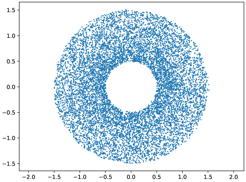
Ring

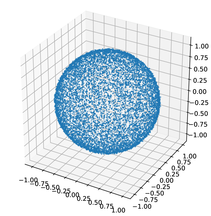
Sphere

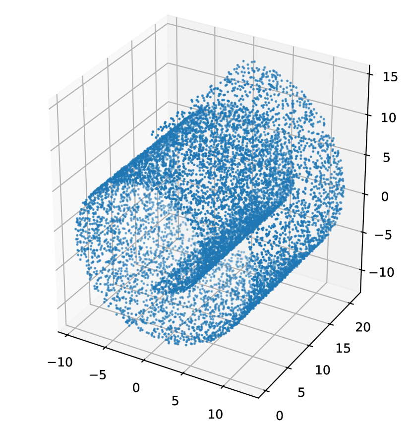
Swiss roll

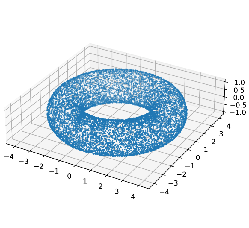
Torus

Figure 3: Datasets used for the different manifolds.

Next, we test the numerical performance of the proposed method. In this section, we start with some one- and two-dimensional manifolds embedded in the two- or three-dimensional Euclidean space. We use the architecture from Section 3.2 with $L=1$. That is, for all the manifolds, the decoder is given by $\mathcal{T}\circ A$ where $A\colon\mathbb{R}^{d}\to\mathbb{R}^{n}$ is given by $x\mapsto(x,0)$ if $d=n-1$ and by $A=\mathrm{Id}$ if $d=n$ and $\mathcal{T}$ is an invertible neural network with $5$ invertible coupling blocks where the subnetworks have two hidden layers and $64$ neurons in each layer. The normalizing flow modelling the latent space consists of $3$ invertible coupling blocks with the same architecture. We train the mixture of VAEs for $200$ epochs with the Adam optimizer. Afterwards we apply the overlapping procedure for $50$ epochs, as in Algorithm 1.

We consider the manifolds “two circles”, “ring”, “sphere”, “swiss roll” and “torus”. The (noisy) training data are visualized in Figure 3. The number of charts $K$ is given in the following table.

	Two circles	Ring	Sphere	Swiss roll	Torus
Number of charts	$4$	$2$	$2$	$4$	$6$

We visualize the learned charts in Figure 4. Moreover, additional samples generated by the learned mixture of VAEs are shown in Figure 5. We observe that our model covers all considered manifolds and provides a reasonable approximation of different charts. Finally, we apply the gradient descent method from Algorithm 2 to the following functions:

• $F(x)=x_{2}$ on the manifold “two circles” with initial points $\frac{x_{0}}{\|x_{0}\|}\pm(1.5,0)$ for $x_{0}=(\pm 0.2,1)$;

• $F(x)=\|x-(-1,0)\|^{2}$ on the manifold “ring” with initial points $(1,\pm 0.4)$;

• $F(x)=\|x-(0,0,-2)\|^{2}$ on the manifold “sphere” with inital points $x_{0}/\|x_{0}\|$ for $x_{0}\in\{(0.3\cos(\tfrac{\pi k}{5}),0.3\sin(\tfrac{\pi k}{5}),1)\mathrel{\mathop{\ordinarycolon}}k=0,\dots,9)\}$;

• $F(x)=\|x-(-5,0,0)\|^{2}$ on the manifold “torus”, where the inital points are drawn randomly from the training set.

We use the retraction from Lemma 6 with a step size of $0.01$. The resulting trajectories are visualized in Figure 6. We observe that all the trajectories behave as expected and approach the closest minimum of the objective function, even if this is not in the same chart of the initial point.

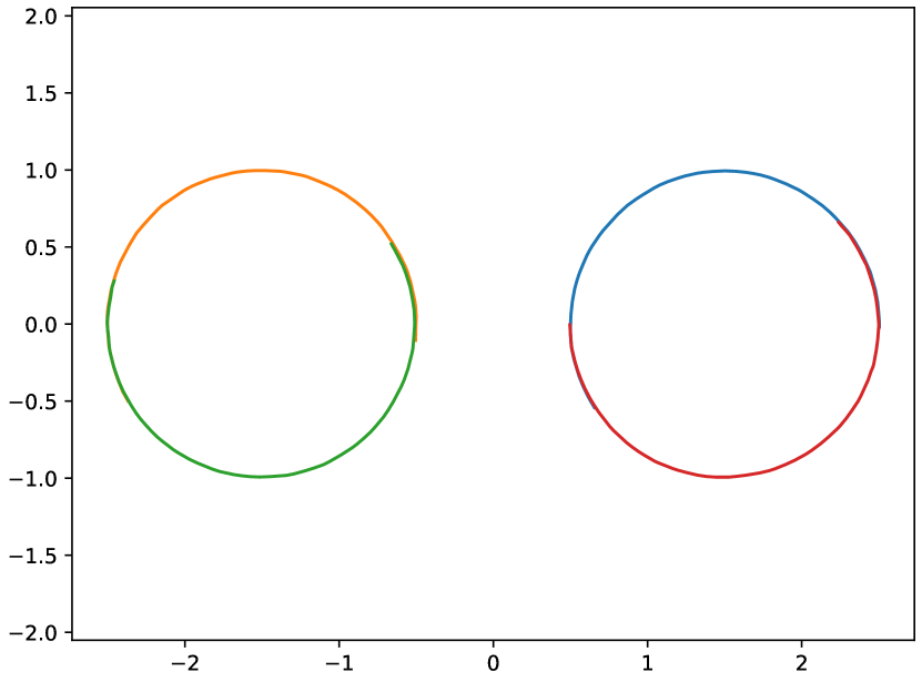
Two circles

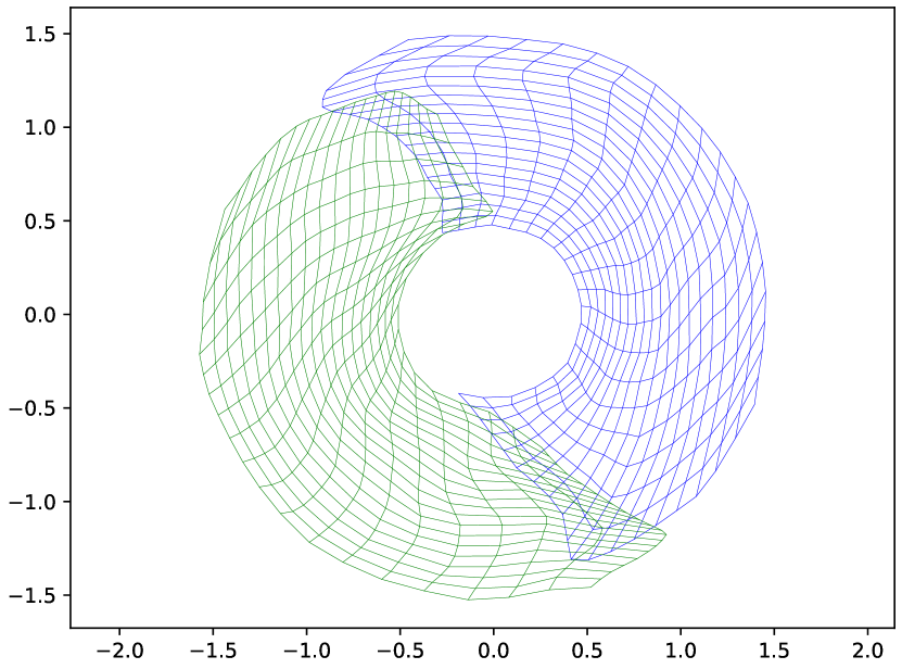
Ring

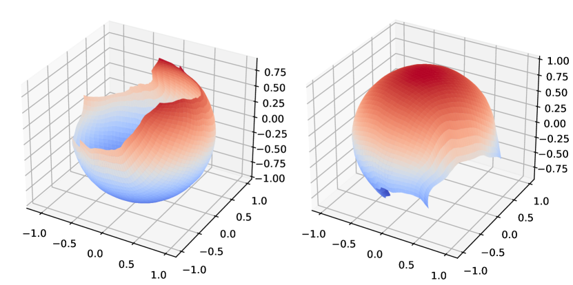
Sphere

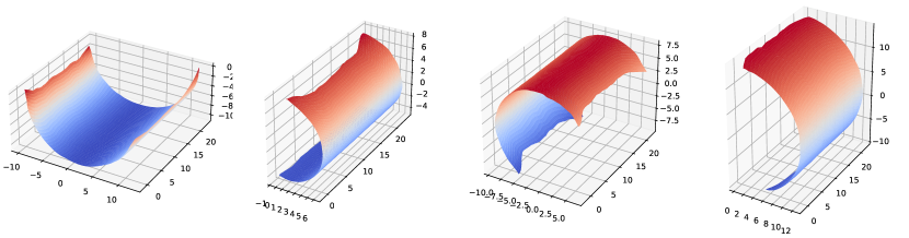
Swiss roll

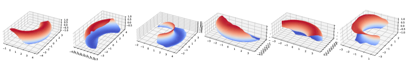
Torus

Figure 4: Learned charts for the different manifolds. For the manifolds “two circles” and “ring”, each color represents one chart. For the manifolds “sphere”, “swiss roll” and “torus” we plot each chart in a separate figure.

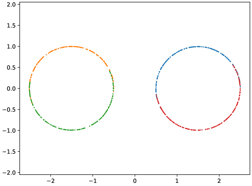
Two circles

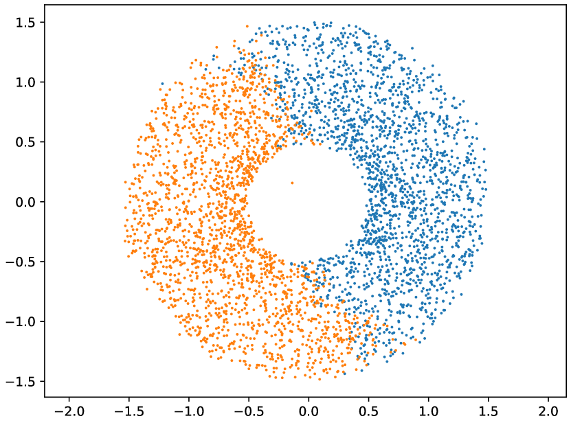
Ring

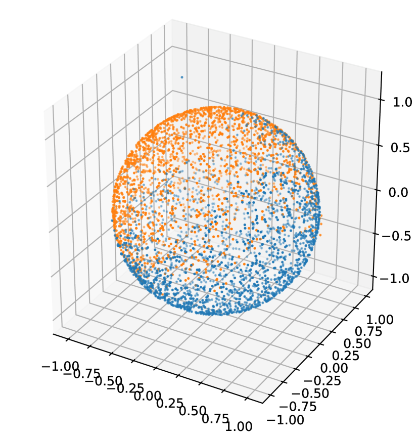
Sphere

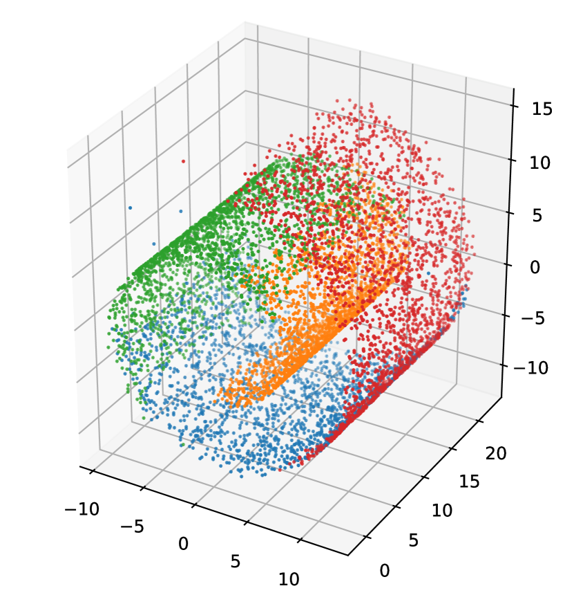
Swiss roll

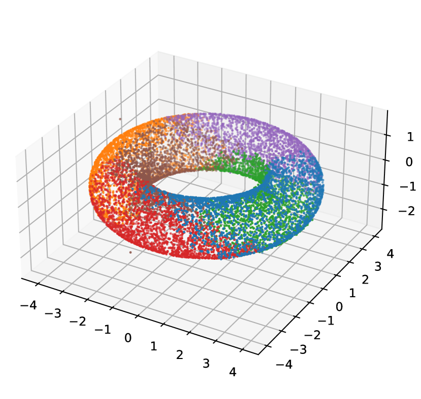
Torus

Figure 5: Generated samples by the learned mixture of VAEs. The color of a point indicates from which generator the point was sampled.

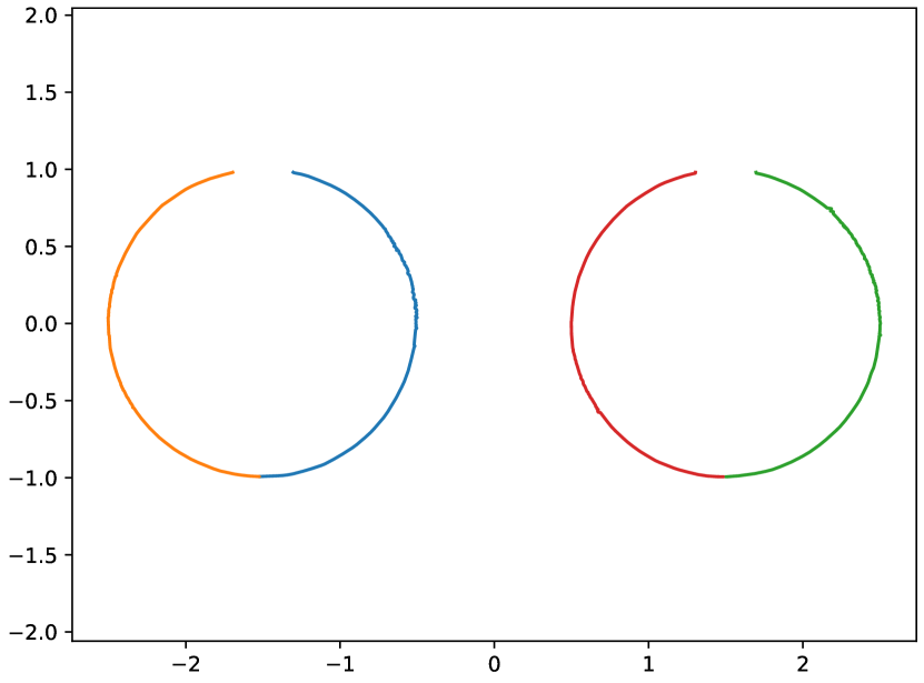
Two circles

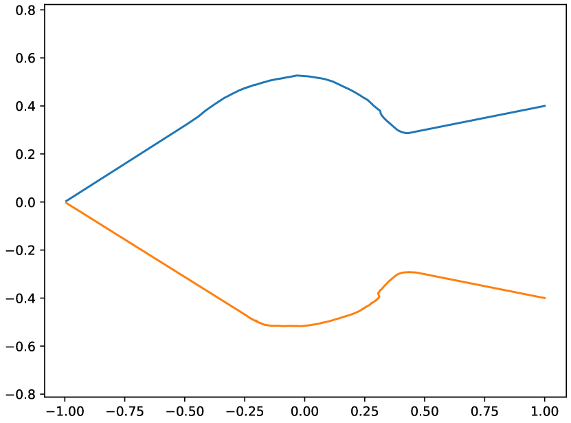
Ring

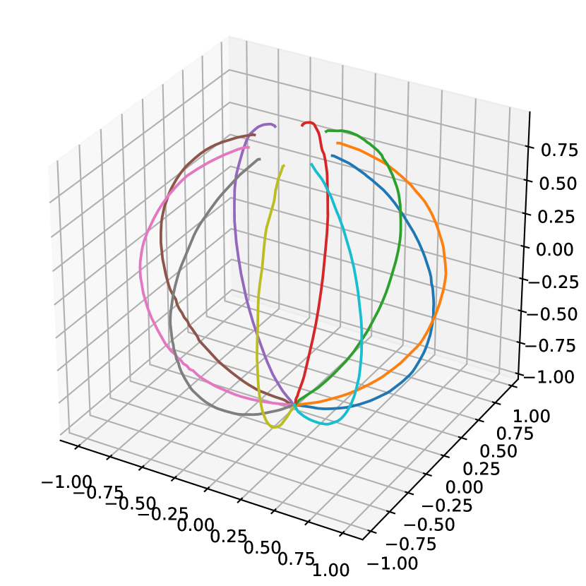
Sphere

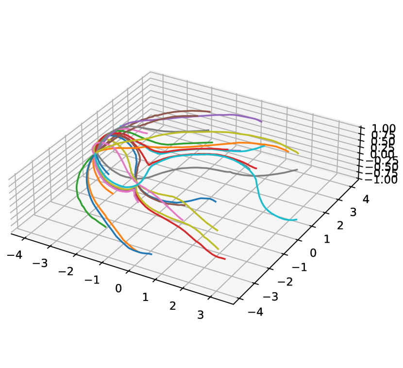
Torus

Figure 6: Trajectories of the gradient descent on the learned manifolds.

Remark 8 (Dimension of the Manifold).

For all our numerical experiments, we assume that the dimension $d$ of the data manifold is known. This assumption might be violated for practical applications. However, there exist several methods in the literature to estimate the dimension of a manifold from data, see e.g., [14, 22, 35, 64]. Combining these methods with our mixture of VAEs is not within the scope of this paper and is left for future research.

6 Mixture of VAEs for Inverse Problems

In this section we describe how to use mixture of VAEs to solve inverse problems. We consider an inverse problem of the form

$$y=\mathcal{G}(x)+\eta,$$ (25)

where $\mathcal{G}$ is a possibly nonlinear map between $\mathbb{R}^{n}$ and $\mathbb{R}^{m}$, modeling a measurement (forward) operator, $x\in\mathbb{R}^{n}$ is a quantity to be recovered, $y\in\mathbb{R}^{m}$ is the noisy data and $\eta$ represents some noise. In particular, we analyze a linear and a nonlinear inverse problem: a deblurring problem and a parameter identification problem for an elliptic PDE arising in electrical impedance tomography (EIT), respectively.

In many inverse problems, the unknown $x$ can be modeled as an element of a low-dimensional manifold $\mathcal{M}$ in $\mathbb{R}^{n}$ [4, 10, 20, 53, 73, 82, 70, 3], and this manifold can be represented by the mixture of VAEs as explained in Section 3. Thus, the solution of (25) can be found by optimizing the function

$$F(x)=\frac{1}{2}\|\mathcal{G}(x)-y\|^{2}_{\mathbb{R}^{m}}\quad\text{subject to }x\in\mathcal{M},$$ (26)

by using the iterative scheme proposed in Section 4.

We would like to emphasize that the main goal of our experiments is not to obtain state-of-the-art results. Instead, we want to highlight the advantages of using multiple generators via a mixture of VAEs. All our experiments are designed in such a way that the manifold property of the data is directly clear. The application to real-world data and the combination with other methods in order to achieve competitive results are not within the scope of this paper and are left to future research.

Architecture and Training.

Throughout these experiments we consider images of size $128\times 128$ and use the architecture from Section 3.2 with $L=3$. Starting with the latent dimension $d$, the mapping $A_{1}\colon\mathbb{R}^{d}\to\mathbb{R}^{32^{2}}$ fills up the input vector $x$ with zeros up to the size $32^{2}$, i.e., we set $A_{1}(x)=(x,0)$. The invertible neural network $T_{1}\colon\mathbb{R}^{32^{2}}\to\mathbb{R}^{32^{2}}$ consists of $3$ invertible blocks, where the subnetworks $s_{i}$ and $t_{i}$, $i=1,2$ are dense feed-forward networks with two hidden layers and $64$ neurons. Afterwards, we reorder the dimensions to obtain an image of size $32\times 32$. The mappings $A_{2}\colon\mathbb{R}^{32\times 32}\to\mathbb{R}^{32\times 32\times 4}$ and $A_{3}\colon\mathbb{R}^{64\times 64}\to\mathbb{R}^{64\times 64\times 4}$ copy each channel $4$ times. Then, the generalized inverses $A_{2}^{\dagger}\colon\mathbb{R}^{32\times 32\times 4}\to\mathbb{R}^{32\times 32}$ and $A_{3}^{\dagger}\colon\mathbb{R}^{64\times 64\times 4}\to\mathbb{R}^{64\times 64}$ from (18) are given by taking the mean of the four channels of the input. The invertible neural networks $T_{2}\colon\mathbb{R}^{32\times 32\times 4}\to\mathbb{R}^{64\times 64}$ and $T_{3}\colon\mathbb{R}^{64\times 64\times 4}\to\mathbb{R}^{128\times 128}$ consist of $3$ invertible blocks, where the subnetworks $s_{i}$ and $t_{i}$, $i=1,2$ are convolutional neural networks with one hidden layer and $64$ channels. After these three coupling blocks we use an invertible upsampling [34] to obtain the correct output dimension. For the normalizing flow in the latent space, we use an invertible neural network with three blocks, where the subnetworks $s_{i}$ and $t_{i}$, $i=1,2$ are dense feed-forward networks with two hidden layers and $64$ neurons.

We train all the models for 200 epochs with the Adam optimizer. Afterwards we apply the overlapping procedure for $50$ epochs. See Algorithm 1 for the details of the training algorithm.

6.1 Deblurring

(a) Samples from the considered dataset for the deblurring example.

(b) Learned chart with one generator. The figure shows the images $D(x)$ for $20$ values of $x$ equispaced in $[-1,1]$.

(c) Learned charts with two generators. The figure shows the images $D_{k}(x)$ for $20$ values of $x$ equispaced in $[-1,1]$ for $k=1$ (top) and $k=2$ (bottom).

(d) Reconstructions for the deblurring example. From top to bottom: ground truth image, observation, reconstruction with one generator and reconstruction with two generators.

Figure 7: Dataset, learned charts and reconstructions for the deblurring example.

(a) Ground truth (left) and observation (right).

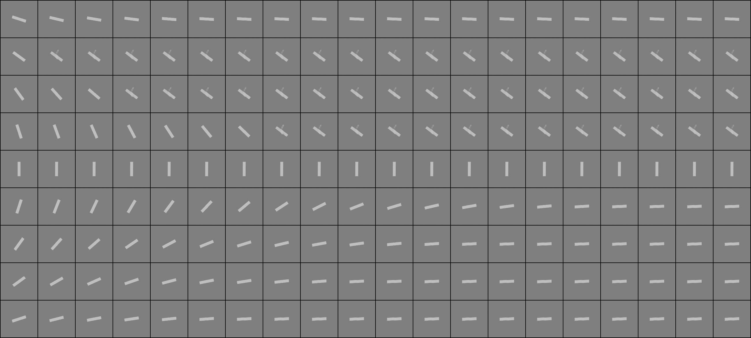
(b) Visualization of the trajectories $(x_{n})_{n}$ for different initializations $x_{0}$ with one generator. Left column: initialization, right column: reconstruction $x_{250}$, columns in between: images $x_{n}$ for $n$ approximately equispaced between $0$ and $250$.

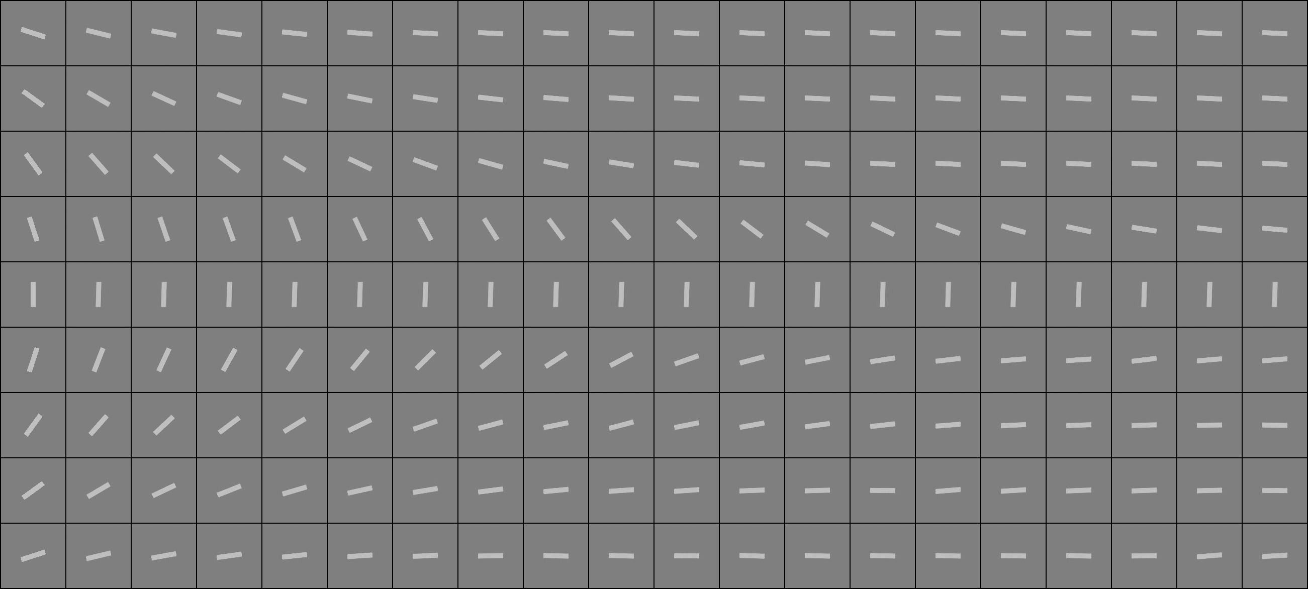
(c) Visualization of the trajectories $(x_{n})_{n}$ for different initializations $x_{0}$ with two generators. Left column: initialization, right column: reconstruction $x_{250}$, columns in between: images $x_{n}$ for $n$ approximately equispaced between $0$ and $250$.

Figure 8: Gradient descent for the deblurring example.

First, we consider the inverse problem of noisy image deblurring. Here, the forward operator $\mathcal{G}$ in (25) is linear and given by the convolution with a $30\times 30$ Gaussian blur kernel with standard deviation $15$. In order to obtain outputs $y$ of the same size as the input $x$, we use constant padding with intensity $1/2$ within the convolution. Moreover, the image is corrupted by white Gaussian noise $\eta$ with standard deviation $0.1$. Given an observation $y$ generated by this degradation process, we aim to reconstruct the unknown ground truth image $x$.

Dataset and Manifold Approximation.

Here, we consider the dataset of $128\times 128$ images showing a bright bar with a gray background which is centered and rotated. The intensity of fore- and background as well as the size of the bar are fixed. Some example images from the dataset are given in Figure 7(a). The dataset forms a one-dimensional manifold parameterized by the rotation of the bar. Therefore, it is homeomorphic to $S^{1}$ and does not admit a global parameterization since it contains a hole.

We approximate the data manifold by a mixture model of two VAEs and compare the result with the approximation with a single VAE, where the latent dimension is set to $d=1$. The learned charts are visualized in Figure 7(b) and 7(c). We observe that the chart learned with a single VAE does not cover all possible rotations of the bar, while the mixture of two VAEs can generate any rotation. Moreover, we can see that the two charts of the mixture of VAEs overlap.

Reconstruction.

In order to reconstruct the ground truth image, we use our gradient descent scheme for the function (26) as outlined in Algorithm 2 for 500 iterations. Since the function $F$ is defined on the whole $\mathbb{R}^{128\times 128}$, we compute the Riemannian gradient $\nabla_{\mathcal{M}}F(x)$ accordingly to Remark 4. More precisely, for $x\in U_{k}$, we have $\nabla_{\mathcal{M}}F(x)=J(J^{\mathrm{T}}J)^{-1}J^{\mathrm{T}}\nabla F(x)$, where $\nabla F(x)$ is the Euclidean gradient of $F$ and $J=\nabla\mathcal{D}_{k}(\mathcal{E}_{k}(x))$ is the Jacobian of the $k$-th decoder evaluated at $\mathcal{E}_{k}(x)$. Here, the Euclidean gradient $\nabla F(x)$ and the Jacobian matrix $J$ are computed by algorithmic differentiation. Moreover, we use the retractions $\tilde{R}_{k,x}$ from (23). As initialization $x_{0}$ of our gradient descent scheme, we use a random sample from the mixture of VAEs. The results are visualized in Figure 7(d). We observe that the reconstructions with two generators always recover the ground truth images very well. On the other hand, the reconstructions with one generator often are unrealistic and do not match with the ground truth. These unrealistic images appear at exactly those points where the chart of the VAE with one generator does not cover the data manifold.

In order to better understand why the reconstructions with one generator often fail, we consider the trajectories $(x_{n})_{n}$ generated by Algorithm 2 more in detail. We consider a fixed ground truth image showing a horizontal bar and a corresponding observation as given in Figure 8(a). Then, we run Algorithm 2 for different initializations. The results are given in Figure 8(b) for one generator and in Figure 8(c) for two generators. The left column shows the initialization $x_{0}$, and in the right column, there are the values $x_{250}$ after 250 gradient descent steps. The columns in between show the values $x_{n}$ for (approximately) equispaced $n$ between $0$ and $250$. With two generators, the trajectory $(x_{n})_{n}$ are a smooth transition from the initialization to the ground truth. Only when the initialization is a vertical bar (middle row), the images $x_{n}$ remain similar to the initialization $x_{0}$ for all $n$, since this is a critical point of the $F|_{\mathcal{M}}$ and hence the Riemannian gradient is zero. With one generator, we observe that some of the trajectories get stuck. This emphasizes the need for multiple generators.

6.2 Electrical Impedance Tomography

(a) Samples from the considered dataset for the EIT example.

(b) Samples from the VAE with one generator.

(c) Samples from the mixture of two VAEs. Top: first chart, bottom: second chart.

(d) Reconstructions. From top to bottom: ground truth image, reconstruction with one generator, reconstruction with two generators.

Figure 9: Dataset, synthesized samples and reconstructions for the EIT example.

Finally, we consider the highly non-linear and ill-posed inverse problem of electrical impedance tomography (EIT) [27], which is also known in the mathematical literature as the Calderón problem [12, 37, 72]. EIT is a non-invasive, radiation-free method to measure the conductivity of a tissue through electrodes placed on the surface of the body. More precisely, electrical currents patterns are imposed on some of these electrodes and the resulting voltage differences are measured on the remaining ones. Although harmless, the use of this modality in practice is very limited because the standard reconstruction methods provide images with very low spatial resolution. This is an immediate consequence of the severe ill-posedness of the inverse problem [5, 69].

Classical methods for solving this inverse problem include variational-type methods [28], the Lagrangian method [26], the factorization method [21, 60], the D-bar method [84], the enclosure method [54], and the monotonicity method [87]. Similarly as many other inverse problems, deep learning methods have had a big impact on EIT. For example, the authors of [36] propose an end-to-end neural network that learns the forward map $\mathcal{G}$ and its inverse. Moreover, deep learning approaches can be combined with classical methods, e.g, by post processing methods [46, 45] or by variational learning algorithms [82].

Dataset and Manifold Approximation.

We consider the manifold consisting of $128\times 128$ images showing two bright non-overlapping balls with a gray background, representing conductivities with special inclusions. The radius and the position of the balls vary, while the fore- and background intensities are fixed. Some exemplary samples of the dataset are given in Figure 9(a). The images from the dataset have six degrees of freedom, namely the positions and the radii of both balls in $\mathbb{R}^{2}$. Therefore, these images form a six-dimensional manifold. Since the balls are not allowed to overlap, the manifold has a nontrivial topology and does not admit a global parameterization.

A slightly more general version of this manifold was considered in [3], where Lipschitz stability is proven for a related inverse boundary value problem restricted to the manifold. Other types of inclusions (with unknown locations), notably polygonal and polyhedral inclusions, have been considered in the literature [18, 17, 11]. The case of small inclusions is discussed in [7].

We approximate the data manifold by a mixture of two VAEs and compare the results with the approximation with a single VAE. The latent dimension is set to the manifold dimension, i.e., $d=6$. Some samples of the learned charts are given in Figure 9(b) and 9(c). As in the previous example, both models produce mostly realistic samples.

The Forward Operator and its Derivative.

From a mathematical viewpoint, EIT considers the following PDE with Neumann boundary conditions

$$\left\{\begin{array}[]{rl}-\nabla\cdot(\gamma\hskip 2.84544pt\nabla u_{g})=0&\text{in }\Omega,\\ \gamma\hskip 2.84544pt\partial_{\nu}u_{g}=g&\text{on }\partial\Omega,\end{array}\right.$$ (27)

where $\Omega\subseteq\mathbb{R}^{2}$ is a bounded domain, $\gamma\in L^{\infty}(\Omega)$ is such that $\gamma(x)\geq\lambda>0$ and $u_{g}\in H^{1}(\Omega)$ is the unique weak solution with zero boundary mean of (27) with Neumann boundary data $g\in H^{-\frac{1}{2}}_{\diamond}(\partial\Omega)$, with $H^{s}_{\diamond}(\partial\Omega)=\{f\in H^{s}(\partial\Omega)\mathrel{\mathop{\ordinarycolon}}\int_{\partial\Omega}fds=0\}$. From the physical point of view, $g$ represents the electric current applied on $\partial\Omega$ (through electrodes placed on the boundary of the body), $u_{g}$ is the electric potential and $\gamma$ is the conductivity of the body in the whole domain $\Omega$. The inverse problem consists in the reconstruction of $\gamma$ from the knowledge of all pairs of boundary measurements $(g,u_{g}|_{\partial\Omega})$, namely, of all injected currents together with the corresponding electric voltages generated at the boundary. In a compact form, the measurements may be modelled by the Neumann-to-Dirichlet map

$$\mathcal{G}(\gamma)\colon H^{-\frac{1}{2}}_{\diamond}(\partial\Omega) \to H^{\frac{1}{2}}_{\diamond}(\partial\Omega)$$

$$g \mapsto u_{g}\big{|}_{\partial\Omega}.$$

Since the PDE (27) is linear, the map $\mathcal{G}(\gamma)$ is linear. However, the forward map $\gamma\mapsto\mathcal{G}(\gamma)$ is nonlinear in $\gamma$, and so is the corresponding inverse problem. The map $\mathcal{G}$ is continuously differentiable, and its Fréchet derivative (see [47]) is given by $[\nabla\mathcal{G}(\gamma)](\sigma)(g)=w_{g}\big{|}_{\partial\Omega}$, where $w_{g}\in H^{1}(\Omega)$ is the unique weak solution with zero boundary mean of

$$\left\{\begin{array}[]{rl}-\nabla\cdot(\gamma\hskip 2.84544pt\nabla w_{g})=\nabla\cdot(\sigma\hskip 2.84544pt\nabla u_{g})&\text{in }\Omega,\\ -\gamma\hskip 2.84544pt\partial_{\nu}w_{g}=\sigma\hskip 2.84544pt\partial_{\nu}u_{g}&\text{on }\partial\Omega,\end{array}\right.$$

where $u_{g}\in H^{1}(\Omega)$ is the unique weak solution with zero boundary mean that solves (27). We included the expression of this derivative in the continuous setting for completeness, but, as a matter of fact, we will need only its semi-discrete counterpart given below.

Discretization and Objective Function.

In our implementations, we discretize the linear mappings $G(\gamma)$ by restricting them to a finite dimensional subspace spanned by a-priori fixed boundary functions $g_{1},\dots,g_{N}\in H^{-\frac{1}{2}}_{\diamond}(\partial\Omega)$. Then, following [19, eqt. (2.2)], we reconstruct the conductivity by minimizing the semi-discrete functional

$$F(\gamma)=\frac{1}{2}\sum_{n=1}^{N}\int_{\partial\Omega}|u_{g_{n}}(s)-(u_{\text{true}})_{g_{n}}(s)|^{2}ds,$$ (28)

where $(u_{\text{true}})_{g_{n}}$ is the observed data. In our discrete setting, we represent the conductivitiy $\gamma$ by a piecewise constant function $\gamma=\sum_{m=1}^{M}\gamma_{m}\mathbbm{1}_{T_{m}}$ on a triangulation $(T_{m})_{m=1,\dots,M}$. Then, following [19, eqt. (2.20)], the derivative of (28) with respect to $\gamma$ is given by

$$\frac{dF}{d\gamma_{m}}(\gamma)=\sum_{n=1}^{N}\int_{T_{m}}\nabla u_{g_{n}}(x)\cdot\nabla z_{g_{n}}(x)dx,$$ (29)

where $z_{g_{n}}$ solves

$$\left\{\begin{array}[]{rl}-\nabla\cdot(\gamma\hskip 2.84544pt\nabla z_{g_{n}})=0\phantom{(u_{\text{true}})_{g_{n}}-u_{g_{n}}}&\text{in }\Omega,\\ \gamma\hskip 2.84544pt\partial_{\nu}z_{g_{n}}=(u_{\text{true}})_{g_{n}}-u_{g_{n}}\phantom{0}&\text{on }\partial\Omega,\end{array}\right.$$ (30)

with the normalization $\int_{\partial\Omega}z_{g_{n}}(s)ds=\int_{\partial\Omega}(u_{\text{true}})_{g_{n}}(s)ds$.

Implementation Details.

In our experiments the domain $\Omega$ is given by the unit square $[0,1]^{2}$. For solving the PDEs (27) and (30), we use a finite element solver from the DOLFIN library [66]. We employ meshes that are coarser in the middle of $\Omega$ and finer close to the boundary. To simulate the approximation error of the meshes, and to avoid inverse crimes, we use a fine mesh to generate the observation and a coarser one for the reconstructions. We use $N=15$ boundary functions, which are chosen as follows. We divide each of the four edges of the unit square $[0,1]^{2}$ into 4 segments and denote by $b_{1},\dots,b_{16}$ the functions that are equal to $1$ on one of these segments and $0$ otherwise. Then, we define the boundary functions as $g_{n}=\sum_{i=1}^{16}a_{n,i}b_{i}$, where the matrix $A=(a_{n,i})_{n=1,\dots,15,i=1,\dots,16}$ is the $16\times 16$ Haar matrix without the first row. More precisely, the rows of $A$ are given by the rows of the matrices $2^{-k/2}(\mathrm{Id}_{2^{4-k}}\otimes(1,-1)\otimes e_{2^{k-1}}^{\mathrm{T}})$ for $k=1,\dots,4$, where $\otimes$ is the Kronecker product and $e_{j}\in\mathbb{R}^{j}$ is the vector where all entries are $1$.

Results.

We reconstruct the ground truth images from the observations by minimizing the functional $F$ from (28) subject to $\gamma\in\mathcal{M}$. To this end, we apply the gradient descent scheme from Algorithm 2 for 100 steps. Since the evaluation of the forward operator and its derivative include the numerical solution of a PDE, it is computationally very costly. Hence, we aim to use as few iterations of Algorithm 2 as possible. To this end, we apply the adaptive step size scheme from Algorithm 3. As retractions we use $\tilde{R}_{k,x}$ from (23). The initialization $\gamma_{0}$ of the gradient descent scheme is given by a random sample from the mixture of VAEs.

Since $F$ is defined on the whole $\mathbb{R}_{+}^{128\times 128}$, we use again Remark 4 for the evaluation of the Riemannian gradient. More precisely, for $\gamma\in U_{k}$, we have that $\nabla_{\mathcal{M}}F(\gamma)=J(J^{\mathrm{T}}J)^{-1}J^{\mathrm{T}}\nabla F(\gamma)$, where $\nabla F(\gamma)$ is the Euclidean gradient of $F$ and $J=\nabla\mathcal{D}_{k}(\mathcal{E}_{k}(\gamma))$. Here, we compute $\nabla F(\gamma)$ by (29) and $J$ by algorithmic differentiation.

The reconstructions for 20 different ground truths are visualized in Figure 9(d). We observe that both models capture the ground truth structure in most cases, but also fail sometimes. Nevertheless, the reconstructions with the mixture of two VAEs recover the correct structure more often and more accurately than the single VAE. To quantify the difference more in detail, we rerun the experiment with $200$ different ground truth images and average the resulting PSNR over $200$ reconstructions within the following table.

	One generator	Two generators
PSNR	$23.64\pm 3.91$	$24.76\pm 3.79$

Consequently, the reconstructions with two generators are significantly better than those with one generator.

7 Conclusions

In this paper we introduced mixture models of VAEs for learning manifolds of arbitrary topology. The corresponding decoders and encoders of the VAEs provide analytic access to the resulting charts and are learned by a loss function that approximates the negative log-likelihood function. For minimizing functions $F$ defined on the learned manifold we proposed a Riemannian gradient descent scheme. In the case of inverse problems, $F$ is chosen as a data-fidelity term. Finally, we demonstrated the advantages of using several generators on numerical examples.

This work can be extended in several directions. First, gradient descent methods converge only locally and are not necessarily fast. Therefore, it would be interesting to extend the minimization of the functional $F$ in Section 19 to higher-order methods or incorporate momentum parameters. Moreover, a careful choice of the initialization could improve the convergence behavior. Further, our reconstruction method could be extended to Bayesian inverse problems. Since the mixture model of VAEs provides us with a probability distribution and an (approximate) density, stochastic sampling methods like the Langevin dynamics could be used for quantifying uncertainties within our reconstructions. Indeed, Langevin dynamics on Riemannian manifolds are still an active area of research. Finally, recent papers show that diffusion models provide an implicit representation of the data manifold [14, 80]. It would be interesting to investigate optimization models on such manifolds in order to apply them to inverse problems.

References

- [1] P.-A. Absil, R. Mahony, and R. Sepulchre. Optimization algorithms on matrix manifolds. In Optimization Algorithms on Matrix Manifolds. Princeton University Press, 2009.
- [2] P.-A. Absil and J. Malick. Projection-like retractions on matrix manifolds. SIAM Journal on Optimization, 22(1):135–158, 2012.
- [3] G. S. Alberti, A. Arroyo, and M. Santacesaria. Inverse problems on low-dimensional manifolds. Nonlinearity, 36(1):734–808, 2023.
- [4] G. S. Alberti, M. Santacesaria, and S. Sciutto. Continuous generative neural networks. arXiv preprint arXiv:2205.14627, 2022.
- [5] G. Alessandrini. Stable determination of conductivity by boundary measurements. Applicable Analysis, 27(1-3):153–172, 1988.
- [6] F. Altekrüger, A. Denker, P. Hagemann, J. Hertrich, P. Maass, and G. Steidl. Patchnr: Learning from small data by patch normalizing flow regularization. arXiv preprint arXiv:2205.12021, 2022.
- [7] H. Ammari and H. Kang. Reconstruction of small inhomogeneities from boundary measurements, volume 1846 of Lecture Notes in Mathematics. Springer-Verlag, Berlin, 2004.
- [8] L. Ardizzone, J. Kruse, S. Wirkert, D. Rahner, E. W. Pellegrini, R. S. Klessen, L. Maier-Hein, C. Rother, and U. Köthe. Analyzing inverse problems with invertible neural networks. arXiv preprint arXiv:1808.04730, 2018.
- [9] S. Arridge, P. Maass, O. Öktem, and C.-B. Schönlieb. Solving inverse problems using data-driven models. Acta Numerica, 28:1–174, 2019.
- [10] M. Asim, F. Shamshad, and A. Ahmed. Blind image deconvolution using deep generative priors. IEEE Transactions on Computational Imaging, 6:1493–1506, 2020.
- [11] A. Aspri, E. Beretta, E. Francini, and S. Vessella. Lipschitz stable determination of polyhedral conductivity inclusions from local boundary measurements. SIAM J. Math. Anal., 54(5):5182–5222, 2022.
- [12] K. Astala and L. Päivärinta. Calderón’s inverse conductivity problem in the plane. Annals of Mathematics, pages 265–299, 2006.
- [13] E. Banijamali, A. Ghodsi, and P. Popuart. Generative mixture of networks. In 2017 International Joint Conference on Neural Networks (IJCNN), pages 3753–3760. IEEE, 2017.
- [14] G. Batzolis, J. Stanczuk, and C.-B. Schönlieb. Your diffusion model secretly knows the dimension of the data manifold. arXiv preprint arXiv:2212.12611, 2022.
- [15] J. Behrmann, W. Grathwohl, R. T. Chen, D. Duvenaud, and J.-H. Jacobsen. Invertible residual networks. In International Conference on Machine Learning, pages 573–582. PMLR, 2019.
- [16] Y. Bengio, A. Courville, and P. Vincent. Representation learning: A review and new perspectives. IEEE Transactions on Pattern Analysis and Machine Intelligence, 35(8):1798–1828, 2013.
- [17] E. Beretta and E. Francini. Global Lipschitz stability estimates for polygonal conductivity inclusions from boundary measurements. Appl. Anal., 101(10):3536–3549, 2022.
- [18] E. Beretta, E. Francini, and S. Vessella. Lipschitz stable determination of polygonal conductivity inclusions in a two-dimensional layered medium from the Dirichlet-to-Neumann map. SIAM J. Math. Anal., 53(4):4303–4327, 2021.
- [19] E. Beretta, S. Micheletti, S. Perotto, and M. Santacesaria. Reconstruction of a piecewise constant conductivity on a polygonal partition via shape optimization in eit. Journal of Computational Physics, 353, 2018.
- [20] A. Bora, A. Jalal, E. Price, and A. G. Dimakis. Compressed sensing using generative models. In International Conference on Machine Learning, pages 537–546. PMLR, 2017.
- [21] M. Brühl and M. Hanke. Numerical implementation of two noniterative methods for locating inclusions by impedance tomography. Inverse Problems, 16(4):1029, 2000.
- [22] F. Camastra and A. Staiano. Intrinsic dimension estimation: Advances and open problems. Information Sciences, 328:26–41, 2016.
- [23] N. Chen, A. Klushyn, F. Ferroni, J. Bayer, and P. Van Der Smagt. Learning flat latent manifolds with vaes. In International Conference on Machine Learning, pages 1587–1596. PMLR, 2020.
- [24] R. T. Chen, J. Behrmann, D. K. Duvenaud, and J.-H. Jacobsen. Residual flows for invertible generative modeling. Advances in Neural Information Processing Systems, 32, 2019.
- [25] R. T. Chen, Y. Rubanova, J. Bettencourt, and D. K. Duvenaud. Neural ordinary differential equations. Advances in neural information processing systems, 31, 2018.
- [26] Z. Chen and J. Zou. An augmented lagrangian method for identifying discontinuous parameters in elliptic systems. SIAM Journal on Control and Optimization, 37(3):892–910, 1999.
- [27] M. Cheney, D. Isaacson, and J. C. Newell. Electrical impedance tomography. SIAM review, 41(1):85–101, 1999.
- [28] M. Cheney, D. Isaacson, J. C. Newell, S. Simske, and J. Goble. Noser: An algorithm for solving the inverse conductivity problem. International Journal of Imaging systems and technology, 2(2):66–75, 1990.
- [29] T. Cohn, N. Devraj, and O. C. Jenkins. Topologically-informed atlas learning. arXiv preprint arXiv:2110.00429, 2021.
- [30] B. Dai and D. Wipf. Diagnosing and enhancing vae models. In International Conference on Learning Representations, 2019.
- [31] T. R. Davidson, L. Falorsi, N. De Cao, T. Kipf, and J. M. Tomczak. Hyperspherical variational auto-encoders. In 34th Conference on Uncertainty in Artificial Intelligence 2018, UAI 2018, pages 856–865. Association For Uncertainty in Artificial Intelligence (AUAI), 2018.
- [32] L. Dinh, J. Sohl-Dickstein, and S. Bengio. Density estimation using real NVP. In International Conference on Learning Representations, 2016.
- [33] M. Duff, N. D. Campbell, and M. J. Ehrhardt. Regularising inverse problems with generative machine learning models. arXiv preprint arXiv:2107.11191, 2021.
- [34] C. Etmann, R. Ke, and C.-B. Schönlieb. iUNets: learnable invertible up-and downsampling for large-scale inverse problems. In 2020 IEEE 30th International Workshop on Machine Learning for Signal Processing (MLSP), pages 1–6. IEEE, 2020.
- [35] M. Fan, N. Gu, H. Qiao, and B. Zhang. Intrinsic dimension estimation of data by principal component analysis. arXiv preprint arXiv:1002.2050, 2010.
- [36] Y. Fan and L. Ying. Solving electrical impedance tomography with deep learning. Journal of Computational Physics, 404:109119, 2020.
- [37] J. Feldman, M. Salo, and G. Uhlmann. The calderón problem—an introduction to inverse problems. Preliminary notes on the book in preparation, 2019.
- [38] D. Floryan and M. D. Graham. Charts and atlases for nonlinear data-driven models of dynamics on manifolds. arXiv preprint arXiv:2108.05928, 2021.
- [39] M. González, A. Almansa, and P. Tan. Solving inverse problems by joint posterior maximization with autoencoding prior. SIAM Journal on Imaging Sciences, 15(2):822–859, 2022.
- [40] I. J. Goodfellow, J. Pouget-Abadie, M. Mirza, B. Xu, D. Warde-Farley, S. Ozair, A. Courville, and Y. Bengio. Generative adversarial networks (2014). arXiv preprint arXiv:1406.2661, 2014.
- [41] A. Goujon, S. Neumayer, P. Bohra, S. Ducotterd, and M. Unser. A neural-network-based convex regularizer for image reconstruction. arXiv preprint arXiv:2211.12461, 2022.
- [42] W. Grathwohl, R. T. Chen, J. Bettencourt, I. Sutskever, and D. Duvenaud. Ffjord: Free-form continuous dynamics for scalable reversible generative models. In International Conference on Learning Representations, 2018.
- [43] P. Hagemann, J. Hertrich, and G. Steidl. Stochastic normalizing flows for inverse problems: a markov chains viewpoint. SIAM/ASA Journal on Uncertainty Quantification, 10(3):1162–1190, 2022.
- [44] P. L. Hagemann, J. Hertrich, and G. Steidl. Generalized normalizing flows via Markov chains. Cambridge University Press, 2023.
- [45] S. J. Hamilton, A. Hänninen, A. Hauptmann, and V. Kolehmainen. Beltrami-net: domain-independent deep d-bar learning for absolute imaging with electrical impedance tomography (a-eit). Physiological measurement, 40(7):074002, 2019.
- [46] S. J. Hamilton and A. Hauptmann. Deep d-bar: Real-time electrical impedance tomography imaging with deep neural networks. IEEE transactions on medical imaging, 37(10):2367–2377, 2018.
- [47] B. Harrach. Uniqueness and lipschitz stability in electrical impedance tomography with finitely many electrodes. Inverse Problems, 35(2):024005, 2019.
- [48] J. Hertrich. Proximal residual flows for bayesian inverse problems. arXiv preprint arXiv:2211.17158, 2022.
- [49] J. Hertrich, A. Houdard, and C. Redenbach. Wasserstein patch prior for image superresolution. IEEE Transactions on Computational Imaging, 8:693–704, 2022.
- [50] J. Ho, A. Jain, and P. Abbeel. Denoising diffusion probabilistic models. Advances in Neural Information Processing Systems, 33:6840–6851, 2020.
- [51] Q. Hoang, T. D. Nguyen, T. Le, and D. Phung. Multi-generator generative adversarial nets. arXiv preprint arXiv:1708.02556, 2017.
- [52] C.-W. Huang, D. Krueger, A. Lacoste, and A. Courville. Neural autoregressive flows. In International Conference on Machine Learning, pages 2078–2087. PMLR, 2018.
- [53] C. M. Hyun, S. H. Baek, M. Lee, S. M. Lee, and J. K. Seo. Deep learning-based solvability of underdetermined inverse problems in medical imaging. Medical Image Analysis, 69:101967, 2021.
- [54] M. Ikehata and S. Siltanen. Numerical method for finding the convex hull of an inclusion in conductivity from boundary measurements. Inverse Problems, 16(4):1043, 2000.
- [55] A. J. Izenman. Introduction to manifold learning. WIREs Computational Statistics, 4(5):439–446, 2012.
- [56] D. P. Kingma and J. Ba. Adam: A method for stochastic optimization. arXiv preprint arXiv:1412.6980, 2014.
- [57] D. P. Kingma and P. Dhariwal. Glow: Generative flow with invertible 1x1 convolutions. Advances in neural information processing systems, 31, 2018.
- [58] D. P. Kingma and M. Welling. Auto-encoding variational Bayes. arXiv preprint arXiv:1312.6114, 2013.
- [59] D. P. Kingma and M. Welling. An introduction to variational autoencoders. arXiv preprint arXiv:1906.02691, 2019.
- [60] A. Kirsch and N. Grinberg. The factorization method for inverse problems, volume 36. OUP Oxford, 2007.
- [61] E. O. Korman. Autoencoding topology. arXiv preprint arXiv:1803.00156, 2018.
- [62] E. O. Korman. Atlas based representation and metric learning on manifolds. arXiv preprint arXiv:2106.07062, 2021.
- [63] K. Kothari, A. Khorashadizadeh, M. de Hoop, and I. Dokmanić. Trumpets: Injective flows for inference and inverse problems. In Uncertainty in Artificial Intelligence, pages 1269–1278. PMLR, 2021.
- [64] E. Levina and P. Bickel. Maximum likelihood estimation of intrinsic dimension. Advances in neural information processing systems, 17, 2004.
- [65] F. Locatello, D. Vincent, I. Tolstikhin, G. Rätsch, S. Gelly, and B. Schölkopf. Competitive training of mixtures of independent deep generative models. arXiv preprint arXiv:1804.11130, 2018.
- [66] A. Logg and G. N. Wells. Dolfin: Automated finite element computing. ACM Transactions on Mathematical Software (TOMS), 37(2):1–28, 2010.
- [67] S. Lunz, O. Öktem, and C.-B. Schönlieb. Adversarial regularizers in inverse problems. Advances in neural information processing systems, 31, 2018.
- [68] Y. Ma and Y. Fu. Manifold learning theory and applications. CRC press, 2011.
- [69] N. Mandache. Exponential instability in an inverse problem for the Schrödinger equation. Inverse Problems, 17(5):1435, 2001.
- [70] P. Massa, S. Garbarino, and F. Benvenuto. Approximation of discontinuous inverse operators with neural networks. Inverse Problems, 38(10):Paper No. 105001, 16, 2022.
- [71] E. Mathieu, C. Le Lan, C. J. Maddison, R. Tomioka, and Y. W. Teh. Continuous hierarchical representations with Poincaré variational auto-encoders. Advances in neural information processing systems, 32, 2019.
- [72] J. L. Mueller and S. Siltanen. Linear and nonlinear inverse problems with practical applications. SIAM, 2012.
- [73] G. Ongie, A. Jalal, C. A. Metzler, R. G. Baraniuk, A. G. Dimakis, and R. Willett. Deep learning techniques for inverse problems in imaging. IEEE Journal on Selected Areas in Information Theory, 1(1):39–56, 2020.
- [74] D. Onken, S. W. Fung, X. Li, and L. Ruthotto. OT-flow: Fast and accurate continuous normalizing flows via optimal transport. In Proceedings of the AAAI Conference on Artificial Intelligence, volume 35, pages 9223–9232, 2021.
- [75] K. Pearson. On lines and planes of closest fit to systems of points in space. The London, Edinburgh, and Dublin Philosophical Magazine and Journal of Science, 2(11):559–572, 1901.
- [76] E. Pineau and M. Lelarge. InfoCatVAE: representation learning with categorical variational autoencoders. arXiv preprint arXiv:1806.08240, 2018.
- [77] N. Pitelis, C. Russell, and L. Agapito. Learning a manifold as an atlas. In Proceedings of the IEEE Conference on Computer Vision and Pattern Recognition, pages 1642–1649, 2013.
- [78] L. A. P. Rey, V. Menkovski, and J. W. Portegies. Diffusion variational autoencoders. In 29th International Joint Conference on Artificial Intelligence-17th Pacific Rim International Conference on Artificial Intelligence., 2020.
- [79] D. Rezende and S. Mohamed. Variational inference with normalizing flows. In International conference on machine learning, pages 1530–1538. PMLR, 2015.
- [80] B. L. Ross, G. Loaiza-Ganem, A. L. Caterini, and J. C. Cresswell. Neural implicit manifold learning for topology-aware generative modelling. arXiv preprint arXiv:2206.11267, 2022.
- [81] S. Schonsheck, J. Chen, and R. Lai. Chart auto-encoders for manifold structured data. arXiv preprint arXiv:1912.10094, 2019.
- [82] J. K. Seo, K. C. Kim, A. Jargal, K. Lee, and B. Harrach. A learning-based method for solving ill-posed nonlinear inverse problems: a simulation study of lung EIT. SIAM Journal on Imaging Sciences, 12(3):1275–1295, 2019.
- [83] S. Sidheekh, C. B. Dock, T. Jain, R. Balan, and M. K. Singh. VQ-Flows: Vector quantized local normalizing flows. arXiv preprint arXiv:2203.11556, 2022.
- [84] S. Siltanen, J. Mueller, and D. Isaacson. An implementation of the reconstruction algorithm of a nachman for the 2d inverse conductivity problem. Inverse Problems, 16(3):681, 2000.
- [85] Y. Song and S. Ermon. Generative modeling by estimating gradients of the data distribution. Advances in neural information processing systems, 32, 2019.
- [86] J. Stolberg-Larsen and S. Sommer. Atlas generative models and geodesic interpolation. Image and Vision Computing, page 104433, 2022.
- [87] A. Tamburrino and G. Rubinacci. A new non-iterative inversion method for electrical resistance tomography. Inverse Problems, 18(6):1809, 2002.
- [88] F. Ye and A. G. Bors. Deep mixture generative autoencoders. IEEE Transactions on Neural Networks and Learning Systems, 2021.