Orientational dynamics and rheology of active suspensions in weakly viscoelastic flows

Abstract

Abstract. Microswimmer suspensions in Newtonian fluids exhibit unusual macroscale properties, such as a superfluidic behavior, which can be harnessed to perform work at microscopic scales. Since most biological fluids are non-Newtonian, here we study the rheology of a microswimmer suspension in a weakly viscoelastic shear flow. At the individual level, we find that the viscoelastic stresses generated by activity substantially modify the Jeffery orbits well-known from Newtonian fluids. The orientational dynamics depends on the swimmer type; especially pushers can resist flow-induced rotation and align at an angle with the flow. To analyze its impact on bulk rheology, we study a dilute microswimmer suspension in the presence of random tumbling and rotational diffusion. Strikingly, swimmer activity and its elastic response in polymeric fluids alter the orientational distribution and substantially amplify the swimmer-induced viscosity. This suggests that pusher suspensions reach the superfluidic regime at lower volume fractions compared to a Newtonian fluid with identical viscosity.

Introduction

Systems of particulate matter suspended in fluids are prevalent in numerous natural and industrial processes. Active suspensions are particulate systems that are driven out of equilibrium by converting chemical energy or fuel into mechanical work to achieve self-propulsion marchetti2013Review ; zottl2016emergent . Motile microorganisms are the prototypical example of active motion that is generated via metachronal actuation of hairlike cilia (Paramecium, Volvox), by whipping cell-attached flagellar appendages (spermatozoa, algae), or by rotating a bundle of helical flagella (bacteria) lauga2020fluid . Microswimmers navigate through their environment by sensing or interacting with gradients in hydrodynamic, chemical, thermal, and light fields; a strategy known as taxis berg1972chemotaxis ; demir2012bacterial ; stark2018artificial ; mathijssen19 ; jing2020chirality ; doan2020trace ; ramamonjy2022nonlinear . A particular example is rheotaxis, where microswimmers experience hydrodynamic gradients and swim against the flow, which is relevant for biofilm formation and reproduction suarez2006sperm ; zottl2012nonlinear ; zottl2016emergent ; jing2020chirality .

Pathogenic microswimmers when infiltrating human and animal bodies have to pass through mucus linings that lubricate and protect our respiratory tracks, eyes, urogenital and gastrointestinal systems sznitman2015locomotion . The presence of mucin fibres (typically 3-10 nm in length mucus_length_shogren1989 ) and DNA makes these mucus linings viscoelastic and shear thinning mucus_lai2009micro . The linings are often subjected to shearing motion, for instance, during blinking, coughing, reproduction, and continuos mucociliary clearance in respiratory systems. In such microbiological flows, the non-Newtonian fluid properties can alter the swimmer’s rheotactic behaviour mathijssen2016upstream ; choudhary2022soft .

In this article we study the bulk rheology of microswimmers in viscoelastic flows. For Newtonian fluids, several rheological experiments on suspensions of extensile swimmers like E.coli have shown that activity can drastically reduce the effective viscosity sokolov2009reduction ; gachelin2013non ; mcdonnell2015motility , even down to the ‘superfluidic’ limit lopez2015turning . The mechanism, first outlined by Hatwalne et al. hatwalne2004rheology and elaborated further by Haines et al. haines2009three and Saintillan saintillan2010dilute , is as follows. The orientations of elongated swimmers in shear flow follow periodic Jeffery orbits jeffery1922motion and are also subject to thermal noise. This competition yields a mean orientation that points in the extensional quadrant of applied shear flow. With such an orientation extensile microswimmers (pushers) support the applied shear flow and thereby reduce the effective shear viscosity, whereas contractile swimmers like C. reinhardtii (pullers) resist it and thus increase viscosity rafai2010effective .

Since almost all biological fluids are non-Newtonian, there has been a recent interest towards developing theoretical frameworks that capture the individual and collective dynamics of microswimmers in complex fluids li2016collective ; li2021microswimming ; spagnolie2022swimming . For example, experiments have shown reduced tumbling and increased persistence lengths of bacteria in polymeric fluids patteson2015running ; zottl2019enhanced ; kamdar2022colloidal . Viscoelasticity can also initiate spatiotemporal order in active suspensions. For example, a recent study found that DNA polymers trigger oscillatory vortices in confined suspension of E.coli liu2021viscoelastic . However, determining the effective shear viscosity of an active suspension in a viscoelastic fluid has been an uncharted territory because of its complexity: the elastic relaxation of non-Newtonian fluids and their shear-thinning/thickening property.

To gain better insights into biological and artificial motility in biological fluids, this communication investigates the role of non-linear polymeric stresses in non-Newtonian fluids. Specifically, this non-linearity allows us to directly couple a background shear flow to the active disturbance flow generated by a microswimmer. For spherical microswimmers in a Poiseuille flow, we already showed that due to such a coupling they experience a swimming lift force that depends on the swimmer type choudhary2022soft . Here, we will show that this nonlinear coupling influences the Jeffery orbit of an elongated swimmer in a shear flow, which thereby also fundamentally alters the bulk rheological response. Such activity-induced changes in the orientational dynamics cannot be observed in Newtonian fluids because the viscous stress tensor does not permit such a nonlinear coupling. De Corato and D’Avino corato2017dynamics recently showed that a spherical microswimmer in the shear flow of a non-Newtonian fluid can exhibit a rotational velocity that is different from a Newtonian fluid. Although qualitative changes did not occur for weak viscoelasticity, strong viscoelasticity affected the orientational dynamics of pushers, pullers, and neutral swimmers distinctly. Here we consider an elongated particle and show that even weak viscoelasticity modifies the orientational dynamics, and ultimately, the rheology of a microswimmer suspension.

The current work uses the model of a second-order fluid with a single elastic relaxation time that captures the dynamics of polymeric fluids in the dilute limit (Boger fluids) bird1987dynamics ; james2009boger . For weak elasticity, quantified by the Weissenberg number, we perform a perturbative analysis. Thereby we show that the inherent non-linearity in the polymeric stress tensor together with activity significantly alters the Jeffery orbits known from the Newtonian fluid and orbits of passive rods in a viscoelastic fluid leal1975slow ; brunn1977slow . To evaluate the influence of thermal noise, we combine our results with the orientational Smoluchowski equation and find that the altered deterministic dynamics also substantially affects the orientational distribution, known as the suspension microstructure hinch1975constitutive . It strongly differs between extensile (pushers) and contractile (pullers) microswimmers. The orientational distribution allows us to directly determine the effective viscosity of the active suspension from an orientational average over the swimmer stresslets. Our analysis shows that fluid elasticity reduces the effective viscosity of active suspensions for both pushers and pullers compared to Newtonian fluids. The reduction increases with activity and might allow to reach the superfluidic limit for smaller swimmer densities.

Results

.1 Setup and second-order fluid

We consider a dilute suspension of microswimmers in a shear flow of a viscoelastic fluid, for instance, consisting of polymers dissolved in a Newtonian fluid as shown in Fig. 1(a). Figure 1(b) depicts the coordinate system moving with the microswimmer that is modelled as an active prolate spheroid and swims with speed $U_{s}$. The uniformly distributed polymers are much smaller than the microswimmers and hence modeled within a continuum description. The inertia-less hydrodynamics is governed by the mass and momentum conservation as ${\bm{\nabla}}\cdot\bm{V}=0$ and ${\bm{\nabla}}\cdot\bm{\mathsf{T}}=0$, respectively, where $\bm{V}$ is the velocity field and $\bm{\mathsf{T}}$ is the total stress tensor. It follows the second-order fluid (SOF) model: $\bm{\mathsf{T}}=-P\,\bm{\mathsf{I}}+2\,\bm{\mathsf{E}}+\text{Wi}\,\bm{\mathsf{S}}$ bird1987dynamics . Here, $\bm{\mathsf{E}}$ denotes the rate-of-strain tensor and $\bm{\mathsf{S}}=4\bm{\mathsf{E}}\cdot\bm{\mathsf{E}}+2\delta\overset{\Delta}{\bm{\mathsf{E}}}$ is the polymeric stress tensor, which is quadratic in $\bm{\mathsf{E}}$ and contains the lower-convected time derivative. The SOF model not only allows us to capture the elastic effects pertinent to Boger fluids, but also to obtain analytical results for small Wi. Since we consider a steady shear rate in this work, we disregard the partial time derivative of $\bm{\mathsf{E}}$. In above governing equations, length, velocity, and pressure are already non-dimensionalized by the swimmer length ($l=2a$), $\dot{\gamma}l$, and $\mu_{f}\dot{\gamma}$, respectively, where $\mu_{f}$ is the fluid shear viscosity. Also, the stress tensor is written in dimensionless units using characteristic numbers (Wi and $\delta$). In particular, $\text{Wi}=t_{\text{relax}}\dot{\gamma}$ is the shear based Weissenberg number that quantifies the importance of elasticity in the medium. It compares the shear rate $\dot{\gamma}$ or inverse shearing time to the polymer relaxation time $t_{\text{relax}}=(\Psi_{1}+\Psi_{2})/\mu_{f}$, where $\Psi_{1}$ and $\Psi_{2}$ are the normal stress coefficients. Furthermore, $\delta=-\Psi_{1}/2(\Psi_{1}+\Psi_{2})$ is the viscometric parameter that typically varies between $-0.7$ to $-0.5$. In ‘Methods: Hydrodynamic model’ we explain in detail how we solve the governing equations using a systematic perturbation expansion in $\rm{Wi}$ in the limit of weak viscoelasticity.

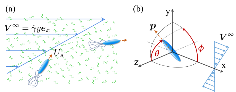
Figure 1: Microswimmers in viscoelastic shear flow. Schematics showing (a) the dilute suspension of microswimmers in an external shear flow $\bm{V}^{\infty}$ of a viscoelastic fluid, (b) coordinate system moving with an individual swimmer that is modelled as an active prolate spheroid of major axis $a$ and minor axis $b$. Here $\bm{p}$ and $U_{s}$ denote the orientation and swimming speed, respectively.

.2 Active spheroid in viscoelastic shear flow

To determine the dynamics of an active spheroid, we first note that a swimmer disturbs the flow field both passively (due to its rigid body) and actively (due to self-propulsion). The disturbance fields are implemented using hydrodynamic multipoles chwang1975hydromechanics ; spagnolie_lauga_2012 . Flagellated microswimmers like E.coli and Chlamydomonas generate a force-dipole flow field and higher order disturbances: source dipole, rotlet dipole, and force quadrupole. We included all four of them and found that only the force-dipole flow field affects the swimmer dynamics in leading order in Wi. The force-dipole field around the active spheroid is $\sigma\frac{\hat{\bm{r}}}{r^{2}}[3(\hat{\bm{r}}\cdot\bm{p})^{2}-1]$ with $\hat{\bm{r}}=\bm{r}/r$. Here, $\sigma$ is a non-dimensional parameter equal to the ratio of the force-dipole strength ($\sigma^{*}$) to the stresslet imposed by the shear flow ($8\pi\mu_{f}\dot{\gamma}l^{3}$), where $\sigma>0$ represents pushers and $\sigma<0$ pullers. For the current work, we focus on swimmers of $5\mu$m size and shear rates of order $0.5-5\text{s}^{-1}$, which corresponds to $\sigma$ of typical wild-type E.coli being roughly $0.04-0.1$ berke2008hydrodynamic ; drescher2010direct . Here, the Weissenberg number can be tuned either by varying the shear rate or relaxation time of the fluid. The latter for the current system is $t_{\text{relax}}\lesssim 0.1s$, which for instance, can be realised in PEO solutions of molecular weight ranging from 2 $-$ 4 $\times 10^{6}$ g mol^-1 and concentration between 0.25 $-$ 0.5 wt$\%$ ebagninin2009rheological . We vary Wi from $0.05-0.5$ by fixing $t_{\text{relax}}$ and changing the shear rates between $\dot{\gamma}\sim 0.5-5\text{s}^{-1}$, following a protocol similar to that for varying $\sigma$.

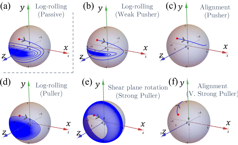
Figure 2: Orientation dynamics of passive $(\sigma=0)$ and active particles in weakly viscoelastic shear flow. The blue curves show time traces of the orientation vector $\bm{p}$ on the unit sphere starting at the red dot. (a) Dipole strength $\sigma=0$, (b) $\sigma=0.06$, (c) $\sigma=0.2$, (d) $\sigma=-0.2$, (e) $\sigma=-0.8$, (f) $\sigma=-2.4$ . Other parameters: Weissenberg number $(\text{Wi})=0.2$, aspect ratio $(\lambda)=5$, initial polar angle $(\theta_{0})=\pi/5$, initial azimuthal angle $(\phi_{0})=\pi/2$, viscometric parameter $\delta=-0.6$. The active and passive viscoelastic coefficients of Eq. (.2) are evaluated to be $\alpha_{1}=4.62$, $\alpha_{2}=-0.33$, $\beta_{1}=0.68$, and $\beta_{2}=1.46$.

In Newtonian fluids, the equation of motion for the orientation $\bm{p}\,(\theta,\phi)$ gives the Jeffery orbits. To formulate this equation for viscoelastic shear, we note that the polymeric stress tensor $\bm{\mathsf{S}}$ is quadratic in the rate-of-strain tensor and vorticity bird1987dynamics . Thus, similar to Einarsson et al. einarsson2015rotation we determine all terms that by symmetry contribute to the rate of change $\dot{\bm{p}}$ up to first order in Wi. Neglecting small terms, we arrive at

$$\dot{\bm{p}} =\left(\bm{\mathsf{I}}-\bm{pp}\right)\cdot\left(\bm{\mathsf{E}}^{\infty}\cdot\bm{p}\right)\left[\Lambda+\text{Wi}\,\sigma\alpha_{1}+\text{Wi}\,\beta_{1}\,\bm{\mathsf{E}}^{\infty}:\bm{pp}\right]$$

$$\;+\bm{\Omega}^{\infty}\times\bm{p}\left[1+\text{Wi}\,\sigma\alpha_{2}+\text{Wi}\,\beta_{2}\,\bm{\mathsf{E}}^{\infty}:\bm{pp}\right]+O(\text{Wi}^{2})$$ (1)

in non-dimensional form, where $\bm{\Omega}$ is the angular velocity and the superscript $\infty$ denotes the quantities that belong to the prescribed shear flow. The shape factor $\Lambda=\frac{-1+\lambda^{2}}{1+\lambda^{2}}$ contains the aspect ratio $\lambda=a/b$, the ratio of major to minor axis. The shape factor approaches $+1$ and $-1$ for needle and disk-like particles, respectively. Since microswimmers are usually elongated, we focus on prolate spheroids of $\Lambda>0.9$, which corresponds to $\lambda>4$; it also helps in simplifying the calculations (see ‘Methods: Hydrodynamic model’). The terms with coefficients $\alpha_{i}$ and $\beta_{i}$ represent the active and passive viscoelastic contributions, respectively. These coefficients are evaluated explicitly as outlined in ‘Methods: Orientation dynamics’ using the Lorentz reciprocal theorem, where we also derive Eq. (.2). For our relevant parameters, we find $\alpha_{1}\gg|\alpha_{2}|$. This along with Eq. (.2) indicates that the modification arising from the activity predominantly depends on the extensional part ($\bm{\mathsf{E}}^{\infty}$) of the viscoelastic shear flow rather than its rotational component. Since the coefficients vary only weakly with $\lambda$ and $\delta$, they are treated as constants in the following discussion of results (see also Supplementary Note 2A).

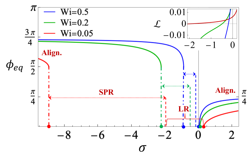
Figure 3: State diagram showing the different states of the orientational dynamics for three Weissenberg numbers. With increasing dipole strength $\sigma$ from left to right, we observe alignment (Align.), shear-plane rotation (SPR), log rolling (LR) and again alignment. In the alignment state, the alignment angle $\phi_{eq}$ is plotted versus dimensionless activity $\sigma$ as solid lines. The dots on the horizontal axis indicate the critical values $\sigma_{c}$ at which alignment (Align.) occurs either to the left of the dashed-dotted lines (pullers, $\sigma<0$) or to the right (pushers, $\sigma>0$). The dashed lines separate SPR and LR from each other at $\sigma=-1.93,\,-0.49,\,-0.19$ for increasing Wi. The inset shows the variation of Lyapunov exponent ($\mathcal{L}$) with $\sigma$. Other parameters are chosen as in Fig. 2.

In the absence of polymers ($\text{Wi}=0$), Eq. (.2) reduces to the well-known Jeffery equation jeffery1922motion that has an infinite number of neutrally stable solutions, i.e., the microswimmer’s orientation traces periodic orbits that depend on initial conditions. During orbital time period $T=2\pi(\lambda+\lambda^{-1})/\dot{\gamma}$, they spent the majority of their time ($\propto\lambda$) aligned near the flow-vorticity plane. When polymers are present, the passive viscoelastic effect breaks the degeneracy of Jeffery orbits and the microswimmer slowly drifts towards an alignment with the vorticity axis, known as the “log-rolling” state gauthier1971_shear-flow ; brunn1977slow ; davino2015particle . Figure 2a shows the curve traced by the orientation of a spheroid on a unit sphere while drifting towards the vorticity axis. This dynamics can be deduced from Eq. (.2) for passive spheroids ($\sigma=0$) when the terms with coefficients $\beta_{1}$ and $\beta_{2}$ are present. In Supplementary Note 2C we also compare our results of passive spheroids with Brunn brunn1977slow .

Now, we illustrate the influence of activity. For weak pushers ($0<\sigma\lesssim 0.1$), the orbits towards log rolling look similar to the ones of passive spheroids, albeit with a larger aspect ratio (see Fig. 2b) since they exhibit more skewed trajectories. This can directly be inferred from Eq. (.2), where activity ($\sigma$) in the term with $\mathrm{Wi}\,\sigma\alpha_{1}$ modifies the shape factor. Since $\alpha_{1}>0$, a pusher ($\sigma>0$) effectively increases $\Lambda$, which corresponds to a higher aspect ratio. The opposite occurs for weak pullers ($\sigma<0$) as they behave like a passive spheroid with reduced aspect ratio. Here the trajectories are more circular as shown in Fig. 2d.

As the dipole strength of a pusher increases beyond a critical value $\sigma_{c}$, the orientation drifts to the shear plane ($\theta=\pi/2$) and aligns at an angle $\phi_{eq}$ with the flow direction (see Fig. 2c). We quantify this transition in Fig. 3 and show that $\sigma_{c}$ (dots close to 0) decreases with increasing ${\rm Wi}$ while $\phi_{eq}$ increases with both $\sigma$ and $\rm{Wi}$. This dynamical behaviour can again be discerned from Eq. (.2), which essentially balances the effect of rotational ($\bm{\Omega}^{\infty}$) and elongational ($\bm{\mathsf{E}}^{\infty}$) flow on $\bm{p}$. Now, activity together with viscoelasticity allows to control this balance. In particular, for our case of $\alpha_{1}\gg|\alpha_{2}|$, we expect the elongational flow to dominate the dynamics for increasing activity. Indeed, when the effective shape factor $\Lambda+\text{Wi}\,\sigma\alpha_{1}$ exceeds unity at a critical value $\sigma_{c}$, the dynamics of $\bm{p}$ transitions from the orbital to the alignment state as favored by the elongational flow. In ‘Methods: Dynamical analysis 1’, we show for a modified dynamical system that the relevant eigenvalue of the dynamical matrix becomes real at $\sigma_{c}$, as expected for such a transition, and the corresponding eigenvector gives the alignment angle $\phi_{eq}$. As $\sigma$ increases, $\phi_{eq}$ grows from zero and approaches $\pi/4$ for large $\sigma$, since in this limit, the elongational flow ($\bm{\mathsf{E}}^{\infty}$) with its principal axis along $\phi=\pi/4$ completely dominates the dynamics of $\bm{p}$.

For pullers, Fig. 2e shows that increasing the activity induces a transition from log rolling towards rotation in the shear plane. This orbit is also observed for passive particles with oblate shape ($\Lambda<0$) in viscoelastic flows (gauthier1971_shear-flow, ; brunn1977slow, ; davino2015particle, ). It appears here and acts as an attracting limit cycle, when the effective shape factor $\Lambda+\text{Wi}\sigma\alpha_{1}$ in Eq. (.2) becomes negative due to the puller activity $\sigma<0$. We have performed a stability analysis for the shear-plane rotation in ‘Methods: Dynamical analysis 2’ and calculated the Lyapunov stability exponent $\mathcal{L}$. It determines the exponential time variation of the disturbed limit cycle. In the inset of Fig. 3, we show the Lyapunov exponent as a function of $\sigma$. For weak and moderate pullers, $\mathcal{L}>0$ shows that shear-plane rotation is an unstable limit cycle, where the system drifts towards stable log rolling. As the dipole strength of the puller becomes more negative, $\mathcal{L}$ turns negative meaning that shear-plane rotation is stable. Upon analysing the orbital dynamics in the shear-plane rotation, we find that increasing $|\sigma|$ gradually slows down the swimmer’s rotation near the $y$-axis, along which the flow gradient is applied. Eventually, a transition to permanent alignment with $\phi_{eq}=\pi/2$ occurs, which can be similarly analyzed as the alignment transition of pushers. However, here it occurs at the effective shape factor $\Lambda+\text{Wi}\,\sigma_{c}\alpha_{1}=-1$. With further increasing $|\sigma|$ the active spheroid tilts against the flow, in contrast to pushers, and asymptotes at $3\pi/4$, which is the direction of the second principal axis of the elongational flow ($\bm{\mathsf{E}}^{\infty}$). This behavior is illustrated in Fig. 2f and Fig. 3. Finally, Fig. 3 also shows that as Wi increases, the regime of shear-plane rotation shrinks.

.3 Impact of noise on orientational dynamics

The deterministic orientational dynamics is disturbed by two types of stochastic reorientations of the swimming direction, which we now address with the help of the Smoluchowski equation. First, a bacterium tumbles, which is triggered when the rotation of one of its flagella reverses so that it leaves the flagellar bundle berg1983random ; lauga2016bacterial ; adhyapak2016dynamics . For a wild type E.coli, tumbling occurs roughly every $1\mathrm{s}$, where it attains a new random orientation. Although tumbling is biased in the forward direction with a mean tumbling angle of roughly $68.5^{\circ}$, we model it to be unbiased for computational ease because it only affects our results marginally as suggested by Nambiar et al. nambiar2017stress . Second, thermal rotational diffusion continuously reorients a microswimmer but its effect is small compared to tumbling.

We now evaluate the orientational distribution of an ensemble of non-interacting microswimmers in steady state, caused by the three mechanisms discussed so far: deterministic motion in background shear flow, tumbling, and rotational diffusion. The steady-state probability distribution function $\psi(\bm{p})$ for the orientation vector of non-interacting microswimmers is governed by the Smoluchowski equation doi1988theory

$$\text{Pe}_{f}\nabla_{p}\cdot\left(\bm{\dot{p}}{\psi}\right)-\tau D_{r}\nabla_{p}^{2}{\psi}+\left({\psi}-\frac{1}{{4\pi}}\right)=0,$$ (2)

where $\psi(\bm{p})$ is normalized to unity. The first term describes the orientational drift using $\nabla_{p}$ as the gradient operator on the unit sphere. To compare the strength of flow-induced reorientation to the mean time $\tau$ between two tumbling events, we introduce the flow Péclet number $\mathrm{Pe}_{f}=\dot{\gamma}\tau$. Tumbling away from the swimming direction $\bm{p}$ is handled by the third term and rotational diffusion by the second term. For bacteria, the latter is typically small compared to tumbling since $\tau\sim 1\mathrm{s}$ berg1983random and $D_{r}\lesssim 0.1\mathrm{s}^{-1}$, as an estimate from the Stokes-Einstein relation shows. In restricting ourselves to Eq. (2), we assume a spatially uniform system valid when hydrodynamic and steric interactions with bounding surfaces can be neglected spagnolie_lauga_2012 ; spagnolie2022swimming . In particular, this means that the mean length of persistent swimming, $U_{s}\tau$, where $U_{s}$ is the swimming speed, is much smaller than the spatial extent of the system. Finally, we consider weak fluid elasticity with relaxation time $t_{\mathrm{relax}}\ll\tau,D_{r}^{-1}$, so that the fluid relaxes faster than the time scales given by stochastic reorientations cohen1987orientation . Typical dilute and semi-dilute PEO solutions of molecular weight of $\sim 10^{6}$ g mol^-1 have $t_{\text{relax}}\lesssim 0.1$s ebagninin2009rheological , whereas the stochastic reorientation time scale is always $1$s or larger. Thus, here we do not need to take into account any memory in the rotational noise.

In the following, we want to emulate a rheological experiment and vary the shear rate $\dot{\gamma}$ via $\text{Pe}_{f}$, while the fluid and swimmer properties are kept constant. Therefore, in Eq. (.2) for the rotational drift velocity $\dot{\bm{p}}$, we rewrite Wi as $\text{Pe}_{f}\text{De}$, where the Deborah number $\text{De}=t_{\mathrm{relax}}/\tau$ compares the fluid relaxation time to $\tau$. Furthermore, the second relevant parameter, $\text{Wi}\sigma$, does not explicitly depend on $\dot{\gamma}$ but rather quantifies the strength of activity relative to fluid elasticity. To vary the activity independent of other parameters, we replace $\text{Wi}\sigma$ by $\text{Pe}_{a}\text{De}/8\pi$. Here, ${\rm Pe}_{a}$ is the signed activity Peclet number that is positive for pushers and negative for pullers. Using $U_{s}\sim\sigma^{*}/(\mu_{f}l^{2})$ for the swimming speed with the force dipole moment $\sigma^{*}$berke2008hydrodynamic , we can write it in the familiar form ${\rm Pe}_{a}\sim U_{s}\tau/l$. Thus, its magnitude compares the persistence length to the body length $l$. A wild-type E.coli typically has $\text{Pe}_{a}\lesssim 5$ berg1983random ; chattopadhyay2006swimming . We numerically solve Eq. (2) for arbitrary $Pe_{f}$ by expanding $\psi$ in spherical harmonics and taking into account the first 100 harmonics. The numerical solution is also verified analytically in the limit of $\text{Pe}_{f}\ll 1$ (see further details in ‘Methods: Kinetic model’).

Figure 4 shows the orientational probability distribution of passive and active particles for various cases. It quantifies the orientational ‘microstructure’ of a suspension of non-interacting and orientable particles subject to shear flow hinch1976constitutive ; chen1996rheology ; nambiar2017stress . We begin with discussing the case of weak shear rate ($\text{Pe}_{f}<1$) in Figs. 4a-d. In the absence of shear flow, the microstructure is solely governed by rotational noise and is therefore isotropic. For weak shear rates the extensional part ($\bm{\mathsf{E}}^{\infty}$) of the shear flow primarily distorts the microstructure, which peaks near the extensional axis as noted for Newtonian fluids by Hinch and Leal hinch1972effect . We quantify this in ‘Methods: Kinetic model 1’ by solving Eq. (2) via a perturbation expansion in $\text{Pe}_{f}$ and obtain the first-order correction:

$$\psi_{(1)}=\frac{3}{4\pi}(\Lambda+\alpha_{1}\text{De}\text{Pe}_{a}/8\pi)\frac{\bm{\mathsf{E}}^{\infty}:\bm{p}\bm{p}}{1+6\tau D_{r}}$$ (3)

In the absence of activity, there is no deviation from the Newtonian microstructure at this order.

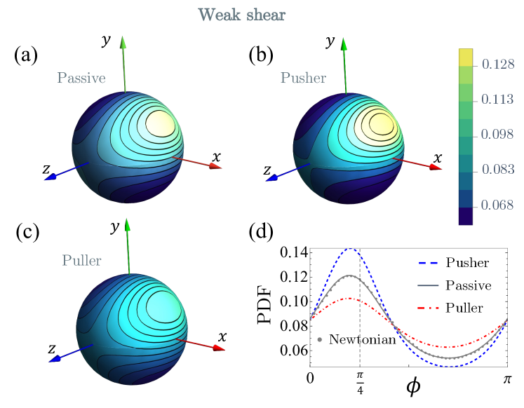
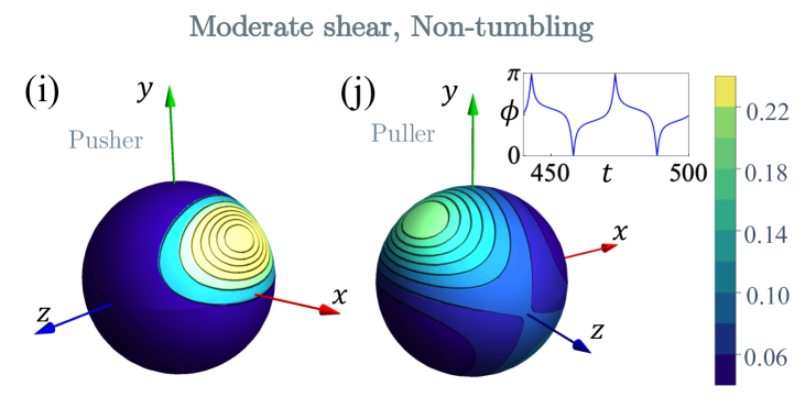
Figure 4: Orientational probability distribution $\psi(\bm{p})$ for (a-d) weak shear flow at flow Péclet number $\text{Pe}_{f}=0.5$, (e-j) moderate shear flow at $\text{Pe}_{f}=5$. The activity Péclet number ($\text{Pe}_{a}$) varies as (a,e) $\text{Pe}_{a}=0$, (b,f) $\text{Pe}_{a}=20$, (c,g) $\text{Pe}_{a}=-20$ and always with $D_{r}\tau=0.1$, where $\tau$ is tumbling time and $D_{r}$ is the rotary diffusion coefficient. (d,h) Probability distribution function (PDF) in the flow-shear plane; the inset in (h) shows PDF in the flow-vorticity plane. Non-tumbling particles: (i) $\text{Pe}_{a}=100$, (j) $\text{Pe}_{a}=-100$. The insets in (e,g,j) show the polar angle $\phi(t)$ for the shear-plane rotation state corresponding to the respective distributions. Colour bars indicate the value of PDF. Other parameters are chosen as in Fig. 2 with Deborah number $\text{De}={t_{\text{relax}}/\tau}=0.1$. To locate these distributions in Fig.  3, we give the corresponding Weissenberg and activity numbers: (a-d) $\text{Wi}=0.05$, $\sigma=\pm 1.6$; (e-h) $\text{Wi}=0.5$, $\sigma=\pm 0.16$; (i,j) $\text{Wi}=0.5$, $\sigma=\pm 0.8$.

In Figs. 4a-d we use a weak shear rate of $\text{Pe}_{f}=0.5$ and $|\text{Pe}_{a}|=20$, which is an activity close to mutated strains of tumbling E. coli (pusher) wolfe1988acetyladenylate and the algae C. reinhardtii (puller). The observed distributions follow the trend of Eq. (3). While pushers ($\text{Pe}_{a}>0$) enhance the alignment along the extensional axis of the applied shear flow, pullers ($\text{Pe}_{a}<0$) weaken it. We note that the peak of the orientational distributions in the shear plane (plot d) exhibits a small deviation from $\phi=\pi/4$. This is due to the rotational flow ($\bm{\Omega}^{\infty}$), which contributes to $\psi(\bm{p})$ in second order in $\text{Pe}_{f}$ chen1996rheology .

As the shear rate increases, the deterministic dynamics becomes more visible. We illustrate this in Figs. 4e-h for $\text{Pe}_{f}=5$. Compared to Fig. 4a, the peak in $\psi(\bm{p})$ for passive particles (Fig. 4e) shifts towards the flow axis and becomes more anisotropic along the flow-vorticity plane, as the deterministic velocity $\dot{\bm{p}}$ is smallest in this plane. Eventually, $\dot{\bm{p}}$ approaches zero in the deterministic log-rolling state observed in viscoelastic fluids (Fig. 2a). However, the deterministic log-rolling state is not completely reflected in the distribution because the slow relaxation towards the vorticity axis is always interrupted by the dominating stochastic reorientations (see Supplementary note 4, where we illustrate the orientation distribution for a larger weakly Brownian particle that resembles log-rolling). Note that due to the fluid elasticity, the peak of $\psi(\bm{p})$ in Fig. 4h is slightly closer to the flow axis compared to the Newtonian case. Furthermore, the inset therein also illustrates a broader distribution in the flow-vorticity plane ($\phi=0$). Further increasing $\text{Pe}_{f}$ spreads the distribution even more in the flow-vorticity plane and, ultimately, for $\text{Pe}_{f}\gtrsim 100$ the peak develops along the vorticity axis, which is entirely reminiscent of log rolling. However, this is a regime which we cannot strictly capture as our analysis requires De, $\text{Wi}<1$, which means $\text{Pe}_{f}<10$. These findings are qualitatively consistent with earlier studies on passive fibre suspensions at moderate shear rates (cohen1987orientation, ; chung1987orientation, ) (further illustrated in Supplementary Note 4).

Figure 4f demonstrates that the activity of pushers in conjunction with the higher shear rate ($\text{Pe}_{f}=5$) makes the distribution more anisotropic. According to Fig.4h, pushers strongly focus at an angle $\phi=18^{\circ}$ in comparison to a weaker peak of passive particles near to flow axis. This angle is close to the alignment angle $\phi_{eq}=21^{\circ}$ of the deterministic state with the parameters $\text{Wi}=0.5$, $\sigma=0.16$ in Fig. 3. Conversely to pushers, pullers reduce the anisotropy in the orientational distribution as shown in Fig.4g. We can directly relate this observation to the deterministic velocity $\dot{\bm{p}}$ with parameters $\text{Wi}=0.5$, $\sigma=-0.16$ that indicate again the log-rolling state; the resulting orbit is similar to that depicted in Fig. 2d. Compared to the passive case, the orbit is more circular, which we already related to a reduced effective aspect ratio when discussing the deterministic orientational dynamics. Therefore, the orientation is less constrained to the flow-vorticity plane. This is explained by the dynamics of the azimuthal angle $\phi$ in the inset of Fig. 4g that shows lesser time spent in the plane compared to the inset in Fig. 4e. As a result, the distribution is broader and less anisotropic (leal1971effect, ). Consequently, the particle is less susceptible to the effect of stochastic reorientations and thus, its distribution has a peak closer to the flow axis. Hence, unlike active Newtonian suspensions saintillan2010dilute , the microstructure of microswimmers in a viscoelastic fluid is clearly sensitive to their hydrodynamic signature being either pushers or pullers.

We also examined the orientational distributions of microswimmers that do not tumble and only experience rotational thermal noise. Therefore, in this case we eliminate the last term on the right-hand side of Eq. (2) and redefine our parameters $\text{Pe}_{f}$, $\text{Pe}_{a}$, and De replacing $\tau$ by $D_{r}^{-1}$. For passive particles and activity $\text{Pe}_{a}\sim O(10)$, the microstructure is qualitatively similar to the distributions in Figs. 4a-h. However, microswimmers that do not tumble can have larger persistence lengths elgeti2015physics . In particular, one can genetically modify E.coli such that tumbling does not occur berke2008hydrodynamic ; junot2019swimming ; wolfe1988acetyladenylate . Therefore, in Figs. 4i and j we show the orientational distributions for $\text{Pe}_{a}=\pm 100$. Compared to Fig. 4f, increasing the activity of a pusher moves the peak in the distribution function (at $\phi=34^{\circ}$) even closer to the alignment angle ($\phi_{\text{eq}}=36^{\circ}$) of the deterministic alignment state. For pullers we observe an even more drastic change upon increasing the activity. The peak in the orientational distribution shifts to the quadrant where the compressional part of the shear flow occurs (see Fig. 4j). Interestingly, this is not due to the deterministic alignment of pullers as the parameters ($\text{Wi}=0.5,\,\sigma=-0.8$) belong to the shear-plane rotation state (see Fig. 3). As already explained in the discussion of Fig. 3, the rotational velocity $\dot{\bm{p}}$ slows down near $\phi=\pi/2$ when the effective shape factor $\Lambda+\text{Wi}\,\sigma_{c}\alpha_{1}$ becomes negative. Therefore, the active particle resembles a passive oblate spheroid brown2000orientational . Indeed, the inset of Fig. 4j shows how the puller orientation spends more time near $\phi=\pi/2$. This again shows that even in the presence of significant noise the microstructure is determined by the deterministic dynamics.

.4 Shear viscosity of active suspensions

Finally, we evaluate the effective shear viscosity of a dilute active suspension from the total stress tensor, $\bm{\mathsf{\Sigma}}=\bm{\mathsf{\Sigma}}_{f}+\bm{\mathsf{\Sigma}}_{p}$, where subscripts $f$ and $p$ refer to fluid and particle contributions, respectively. The deviatoric component of $\bm{\mathsf{\Sigma}}$ provides the shear viscosity, $\mu=\mu_{f}+\varphi\mu_{p}$, where $\varphi\mu_{p}=\Sigma_{p\,xy}/\dot{\gamma}$ is due to the suspended microswimmers and $\varphi=na^{3}$ is proportional to their volume fraction with $n$ being the particle density. Note that the shear viscosity $\mu_{f}$ of the second-order fluid does not depend on the shear rate, while $\mu_{p}$ is dependent on it. To evaluate $\mu_{p}$, we need to average over the stresslets $\bm{\mathsf{\Pi}}(\bm{p})$ generated by the suspended particles. Using the orientational distribution, we obtain

$$\bm{\mathsf{\Sigma}}_{p}=n{\langle{\bm{\mathsf{\Pi}}}\rangle}=n\int_{S}\bm{\mathsf{\Pi}}(\bm{p})\psi(\bm{p})\text{d}\bm{p},$$ (4)

where $\bm{\mathsf{\Pi}}(\bm{p})$ is the sum of three contributions saintillan2010dilute , which give the following stress tensors: $\bm{\mathsf{\Sigma}}^{A}_{p}=n\sigma^{*}\left[{\langle{\bm{pp}}\rangle}-\bm{\mathsf{I}}/3\right]/8\pi$ due to activity, $\bm{\mathsf{\Sigma}}^{T}_{p}=3nk_{B}T\left[{\langle{\bm{pp}}\rangle}-\bm{\mathsf{I}}/3\right]$ due to thermal reorientations batchelor1970 , and $\bm{\mathsf{\Sigma}}^{F}_{p}$ due to the resistance of passive particles to shear. For Newtonian fluids, the latter was first derived by Einstein einstein1906new for spherical particles, and then later generalized to elongated particles by Hinch and Leal hinch1975constitutive ; hinch1976constitutive . For the second-order fluid, we follow Férec et al. ferec2017steady and approximate it using the Geisekus form, $\bm{\mathsf{\Sigma}}^{F}_{p}=-\mu_{f}nl^{3}A\dot{\gamma}\overset{\nabla}{{\langle{\bm{pp}}\rangle}}/2$, where $A=\pi/6\ln(2\lambda)$ is a shape factor to access the friction of a long slender body and $\overset{\nabla}{{\langle{\bm{pp}}\rangle}}$ is the upper-convected time derivative of the second moment of $\psi(\bm{p})$. The expression for $\bm{\mathsf{\Pi}}^{F}$ was originally derived for dumbbells suspended in a Newtonian fluid birdTWO1987dynamics . As in Ref. ferec2017steady , we use it here as an approximation for the stress response of particles in a weakly viscoelastic fluid, as there are no closed form expressions available. The consequences of the second-order fluid come in through the orientational dynamics $\dot{\bm{p}}$ in Eq. (.2) and further terms in the upper-convected derivative (see ‘Methods: Rheology’). The expressions for the three contributions to the particle stress tensor are pertinent to studies on slender rods and fibres (i.e., $\Lambda\to 1$), and henceforth, we will be focusing on spheroids with larger aspect ratios ($\lambda=10$). Using Eq. (4) in the definition of the particle-induced contribution to shear viscosity, $\varphi\mu_{p}=\Sigma_{p\,xy}/\dot{\gamma}$, together with our characteristic parameters, we obtain

$$\frac{\mu_{p}}{\mu_{f}}=-4A\overset{\nabla}{{\langle{\bm{pp}}\rangle}}_{xy}+\frac{8}{\text{Pe}_{f}}\left(6\tau D_{r}A-\frac{\text{Pe}_{a}}{8\pi}\right)\left[{\langle{\bm{pp}}\rangle}-\frac{\bm{\mathsf{I}}}{3}\right]_{xy}.$$ (5)

We use numerical solutions of Eq. (2) for the orientational distribution $\psi(\bm{p})$ to evaluate $\mu_{p}$ for varying $\mathrm{Pe}_{f}$ and $\mathrm{Pe}_{a}$. We also match the numerical values of $\mu_{p}$ with an expression, which we obtain using the analytic form of $\psi(\bm{p})$ from Eq. (3) in the limit of small $\text{Pe}_{f}$ (the derivation is provided in ‘Methods: Rheology’). In Supplementary Figure 4, we also show that our results agree with Saintillan saintillan2010dilute in the Newtonian limit.

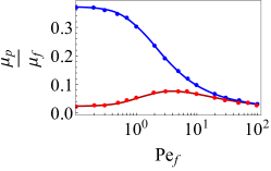
Figure S4: Comparing the shear viscosity as a function of $\text{Pe}_{f}$ from our analysis in the Newtonian fluid limit with that of Ref. saintillan2010dilute for $\frac{|\text{Pe}_{a}|}{8\pi A}=1$, $\Lambda=1$, $\tau=1$, $D_{r}=0.1$. Lines (blue is puller, red is pusher) indicate our viscosity ratio and dots correspond to Ref. saintillan2010dilute , whose viscosity is defined here with respect to the particle volume fraction $\varphi=na^{3}$. Ref. saintillan2010dilute used $\varphi=nl^{3}A$.

Figure S4a shows the particle-induced contribution to shear viscosity normalized by the bare fluid viscosity $\mu_{f}$, which is plotted versus shear strength $\text{Pe}_{f}$. We begin with discussing suspensions in a Newtonian fluid (dashed lines) saintillan2010dilute . When a suspension of passive rods (black) is sheared weakly ($\text{Pe}_{f}\ll 1$), the orientational microstructure is governed by Eq. (3) with $\text{De}=0$ and resembles Fig. 4a. Here, the rods are aligned along the extensional axis of the applied shear flow and resist shearing ($\mu_{p}>0$), which enhances viscosity. For a suspension of pushers (brown dashed) in the weak-shear regime, the microstructure still resembles Fig. 4a, but now the extensile force dipoles support the elongational part of the shear flow, which results in $\mu_{p}<0$ so that the total shear viscosity is smaller than $\mu_{f}$. Conversely, pullers (green dashed) with their contractile force dipoles additionally resist shear flow and thereby enhance viscosity. Note that, since the microstructure of active suspensions in a Newtonian fluid is unchanged by the hydrodynamic signature of microswimmers, the magnitude of the activity contribution to $\mu_{p}$ is identical for pushers and pullers. As the shear rate increases, the magnitude of $\mu_{p}$ for both passive and active rods reduces, which resembles a typical shear-thinning/thickening behaviour. For passive particles the microstructure is similar to Fig. 4e. The alignment close to the flow axis explains why the resistance of particles to the applied shear flow is reduced. For active particles, the activity-induced flow becomes less and less important with increasing shear rate as quantified by the inverse proportionality to $\text{Pe}_{f}$ in Eq. (5).

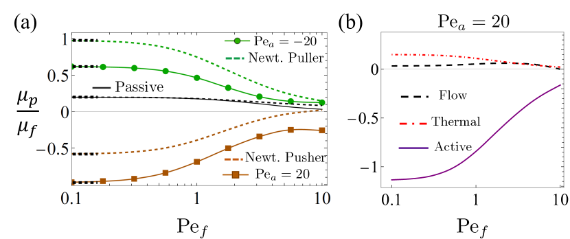
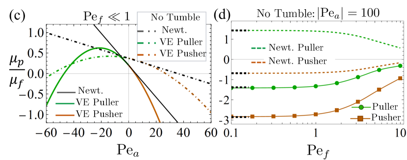
Figure 5: Particle-induced contribution to viscosity $\mu_{p}/\mu_{f}$ in a weakly viscoelastic (VE) fluid: (a) plotted vs. shear rate (characterized by the flow Péclet number $\text{Pe}_{f}$) for pusher ($\text{Pe}_{a}>0$), puller ($\text{Pe}_{a}<0$), and a passive rod ($\text{Pe}_{a}=0$) with solid lines. Dashed lines correspond to the Newtonian case. (b) Contributions to particle-induced viscosity for activity Péclet number $\text{Pe}_{a}=20$. (c) $\mu_{p}/\mu_{f}$ vs. activity $\text{Pe}_{a}$ in the $\text{Pe}_{f}\ll 1$ limit for tumbling and non-tumbling active rods. (d) $\mu_{p}/\mu_{f}$ vs. shear rate $\text{Pe}_{f}$ for non-tumbling active rods with large persistence length, $|\text{Pe}_{a}|=100$. Dotted black lines near $\text{Pe}_{f}=0.1$ in (a,d) correspond to the analytical results for $\text{Pe}_{f}\ll 1$. Other parameters: Deborah number $\text{De}=0.1$, the active and passive viscoelastic coefficients of Eq. (.2) are evaluated to be $\alpha_{1}=5.92,\;\alpha_{2}=-0.91,\;\beta_{1}=0.63,\;\beta_{2}=1.18$ for aspect ratio $\lambda=10$.

Now, we discuss the results for the second-order fluid (SOF) in Fig. S4a (solid lines). For the suspension of passive rods (black), we do not find an appreciable deviation from the Newtonian case until $\text{Pe}_{f}\approx 10$, similar to Refs. cohen1987orientation ; chung1987orientation . However, for active suspensions the modifications are substantial and qualitatively different for pushers (brown) and pullers (green). For pushers, the reduction in viscosity is further enhanced compared to Newtonian fluids, whereas the viscosity enhancement of pullers is reduced. For a fixed viscosity of $\mu_{f}$ and a volume fraction of $\varphi=0.1$, a pusher suspension of $\text{Pe}_{a}=20$ predicts a $10\%$ viscosity reduction, whereas in a Newtonian fluid the reduction is $6\%$. We understand this viscosity reduction by using the orientational distributions in Fig. 4: pushers are even more aligned in the extensional quadrant of the applied shear flow (Fig. 4b,d,f), which explains their further increased support of shear flow. In contrast, pullers are less aligned compared to the Newtonian case (Fig. 4c,d,g) and, therefore, oppose the shear flow to a reduced extent. Figure S4b for pushers clearly shows that the active stress ($\bm{\mathsf{\Sigma}}^{A}$) dominates and hence is primarily responsible for the observed viscous response.

In the limit of shear rate much smaller than tumbling rate, $\text{Pe}_{f}\ll 1$ , we can calculate $\mu_{p}/\mu_{f}$ analytically using Eq. (3) (see ‘Methods: Rheology’) and obtain:

$$\frac{\mu_{p}}{\mu_{f}}= \frac{4A(5-3\Lambda)}{15}+\frac{48A\tau D_{r}-\text{Pe}_{a}/\pi}{5\left(1+6\tau D_{r}\right)}\left(\Lambda+\frac{\text{De}\,\text{Pe}_{a}\alpha_{1}}{8\pi}\right)$$

$$-\frac{\text{De}\,\text{Pe}_{a}A\alpha_{1}}{10\pi}.$$ (6)

We elaborate the result here since the influence of passive and active rods on the shear viscosity is the strongest in this limit. In Fig. S4c we plot $\mu_{p}/\mu_{f}$ vs. $\text{Pe}_{a}$ for tumbling microswimmers (solid lines). As Eq. (.4) shows, elasticity in the fluid adds a quadratic dependence in $\text{Pe}_{a}$, while in a Newtonian fluid the dependence is only linear saintillan2010dilute . For all $\text{Pe}_{a}$, except a small region close to $\text{Pe}_{a}=0$, the values of $\mu_{p}/\mu_{f}$ remain below those obtained in the Newtonian limit. Thus, fluid elasticity reduces the shear viscosity for both pusher and puller suspensions. Note that, as we increase the activity of pullers ($\text{Pe}_{a}\lesssim-50$), they too can reduce the shear viscosity ($\mu_{p}/\mu_{f}<0$) like pushers. This is a consequence of the orientational distribution shown in Fig. 4j; pullers with large activity align preferentially in the compressional quadrant of the shear flow and thereby also support the shearing fluid similar to pushers aligned in the extensional quadrant.

As described earlier, we can treat the case of non-tumbling microswimmers by replacing $\tau$ by $D_{r}^{-1}$ in the definitions of $\text{Pe}_{f}$, $\text{Pe}_{a}$, and De. With these parameters, Eq. (.4) can be formulated in the limit $\tau\rightarrow\infty$ to show that the viscosity contribution of non-tumbling active rods also follows a quadratic dependence in $\text{Pe}_{a}$ (Fig. S4c, dashed lines). Non-tumbling microswimmers can exhibit high persistence lengths. Thus, in Fig. S4d we show for $|\text{Pe}_{a}|=100$ that their contribution to viscosity is negative over a wide range of shear rates for both pushers and pullers in a second-order fluid. Hence, we find that the elasticity of a fluid always results in a reduced total viscosity as compared to suspensions in a Newtonian fluid of identical base viscosity ($\mu_{f}$).

Discussion

In this article we show how activity influences the dynamics of a sheared microswimmer suspension in a viscoelastic fluid at an individual level and in the bulk. At the individual level, the orientational dynamics of passive rods is well known from Jeffery’s orbits in Newtonian shear jeffery1922motion and ‘log-rolling’ orbits in viscoelastic shear flow leal1975slow ; brunn1977slow . Our analytical result [Eq. (.2)], derived for elongated active spheroids in a second-order fluid, demonstrates how the active flow field of a swimmer modifies the orientational dynamics. Extensile swimmers like E.coli (pushers) drift to the shear plane and align at an angle to the flow direction. For contractile swimmers like C. reinhardtii (pullers), activity effectively lowers their aspect ratio. With increasing dipole strength, pullers show log rolling, transition to shear-plane rotation, and ultimately align at an angle against the flow direction. The latter occurs for strong pullers at dipole strengths relevant to artificial swimmers with large propulsion speed ren20193d ; aghakhani2020acoustically .

To demonstrate the impact of the individual swimmer dynamics on the bulk rheological behaviour, we employ the Smoluchowski equation to evaluate the orientational probability distribution of an ensemble of active spheroids called the suspension microstructure hinch1975constitutive . Accounting for tumbling and rotary diffusion, we find that the microstructure is sensitive to the hydrodynamic signature of the swimmer unlike suspensions in Newtonian fluids hatwalne2004rheology ; saintillan2010dilute ; nambiar2017stress . Pushers align more strongly in the extensional quadrant of the applied shear flow, while the alignment of pullers is significantly weaker. This activity-specific microstructure significantly modifies the effective shear viscosity compared to Newtonian fluids lopez2015turning . In particular, the viscosity reduction of a dilute pusher suspension is more pronounced under viscoelastic shear flow, while the viscosity enhancement of pullers is weaker. Thus, the activity of a microswimmer contributes in two ways to the rheology of swimmer suspensions in a viscoelastic fluid; directly through its active stresses and indirectly by coupling to the elasticity of the fluid and thereby influencing the orientational microstructure. In particular, in the weak-shear limit the particle-induced contribution to viscosity scales quadratically with the activity $\text{Pe}_{a}$. In total, we find that the elasticity of a second-order fluid always reduces the total viscosity of the microswimmer suspension, as compared to a Newtonian fluid of identical base viscosity. Especially for pushers, this might help to reach the regime of superfluidity at lower volume fractions compared to Newtonian fluids. We note that superfluidity is reported to be also associated with onset of collective motion guo2018symmetric ; aranson2022bacterial , and requires further analysis at higher microswimmer densities.

Most biological fluids are viscoelastic. We presented a first systematic study of the individual dynamics and the bulk rheology of microswimmers suspended in such fluids. Earlier investigations on active suspensions in quiescent bozorgi2011effect and vortical viscoelastic flows ardekani2012emergence assumed conventional Newtonian Jeffery orbits. In the light of our results, these studies on the collective behaviour might need to be revisited. Our investigations makes several assumptions to address the complexity of microbial flows, which offers ample opportunities for future developments. Biological fluids can be more complex and exhibit shear-thinning/-thickening properties or several characteristic relaxation times, which requires more evolved modeling using, for example, the FENE-P or Giesekus model. Furthermore, mucus besides being significantly shear-thinning has relaxation times larger than 1 second, which is of the order of the bacterial mean free tumble time li2021microswimming ; spagnolie2022swimming ; mucus_lai2009micro . Thus, noise becomes non-Markovian and memory needs to be incorporated in the stochastic description, for example, within a generalized Langevin equation narinder2018memory .

Methods

.1 Hydrodynamic Model

The hydrodynamics around the spheroidal particle is governed by the mass and momentum conservation as $\nabla\cdot\bm{V}=0,\;\nabla\cdot\bm{\mathsf{T}}=0.$ Here $\bm{\mathsf{T}}$ is the total stress tensor defined as $\bm{\mathsf{T}}=-P\,\bm{\mathsf{I}}+2\,\bm{\mathsf{E}}+\text{Wi}\,\bm{\mathsf{S}}$ bird1987dynamics , where $\bm{\mathsf{S}}=4\bm{\mathsf{E}}\cdot\bm{\mathsf{E}}+2\delta\overset{\Delta}{\bm{\mathsf{E}}}$. The lower-convected derivative is defined as

$$\overset{\Delta}{\bm{\mathsf{E}}}=\left[\frac{\partial\bm{\mathsf{E}}}{\partial t}+\left(\bm{V}\cdot\bm{\nabla}\right)\bm{\mathsf{E}}+\bm{\mathsf{E}}\cdot\bm{\nabla}\bm{V}+\bm{\nabla V}^{T}\cdot\bm{\mathsf{E}}\right]\,.$$ (7)

Since we consider a steady shear flow and a steadily active swimmer, we can disregard the temporal derivative in the above stress tensor. In particle frame of reference, the boundary condition on its surface is the no-slip condition $\bm{V}=\bm{\Omega}^{p}\times\bm{r}$, where the rotational velocity $\bm{\Omega}^{p}$ is currently unknown and will be evaluated by using the torque-free condition. We split the velocity field into the disturbance field $\bm{v}$ and background flow field $\bm{V}^{\infty}=\bm{\mathsf{E}}^{\infty}\cdot\bm{r}+\bm{\Omega}^{\infty}\times\bm{r}$ i.e., $\bm{V}=\bm{v}+\bm{V^{\infty}}$. The equations governing the disturbance flow field are

$$\nabla\cdot\bm{v} = 0,\quad-\nabla p+\nabla^{2}\bm{v}=-\text{Wi}\,(\nabla\cdot\bm{\mathsf{s}}),\text{ where}$$

$$\bm{\mathsf{s}} = 4(\bm{\mathsf{e}}\cdot\bm{\mathsf{e}}+\bm{\mathsf{w}})+2\,\delta(\overset{\Delta}{\bm{\mathsf{e}}}+\overset{\Delta}{\bm{\mathsf{w}}}).$$ (8)

Here $\bm{\mathsf{e}}$ is the rate of strain tensor for the disturbance flow $(\nabla\bm{v}+\nabla\bm{v}^{\dagger})/2$, whereas $\bm{\mathsf{w}}$, $\overset{\Delta}{\bm{\mathsf{e}}}$ and $\overset{\Delta}{\bm{\mathsf{w}}}$ are the different constituents of the polymeric tensor ($\bm{\mathsf{s}}$) due to the disturbance flow field. Specifically, $\bm{\mathsf{w}}$ is the interaction tensor defined as $\bm{\mathsf{E}}^{\infty}\cdot\bm{\mathsf{e}}+\bm{\mathsf{e}}\cdot\bm{\mathsf{E}}^{\infty}$, arising from the interaction between background flow and disturbance field; and $\overset{\Delta}{\bm{\mathsf{w}}}$ is the lower-convected derivative of $\bm{\mathsf{e}}$ and $\bm{\mathsf{E}}^{\infty}$ with respect to $\bm{V}^{\infty}$ and $\bm{v}$, respectively:

$$\overset{\Delta}{\bm{\mathsf{w}}}={\bm{V}^{\infty}}\cdot\nabla\bm{\mathsf{e}}+\bm{\mathsf{e}}\cdot\nabla{\bm{V}^{\infty}}^{\dagger}+\nabla{\bm{V}^{\infty}}\cdot\bm{\mathsf{e}}$$ (9)

$$\qquad\qquad\qquad+\bm{v}\cdot\nabla\bm{\mathsf{E}}^{\infty}+\bm{\mathsf{E}}^{\infty}\cdot\nabla\bm{v}^{\dagger}+\nabla\bm{v}\cdot\bm{\mathsf{E}}^{\infty}.$$

The boundary conditions of the disturbance field at the particle surface and far away are

$$\bm{v}=\Delta\bm{\Omega}\times\bm{r}-\bm{\mathsf{E}}^{\infty}\cdot\bm{r}\quad\mbox{at\ }\bm{r}\in S\quad\text{and}\quad\bm{v}\to\bm{0}\quad\mbox{as\ }\;\bm{r}\to\infty,$$ (10)

respectively. Here $\Delta\bm{\Omega}$ is the difference in particle angular velocity and background vorticity ($\bm{\Omega}^{p}-\bm{\Omega}^{\infty}$).

For small values of Wi, the disturbance field variables are expanded as $f=f^{(0)}+\text{Wi}\;f^{(1)}+\cdots.$ Here, $f$ is a generic field variable that represents velocity ($\bm{v}$), pressure ($p$), and angular velocity ($\bm{\Omega}^{p}$). We substitute this expansion in the Eq. (.1) and obtain the $O(1)$ Stokes problem as

$$\nabla\cdot\bm{v}^{(0)} = 0,\quad-\nabla p^{(0)}+\nabla^{2}\bm{v}^{(0)}=0$$ (11)

with the boundary condition at particle surface:

$$\bm{v}^{(0)}=\Delta\bm{\Omega}^{(0)}\times\bm{r}-\bm{\mathsf{E}}^{\infty}\cdot\bm{r}\quad\mbox{at\ }\bm{r}\in S,$$ (12)

and a decaying condition at infinity ($\bm{v}^{(0)}\to 0$). Using the finite multipole expansion around the spheroid chwang1975hydromechanics ; einarsson2015rotation ; abtahi2019jeffery , we obtain the disturbance velocity for a passive spheroid at $O(1)$ as

$$v^{(0)}_{i} =\mathcal{Q}_{ij,k}^{R}\varepsilon_{jkl}\Bigl{\{}\left[\mathbb{A}^{R}p_{l}p_{m}+\mathbb{B}^{R}(\delta_{lm}-p_{l}p_{m})\right]\Delta\Omega_{m}$$

$$\!\!\!\!\!\!+\mathbb{C}^{R}\varepsilon_{lmn}p_{m}\mathsf{E}^{\infty}_{no}p_{o}\Bigr{\}}$$

$$\!\!\!\!\!\!+\left(\mathcal{Q}_{ij,k}^{S}+\chi\mathcal{Q}_{ij,llk}^{Q}\right)\Bigl{\{}\left[\mathbb{A}^{S}{\mathsf{p}^{A}_{jklm}}+\mathbb{B}^{S}{\mathsf{p}^{B}_{jklm}}+\mathbb{C}^{S}{\mathsf{p}^{C}_{jklm}}\right]\mathsf{E}_{lm}^{\infty}$$

$$\!\!\!\!\!\!-\mathbb{C}^{R}\left(\varepsilon_{jlm}p_{k}p_{m}+\varepsilon_{klm}p_{j}p_{m}\right)\Delta\Omega_{l}\Bigr{\}}.$$ (13)

Here $\mathcal{Q}$ represent the spheroidal multipoles i.e. integral representation of fundamental singularities spread on a line extending from one foci to another ($-c$ to $c$, where $c=\sqrt{\lambda^{2}-1}/\lambda$); $\mathcal{Q}^{R},\;\mathcal{Q}^{S}$ represent rotlet and stresslet around the spheroid, respectively. Here $\chi=\frac{1}{8(\lambda^{2}-1)}$ represents the strength of higher order quadrupolar field ($\mathcal{Q}_{ij,llk}^{Q}$). Since we focus on elongated particles, we exclude this component for computational ease ($\lambda=\{5,10\}$ correspond to $\chi=\{0.005,0.001\}$). Following Einarsson et al. einarsson2015rotation , we simplify these multipoles as

$$\mathcal{Q}_{ij,k}^{R} =\left(\delta_{ik}r_{j}-\delta_{ij}r_{k}\right)J_{3}^{0}+\left(\delta_{ij}p_{k}-\delta_{ik}p_{j}\right)J_{3}^{1}$$ (14a)

$$\mathcal{Q}_{ij,k}^{S} =\delta_{jk}r_{i}J_{3}^{0}-\delta_{jk}p_{i}J_{3}^{1}-3r_{i}r_{j}r_{k}J_{5}^{0}$$ (14b)

$$+3(p_{i}r_{j}r_{k}+p_{j}r_{i}r_{k}+p_{k}r_{i}r_{j})J_{5}^{1}$$

$$-3(r_{i}p_{j}p_{k}+r_{j}p_{i}p_{k}+r_{k}p_{i}p_{j})J_{5}^{2}+3p_{i}p_{j}p_{k}J_{5}^{3}.$$

Here $I$ and $J$ represent various integrals defined as

$$I_{a}^{b}=\int_{-c}^{c}\frac{\xi^{b}}{|\bm{r}-\xi\bm{p}|^{a}}\text{d}\xi;\;J_{a}^{b}=c^{2}I_{a}^{b}-I_{a}^{b+2}.$$ (15)

In Eq. (.1), the fourth order orientation tensors ($\mathsf{p}^{A}$, $\mathsf{p}^{B}$, $\mathsf{p}^{C}$) and other coefficients ($\mathbb{A},\mathbb{B},\mathbb{C}$) are described in the Supplementary Note 1.

At $O(1)$, we add the activity using the far-field descriptions, which consists of a force-dipole (FD), source-dipole (SD), rotlet-dipole (RD), and force-quadrupole (FQ) spagnolie_lauga_2012 :

$$\bm{v}^{(0)}_{FD}=\sigma_{FD}\left(\frac{-\bm{r}}{r^{3}}+\frac{3\bm{r}\left(\bm{r}\cdot\bm{p}\right)^{2}}{r^{5}}\right)$$ (16a)

$$\bm{v}^{(0)}_{SD}=\sigma_{SD}\left(\frac{3\bm{rr}}{r^{2}}-\bm{\mathsf{I}}\right)\frac{\bm{p}}{2r^{3}}$$ (16b)

$$\bm{v}^{(0)}_{RD}=\sigma_{RD}\left[\frac{3\bm{p}\cdot\bm{r}}{r^{5}}\left(\bm{p}\times\bm{r}\right)\right]$$ (16c)

$$\bm{v}^{(0)}_{FQ}=\sigma_{FQ}\left\{\frac{\bm{p}}{r^{3}}-\frac{3}{r^{5}}\left[3(\bm{p}\cdot\bm{r})\bm{r}+(\bm{p}\cdot\bm{r})^{2}\bm{p}-\frac{5(\bm{p}\cdot\bm{r})^{3}\bm{r}}{r^{2}}\right]\right\}$$ (16d)

At $O(\text{Wi})$, the governing equation is

$$\nabla\cdot\bm{v}^{(1)} = 0,\quad-\nabla p^{(1)}+\nabla^{2}\bm{v}^{(1)}=-\,(\nabla\cdot\bm{\mathsf{s}}^{(0)}),\text{ where}$$

$$\bm{\mathsf{s}}^{(0)} = 4(\bm{\mathsf{e}}^{(0)}\cdot\bm{\mathsf{e}}^{(0)}+\bm{\mathsf{w}}^{(0)})+2\,\delta(\overset{\Delta}{\bm{\mathsf{e}}}^{(0)}+\overset{\Delta}{\bm{\mathsf{w}}}^{(0)}),$$ (17)

The boundary condition at the particle surface being

$$\bm{v}^{(1)}=\bm{U}_{p}^{(1)}+\bm{\Omega}_{p}^{(1)}\times\bm{r}\quad\mbox{at\ }\bm{r}\in S,$$ (18)

with a decaying condition at infinity ($\bm{v}^{(1)}\to 0$). Conventionally, a solution to Eqs. (.1) and (18) (i.e., $\bm{v}^{(1)}$) is sought, which, on the implementation of torque-free condition, reveals the modification of Jeffery orbits ($\bm{\Omega}_{p}^{(1)}$). We employ the reciprocal theorem elfring2015theory ; abtahi2019jeffery to avoid solving for the first order flow field and directly obtain the rotation velocity as

$$\bm{\Omega}_{p}^{(1)}\cdot\bm{T}^{t}=\int_{V_{f}}\bm{\mathsf{s}}^{(0)}:\nabla\bm{v}^{t}\;dV.\quad$$ (19)

Here, superscript $t$ refers to the test problem where the particle rotates at a unit velocity $\bm{\Omega}^{t}=\bm{e}_{i}$, where $i$ corresponds to either of the three Cartesian coordinates. The test torque is:

$$\bm{T}^{t}=\bm{\mathsf{R}}\cdot\bm{\Omega}^{t},\,\mbox{where\ }\bm{\mathsf{R}}=\frac{64\pi c^{3}}{3}\left[\mathbb{A}^{R}\bm{pp}+\mathbb{B}^{R}(\bm{\mathsf{I}}-\bm{pp})\right]$$ (20)

We solve Eq. (19) for three test field torques (along the three Cartesian coordinates) and obtain the following system of equations: $\bm{\mathsf{R}}^{\dagger}\cdot\bm{\Omega}_{p}^{(1)}=\left\{\mathcal{I}_{1},\mathcal{I}_{2},\mathcal{I}_{3}\right\}$, where $\dagger$ represents transpose and $\mathcal{I}_{i}$ is the solution of volume integral (19) for the test field in $i^{\text{th}}$ unit vector. We further simplify the above relation by noting that $\bm{\mathsf{R}}$ is a symmetric matrix and $\dot{\bm{p}}^{(1)}=\bm{\Omega}_{p}^{(1)}\times\bm{p}$:

$$\dot{\bm{p}}^{(1)}=\left(\bm{\mathsf{R}}^{-1}\cdot\left\{\mathcal{I}_{1},\mathcal{I}_{2},\mathcal{I}_{3}\right\}\right)\times\bm{p}$$ (21)

Eq. (21) can be evaluated over a discretized angular grid, where each point requires solving the volume integral in Eq. (19). The polymeric stress therein ($\bm{\mathsf{s}}^{(0)}$) is given by Eq. (.1) and is entirely dependent on $O(1)$ disturbance flow fields i.e., passive disturbance in Eq. (.1) and active disturbance in Eq. (16). We find that out of all active fields, only force-dipole ($\sim r^{-2}$) provides a modification at the current order of approximation; the rest decays in odd powers of distance ($\sim r^{-3}$), and due to antisymmetry, give zero contribution to the volume integral at $O(Wi)$.

.2 Orientation dynamics

We evaluate $\dot{\bm{p}}^{(1)}$ analytically by noting that it stems from the leading order polymeric stress [specifically $\bm{\mathsf{s}}^{(0)}$ in Eq. (19)]; its form in Eq. (.1) suggests that the modification for a passive particle will be quadratic in the flow gradient tensor, which can be decomposed in symmetric $\bm{\mathsf{E}}^{\infty}$ and antisymmetric $\bm{\mathsf{O}}^{\infty}$ (rotation-rate tensor) components. Following Einarsson et al. einarsson2015rotation , this can be written in the general form as:

$$\dot{p}_{i}^{(1,P)}=\mathsf{K}_{ijklm}^{(1)}\mathsf{E}^{\infty}_{jk}\mathsf{E}^{\infty}_{lm}+\mathsf{K}_{ijklm}^{(2)}\mathsf{E}^{\infty}_{jk}\mathsf{O}^{\infty}_{lm}+\mathsf{K}_{ijklm}^{(3)}\mathsf{O}^{\infty}_{jk}\mathsf{O}^{\infty}_{lm},$$ (22)

where superscript $P$ denotes passive contribution. The coefficients of the fifth-order tensor $\bm{\mathsf{K}}$ are composed of all possible permutations of the orientation vector $\bm{p}$ with $\bm{\mathsf{E}}^{\infty}$ and $\bm{\mathsf{O}}^{\infty}$:

$$\mathsf{K}_{ijklm}^{(i)}=\sum_{n=5!}\left(\beta_{n}^{[1]}p_{n_{1}}p_{n_{2}}p_{n_{3}}p_{n_{4}}p_{n_{5}}+\beta_{n}^{[2]}p_{n_{1}}p_{n_{2}}p_{n_{3}}\delta_{n_{4}n_{5}}\right.$$

$$\left.+\beta_{n}^{[3]}p_{n_{1}}\delta_{n_{2}n_{3}}\delta_{n_{4}n_{5}}\right).$$

Here $\beta$ represents the unique coefficients for all the $5!$ terms.

When activity is added in the hydrodynamics, the form of polymeric stress tensor in Eq. (.1) suggests that the gradients of disturbance velocity (directed with $\bm{p}$) will multiply with gradients of passive disturbance (which originate from $\bm{\mathsf{E}}^{\infty}$ and $\bm{\mathsf{O}}^{\infty}$) to yield further modification to $\dot{\bm{p}}^{(1)}$. Thus, the contribution resulting from interaction of active disturbances ($\bm{p}$) with background flow ($\bm{\mathsf{E}}^{\infty}$ and $\bm{\mathsf{O}}^{\infty}$) takes the following form at $O(\text{Wi})$:

$$\dot{p}_{i}^{(1,A)}=\sigma\left[\mathsf{L}_{ijk}^{(1)}\mathsf{E}^{\infty}_{jk}+\mathsf{L}_{ijk}^{(2)}\mathsf{O}^{\infty}_{jk}\right],$$ (23)

where coefficients of the third-order tensor $\bm{\mathsf{L}}$ are composed of the following combinations

$$\mathsf{L}_{ijk}^{(i)}=\sum_{n=5!}\left(\alpha_{n}^{[1]}p_{n_{1}}p_{n_{2}}p_{n_{3}}+\alpha_{n}^{[2]}p_{n_{1}}\delta_{n_{2}n_{3}}\right).$$

Here $\alpha$ represent the unique coefficients for all the $3!$ terms. We simplify Eq. (22) and (23) by using the symmetry arguments and noting that magnitude of $\bm{p}$ is always unity. We obtain the following six irreducible terms:

$$\dot{\bm{p}}^{(1)} =\bm{\mathsf{E}}^{\infty}:\bm{pp}\left[\beta_{1}(\bm{\mathsf{I}}-\bm{pp})\cdot(\bm{\mathsf{E}}^{\infty}\cdot\bm{p})+\beta_{2}\,\bm{\mathsf{O}}^{\infty}\cdot\bm{p}\right]$$

$$\;+(\bm{\mathsf{I}}-\bm{pp})\cdot\left[\beta_{3}(\bm{\mathsf{E}}^{\infty}\cdot\bm{\mathsf{E}}^{\infty})\cdot\bm{p}+\beta_{4}(\bm{\mathsf{O}}^{\infty}\cdot\bm{\mathsf{E}}^{\infty})\cdot\bm{p}\right]$$

$$\;+\sigma\alpha_{1}(\bm{\mathsf{I}}-\bm{pp})\cdot\left(\bm{\mathsf{E}}^{\infty}\cdot\bm{p}\right)+\sigma\alpha_{2}\,\bm{\mathsf{O}}^{\infty}\cdot\bm{p}.$$ (24)

We calculate the coefficients ($\alpha_{i}$ and $\beta_{i}$) by evaluating $\dot{\bm{p}}^{(1)}$ numerically for six independent orientations ($\bm{p}$) and solve the system of equations from Eq. (.2) to extract the coefficients. We find that $\beta_{3}$ and $\beta_{4}$ are nearly zero ($\lesssim 10^{-5}$) and thus neglect them. We obtain the analytical approximation as

$$\dot{\bm{p}}^{(1)} =\left(\bm{\mathsf{I}}-\bm{pp}\right)\cdot\left(\bm{\mathsf{E}}^{\infty}\cdot\bm{p}\right)\left[\sigma\alpha_{1}+\beta_{1}\,\bm{\mathsf{E}}^{\infty}:\bm{pp}\right]$$

$$\;+\bm{\mathsf{O}}^{\infty}\cdot\bm{p}\left[\sigma\alpha_{2}+\beta_{2}\,\bm{\mathsf{E}}^{\infty}:\bm{pp}\right],$$ (25)

We use the above equation in the main text as Eq. (.2), where we write $\bm{\mathsf{O}}^{\infty}\cdot\bm{p}$ as $\bm{\Omega}^{\infty}\times\bm{p}$. In Supplementary Note 2A, we show the weak variation of these coefficients with particle aspect ratio $\lambda$ and the viscometric coefficient $\delta$.

.3 Dynamical analysis

.3.1 Eigenvalue analysis of alignment dynamics

Following Bretherton bretherton1962 , we explain the alignment of a particle in the shear plane by extracting a fundamental matrix solution of Eq. (.2). For this, we first consider the non-dimensional Jeffery equation in the expanded form as

$$\dot{\bm{p}} =\bm{\mathsf{O}}^{\infty}\cdot\bm{p}+\Lambda\left[\bm{\mathsf{E}}^{\infty}\cdot\bm{p}-\bm{p}(\bm{\mathsf{E}}^{\infty}:\bm{pp})\right],$$ (26)

which can be represented in an unconserved form that facilitates a fundamental matrix solution einarsson_thesis :

$$\dot{\bm{q}}=\left(\Lambda\bm{\mathsf{E}}^{\infty}+\bm{\mathsf{O}}^{\infty}\right)\cdot\bm{q}.$$ (27)

Here $\frac{\bm{q}(t)}{|\bm{q}(t)|}=\bm{p}(t)$ and $|\bm{q}(t)|=\exp[\Lambda\left(\bm{\mathsf{E}}^{\infty}:\bm{pp}\right)t]$ represents the exponential elongation of $\bm{q}$. We study the angular dynamics of $\bm{q}$, as its normalization yields back the orientation vector $\bm{p}$. The solution to Eq. (27) is

$$\bm{q}(t)=\exp\big{[}(\Lambda\bm{\mathsf{E}}^{\infty}+\bm{\mathsf{O}}^{\infty})t]\bm{q}(0).$$ (28)

The eigensystem of the above exponential matrix determines the orbital dynamics of spheroid. For the two-dimensional shear flow, the eigenvalues of the matrix in the exponent ($\Lambda\bm{\mathsf{E}}^{\infty}+\bm{\mathsf{O}}^{\infty}$) are: $0,\,\pm\sqrt{\Lambda^{2}-1}/2$. The non-zero eigenvalues are purely imaginary as $0<\Lambda<1$, where $\Lambda=1$ for an infinitely slender particle. As a consequence of this imaginary pair, we observe degenerate infinite solutions of orbits in Newtonian fluids (i.e., Jeffery orbits). For the case of pure elongational flow ($\bm{\mathsf{O}}^{\infty}\equiv 0$), the eigenvalues are real: $0,\,\pm\Lambda/2$, which reveals the absence of periodic orbits. The normalized eigenvector corresponding to the positive eigenvalue determines the equilibrium orientation: $\left\{{1}/{\sqrt{2}},\,{1}/{\sqrt{2}},\,0\right\}$ i.e., $45$°  or $225$°  in the two extension quadrants.

We now use Eq. (.2) for the second-order fluid and consider only the active viscoelastic component because the passive effects do not contribute to the alignment [this assumption is later verified by matching the results with numerical integration of complete Eq. (.2)]. In this case, the equation of motion for the unconserved vector $\bm{q}$ is

$$\dot{\bm{q}}=\left[\bm{\mathsf{E}}^{\infty}(\Lambda+\text{Wi}\sigma\alpha_{1})+\bm{\mathsf{O}}^{\infty}(1+\text{Wi}\sigma\alpha_{2})\right]\cdot\bm{q},$$ (29)

which yields the solution $q(t)$ as

$$\exp\big{[}\left[\bm{\mathsf{E}}^{\infty}(\Lambda+\text{Wi}\sigma\alpha_{1})+\bm{\mathsf{O}}^{\infty}(1+\text{Wi}\sigma\alpha_{2})\right]t]\bm{q}(0).$$ (30)

We obtain the eigenvalues of the fundamental matrix as

$$0,\,\pm\frac{1}{2}\sqrt{\Lambda^{2}-1+2\sigma\text{Wi}\left(\text{$\alpha_{1}$}\Lambda-\text{$\alpha_{2}$}\right)+\text{Wi}^{2}\sigma^{2}\left(\alpha_{1}^{2}-\alpha_{2}^{2}\right)}.$$

These eigenvalues turn real when $\sigma>\frac{1-\Lambda}{\text{Wi}(\alpha_{1}-\alpha_{2})}$ or $\sigma<\frac{-1-\Lambda}{\text{Wi}(\alpha_{1}+\alpha_{2})}$. For instance, for a particle of aspect ratio $\lambda=5$, the negative and positive critical values are $\sigma_{crit}=-0.448/\text{Wi};\;0.016/\text{Wi}$, which matches with Fig. 3 generated from the integration of full Eq. (.2) (see Supplementary Note 2B). In the alignment regimes of Fig. 3, we further find that the normalized eigenvector corresponding to the positive eigenvalue matches the angle of alignment ($\phi_{eq}$) obtained via numerical integration.

In addition to validating our results of Fig. 3, Eq. (30) provides a key insight that the contribution from active disturbances is to effectively alter the strength of elongation (prefactor of $\bm{\mathsf{E}}^{\infty}$) and the rotation rate (prefactor of $\bm{\mathsf{O}}^{\infty}$). The first prefactor is the more decisive as $\alpha_{1}\gg|\alpha_{2}|$. It suggests that a pusher ($\sigma>0$) disturbs the local shear flow in order to increase the weight of elongation. Once the activity exceeds the critical limit, the local shear flow transforms into an effective elongation flow whose axis of elongation points in the direction of the normalized eigenvector associated with the positive eigenvalue. As pusher’s activity further increases, the locally elongated flow asymptotically approaches the pure elongation state where the impact of $\bm{\mathsf{O}}^{\infty}$ is negligible in comparison (similar to our aforementioned case of $\bm{\mathsf{O}}^{\infty}\equiv 0$ in a previous paragraph).

.3.2 Stability analysis of orbits

Here we find the stability exponent of the complete non-linear Eq. (.2) to analyze the onset of shear-plane rotation state as shown in Fig. 2,3. For Newtonian fluids, $\theta=\pi/2$ is one of the infinite neutral Jeffery orbits. For SOF, the polymeric stress in the fluid lifts this degeneracy. To quantify this, we write down the angular dynamics as

$$\dot{\theta}=f(\theta,\phi),\qquad\dot{\phi}=g(\theta,\phi),$$ (30a,b)

and perform a Taylor expansion near the shear-plane: $\theta(t)=\pi/2+\epsilon(t)$. Here $\epsilon$ represents the deviation from Jeffery orbit and and we determine its growth i.e., whether it grows or shrinks with time. At $O(\epsilon)$ we obtain

$$\frac{d\epsilon}{dt}=\epsilon\,\left.\frac{\partial f}{\partial\theta}\right|_{\theta=\pi/2},$$ (31)

which can be simplified and integrated over an orbit to obtain

$$\epsilon=\epsilon_{0}\;\exp\left[\bigintssss_{0}^{-2\pi}\left(\frac{1}{g(\theta,\phi)}\frac{\partial f}{\partial\theta}\right)_{\theta=\pi/2}\,d\phi\right].$$ (32)

Here the integration is over $-2\pi$ because the particle’s rotation due to shear is in $-\phi$ direction. Eq. (32) can be expressed in the form of Lyapunov exponent ($\epsilon=\epsilon_{0}\exp[\mathcal{L}T]$) strogatz as

$$\mathcal{L}\sim\frac{1}{T}\bigintsss_{0}^{-2\pi}\left[\frac{1}{\dot{\phi}}\frac{\partial\dot{\theta}}{\partial\theta}\right]_{\theta=\pi/2}\;d\phi,$$ (33)

where $T$ is the time period of a Jeffery orbit $2\pi(\lambda+\lambda^{-1})/\dot{\gamma}$. We show the solution to Eq. (33) in the inset of Fig. 3.

.4 Kinetic model

.4.1 Near-equilibrium microstructure

First, we detail the evaluation of microstructure near equilibrium ($\text{Pe}_{f}=\dot{\gamma}\tau\ll 1$) i.e., when stochastic reorientation dominates the shear-induced reorientation. In this limit, we expand the orientation distribution as

$$\psi=\psi_{(0)}+\text{Pe}_{f}\,\psi_{(1)}+\cdots.$$ (34)

We substitute this in Eq. (2) and collect the zeroth and first order terms in $\text{Pe}_{f}$. At $O(1)$, we get $\psi_{(0)}=1/4\pi$ as the isotropic microstructure. At $O(\text{Pe}_{f})$, we have

$$\nabla_{p}\cdot\Bigl{\{}\left[\dot{\bm{p}}^{(0)}+{\rm De}\,{\rm Pe}_{a}\,\dot{\bm{p}}^{(1)}_{A}/8\pi\right]\psi_{(0)}\Bigr{\}}-\tau D_{r}\nabla_{p}^{2}\psi_{(1)}+\psi_{(1)}=0.$$ (35)

Here we denote the equation of motion (Eq. .2) as having three parts: $\dot{\bm{p}}=\dot{\bm{p}}^{(0)}+\text{De}\text{Pe}_{f}\dot{\bm{p}}^{(1)}_{P}+\text{De}\text{Pe}_{a}\dot{\bm{p}}^{(1)}_{A}$, where subscripts represent passive and active components. Upon substituting this in Eq. (35), we find that the $\dot{\bm{p}}^{(1)}_{P}$ term only contributes at $O(\text{Pe}_{f}^{2})$, and is thus neglected. Upon simplification, we find that the microstructure at $O(\text{Pe}_{f})$ is governed by

$$-\tau D_{r}\nabla_{p}^{2}\psi_{(1)}+\psi_{(1)}=\frac{3}{4\pi}(\Lambda+\alpha_{1}\text{De}\text{Pe}_{a}/8\pi)\bm{\mathsf{E}}^{\infty}:\bm{pp}.$$ (36)

Following chen1996rheology ; nambiar2017stress , we solve the above inhomogeneous linear differential equation using the Green’s function $G(\bm{p}|\bm{p}^{\prime})$, which is governed by

$$-\tau D_{r}\nabla_{p}^{2}G(\bm{p}|\bm{p}^{\prime})+G(\bm{p}|\bm{p}^{\prime})=\delta(\bm{p}-\bm{p}^{\prime}),$$ (37)

where $\delta$ represents the Dirac-delta function. Following arfken1999mathematical , we expand this $G$ into spherical harmonic series as

$$G(\bm{p}|\bm{p}^{\prime})=\sum_{n=0}^{\infty}\sum_{m=-n}^{n}C_{n,m}(\bm{p}^{\prime})Y_{n}^{m}(\bm{p}).$$ (38)

Here $C_{n,m}$ are the series coefficients and $Y_{n}^{m}(\bm{p})$ represent the spherical harmonics. Similarly, the Dirac-delta function can also be related to the spherical harmonics as $\delta(\bm{p}-\bm{p}^{\prime})=\sum_{n=0}^{\infty}\sum_{m=-n}^{n}Y_{n}^{m}(\bm{p})\overline{Y_{n}^{m}(\bm{p}^{\prime})}$, where $\overline{Y_{n}^{m}}$ represents the corresponding complex conjugate spherical harmonic arfken1999mathematical . Eq. (37) is now expressible as

$$\sum_{n=0}^{\infty}\sum_{m=-n}^{n}C_{n,m}(\bm{p}^{\prime})\Bigl{\{}-\tau D_{r} \nabla_{p}^{2}\left[Y_{n}^{m}(\bm{p})\right]+Y_{n}^{m}(\bm{p})\Bigr{\}}=$$

$$\sum_{n=0}^{\infty}\sum_{m=-n}^{n}Y_{n}^{m}(\bm{p})\overline{Y_{n}^{m}(\bm{p}^{\prime})}.$$ (39)

Using the properties of spherical harmonics arfken1999mathematical , we substitute $\nabla_{p}^{2}Y_{n}^{m}=-n(n+1)Y_{n}^{m}$, take the inner product with respect to $\overline{Y_{N}^{M}(\bm{p})}$ on both sides of Eq. (.4.1), and use the orthogonality property to obtain

$$C_{n,m}(\bm{p}^{\prime})=\frac{\overline{Y_{n}^{m}(\bm{p}^{\prime})}}{1+\tau D_{r}n(n+1)},$$ (40)

where the normalization condition yields $C_{0,0}=1/\sqrt{4\pi}$. We finally use the Green’s function solution to find $\psi_{(1)}$:

$$\psi_{(1)}=\frac{3}{4\pi}(\Lambda+\alpha_{1}\text{De}\text{Pe}_{a}/8\pi)\left[\frac{\bm{\mathsf{E}}^{\infty}:\bm{p}\bm{p}}{1+6\tau D_{r}}\right].$$ (41)

In the limit of weak shear, this solution matches with the numerically obtained $\psi$ for arbitrary $\text{Pe}_{f}$, whose evaluation is discussed next.

.4.2 Numerical solution valid for arbitrary $\text{Pe}_{f}$

Now we detail the numerical solution of Eq. (2), which uses the decomposition of $\psi$ as $\sum_{n=0}^{\infty}\sum_{m=-n}^{n}C_{n,m}(\bm{p})Y_{n}^{m}(\bm{p}).$ We substitute this expansion in Eq. (2) and use the properties of spherical harmonics to obtain

$$-\frac{1}{4\pi}+\sum_{n=0}^{\infty}\sum_{m=-n}^{n}C_{n,m}\left[1+\tau D_{r}n(n+1)\right]Y_{n}^{m}+$$

$$\text{Pe}_{f}\sum_{n=0}^{\infty}\sum_{m=-n}^{n}C_{n,m}\mathcal{H}(Y_{n}^{m}) =0.$$ (42)

Here $\mathcal{H}(Y_{n}^{m})$ is a collection of expressions obtained by simplifying $\nabla_{p}\cdot\left(\dot{\bm{p}}\psi\right)$ . These are represented in terms of angular momentum operators for computational convenience chen1996rheology (detailed in Supplementary Note 3). We take an inner product with $\overline{Y_{i}^{j}}$ on both sides of Eq. (S8) and use the orthogonality property to obtain

$$-\frac{1}{4\pi}\int_{S}\overline{Y_{i}^{j}}\text{d}\bm{p}+C_{i,j}\left[1+\tau D_{r}i(i+1)\right]+$$

$$\text{Pe}_{f}\sum_{n=0}^{\infty}\sum_{m=-n}^{n}C_{n,m}\int_{S}\overline{Y_{i}^{j}}\mathcal{H}(Y_{n}^{m})\text{d}\bm{p} =0.$$ (43)

Since the $n=0$ mode is already known from normalization, the above equations can be recasted as the following linear system of equations where $C_{i,j}$ (for $i\geq 1$) is unknown:

$$C_{i,j}\left[1+\tau D_{r}i(i+1)\right]+\;\;$$

$$\text{Pe}_{f}\sum_{n=1}^{100}\sum_{m=-n}^{n}C_{n,m}\int_{S}\overline{Y_{i}^{j}} \mathcal{H}(Y_{n}^{m})\text{d}\bm{p}=$$

$$- \text{Pe}_{f}C_{0,0}\int_{S}\overline{Y_{i}^{j}}\mathcal{H}(Y_{0}^{0})\text{d}\bm{p}.,$$ (44)

To find $C_{i,j}$ coefficients, the above equations are solved using the Clebsch-Gordon coefficient formulation, where first 100 modes in $n$ are used. We note that although the numerical approach is valid for arbitrary $\text{Pe}_{f}$, there is an indirect upper bound of weak viscoelasticity that we must adhere to, as we are using the SOF model. In non-dimensional terms this bound is: $\text{De}\,\text{Pe}_{f}<1$. Thus, for $\text{De}=0.1$, we explore the results within an upper bound of $\text{Pe}_{f}=10$.

.5 Rheology

First we show the expanded version of the flow-induced component of the particle stress

$$\bm{\mathsf{\Sigma}}^{F}_{p}=-\mu_{f}nl^{3}A\dot{\gamma}{\overset{\nabla}{\bm{\mathsf{a}}_{2}}}/2$$ (45)

where $\bm{\mathsf{a}}_{i}$ is a shorthand notation for the ensemble of orientation moment of $i^{\text{th}}$ order: ${\langle{\bm{p}^{\otimes i}}\rangle}$. Expanding the upper-convected derivative, we obtain

$$\!{\overset{\nabla}{\bm{\mathsf{a}}_{2}}}= \left(\Lambda-1\right)\left(\bm{\mathsf{E}}^{\infty}\cdot\bm{\mathsf{a}}_{2}+\bm{\mathsf{a}}_{2}\cdot\bm{\mathsf{E}}^{\infty}\right)-2\Lambda\bm{\mathsf{a}}_{4}:\bm{\mathsf{E}}^{\infty}$$

$$\!\!\!\!\!\!\!\!\!+\text{De}\Big{[}\text{Pe}_{f}\beta_{1}\left(\bm{\mathsf{E}}^{\infty}\cdot\bm{\mathsf{a}}_{4}:\bm{\mathsf{E}}^{\infty}-2\bm{\mathsf{E}}^{\infty}:\bm{\mathsf{a}}_{6}:\bm{\mathsf{E}}^{\infty}+\bm{\mathsf{E}}^{\infty}:\bm{\mathsf{a}}_{4}\cdot\bm{\mathsf{E}}^{\infty}\right)$$

$$\!\!\!\!\!\!\!\!\!+\text{Pe}_{f}\beta_{2}\left(\bm{\mathsf{O}}^{\infty}\cdot\bm{\mathsf{a}}_{4}:\bm{\mathsf{E}}^{\infty}-\bm{\mathsf{E}}^{\infty}:\bm{\mathsf{a}}_{4}\cdot\bm{\mathsf{O}}^{\infty}\right)$$

$$\!\!\!\!\!\!\!\!\!+\text{Pe}_{a}\alpha_{1}\left(\bm{\mathsf{E}}^{\infty}\cdot\bm{\mathsf{a}}_{2}-2\bm{\mathsf{a}}_{4}:\bm{\mathsf{E}}^{\infty}+\bm{\mathsf{a}}_{2}\cdot\bm{\mathsf{E}}^{\infty}\right)$$

$$\!\!\!\!\!\!\!\!\!+\text{Pe}_{a}\alpha_{2}\left(\bm{\mathsf{O}}^{\infty}\cdot\bm{\mathsf{a}}_{2}-\bm{\mathsf{a}}_{2}\cdot\bm{\mathsf{O}}^{\infty}\right)\Big{]}.$$ (46)

This $\bm{\mathsf{\Sigma}}^{F}_{p}$ matches with the Newtonian bulk stress for $\text{De}=0$ hinch1976constitutive . For near-equilibrium results ($\text{Pe}_{f}\ll 1$), the above expression is substituted in Eq. (5) and orientation distribution from Eq. $(\ref{psi_near_eq})$ is used to perform the ensemble integral. Since the passive viscoelastic contribution is $O(\text{Pe}_{f}^{2})$, it does not contribute at the $O(\text{Pe}_{f})$ calculations. The viscosity relates to the deviatoric particle-induced stress as $\varphi\mu_{p}={\Sigma_{p\,xy}}/{\dot{\gamma}},$ where $\varphi=na^{3}$ is the volume fraction. This viscometeric relation can be simplified to obtain the near-equilibrium viscosity ratio

$$\frac{\mu_{p}}{\mu_{f}}= \frac{4A(5-3\Lambda)}{15}+\frac{48A\tau D_{r}-\text{Pe}_{a}/\pi}{5\left(1+6\tau D_{r}\right)}\left(\Lambda+\frac{\text{De}\,\text{Pe}_{a}\alpha_{1}}{8\pi}\right)$$

$$-\frac{\text{De}\,\text{Pe}_{a}A\alpha_{1}}{10\pi}.$$ (47)

The last term in the above expression is negligible and is generated from the non-Newtonian component of $\bm{\mathsf{\Sigma}}_{p}^{F}$. Thus, the major modifications due to fluid’s viscoelasticity scale as $\text{Pe}_{a}^{2}$, as also depicted in Fig. S4d.

I Coefficients of the multipole expansion

The tensorial coefficients of the spheroidal multipoles are

$$\mathsf{p}^{a}_{jklm}=(p_{j}p_{k}-\delta_{jk}/3)(p_{l}p_{m}-\delta_{lm}/3),$$ (S1a)

$$\mathsf{p}^{b}_{jklm}=p_{j}p_{l}\delta_{km}+p_{j}p_{m}\delta_{kl}+p_{k}p_{l}\delta_{jm}+p_{k}p_{m}\delta_{jl}-4p_{j}p_{k}p_{l}p_{m},$$ (S1b)

$$\mathsf{p}^{c}_{jklm}=-\delta_{jk}\delta_{lm}+\delta_{jl}\delta_{km}+\delta_{jm}\delta_{kl}+p_{l}p_{m}\delta_{jk}+p_{j}p_{k}\delta_{lm}-p_{j}p_{m}\delta_{kl}-p_{k}p_{m}\delta_{jl}-p_{j}p_{l}\delta_{km}-p_{k}p_{l}\delta_{jm}+p_{j}p_{k}p_{l}p_{m}.$$ (S1c)

The other scalar coefficients are

$$\mathbb{A}^{R}=\frac{\sqrt{\lambda^{2}-1}}{4(C-\lambda^{3}+\lambda)},\;\;\mathbb{B}^{R}=\frac{\sqrt{\lambda^{2}-1}(\lambda^{2}+1)}{4(C+\lambda^{3}-\lambda-2C\lambda^{2})},\;\;\mathbb{C}^{R}=\frac{(\lambda^{2}-1)^{3/2}}{4(C+\lambda^{3}-\lambda-2C\lambda^{2})},$$ (S2a)

$$\mathbb{A}^{S}=\frac{(\lambda^{2}-1)^{3/2}}{4(C-3\lambda^{3}+3\lambda+2C\lambda^{2})},\;\;\mathbb{B}^{S}=\frac{-(\lambda^{2}-1)^{3/2}(C\lambda+\lambda^{4}-3\lambda^{2}+2)}{8(C+\lambda^{3}-\lambda-2C\lambda^{2})(-3C\lambda+\lambda^{4}+\lambda^{2}-2)},\;\;\mathbb{C}^{S}=\frac{(\lambda^{2}-1)^{3/2}}{2(3C+2\lambda^{5}-7\lambda^{3}+5\lambda)}.$$ (S2b)

Here $C=\sqrt{\lambda^{2}-1}\coth^{-1}\left[\lambda/\sqrt{\lambda^{2}-1}\right]$.

II Further results of orientation dynamics

II.1 Coefficients of equation of motion

Supplementary Figure S1 shows the coefficients of the analytical equation of motion. They vary weakly with aspect ratio $\lambda$ and the viscometric parameter $\delta$, which typically lies between $-0.7$ and $-0.5$. Since the coefficients vary weakly with $\lambda$ and the integration time is very large for $\lambda>10$, we consider aspect ratios between 5 and 10.

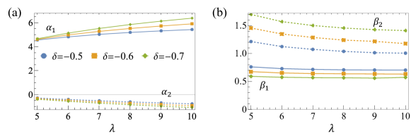
Figure S1: Coefficients of equation of motion (Eq. 1 in main text). $\alpha_{i}$ represent active coefficients and $\beta_{i}$ are passive coefficients.

II.2 Alignment angle

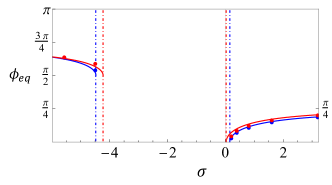
Figure S2: Comparison of alignment angles obtained by integrating the full equation of motion (dots) with those found using analytical approximation (line). Blue: $\lambda=5$, red: $\lambda=10$. Vertical dashed lines separate the regions of alignment. Other parameters: $\delta=-0.6$, $\text{Wi}=0.1$ .

Supplementary Figure S2 shows the comparison of angles of alignment obtained by integrating the analytical equation of motion (Eq. 1 of main text) and those from the eigenvalue analysis. Note that the phase diagram has a weak dependency on aspect ratio.

II.3 Passive spheroid in weakly viscoelastic shear flow

The non-dimensional equation of motion for the orbits is

$$\dot{\bm{p}}=\left(\bm{\mathsf{I}}-\bm{pp}\right)\cdot\left(\bm{\mathsf{E}}^{\infty}\cdot\bm{p}\right)\left[\Lambda+\text{Wi}\,\sigma\alpha_{1}+\text{Wi}\,\beta_{1}\,\bm{\mathsf{E}}^{\infty}:\bm{pp}\right]+\bm{\Omega}^{\infty}\times\bm{p}\left[1+\text{Wi}\,\sigma\alpha_{2}+\text{Wi}\,\beta_{2}\,\bm{\mathsf{E}}^{\infty}:\bm{pp}\right].$$ (S3)

This can be written in the trigonometric form as

$$\dot{\theta}=\frac{\Lambda}{4}\sin 2\theta\sin 2\phi+\text{Wi}\,\beta_{1}\sin^{3}\theta\cos\theta\sin^{2}\phi\cos^{2}\phi$$ (S4a)

$$\dot{\phi}=-\frac{1}{\lambda^{2}+1}\left[\lambda^{2}\sin^{2}\phi+\cos^{2}\phi\right]+\frac{\text{Wi}}{4}\left[\beta_{1}\cos(2\phi)-\beta_{2}\right]\sin^{2}\theta\sin 2\phi.$$ (S4b)

To quantify the log-rolling and compare it with Brunn brunn1977slow , we use the following transformation leal1971effect :

$$\theta=\arctan\left(\frac{C\lambda}{\sqrt{\lambda^{2}\cos^{2}\phi+\sin^{2}\phi}}\right),\quad\tau=\arctan\left(\frac{\tan\phi}{\lambda}\right).$$ (S5)

Here $C$ represents the orbit constant ($C=0$ and $C=\infty$ being the log-rolling and shear-plane rotation orbits, respectively) and $\tau$ is essentially the time coordinate that is scaled with ${T}/{2\pi}$, where $T$ is the Jeffery orbit. Using the above relation, we obtain the evolution equation of the orbit constant as

$$\dot{C}(t) =\text{Wi}\frac{\left[C^{3}\left(\beta_{1}\lambda^{2}-\beta_{2}\lambda^{2}+\beta_{1}+\beta_{2}\right)\sin^{2}\tau\cos^{2}\tau\right]}{2\left(\lambda^{2}C^{2}\cos^{2}\tau+C^{2}\sin^{2}\tau+1\right)},$$

$$\dot{\tau}(t) =\frac{\lambda}{1+\lambda^{2}}+\text{Wi}\left[\frac{\sin\tau\cos\tau\left(2\beta_{1}\lambda^{2}C^{2}\cos^{2}\tau+\beta_{1}+\beta_{2}\right)}{2C^{2}\left(\lambda^{2}\cos^{2}\tau+\sin^{2}\tau\right)+2}-\frac{1}{4}(\beta_{1}+\beta_{2})\sin 2\tau\right].$$ (S6)

We now compare our result with Brunn brunn1977slow who, for a rigid tri-dumbbell, showed that the particle slowly drifts towards the log-rolling orbit. We plot Eq. (II.3) and Eq. (4.17) from Brunn in Supplementary Figure S3 and find a good match. Note that over one period the particle’s orbit declines in a wiggly manner. Interestingly, these wiggles have a physical significance and can be characterized as orbit reduction with two distinct plateaus. Supplementary Figure S3b shows that the long plateau (around $t/T=1/4$) occurs first and is the state where particle is in the vicinity of flow-vorticity plane (where it slows down and spends most of its time). Once the particle exits the alignment state, it flips quickly to the other side ($-x$ axis). This flip generates the short plateau around $t/T=1/2$.

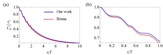
Figure S3: Comparison with Ref. brunn1977slow for the variation of the orbit constant $C/C_{0}$, where $C_{0}$ is the orbit constant for $t=0$. (a) Variation over 10 periods. (b) Variation over one period. Other parameters: $\lambda=5$, $T=2\pi\frac{\lambda^{2}+1}{\lambda}$, $\delta=-0.6$, $\text{Wi}=0.1$.

.

III Details of Kinetic model

Here we provide full expressions and further details involved in the computational steps of kinetic model. The spectral decomposition of $\psi$ is carried out as

$$\psi(\theta,\phi)=\sum_{n=0}^{\infty}\sum_{m=-n}^{n}C_{n,m}(\bm{p})Y_{n}^{m}(\bm{p}).$$ (S7)

Substituting this in the Smoluchowski equation of main text and using the properties of spherical harmonics yields

$$-\frac{1}{4\pi}+\sum_{n=0}^{\infty}\sum_{m=-n}^{n}C_{n,m}\left[1+\tau D_{r}n(n+1)\right]Y_{n}^{m}+\text{Pe}_{f}\sum_{n=0}^{\infty}\sum_{m=-n}^{n}C_{n,m}\mathcal{H}(Y_{n}^{m})=0.$$ (S8)

Here $\mathcal{H}(Y_{n}^{m})$ is a term obtained by simplifying $\nabla_{p}\cdot\left(\dot{\bm{p}}\psi\right)$ and is represented in terms of angular momentum operators for computational convenience chen1996rheology .

$$\mathcal{H}(Y_{n}^{m}) =\left[-\frac{\text{i}\,\mathfrak{L}_{z}}{2}+\frac{\text{i}\Lambda}{2}\left(3\text{i}{Y_{n}^{m}}\sin^{2}(\theta)\sin(2\phi)+\mathfrak{L}_{y}\sin(2\theta)\sin(\phi)+\mathfrak{L}_{z}\cos(2\theta)\sin^{2}(\phi)+\mathfrak{L}_{z}\cos^{2}(\phi)\right)\right]+$$

$$\!\!\!\!\!\!\!\!\!\!\!\!\!\!\text{De}\Bigg{\{}\frac{\text{i}\,\text{Pe}_{a}}{16\pi}\left[\alpha_{1}\left(3\text{i}Y_{n}^{m}\sin^{2}(\theta)\sin(2\phi)+\mathfrak{L}_{y}\sin(2\theta)\sin(\phi)+\mathfrak{L}_{z}\cos(2\theta)\sin^{2}(\phi)+\mathfrak{L}_{z}\cos^{2}(\phi)\right)-\alpha_{2}\mathfrak{L}_{z}\right]+$$

$$\!\!\!\!\!\!\!\frac{\text{i}\,\text{Pe}_{f}}{16}\Big{[}\beta_{1}\sin^{2}(\theta)\Big{(}-iY_{n}^{m}(3+5\cos(2\theta))-10\text{i}Y_{n}^{m}\sin^{2}(\theta)\cos(4\phi)+2\mathfrak{L}_{y}\sin(2\theta)\cos(\phi)-2\mathfrak{L}_{y}\sin(2\theta)\cos(3\phi)+$$

$$\quad 2\mathfrak{L}_{z}\sin^{2}(\theta)\sin(4\phi)+2\mathfrak{L}_{z}\cos(2\theta)\sin(2\phi)+2\mathfrak{L}_{z}\sin(2\phi)\Big{)}+\beta_{2}\sin^{2}(\theta)\left(8\text{i}Y_{n}^{m}\cos(2\phi)-4\mathfrak{L}_{z}\sin(2\phi)\right)\Big{]}\Bigg{\}}.$$ (S9)

Here, the angular momentum operators ($\mathfrak{L}$) are shorthand notation for the following gradients on harmonic $Y_{n}^{m}$:

$$\mathfrak{L}_{y}=L_{y}|Y_{n}^{m}\rangle=-\text{i}\cos\phi\frac{\partial Y_{n}^{m}}{\partial\theta}+\text{i}\cot\theta\sin\phi\frac{\partial Y_{n}^{m}}{\partial\phi}\quad\mbox{and\ }\quad\mathfrak{L}_{z}=L_{z}|Y_{n}^{m}\rangle=-\text{i}\frac{\partial Y_{n}^{m}}{\partial\phi}.$$ (S10)

The trigonometric functions in the Eq. (III) are converted into spherical harmonics. For example:

$$\sin\theta\cos\theta\sin\phi=\text{i}\sqrt{\frac{2\pi}{15}}(Y_{2}^{-1}+Y_{2}^{1}),\quad\cos^{2}\theta=\frac{1}{3}\left(2\sqrt{4\pi/5}Y_{2}^{0}+\sqrt{4\pi}Y_{0}^{0}\right).$$ (S11)

Using such transformations, Eq. (III) yields

$$\mathcal{H}(Y_{n}^{m}) =\Bigg{[}-i\sqrt{\pi}\mathfrak{L}_{z}Y^{0}_{0}+\Lambda\Bigg{(}-\sqrt{\frac{2\pi}{15}}\mathfrak{L}_{y}Y_{2}^{-1}-\sqrt{\frac{2\pi}{15}}\mathfrak{L}_{y}Y_{2}^{1}+i\sqrt{\frac{2\pi}{15}}Y_{2}^{-2}(\mathfrak{L}_{z}-3Y_{n}^{m})+i\sqrt{\frac{2\pi}{15}}Y_{2}^{2}(\mathfrak{L}_{z}+3Y_{n}^{m})$$

$$\qquad\qquad\qquad\qquad\quad+\frac{1}{3}i\sqrt{\pi}\mathfrak{L}_{z}Y_{0}^{0}+\frac{2}{3}i\sqrt{\frac{\pi}{5}}\mathfrak{L}_{z}Y_{2}^{0}\Bigg{)}\Bigg{]}\;+$$

$$\text{De}\Bigg{\{}\text{Pe}_{a}\Bigg{[}-\frac{\text{$\alpha$1}\mathfrak{L}_{y}Y_{2}^{-1}}{4\sqrt{30\pi}}-\frac{\text{$\alpha$1}\mathfrak{L}_{y}Y_{2}^{1}}{4\sqrt{30\pi}}+\frac{i\mathfrak{L}_{z}Y_{0}^{0}(\text{$\alpha$1}-3\text{$\alpha$2})}{24\sqrt{\pi}}+\frac{i\text{$\alpha$1}\mathfrak{L}_{z}Y_{2}^{-2}}{4\sqrt{30\pi}}+\frac{i\text{$\alpha$1}\mathfrak{L}_{z}Y_{2}^{0}}{12\sqrt{5\pi}}+\frac{i\text{$\alpha$1}\mathfrak{L}_{z}Y_{2}^{2}}{4\sqrt{30\pi}}+$$

$$\qquad\qquad-\frac{1}{4}i\sqrt{\frac{3}{10\pi}}\text{$\alpha$1}Y_{n}^{m}Y_{2}^{-2}+\frac{1}{4}i\sqrt{\frac{3}{10\pi}}\text{$\alpha$1}Y_{n}^{m}Y_{2}^{2}\Bigg{]}\;+$$

$$\qquad\;\text{Pe}_{f}\Bigg{[}\frac{1}{7}i\sqrt{\frac{2\pi}{15}}\beta_{1}\mathfrak{L}_{y}Y_{2}^{-1}-\frac{1}{7}i\sqrt{\frac{2\pi}{15}}\beta_{1}\mathfrak{L}_{y}Y_{2}^{1}-\frac{1}{3}i\sqrt{\frac{\pi}{35}}\beta_{1}\mathfrak{L}_{y}Y_{4}^{-3}-\frac{1}{21}i\sqrt{\frac{\pi}{5}}\beta_{1}\mathfrak{L}_{y}Y_{4}^{-1}+\frac{1}{21}i\sqrt{\frac{\pi}{5}}\beta_{1}\mathfrak{L}_{y}Y_{4}^{1}+$$

$$\qquad\qquad\;\frac{1}{3}i\sqrt{\frac{\pi}{35}}\beta_{1}\mathfrak{L}_{y}Y_{4}^{3}-\frac{1}{7}\sqrt{\frac{\pi}{30}}\mathfrak{L}_{z}Y_{2}^{-2}(\beta_{1}-7\beta_{2})+\frac{1}{7}\sqrt{\frac{\pi}{30}}\mathfrak{L}_{z}Y_{2}^{2}(\beta_{1}-7\beta_{2})-\frac{1}{3}\sqrt{\frac{2\pi}{35}}\beta_{1}Y_{4}^{-4}(\mathfrak{L}_{z}-5Y_{n}^{m})+$$

$$\qquad\quad\;\frac{1}{3}\sqrt{\frac{2\pi}{35}}\beta_{1}Y_{4}^{4}(\mathfrak{L}_{z}+5Y_{n}^{m})-\frac{1}{21}\sqrt{\frac{2\pi}{5}}\beta_{1}\mathfrak{L}_{z}Y_{4}^{-2}+\frac{1}{21}\sqrt{\frac{2\pi}{5}}\beta_{1}\mathfrak{L}_{z}Y_{4}^{2}+\frac{2}{7}\sqrt{\frac{\pi}{5}}\beta_{1}Y_{n}^{m}Y_{2}^{0}-\frac{2}{21}\sqrt{\pi}\beta_{1}Y_{n}^{m}Y_{4}^{0}+$$

$$\qquad\quad\;-\sqrt{\frac{2\pi}{15}}\beta_{2}Y_{n}^{m}Y_{2}^{-2}-\sqrt{\frac{2\pi}{15}}\beta_{2}Y_{n}^{m}Y_{2}^{2}\Bigg{]}\Bigg{\}}$$ (S12)

The angular momentum operators are further simplified using the following relations arfken1999mathematical

$$\mathfrak{L}_{y}=L_{y}|Y_{n}^{m}\rangle=\frac{1}{2}\sqrt{n(n+1)-m(m+1)}Y_{n}^{m+1}-\frac{1}{2}\sqrt{n(n+1)-m(m-1)}Y_{n}^{m-1}\quad\mbox{and\ }\quad\mathfrak{L}_{z}=L_{z}|Y_{n}^{m}\rangle=mY_{n}^{m}.$$ (S13)

We substitute above relations in Eq. (III) to simplify $\mathcal{H}(Y_{n}^{m})$ and use that in Eq. (S8). Next, we take an inner product with $\overline{Y_{i}^{j}}$ on both sides of Eq. (S8) and use the orthogonality property to obtain

$$-\frac{1}{4\pi}\int_{S}\overline{Y_{i}^{j}}\text{d}\bm{p}+C_{i,j}\left[1+\tau D_{r}i(i+1)\right]+\text{Pe}_{f}\sum_{n=0}^{\infty}\sum_{m=-n}^{n}C_{n,m}\int_{S}\overline{Y_{i}^{j}}\mathcal{H}(Y_{n}^{m})\text{d}\bm{p}=0.$$ (S14)

The first term is only non-zero for the zeroth mode ($i=0$), which yields $-1/\sqrt{4\pi}$. Since the $C_{0,0}=1/\sqrt{4\pi}$ is already known from normalization, the first term cancels the $i=0$ mode of second term. Using these identities, Eq. (14) can be recasted as the following linear system of equations in terms of $C_{i,j}$:

$$C_{i,j}\left[1+\tau D_{r}i(i+1)\right]+\;\;\text{Pe}_{f}\sum_{n=1}^{100}\sum_{m=-n}^{n}C_{n,m}\int_{S}\overline{Y_{i}^{j}}\mathcal{H}(Y_{n}^{m})\text{d}\bm{p}=-\text{Pe}_{f}C_{0,0}\int_{S}\overline{Y_{i}^{j}}\mathcal{H}(Y_{0}^{0})\text{d}\bm{p},\quad\mbox{ for\ }i\geq 1,$$ (S15)

where the right hand side is known. The two integral terms in the above set of equations contain the inner product of three spherical harmonics. These are represented in terms of Clebsch-Gordon coefficients that exploit the orthogonal relations between harmonics for computational ease arfken1999mathematical :

$$\int_{0}^{\pi}\int_{0}^{2\pi}Y_{N}^{M}Y_{a}^{b}Y_{n}^{m}\,\sin\theta\,\text{d}\phi\text{d}\theta=\sqrt{\frac{(2a+1)(2n+1)}{4\pi(2\text{N}+1)}}\begin{bmatrix}a&n&N\\ 0&0&0\end{bmatrix}\begin{bmatrix}a&n&N\\ b&m&M\end{bmatrix}.$$ (S16)

The bracket terms here are the Clebsch-Gordan coefficients inbuilt in Mathematica 13.

Below we show the match between our results (obtained from the above kinetic model) in the limit $De=0$ and those obtained by Saintillan (saintillan2010dilute, , Fig. 5a, $\tilde{\tau}=1$) .

IV Log-rolling state in the microstructure

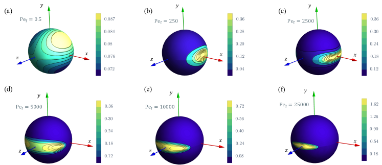
Figure S5: Orientation distribution $\psi(\bm{p})$ of a passive particle with increasing shear rate ($\text{Pe}_{f}$) for $\text{De}=2\times 10^{-5}$, $\lambda=5$, $D_{r}=2\times 10^{-4}\,$s^-1 ($l=30\mu$m).

In Supplementary Figure S5, we illustrate how log-rolling state manifests in the microstructure for large (weakly Brownian) passive particles. We consider a larger particle of length $30\mu$m, which corresponds to $D_{r}=2\times 10^{-4}\,$s^-1. As discussed in the main text, Supplementary Figure S5a shows that when shear is weak, the isotropic distribution of rods is modified primarily by extensional component ($\bm{\mathsf{E}}^{\infty}$) of the shear flow. Hence, the microstructure peaks near the extensional axis. As the shear rate increases, the rotational flow ($\bm{\Omega}^{\infty}$) contributes and the peak shifts towards the flow axis. Supplementary Figure S5b shows that particle almost aligns with the flow direction (positive and negative x-axis). Further increasing $\text{Pe}_{f}$ spreads the distribution in the flow-vorticity plane (Supplementary Figure S5c) and, ultimately for $\text{Pe}_{f}>10^{3}$, a peak develops along the vorticity axis, which is entirely reminiscent of log rolling (Supplementary Figure S5d,e). A further increase concentrates the orientation distribution near the vorticity axis (Supplementary Figure S5f).

References

- (1) Marchetti, M. C. et al. Hydrodynamics of soft active matter. Rev. Mod. Phys. 85, 1143–1189 (2013).
- (2) Zöttl, A. & Stark, H. Emergent behavior in active colloids. J. Phys. Condens. Matter 28, 253001 (2016).
- (3) Lauga, E. The fluid dynamics of cell motility, vol. 62 (Cambridge University Press, 2020).
- (4) Berg, H. C. & Brown, D. A. Chemotaxis in escherichia coli analysed by three-dimensional tracking. Nature 239, 500–504 (1972).
- (5) Demir, M. & Salman, H. Bacterial thermotaxis by speed modulation. Biophys. J. 103, 1683–1690 (2012).
- (6) Stark, H. Artificial chemotaxis of self-phoretic active colloids: Collective behavior. Acc. Chem. Res. 51, 2681–2688 (2018).
- (7) Mathijssen, A. J. et al. Oscillatory surface rheotaxis of swimming e. coli bacteria. Nat. Comm. 10, 1–12 (2019).
- (8) Jing, G., Zöttl, A., Clément, É. & Lindner, A. Chirality-induced bacterial rheotaxis in bulk shear flows. Sci. Adv. 6, eabb2012 (2020).
- (9) Doan, V. S., Saingam, P., Yan, T. & Shin, S. A trace amount of surfactants enables diffusiophoretic swimming of bacteria. ACS nano 14, 14219–14227 (2020).
- (10) Ramamonjy, A., Dervaux, J. & Brunet, P. Nonlinear phototaxis and instabilities in suspensions of light-seeking algae. Phys. Rev. Lett. 128, 258101 (2022).
- (11) Suarez, S. S. & Pacey, A. Sperm transport in the female reproductive tract. Hum. Reprod. Update 12, 23–37 (2006).
- (12) Zöttl, A. & Stark, H. Nonlinear dynamics of a microswimmer in poiseuille flow. Phys. Rev. Lett. 108, 218104 (2012).
- (13) Sznitman, J. & Arratia, P. E. Locomotion through complex fluids: an experimental view (Springer, 2015).
- (14) Shogren, R., Gerken, T. A. & Jentoft, N. Role of glycosylation on the conformation and chain dimensions of o-linked glycoproteins: light-scattering studies of ovine submaxillary mucin. Biochem. 28, 5525–5536 (1989).
- (15) Lai, S. K., Wang, Y.-Y., Wirtz, D. & Hanes, J. Micro-and macrorheology of mucus. Adv. Drug Deliv. Rev. 61, 86–100 (2009).
- (16) Mathijssen, A. J., Shendruk, T. N., Yeomans, J. M. & Doostmohammadi, A. Upstream swimming in microbiological flows. Phys. Rev. Lett. 116, 028104 (2016).
- (17) Choudhary, A. & Stark, H. On the cross-streamline lift of microswimmers in viscoelastic flows. Soft Matter 18, 48–52 (2022).
- (18) Sokolov, A. & Aranson, I. S. Reduction of viscosity in suspension of swimming bacteria. Phys. Rev. Lett. 103, 148101 (2009).
- (19) Gachelin, J. et al. Non-newtonian viscosity of escherichia coli suspensions. Phys. Rev. Lett. 110, 268103 (2013).
- (20) McDonnell, A. G. et al. Motility induced changes in viscosity of suspensions of swimming microbes in extensional flows. Soft Matter 11, 4658–4668 (2015).
- (21) López, H. M., Gachelin, J., Douarche, C., Auradou, H. & Clément, E. Turning bacteria suspensions into superfluids. Phys. Rev. Lett. 115, 028301 (2015).
- (22) Hatwalne, Y., Ramaswamy, S., Rao, M. & Simha, R. A. Rheology of active-particle suspensions. Phys. Rev. Lett. 92, 118101 (2004).
- (23) Haines, B. M., Sokolov, A., Aranson, I. S., Berlyand, L. & Karpeev, D. A. Three-dimensional model for the effective viscosity of bacterial suspensions. Phys. Rev. E 80, 041922 (2009).
- (24) Saintillan, D. The dilute rheology of swimming suspensions: A simple kinetic model. Exp. Mech. 50, 1275–1281 (2010).
- (25) Jeffery, G. B. The motion of ellipsoidal particles immersed in a viscous fluid. Proc. R. Soc. Lond.. 102, 161–179 (1922).
- (26) Rafaï, S., Jibuti, L. & Peyla, P. Effective viscosity of microswimmer suspensions. Phys. Rev. Lett. 104, 098102 (2010).
- (27) Li, G. & Ardekani, A. M. Collective motion of microorganisms in a viscoelastic fluid. Phys. Rev. Lett. 117, 118001 (2016).
- (28) Li, G., Lauga, E. & Ardekani, A. M. Microswimming in viscoelastic fluids. J. Non-Newton. Fluid Mech. 297, 104655 (2021).
- (29) Spagnolie, S. E. & Underhill, P. T. Swimming in complex fluids. Annu. Rev. Condens. 14, 381–415 (2023).
- (30) Patteson, A., Gopinath, A., Goulian, M. & Arratia, P. Running and tumbling with e. coli in polymeric solutions. Sci. Rep. 5, 15761 (2015).
- (31) Zöttl, A. & Yeomans, J. M. Enhanced bacterial swimming speeds in macromolecular polymer solutions. Nat. Phys. 15, 554–558 (2019).
- (32) Kamdar, S. et al. The colloidal nature of complex fluids enhances bacterial motility. Nature 603, 819–823 (2022).
- (33) Liu, S., Shankar, S., Marchetti, M. C. & Wu, Y. Viscoelastic control of spatiotemporal order in bacterial active matter. Nature 590, 80–84 (2021).
- (34) De Corato, M. & D’Avino, G. Dynamics of a microorganism in a sheared viscoelastic liquid. Soft Matter 13, 196–211 (2017).
- (35) Bird, R. B., Curtiss, C. F., Armstrong, R. C. & Hassager, O. Dynamics of polymeric liquids, volume 1: fluid mechanics (Wiley, 1987).
- (36) James, D. F. Boger fluids. Annu. Rev. Fluid Mech. 41, 129–142 (2009).
- (37) Leal, L. The slow motion of slender rod-like particles in a second-order fluid. J. Fluid. Mech. 69, 305–337 (1975).
- (38) Brunn, P. The slow motion of a rigid particle in a second-order fluid. J. Fluid Mech. 82, 529–547 (1977).
- (39) Hinch, E. & Leal, L. Constitutive equations in suspension mechanics. part 1. general formulation. J. Fluid. Mech. 71, 481–495 (1975).
- (40) Chwang, A. T. & Wu, T. Y.-T. Hydromechanics of low-reynolds-number flow. part 2. singularity method for stokes flows. J. Fluid. Mech. 67, 787–815 (1975).
- (41) Spagnolie, S. E. & Lauga, E. Hydrodynamics of self-propulsion near a boundary: predictions and accuracy of far-field approximations. J. Fluid Mech. 700, 105–147 (2012).
- (42) Berke, A. P., Turner, L., Berg, H. C. & Lauga, E. Hydrodynamic attraction of swimming microorganisms by surfaces. Phys. Rev. Lett. 101, 038102 (2008).
- (43) Drescher, K., Goldstein, R. E., Michel, N., Polin, M. & Tuval, I. Direct measurement of the flow field around swimming microorganisms. Phys. Rev. Lett. 105, 168101 (2010).
- (44) Ebagninin, K. W., Benchabane, A. & Bekkour, K. Rheological characterization of poly (ethylene oxide) solutions of different molecular weights. J. Colloid Interface Sci. 336, 360–367 (2009).
- (45) Einarsson, J., Candelier, F., Lundell, F., Angilella, J. & Mehlig, B. Rotation of a spheroid in a simple shear at small reynolds number. Phys. Fluids 27, 063301 (2015).
- (46) Gauthier, F., Goldsmith, H. & Mason, S. Particle motions in non-newtonian media. Rheol. Acta 10, 344–364 (1971).
- (47) D’Avino, G. & Maffettone, P. L. Particle dynamics in viscoelastic liquids. J. Non-Newton. Fluid Mech. 215, 80–104 (2015).
- (48) Berg, H. Random Walks in Biology. Princeton Univ. Press, Princeton, NJ (1983).
- (49) Lauga, E. Bacterial hydrodynamics. Ann. Rev. Fluid Mech. 48, 105–130 (2016).
- (50) Adhyapak, T. C. & Stark, H. Dynamics of a bacterial flagellum under reverse rotation. Soft Matter 12, 5621–5629 (2016).
- (51) Nambiar, S., Nott, P. & Subramanian, G. Stress relaxation in a dilute bacterial suspension. J. Fluid. Mech. 812, 41–64 (2017).
- (52) Doi, M., Edwards, S. F. & Edwards, S. F. The theory of polymer dynamics, vol. 73 (Oxford University Press, 1988).
- (53) Cohen, C., Chung, B. & Stasiak, W. Orientation and rheology of rodlike particles with weak brownian diffusion in a second-order fluid under simple shear flow. Rheo. Acta 26, 217–232 (1987).
- (54) Chattopadhyay, S., Moldovan, R., Yeung, C. & Wu, X. Swimming efficiency of bacterium escherichiacoli. Proc. Natl. Acad. Sci. U.S.A. 103, 13712–13717 (2006).
- (55) Hinch, E. & Leal, L. Constitutive equations in suspension mechanics. part 2. approximate forms for a suspension of rigid particles affected by brownian rotations. J. Fluid. Mech. 76, 187–208 (1976).
- (56) Chen, S. B. & Koch, D. L. Rheology of dilute suspensions of charged fibers. Phys. Fluids 8, 2792–2807 (1996).
- (57) Hinch, E. & Leal, L. The effect of brownian motion on the rheological properties of a suspension of non-spherical particles. J. Fluid. Mech. 52, 683–712 (1972).
- (58) Wolfe, A. J., Conley, M. P. & Berg, H. C. Acetyladenylate plays a role in controlling the direction of flagellar rotation. Proc. Natl. Acad. Sci. U.S.A. 85, 6711–6715 (1988).
- (59) Chung, B. & Cohen, C. Orientation and rheology of rodlike particles with strong brownian diffusion in a second-order fluid under simple shear flow. J. Nonnewton. Fluid Mech. 25, 289–312 (1987).
- (60) Leal, L. & Hinch, E. The effect of weak brownian rotations on particles in shear flow. J. Fluid. Mech. 46, 685–703 (1971).
- (61) Elgeti, J., Winkler, R. G. & Gompper, G. Physics of microswimmers—single particle motion and collective behavior: a review. Rep. Prog. Phys. 78, 056601 (2015).
- (62) Junot, G. et al. Swimming bacteria in poiseuille flow: The quest for active bretherton-jeffery trajectories. Europhys. Lett. 126, 44003 (2019).
- (63) Brown, A., Clarke, S., Convert, P. & Rennie, A. Orientational order in concentrated dispersions of plate-like kaolinite particles under shear. J. Rheol. 44, 221–233 (2000).
- (64) Batchelor, G. The stress system in a suspension of force-free particles. J. Fluid. Mech. 41, 545–570 (1970).
- (65) Einstein, A. A new determination of molecular dimensions. Ann. Phys. 19, 289–306 (1906).
- (66) Férec, J., Bertevas, E., Khoo, B., Ausias, G. & Phan-Thien, N. Steady-shear rheological properties for suspensions of axisymmetric particles in second-order fluids. J. Non-Newton. Fluid Mech. 239, 62–72 (2017).
- (67) Bird, R. B., Curtiss, C. F., Armstrong, R. C. & Hassager, O. Dynamics of polymeric liquids, volume 2: Kinetic theory (Wiley, 1987).
- (68) Ren, L. et al. 3d steerable, acoustically powered microswimmers for single-particle manipulation. Sci. Adv. 5, 3084 (2019).
- (69) Aghakhani, A., Yasa, O., Wrede, P. & Sitti, M. Acoustically powered surface-slipping mobile microrobots. Proc. Natl. Acad. Sci. U.S.A. 117, 3469–3477 (2020).
- (70) Guo, S., Samanta, D., Peng, Y., Xu, X. & Cheng, X. Symmetric shear banding and swarming vortices in bacterial superfluids. Proc. Natl. Acad. Sci. U.S.A. 115, 7212–7217 (2018).
- (71) Aranson, I. Bacterial active matter. Rep. Prog. Phys. (2022).
- (72) Bozorgi, Y. & Underhill, P. T. Effect of viscoelasticity on the collective behavior of swimming microorganisms. Phys. Rev. E 84, 061901 (2011).
- (73) Ardekani, A. M. & Gore, E. Emergence of a limit cycle for swimming microorganisms in a vortical flow of a viscoelastic fluid. Phys. Rev. E 85, 056309 (2012).
- (74) Narinder, N., Bechinger, C. & Gomez-Solano, J. R. Memory-induced transition from a persistent random walk to circular motion for achiral microswimmers. Phys. Rev. Lett. 121, 078003 (2018).
- (75) Abtahi, S. A. & Elfring, G. J. Jeffery orbits in shear-thinning fluids. Phys. Fluids 31, 103106 (2019).
- (76) Elfring, G. J. & Lauga, E. Theory of locomotion through complex fluids. In Complex fluids in biological systems, 283–317 (Springer, 2015).
- (77) Bretherton, F. P. The motion of rigid particles in a shear flow at low reynolds number. J. Fluid Mech. 14, 284–304 (1962).
- (78) Einarsson, J. Angular dynamics of small particles in fluids (2015).
- (79) Strogatz, S. H. Nonlinear dynamics and chaos: with applications to physics, biology, chemistry, and engineering (CRC Press, 2018).
- (80) Arfken, G. B. & Weber, H. J. Mathematical methods for physicists (Academic Press Orlando, FL, 1972).