Cascaded variational quantum eigensolver algorithm

Abstract

We present a cascaded variational quantum eigensolver algorithm that only requires the execution of a set of quantum circuits once rather than at every iteration during the parameter optimization process, thereby reducing the number of needed circuit executions. This algorithm uses a quantum processing unit to probe the needed probability mass functions and a classical processing unit perform the remaining calculations, including the energy minimization. The ansatz form does not restrict the Fock space and provides full control over the ansatz state, including the implementation of symmetry and other physically motivated constraints.

Quantum computing (QC) offers inherent advantages over classical computing (CC) for solving certain mathematical tasks [1, 2, 3, 4, 5, 6, 7, 8]. One of the most promising application areas is the simulation of quantum-mechanical systems [7, 9, 10]. Because the dimension of the Hilbert space that comprises the quantum states of a fermionic system increases exponentially with the system size, performing operations on this space is an intractable task for conventional classical computers, for all but the smallest systems. A quantum computer, on the other hand, can process such a Hilbert space by mapping it to the Hilbert space of a quantum register—the size of which increases exponentially with the number of qubits—and then performing quantum gate operations on this register.

The two main algorithms for QC calculations of quantum-mechanical systems are the quantum phase estimation algorithm [11] and the variational quantum eigensolver (VQE) algorithm [12]. By recruiting classical computers for computationally efficient tasks, the latter algorithm requires relatively few gate operations, which limits the decoherence during the computations. As less exposure to decoherence allows for higher computational fidelities, this algorithm has a reduced need for quantum error correction, making it ideal for current noisy intermediate-scale quantum (NISQ) computers [13]. Since its introduction, the VQE algorithm has been applied to calculate the ground-state energy of a number of systems in chemistry and physics [12, 14, 15, 16, 17, 18, 19, 20, 21, 22, 23, 24, 25, 26, 27, 28, 29, 30, 31, 32, 33].

One downside of the VQE algorithm caused by the quantum circuits being dependent on the variational parameters is that the algorithm necessarily involves a lot of back-and-forth communication between the quantum processing unit (QPU) and the classical processing unit (CPU) during the energy minimization process. This process, furthermore, increases the already relatively large number of required quantum circuit executions, thereby reducing computational throughput.

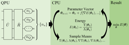
Figure 1: Schematic of the cascaded variational quantum eigensolver algorithm. The QPU executes a set of quantum circuits, each generating a unique quantum state $\hat{R}\hat{U}\!\ket{0}$ that when measured yield a family of occupation numbers $(n_{1},n_{2},...,n_{Q})$ recorded as $n_{s}$. Repeating the same measurements multiple times produces sets of families $\{n_{s}\}$ that are passed on as input to the CPU. The CPU uses these samples together with a parameter vector $\boldsymbol{\theta}_{k}$ to compute derivatives of the energy $E(\boldsymbol{\theta})$ of the ansatz state $\ket{\Psi(\boldsymbol{\theta})}$ at $\boldsymbol{\theta}=\boldsymbol{\theta}_{k}$ by obtaining sample means for $\Upsilon(\boldsymbol{\theta}_{k})$, $\Lambda(\boldsymbol{\theta}_{k})$, $\nabla\Upsilon(\boldsymbol{\theta}_{k})$, and $\nabla\Lambda(\boldsymbol{\theta}_{k})$ from Eq. (12), (19), and (22). These derivatives are then used to generate a new parameter vector $\boldsymbol{\theta}_{k+1}$, using some optimization method $f[\nabla E(\boldsymbol{\theta}_{k}),...]$, and the process is repeated until the optimization has been completed and the sought minimum energy obtained.

To address these challenges, we propose the cascaded variational quantum eigensolver (CVQE) algorithm, in which the variational parameters are exclusively processed on the CPU. This is possible as the number of variational parameters only increases polynomially with the system size. However, the QPU is still needed to sample the possible outcomes of an initial state measured in various bases, a task that cannot in general be performed efficiently on a CPU, as the probability distributions are generally unknown and the number of possible outcomes increases exponentially with the system size. As illustrated in Fig. 1, given the samples from an initial set of measurements, the energy minimization can subsequently be completed on the CPU alone, without further involvement of the QPU. This approach thus both eliminates the back-and-forth communication between the QPU and CPU and reduces the number of needed quantum circuit executions, typically by two to three orders of magnitude.

In order to demonstrate the method behind the CVQE algorithm, consider a system of identical fermions described by the Hamiltonian $\hat{H}$ and let the antisymmetric Fock space $\mathcal{F}$ serve as the representation space for the quantum states of this system. Our goal is to get an upper bound for the ground-state energy $E_{\text{g}}$ of the system by applying the variational method of quantum mechanics, which can be stated as

$$E_{\text{g}}\leq\min_{\boldsymbol{\theta}}E(\boldsymbol{\theta}),$$ (1)

where $\boldsymbol{\theta}$ is a variational parameter vector in the parameter space $\Theta$, which is a subset of the $d$-dimensional real coordinate space $\mathbb{R}^{d}$, and $E(\boldsymbol{\theta})$ is the energy of the state $\ket{\Psi(\boldsymbol{\theta})}$ in the ansatz.

We construct the ansatz state $\ket{\Psi(\boldsymbol{\theta})}$ from the normalized state

$$\ket{\Psi_{0}}=\hat{U}\ket{0},$$ (2)

where $\hat{U}$ is a unitary operator and $\ket{0}$ is the vacuum state in $\mathcal{F}$, that we represent on the QPU for sampling. In contrast to the unitary operators applied on the QPU in the commonly used unitary coupled cluster ansatz [34, 12, 14, 15, 35, 36, 37, 38, 39, 40, 41, 42, 43, 44, 45, 46, 47, 48], the hardware-efficient ansatz [18, 49, 50, 51, 52, 53, 54, 55, 56], and those used in various adaptive or trainable VQE algorithms [57, 58, 59, 60, 61, 62, 63, 64, 65], we require that $\hat{U}$ be independent of $\boldsymbol{\theta}$. Instead, we introduce the dependence on $\boldsymbol{\theta}$ through the operator $e^{i\hat{\lambda}(\boldsymbol{\theta})}$ that transforms $\ket{\Psi_{0}}$ to our ansatz state

$$\ket{\Psi(\boldsymbol{\theta})}=e^{i\hat{\lambda}(\boldsymbol{\theta})}\ket{\Psi_{0}},$$ (3)

where $\hat{\lambda}(\boldsymbol{\theta})$ is an operator. Consequently, the energy of $\ket{\Psi(\boldsymbol{\theta})}$ is of the form

$$E(\boldsymbol{\theta})=\frac{\Upsilon(\boldsymbol{\theta})}{\Lambda(\boldsymbol{\theta})},$$ (4)

with the expectation values

$$\Upsilon(\boldsymbol{\theta})= \braket{\Psi_{0}}{e^{-i\hat{\lambda}^{\dagger}(\boldsymbol{\theta})}\hat{H}e^{i\hat{\lambda}(\boldsymbol{\theta})}}{\Psi_{0}},$$ (5a)

$$\Lambda(\boldsymbol{\theta})= \braket{\Psi_{0}}{e^{-i\hat{\lambda}^{\dagger}(\boldsymbol{\theta})}e^{i\hat{\lambda}(\boldsymbol{\theta})}}{\Psi_{0}}.$$ (5b)

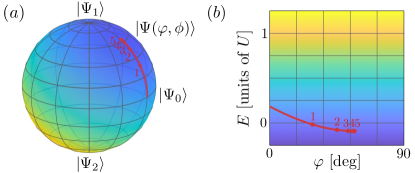
Figure 2: The energy $E(\varphi,\phi)$ of the singlet two-fermion ansatz state $\ket{\Psi(\varphi,\phi)}$ of the two-site Hubbard model with the Hamiltonian $\hat{H}=t\sum_{\sigma}\big{(}c_{0\sigma}^{\dagger}c_{1\sigma}^{\mathstrut}+\text{h.c.}\big{)}+U\sum_{i}c_{i\uparrow}^{\dagger}c_{i\downarrow}^{\dagger}c_{i\downarrow}^{\mathstrut}c_{i\uparrow}^{\mathstrut}$, where $t$ and $U$ are coefficients and $i\in\{0,1\}$ and $\sigma\in\{\uparrow,\downarrow\}$ are site and spin indices, respectively, so that all index pairs are elements in the one-fermion index set $({0\!\uparrow},{0\!\downarrow},{1\!\uparrow},{1\!\downarrow})$. The parameter space has been restricted by letting $\lambda_{n}\!\rightarrow i\infty$ for all families $n$ of occupation numbers, except for those associated with two fermions with a zero $z$ component of the total spin. Permutation symmetry requires that singlet states transform as $A_{1g}$ in the point group $D_{\infty h}$, which means that $\ket{\Psi(\varphi,\phi)}$ is a linear combination of $\ket{\Psi_{1}}=\big{(}\!\ket{0110}+\ket{1001}\!\big{)}/\sqrt{2}$ and $\ket{\Psi_{2}}=\big{(}\!\ket{0011}+\ket{1100}\!\big{)}/\sqrt{2}$. This requirement is imposed by the symmetry constraints $\lambda_{0110}\!=\!\lambda_{1001}\!=\!\lambda$ and $\lambda_{0011}\!=\!\lambda_{1100}\!=\!-\lambda$. The parametric equation $\lambda=\lambda(\varphi,\phi)=\phi/2-i\ln\tan\big{(}\frac{\pi}{4}\!+\!\frac{\varphi}{2}\big{)}/2$ is defined on the parameter space $\{(\varphi,\phi)\!:\!\varphi\!\in\!(-\pi/2,\pi/2),\phi\!\in\!(-\pi,\pi]\}$, where $\varphi$ and $\phi$ represent the latitude and longitude, respectively, on a sphere. The energy $E(\varphi,\phi)$ for $t/U=-0.158$ is shown in color in (a) with the colorbar in (b). The red curves trace the gradient-descent path along $\phi=0$ from the initial QPU state $\ket{\Psi_{0}}=\big{(}\!\ket{\Psi_{1}}+\ket{\Psi_{2}}\!\big{)}/\sqrt{2}$ to the ground state at $\varphi\approx 1$ rad.

To make further progress, we need a basis for the Fock space $\mathcal{F}$. First, however, we introduce the totally ordered index set $\mathcal{Q}$ for the basis $(\ket{\psi_{q}})_{q\in\mathcal{Q}}$ for the one-fermion Hilbert space $\mathcal{H}$. The cardinality $Q$ of this set (i.e., the dimension of $\mathcal{H}$) is herein our measure of the system size. Each $q\in\mathcal{Q}$ has an occupation number $n_{q}$ in $\{0,1\}$ that is zero if $\ket{\psi_{q}}$ is unoccupied and one if it is occupied. Each family of occupation numbers $n=(n_{q})_{q\in\mathcal{Q}}$ in the Cartesian power $\mathcal{N}=\{0,1\}^{Q}$ identifies the associated operator

$$C_{n}^{\dagger}=\prod_{q\in\mathcal{Q}}\big{(}c^{\dagger}_{q}\big{)}^{n_{q}},$$ (6)

on $\mathcal{F}$, where $c_{q}^{\dagger}$ is the fermionic creation operator associated with $q$ in $\mathcal{Q}$. Using these operators, we generate the Fock states $\ket{n}=C_{n}^{\dagger}\ket{0}$, for all $n\in\mathcal{N}$, and then select the set of all Fock states $\{\ket{n}:n\in\mathcal{N}\}$ to be our basis for $\mathcal{F}$.

We choose the operator $\hat{\lambda}(\boldsymbol{\theta})$ be diagonal in this basis, so that

$$\hat{\lambda}(\boldsymbol{\theta})=\sum_{n\in\mathcal{N}}\lambda_{n}(\boldsymbol{\theta})\ket{n}\!\bra{n},$$ (7)

where $\lambda_{n}(\boldsymbol{\theta})\in\mathbb{C}$ is a complex parametric equation. Our ansatz state in Eq. (3) can thus be expressed as

$$\ket{\Psi(\boldsymbol{\theta})}=\sum_{n\in\mathcal{N}}e^{i\lambda_{n}(\boldsymbol{\theta})}\Psi_{0n}\ket{n},$$ (8)

where $\Psi_{0n}$ is the component of $\ket{\Psi_{0}}$ associated with $\ket{n}$. This form is both general and intuitive. It is general because if we choose our set $\{\lambda_{n}(\boldsymbol{\theta}):n\in\mathcal{N}\}$ of parametric equations to be a surjective map of $\Theta$ onto $\mathbb{C}^{2^{Q}}$ and our components $\Psi_{0n}$ to be nonzero, for all $n\in\mathcal{N}$, then the ansatz covers the entire Fock space. It is intuitive because each $\lambda_{n}(\boldsymbol{\theta})$ is associated with a Fock state $\ket{n}$, which allows us to both exclude specific Fock states by letting $\lambda_{n}(\boldsymbol{\theta})\!\rightarrow i\infty$ and impose symmetry constraints provided in terms of Fock states on our set $\{\lambda_{n}(\boldsymbol{\theta}):n\in\mathcal{N}\}$. An example of a set of parametric equations that both exclude states and impose symmetry constraints is provided in the caption of Fig. 2 and in the Supplemental Material (SM), for a singlet two-fermion ansatz state of the two-site Hubbard model. We can even choose our ansatz to depend on number operators as in the recent implementation [66] of the Jastrow–Gutzwiller ansatz [67, 68] within the CVQE algorithm, where $\lambda_{n}(\boldsymbol{\theta})=\sum_{qq^{\prime}\in\mathcal{Q}}i\theta_{qq^{\prime}}n_{q}n_{q^{\prime}}$.

As the dimension of $\mathcal{F}$ is $2^{Q}$, and thus increases exponentially with the system size $Q$, the energy in Eq. (4) cannot in general be calculated efficiently using a CPU alone, which is why we need the assistance of a QPU. Because qubits are distinguishable, the Hilbert space for a qubit register in the QPU is a tensor power of the two-dimensional one-qubit Hilbert space $\mathtt{H}$. For there to be an isomorphism between the Fock space and this tensor power, we need a register that comprises exactly $Q$ qubits, so that $\dim\mathtt{H}^{\otimes Q}$ equals $\dim\mathcal{F}$. We select $\{\ket{0},\ket{1}\}$ to be our basis for each qubit space $\mathtt{H}$ and define the isomorphism $\mathcal{F}\rightarrow\mathtt{H}^{\otimes Q}$ by mapping the Fock states $\ket{n}$ to the tensor products

$$\ket{n}=\bigotimes_{q\in\mathcal{Q}}\ket{n_{q}},$$ (9)

for all $n\in\mathcal{N}$. This Jordan–Wigner mapping maps $\ket{\Psi_{0}}$ to $\ket{\Psi_{0}}$ and thus preserves all its components $\Psi_{0n}$. This makes it straightforward to construct a quantum circuit for $\hat{U}$ that uses –$X$– gates to generate the ground state $\ket{n^{*}}$ of some model of the system within the independent fermion approximation, for which the components are $\Psi_{0n}=\delta_{nn^{*}}$, where $\delta$ is the Kronecker delta, and from there introduce weights associated with other Fock states by adding additional gates.

In our sampling on the QPU, we use the fact that the probability that a measurement in the basis $\{\ket{n}:n\in\mathcal{N}\}$ would collapse the state $\hat{R}\ket{\Psi_{0}}$, for any unitary operator $\hat{R}$, to the state $\ket{n}$ associated with a particular outcome $n$ in the sample space $\mathcal{N}$ is given by the probability mass function

$$\operatorname{P}[\hat{R}\Psi_{0}\!\mapsto\!n]=\big{|}\!\braket{\Psi_{0}}{\hat{R}^{\dagger}}{n}\!\big{|}^{2}.$$ (10)

By performing $S$ identical measurements of $\hat{R}\ket{\Psi_{0}}$ and recording the outcome $n_{s}$ of each shot $s$ in some set $\mathcal{S}$, we obtain a set of families $\{n_{s}:s\in\mathcal{S}\}$. Given this sample, we can then apply the law of the unconscious statistician and approximate the expectation value of a function $g(n)$ with the arithmetic mean, which yields

$$\sum_{n\in\mathcal{N}}g(n)\operatorname{P}[\hat{R}\Psi_{0}\!\mapsto\!n]\approx\frac{1}{S}\sum_{s\in\mathcal{S}}g(n_{s}),$$ (11)

where the sample size $S$ is chosen such that the desired statistical accuracy is attained.

The challenge with calculating expectation values with the assistance of a QPU is that the operators must be diagonal in the measurement basis. One operator that is already diagonal is $e^{-i\hat{\lambda}^{\dagger}(\boldsymbol{\theta})}e^{i\hat{\lambda}(\boldsymbol{\theta})}$. We thus perform a set of measurements of $\ket{\Psi_{0}}$ to obtain the sample $\{n_{s}^{0}:s\in\mathcal{S}\}$ and then use this sample to calculate the sample mean of the expectation value in Eq. (5b)

$$\Lambda(\boldsymbol{\theta})\approx\frac{1}{S}\sum_{s\in\mathcal{S}}e^{-2\operatorname{Im}\lambda_{n_{s}^{0}}(\boldsymbol{\theta})}$$ (12)

on a CPU.

Because the dimension of $\mathcal{F}$ increases exponentially with the system size, we cannot generally diagonalize $e^{-i\hat{\lambda}^{\dagger}(\boldsymbol{\theta})}\hat{H}e^{i\hat{\lambda}(\boldsymbol{\theta})}$ on a CPU for large $Q$. Instead, we note that the expectation value of an operator is a linear function, which allows us to expand the expectation value in Eq. (5a) and diagonalize the operator in each expectation value independently.

Table 1: The coefficients $h_{l}$, operators $C_{n_{l}^{+}}^{\dagger}C_{n_{l}^{-}\vphantom{{}^{+}}}\vphantom{{}^{\dagger}}$, families $n_{l}^{\pm}$, subsets $\dot{\mathcal{Q}}_{l}$ and $\vec{\mathcal{Q}}_{l}$, and subfamilies $\dot{n}_{l}^{\pm}$ and $\vec{n}_{l}^{\pm}$ for each interaction in the two-site Hubbard model with the Hamiltonian $\hat{H}=t\sum_{\sigma}\big{(}c_{0\sigma}^{\dagger}c_{1\sigma}^{\mathstrut}+\text{h.c.}\big{)}+U\sum_{i}c_{i\uparrow}^{\dagger}c_{i\downarrow}^{\dagger}c_{i\downarrow}^{\mathstrut}c_{i\uparrow}^{\mathstrut}$, where $t$ and $U$ are coefficients and $i\in\{0,1\}$ and $\sigma\in\{\uparrow,\downarrow\}$ are site and spin indices, respectively, so that all index pairs are elements in $\mathcal{Q}=({0\!\uparrow},{0\!\downarrow},{1\!\uparrow},{1\!\downarrow})$.

$\quad~{}~{}h_{l}\quad~{}~{}$	$\quad C_{n_{l}^{+}}^{\dagger}C_{n_{l}^{-}\vphantom{{}^{+}}}\vphantom{{}^{\dagger}}\quad$	$\qquad n_{l}^{+}\qquad$	$\qquad n_{l}^{-}\qquad$	$\qquad\dot{\mathcal{Q}}_{l}\qquad$	$\qquad\vec{\mathcal{Q}}_{l}\qquad$	$\quad~{}{\dot{n}}_{l}^{+}\quad~{}$	$\qquad\vec{n}_{l}^{+}\qquad$	$\quad~{}{\dot{n}}_{l}^{-}\quad~{}$	$\qquad\vec{n}_{l}^{-}\qquad$
$t$	$c_{0\uparrow}^{\dagger}c_{1\uparrow}^{\mathstrut}$	$(1,0,0,0)$	$(0,0,1,0)$	$(0\!\uparrow,1\!\uparrow)$	$(0\!\downarrow,1\!\downarrow)$	$(1,0)$	$(0,0)$	$(0,1)$	$(0,0)$
$t$	$c_{1\uparrow}^{\dagger}c_{0\uparrow}^{\mathstrut}$	$(0,0,1,0)$	$(1,0,0,0)$	$(0\!\uparrow,1\!\uparrow)$	$(0\!\downarrow,1\!\downarrow)$	$(0,1)$	$(0,0)$	$(1,0)$	$(0,0)$
$t$	$c_{0\downarrow}^{\dagger}c_{1\downarrow}^{\mathstrut}$	$(0,1,0,0)$	$(0,0,0,1)$	$(0\!\downarrow,1\!\downarrow)$	$(0\!\uparrow,1\!\uparrow)$	$(1,0)$	$(0,0)$	$(0,1)$	$(0,0)$
$t$	$c_{1\downarrow}^{\dagger}c_{0\downarrow}^{\mathstrut}$	$(0,0,0,1)$	$(0,1,0,0)$	$(0\!\downarrow,1\!\downarrow)$	$(0\!\uparrow,1\!\uparrow)$	$(0,1)$	$(0,0)$	$(1,0)$	$(0,0)$
$U$	$c_{0\uparrow}^{\dagger}c_{0\downarrow}^{\dagger}c_{0\downarrow}^{\mathstrut}c_{0\uparrow}^{\mathstrut}$	$(1,1,0,0)$	$(1,1,0,0)$	$(~{})$	$(0\!\uparrow,0\!\downarrow,1\!\uparrow,1\!\downarrow)$	$(~{})$	$(1,1,0,0)$	$(~{})$	$(1,1,0,0)$
$U$	$c_{1\uparrow}^{\dagger}c_{1\downarrow}^{\dagger}c_{1\downarrow}^{\mathstrut}c_{1\uparrow}^{\mathstrut}$	$(0,0,1,1)$	$(0,0,1,1)$	$(~{})$	$(0\!\uparrow,0\!\downarrow,1\!\uparrow,1\!\downarrow)$	$(~{})$	$(0,0,1,1)$	$(~{})$	$(0,0,1,1)$

We express the Hamiltonian, using the operators in Eq. (6), in the form of

$$\hat{H}=\sum_{l\in\mathcal{L}}h_{l}\,C_{n_{l}^{+}}^{\dagger}C_{n_{l}^{-}\vphantom{{}^{+}}}\vphantom{{}^{\dagger}},$$ (13)

where the set $\mathcal{L}$ contains all nonzero interactions $l$, each specified by a coefficient $h_{l}\in\mathbb{C}$ and two families $n_{l}^{\pm}=(n_{lq}^{\pm})_{q\in\mathcal{Q}}$ in $\mathcal{N}$, in which the bits are defined by

$$n_{lq}^{+}=\left\{\begin{aligned} 1,&\qquad\text{if }c_{q}^{\dagger}\text{ is \phantom{\text@underline{not}} present},\\ 0,&\qquad\text{if }c_{q}^{\dagger}\text{ is \text@underline{not} present},\end{aligned}\right.$$ (14a)

$$n_{lq}^{-}=\left\{\begin{aligned} 1,&\qquad\text{if }c_{q}\text{ is \phantom{\text@underline{not}} present},\\ 0,&\qquad\text{if }c_{q}\text{ is \text@underline{not} present},\end{aligned}\right.$$ (14b)

in the interaction Hamiltonian. The coefficients and families for the two-site Hubbard model has, as an example, been provided in Table 1.

We assume that each interaction $l\in\mathcal{L}$ only affects a subset of the one-fermion states, which we identify by the index set $\dot{\mathcal{Q}}_{l}\subset\mathcal{Q}$, and that the number of these states $\dot{Q}_{l}$ (which is no more than two for one-fermion interactions, four for two-fermion interactions, etc.) does not increase with system size $Q$. We also define the complementary set $\vec{\mathcal{Q}}_{l}\subset\mathcal{Q}$, which contains the indices of the states that are unaffected by the interaction, and unlike the former, the number of these latter states $\vec{Q_{l}}=Q-\dot{Q}_{l}$ does increase with system size. Note that the dot and arrow accents herein refer to “a few specific” and “all the many other” indices in $\mathcal{Q}$, respectively, which are unrelated to derivatives and vectors. By affected states, we mean states with either an associated creation $c_{q}^{\dagger}$ or annihilation operator $c_{q}$ in the interaction Hamiltonian—but not both, as a number operator $\hat{n}_{q}=c_{q}^{\dagger}c_{q}$ could then be formed. Thus, the complementary index sets are

$$\dot{\mathcal{Q}}_{l} =(q\in\mathcal{Q}\,:\,\delta_{n_{lq}^{+}n_{lq}^{-}}=0),$$ (15)

$$\vec{\mathcal{Q}}_{l} =(q\in\mathcal{Q}\,:\,\delta_{n_{lq}^{+}n_{lq}^{-}}=1).$$

Using these sets, we split the families $n$ with the map

$$n=\dot{n}\vec{n},$$ (16)

into pairs of subfamilies $\dot{n}$ and $\vec{n}$ of $n$, for all $n\in\mathcal{N}$, where by definition the occupation numbers are matched so that

$$\dot{n}_{q}=n_{q}, \qquad\text{for all }q\in\dot{\mathcal{Q}}_{l},$$ (17)

$$\vec{n}_{q}=n_{q}, \qquad\text{for all }q\in\vec{\mathcal{Q}}_{l}.$$

As shown in detail in the SM, this separation allows us to expand each interaction Hamiltonian using a complete set of $2^{\dot{Q}_{l}}$ hermitian operators, all of which we diagonalize analytically using a set of unitary operators $\{\hat{R}_{lm}:m\in\mathcal{M}_{l}\}$. These unitary operators are represented on the QPU space $\mathtt{H}^{\otimes Q}$ by

$$\hat{R}_{lm}=\hat{\Pi}_{l}\bigotimes_{q\in\dot{\mathcal{Q}}_{l}}^{\vphantom{}}\hat{R}_{y}^{\delta_{m_{q}x}}\hat{R}_{x}^{\delta_{m_{q}y}}\bigotimes_{q\in\vec{\mathcal{Q}}_{l}}^{\vphantom{}}\hat{I},$$ (18)

for all families $m=(m_{q})_{q\in\dot{\mathcal{Q}}_{l}}$ in $\mathcal{M}_{l}=\{x,y\}^{\dot{Q}_{l}}$, where the operator $\hat{\Pi}_{l}$ is defined such that it permutes the operators on the individual Hilbert spaces $\mathtt{H}$ in $\mathtt{H}^{Q}$ to the order given by $\mathcal{Q}$ (cf. SM), $\hat{R}_{x}$ and $\hat{R}_{y}$ are operators that describe one-qubit rotations around the $x$ and $y$ axes by $\pi/2$ and $-\pi/2$, respectively, and $\hat{I}$ is the identity operator on $\mathtt{H}$. The rotation operators $\hat{R}_{x}$ and $\hat{R}_{y}$ can be implemented in a circuit using the gate sequences –$\sqrt{X}$– and –$X$–$H$– (or –$H$–$Z$–), respectively.

We perform one series of measurements of each state $\hat{R}_{lm}\ket{\Psi_{0}}$ and record the sample as $\{n_{s}^{lm}:s\in\mathcal{S}\}$ and then use these samples to calculate the sample mean of the expectation value in Eq. (5a)

$$\Upsilon(\boldsymbol{\theta})\approx\frac{1}{S}\sum_{l\in\mathcal{L}}\sum_{m\in\mathcal{M}_{l}}\sum_{s\in\mathcal{S}}\upsilon_{lmn_{s}^{lm}}e^{-i\lambda_{{\dot{n}}_{l}^{+}\vec{n}_{s}^{lm}}^{*}(\boldsymbol{\theta})}e^{i\lambda_{{\dot{n}}_{l}^{-}\vec{n}_{s}^{lm}}(\boldsymbol{\theta})},$$ (19)

where

$$\upsilon_{lmn_{s}^{lm}}=\frac{\pi_{l}h_{l}}{2^{\dot{Q}_{l}}}\prod_{q\in\dot{\mathcal{Q}}_{l}}(-1)^{n_{sq}^{lm}}\big{[}(-1)^{n_{lq}^{+}}i\big{]}^{\delta_{m_{q}y}}\prod_{q\in\vec{\mathcal{Q}}_{l}}\delta_{n_{sq}^{lm}1}^{n_{lq}^{+}}$$ (20)

is a coefficient, where $\pi_{l}\in\{\pm 1\}$ is a sign caused by the permutation $\hat{\pi}_{l}$. More information about the origin and meaning of each factor is provided in the detailed derivation of this result in the SM.

Once we have collected the needed samples $\{n_{s}^{lm}:s\in\mathcal{S}\}$ and $\{n_{s}^{0}:s\in\mathcal{S}\}$ from the QPU, we can calculate the energy $E(\boldsymbol{\theta})$ of the ansatz state $\ket{\Psi(\boldsymbol{\theta})}$, using Eq. (12) and (19), for any $\boldsymbol{\theta}$ in the parameter space $\Theta$. Consequently, by reusing the collected samples, we perform the optimization entirely on a CPU.

Because the energy minimization in the CVQE algorithm is efficient on a CPU, many optimization methods and implementations become available. One approach is to calculate the energy gradient

$$\nabla E(\boldsymbol{\theta})=\frac{\Lambda(\boldsymbol{\theta})\nabla\Upsilon(\boldsymbol{\theta})-\Upsilon(\boldsymbol{\theta})\nabla\Lambda(\boldsymbol{\theta})}{\Lambda^{2}(\boldsymbol{\theta})},$$ (21)

using the sample means

$$\nabla\Upsilon(\boldsymbol{\theta})\approx \frac{1}{S}\sum_{l\in\mathcal{L}}\sum_{m\in\mathcal{M}_{l}}\sum_{s\in\mathcal{S}}\upsilon_{lmn_{s}^{lm}}e^{-i\lambda_{{\dot{n}}_{l}^{+}\vec{n}_{s}^{lm}}^{*}(\boldsymbol{\theta})}e^{i\lambda_{{\dot{n}}_{l}^{-}\vec{n}_{s}^{lm}}(\boldsymbol{\theta})}$$

$$\times\big{[}-i\nabla\lambda_{{\dot{n}}_{l}^{+}\vec{n}_{s}^{lm}}^{*}(\boldsymbol{\theta})+i\nabla\lambda_{{\dot{n}}_{l}^{-}\vec{n}_{s}^{lm}}(\boldsymbol{\theta})\big{]},$$ (22a)

$$\nabla\Lambda(\boldsymbol{\theta})\approx \frac{1}{S}\sum_{s\in\mathcal{S}}e^{-2\operatorname{Im}\lambda_{n_{s}^{0}}(\boldsymbol{\theta})}\big{[}-2\nabla\operatorname{Im}\lambda_{n_{s}^{0}}(\boldsymbol{\theta})\big{]},$$ (22b)

with analytical derivatives for the gradients of the parametric equations. The energy gradient, along with higher derivatives, if needed, can be used in any iterative optimization method in the form of

$$\boldsymbol{\theta}_{k+1}=\boldsymbol{\theta}_{k}+f[\nabla E(\boldsymbol{\theta}_{k}),...],$$ (23)

where each $k=0,1,2,...$ successively generates a new parameter vector, starting from the initial trial vector $\boldsymbol{\theta}_{0}$, and $f[\nabla E(\boldsymbol{\theta}_{k}),...]$ is a function that defines the method. One method of this form is gradient descent $f[\nabla E(\boldsymbol{\theta}_{k}),...]=-\gamma_{k}\nabla E(\boldsymbol{\theta}_{k})$, which we used for the optimization in Fig. 2 with the step size $\gamma_{k}=1$ (for more information, see the SM). If converged, the solution vector $\boldsymbol{\theta}^{*}$ minimizes $E(\boldsymbol{\theta})$, and the energy $E(\boldsymbol{\theta}^{*})$ is the sought upper bound for the ground-state energy.

This work has been supported by the Office of Naval Research (ONR) through the U.S. Naval Research Laboratory (NRL). J.P.T.S. thanks the National Research Council Research Associateship Programs for support during his postdoctoral tenure at NRL. We acknowledge quantum computing resources from IBM through a collaboration with the Air Force Research Laboratory (AFRL).

Cascaded variational quantum eigensolver algorithm
Supplemental Material

I Extended Derivation

Acting on the fermionic system of interest is a set of interactions $\mathcal{L}$. The Hamiltonian of the system can thus be expanded as

$$\hat{H}=\sum_{l\in\mathcal{L}}\hat{H}_{l},$$ (S1)

where $\hat{H}_{l}$ is the Hamiltonian of the interaction $l$. We express the interaction Hamiltonians in the form

$$\hat{H}_{l}=h_{l}\,C_{n_{l}^{+}}^{\dagger}C_{n_{l}^{-}\vphantom{{}^{+}}}\vphantom{{}^{\dagger}},$$ (S2)

for all $l\in\mathcal{L}$, where $h_{l}$ is a coefficient in $\mathbb{C}$ and $n_{l}^{\pm}=(n_{lq}^{\pm})_{q\in\mathcal{Q}}$ are families of occupation numbers, where $\mathcal{Q}$ is a one-fermion index set, in the Cartesian power $\mathcal{N}=\{0,1\}^{Q}$, where $Q$ is the cardinality of $\mathcal{Q}$, and

$$C_{n}^{\dagger}=\prod_{q\in\mathcal{Q}}\big{(}c^{\dagger}_{q}\big{)}^{n_{q}},$$ (S3)

where $c^{\dagger}_{q}$ is a fermionic creation operator.

Our objective is to calculate the energy

$$E(\boldsymbol{\theta})=\frac{\Upsilon(\boldsymbol{\theta})}{\Lambda(\boldsymbol{\theta})},$$ (S4)

where the expectation values

$$\Upsilon(\boldsymbol{\theta})= \braket{\Psi_{0}}{e^{-i\hat{\lambda}^{\dagger}(\boldsymbol{\theta})}\hat{H}e^{i\hat{\lambda}(\boldsymbol{\theta})}}{\Psi_{0}},$$ (S5a)

$$\Lambda(\boldsymbol{\theta})= \braket{\Psi_{0}}{e^{-i\hat{\lambda}^{\dagger}(\boldsymbol{\theta})}e^{i\hat{\lambda}(\boldsymbol{\theta})}}{\Psi_{0}},$$ (S5b)

where $\ket{\Psi_{0}}$ is an initial state in the Fock space $\mathcal{F}$ of the system and

$$\hat{\lambda}(\boldsymbol{\theta})=\sum_{n\in\mathcal{N}}\lambda_{n}(\boldsymbol{\theta})\hat{P}_{n},$$ (S6)

where $n=(n_{q})_{q\in\mathcal{Q}}$ is a family that specifies the Fock state $\ket{n}=C_{n}^{\dagger}\ket{0}$, where $\ket{0}$ is the vacuum state, $\lambda_{n}(\boldsymbol{\theta})\in\mathbb{C}$ is a function of the parameter vector $\boldsymbol{\theta}$, and $\hat{P}_{n}=\ket{n}\!\bra{n}$ is a projection operator. Along with $\ket{\Psi_{0}}$, the provided set $\{\lambda_{n}(\boldsymbol{\theta})\,:\,n\in\mathcal{N}\}$ defines the variational ansatz. From the definition of $\hat{\lambda}(\boldsymbol{\theta})$ and use of the property $\hat{P}_{n}\hat{P}_{n^{\prime}}=\delta_{nn^{\prime}}\hat{P}_{n}$, where $\delta$ is the Kronecker delta, follow

$$e^{i\hat{\lambda}(\boldsymbol{\theta})}= \exp\Big{(}i\sum_{n\in\mathcal{N}}\lambda_{n}(\boldsymbol{\theta})\hat{P}_{n}\Big{)}$$

$$= \hat{I}+i\sum_{n\in\mathcal{N}}\lambda_{n}(\boldsymbol{\theta})\hat{P}_{n}+\frac{i^{2}}{2!}\sum_{nn^{\prime}\in\mathcal{N}}\lambda_{n}(\boldsymbol{\theta})\lambda_{n^{\prime}}(\boldsymbol{\theta})\hat{P}_{n}\hat{P}_{n^{\prime}}$$

$$+\frac{i^{3}}{3!}\sum_{nn^{\prime}n^{\prime\prime}\in\mathcal{N}}\lambda_{n}(\boldsymbol{\theta})\lambda_{n^{\prime}}(\boldsymbol{\theta})\lambda_{n^{\prime\prime}}(\boldsymbol{\theta})\hat{P}_{n}\hat{P}_{n^{\prime}}\hat{P}_{n^{\prime\prime}}+...$$

$$= \sum_{n\in\mathcal{N}}e^{i\lambda_{n}(\boldsymbol{\theta})}\hat{P}_{n},$$ (S7)

where $\hat{I}$ is the identity operator.

The challenge with calculating expectation values with the assistance of a quantum processing unit (QPU) is that the operators must be diagonal in the measurement basis. As the dimension of the representation space $\dim\mathcal{F}=2^{Q}$ increases exponentially as the system size $Q$ increases, we obviously cannot generally diagonalize $e^{-i\hat{\lambda}^{\dagger}(\boldsymbol{\theta})}\hat{H}e^{i\hat{\lambda}(\boldsymbol{\theta})}$. Fortunately, the expectation value of an operator is a linear function, so that

$$\braket{\Psi_{0}}{e^{-i\hat{\lambda}^{\dagger}(\boldsymbol{\theta})}\hat{H}e^{i\hat{\lambda}(\boldsymbol{\theta})}}{\Psi_{0}}=\sum_{l}\braket{\Psi_{0}}{e^{-i\hat{\lambda}^{\dagger}(\boldsymbol{\theta})}\hat{H}_{l}e^{i\hat{\lambda}(\boldsymbol{\theta})}}{\Psi_{0}},$$ (S8)

which allows us to calculate the expectation value for each interaction independently.

We assume that each interaction $l\in\mathcal{L}$ only affects a subset of the one-fermion states, which we identify by the index set $\dot{\mathcal{Q}}_{l}\subset\mathcal{Q}$, and that the number of these states $\dot{Q}_{l}$ does not increase with system size. We also define the complementary set $\vec{\mathcal{Q}}_{l}\subset\mathcal{Q}$, which contains the indices of the states that are unaffected by the interaction, and unlike the former, the number of these latter states $\vec{Q_{l}}=Q-\dot{Q}_{l}$ do increase with system size. Note that the dot and arrow accents used extensively in this work refer to “a few specific” and “all the many other” indices in $\mathcal{Q}$, respectively, which are unrelated to derivatives and vectors. By affected states, we mean states with either an associated creation $c_{q}^{\dagger}$ or annihilation operator $c_{q}$ in $\hat{H}_{l}$—but not both, as a number operator $\hat{n}_{q}=c_{q}^{\dagger}c_{q}$ could then be formed. Number operators merely count fermions and have no effect on the states themselves. From the forms of Eq. (S2) and (S3), one finds that

$$n_{lq}^{+}=\left\{\begin{aligned} 1,&\qquad\text{if }c_{q}^{\dagger}\text{ is \phantom{\text@underline{not}} present in }\hat{H}_{l},\\ 0,&\qquad\text{if }c_{q}^{\dagger}\text{ is \text@underline{not} present in }\hat{H}_{l},\end{aligned}\right.$$ (S9a)

$$n_{lq}^{-}=\left\{\begin{aligned} 1,&\qquad\text{if }c_{q}\text{ is \phantom{\text@underline{not}} present in }\hat{H}_{l},\\ 0,&\qquad\text{if }c_{q}\text{ is \text@underline{not} present in }\hat{H}_{l},\end{aligned}\right.$$ (S9b)

which defines the families $n_{l}^{\pm}$ by identification. Thus, the complementary index sets are

$$\dot{\mathcal{Q}}_{l} =\{q\in\mathcal{Q}\,:\,\delta_{n_{lq}^{+}n_{lq}^{-}}=0\},$$ (S10)

$$\vec{\mathcal{Q}}_{l} =\{q\in\mathcal{Q}\,:\,\delta_{n_{lq}^{+}n_{lq}^{-}}=1\}.$$

The order of the creation and annihilation operators in $\hat{H}_{l}$ is given by Eq. (S3) and the index set $\mathcal{Q}$. This order is generally fine, except for those interactions with some—but not all—creation and annihilation operators forming number operators. In that case, the creation and annihilation operators might need to be reordered to allow for all possible number operators to form. One order that always works is given by the permutation $\hat{\pi}_{l}$ defined such that the mapping $\hat{\pi}_{l}:\mathcal{Q}\rightarrow\mathcal{Q}$ produces

$$\hat{\pi}_{l}\mathcal{Q}\mapsto\dot{\mathcal{Q}}_{l}\frown\vec{\mathcal{Q}}_{l},$$ (S11)

where $\frown$ refers to concatenation (i.e., the order of indices in $\mathcal{Q}$ is preserved except that all indices $q\in\dot{\mathcal{Q}}_{l}$ have been moved to the left of all $q\in\vec{\mathcal{Q}}_{l}$). To obtain this order among our creation and annihilation operators, we apply the inverse permutation $\hat{\pi}_{l}^{-1}$ to Eq. (S3) as a left action and the permutation $\hat{\pi}_{l}$ to the corresponding hermitian conjugate as a right action, so that

$$\hat{\pi}_{l}^{-1}C_{n}^{\dagger} =\Big{[}\prod_{q\in\hat{\pi}_{l}\mathcal{Q}}\big{(}c^{\dagger}_{q}\big{)}^{n_{q}}\Big{]},$$ (S12)

$$C_{n}\hat{\pi}_{l} =\Big{[}\prod_{q\in\hat{\pi}_{l}\mathcal{Q}}\big{(}c^{\dagger}_{q}\big{)}^{n_{q}}\Big{]}^{\dagger},$$

for all $n\in\mathcal{N}$. From Eq. (S2), (S3), (S11), and (S12) and the fermionic anti-commutation relation $\{c_{q}^{\dagger},c_{q^{\prime}}^{\dagger}\}=0$, for all $qq^{\prime}\in\mathcal{Q}$, follow

$$\hat{\pi}_{l}\hat{H}_{l}\hat{\pi}_{l}^{\dagger}=\pi_{l}\hat{H}_{l},$$ (S13)

where $\pi_{l}\in\{\pm 1\}$ is a sign given by the families $n_{l}^{\pm}$ in $\hat{H}_{l}$.

As the interaction $l$ does not affect the one-fermion states indexed by $\vec{\mathcal{Q}}_{l}$, the fermions in these states are—as far as the interaction goes—distinguishable from the fermions in the affected states indexed by $\dot{\mathcal{Q}}_{l}$. We can therefore represent $\hat{H}_{l}$ on the tensor product $\dot{\mathcal{F}}_{l}\otimes\vec{\mathcal{F}}_{l}$ of the Fock spaces $\dot{\mathcal{F}}_{l}$ and $\vec{\mathcal{F}}_{l}$ constructed from the one-fermion states indexed by $\dot{\mathcal{Q}}_{l}$ and $\vec{\mathcal{Q}}_{l}$, respectively. To that end, we define the isomorphism $\mathcal{F}\cong\dot{\mathcal{F}}_{l}\otimes\vec{\mathcal{F}}_{l}$ by

$$\ket{n}\mapsto\ket{\dot{n}}\otimes\ket{\vec{n}},$$ (S14)

for all $n\in\mathcal{N}$, where $\ket{\dot{n}}$ and $\ket{\vec{n}}$ are Fock states constructed from $\{c_{q}^{\dagger}\!:\!q\in\dot{\mathcal{Q}}_{l}\}$ and $\{c_{q}^{\dagger}\!:\!q\in\vec{\mathcal{Q}}_{l}\}$, respectively, and $\dot{n}$ and $\vec{n}$ are subfamilies of the family $n$ given by the bijective mapping

$$n\mapsto\dot{n}\vec{n},$$ (S15)

for all $n\in\mathcal{N}$, where $\dot{n}\vec{n}$ is short notation for an ordered pair, that is obtained by matching the occupation numbers

$$\dot{n}_{q}=n_{q}, \qquad\text{for all }q\in\dot{\mathcal{Q}}_{l},$$ (S16)

$$\vec{n}_{q}=n_{q}, \qquad\text{for all }q\in\vec{\mathcal{Q}}_{l}.$$

The map of the interaction Hamiltonian on $\dot{\mathcal{F}}_{l}\otimes\vec{\mathcal{F}}_{l}$ is

$$\hat{H}_{l}=\pi_{l}h_{l}\,\hat{C}_{l}\otimes\hat{N}_{l},$$ (S17)

where

$$\hat{C}_{l} =\Big{[}\prod_{q\in\dot{\mathcal{Q}}_{l}}\big{(}c^{\dagger}_{q}\big{)}^{n_{lq}^{+}}\Big{]}\Big{[}\prod_{q\in\dot{\mathcal{Q}}_{l}}\big{(}c^{\dagger}_{q}\big{)}^{n_{lq}^{-}}\Big{]}^{\dagger},$$ (S18a)

$$\hat{N}_{l} =\prod_{q\in\vec{\mathcal{Q}}_{l}}\hat{n}_{q}^{n_{lq}^{+}}.$$ (S18b)

Similarly, we find that the map of $e^{i\hat{\lambda}(\boldsymbol{\theta})}$ on $\dot{\mathcal{F}}_{l}\otimes\vec{\mathcal{F}}_{l}$ is

$$e^{i\hat{\lambda}(\boldsymbol{\theta})}=\sum_{\dot{n}\vec{n}}e^{i\lambda_{\dot{n}\vec{n}}(\boldsymbol{\theta})}\hat{P}_{\dot{n}}\otimes\hat{P}_{\vec{n}},$$ (S19)

where $\hat{P}_{\dot{n}}=\ket{\dot{n}}\!\bra{\dot{n}}$ and $\hat{P}_{\vec{n}}=\ket{\vec{n}}\!\bra{\vec{n}}$ are projection operators. Thus, the operator $e^{-i\hat{\lambda}^{\dagger}(\boldsymbol{\theta})}\hat{H}_{l}e^{i\hat{\lambda}(\boldsymbol{\theta})}$ in Eq. (S8) maps to

$$e^{-i\hat{\lambda}^{\dagger}(\boldsymbol{\theta})}\hat{H}_{l}e^{i\hat{\lambda}(\boldsymbol{\theta})}= \sum_{\dot{n}\vec{n}\dot{n}^{\prime}\vec{n}^{\prime}}\pi_{l}h_{l}e^{-i\lambda_{\dot{n}\vec{n}}^{*}(\boldsymbol{\theta})}e^{i\lambda_{\dot{n}^{\prime}\vec{n}^{\prime}}(\boldsymbol{\theta})}$$

$$\times\hat{P}_{\dot{n}}\hat{C}_{l}\hat{P}_{\dot{n}^{\prime}}\otimes\hat{P}_{\vec{n}}\hat{N}_{l}\hat{P}_{\vec{n}^{\prime}}$$ (S20)

on $\dot{\mathcal{F}}_{l}\otimes\vec{\mathcal{F}}_{l}$.

To make further progress, we need to simplify the operator products $\hat{P}_{\dot{n}}\hat{C}_{l}\hat{P}_{\dot{n}^{\prime}}$ and $\hat{P}_{\vec{n}}\hat{N}_{l}\hat{P}_{\vec{n}^{\prime}}$. To do so, we first express the projection operators as

$$\hat{P}_{\dot{n}} =\prod_{q\in\dot{\mathcal{Q}}_{l}}\hat{n}_{q}^{n_{q}}(1-\hat{n}_{q})^{(1-n_{q})},$$ (S21)

$$\hat{P}_{\vec{n}} =\prod_{q\in\vec{\mathcal{Q}}_{l}}\hat{n}_{q}^{n_{q}}(1-\hat{n}_{q})^{(1-n_{q})},$$

and expand $\hat{P}_{\dot{n}}\hat{C}_{l}\hat{P}_{\dot{n}^{\prime}}$ and $\hat{P}_{\vec{n}}\hat{N}_{l}\hat{P}_{\vec{n}^{\prime}}$ using Eq. (S18) and (S21). Applying the fermionic anti-commutation relations $\{c_{q},c_{q^{\prime}}\}=0$ and $\{c_{q},c_{q^{\prime}}^{\dagger}\}=\delta_{qq^{\prime}}$, for all $qq^{\prime}\in\mathcal{Q}$, then results in

$$\hat{P}_{\dot{n}}\hat{C}_{l}\hat{P}_{\dot{n}^{\prime}}= \hat{C}_{l}\delta_{\dot{n}\dot{n}_{l}^{+}}\delta_{\dot{n}^{\prime}\dot{n}_{l}^{-}},$$ (S22a)

$$\hat{P}_{\vec{n}}\hat{N}_{l}\hat{P}_{\vec{n}^{\prime}}= N_{l\vec{n}}\hat{P}_{\vec{n}}\delta_{\vec{n}\vec{n}^{\prime}},$$ (S22b)

where

$$N_{l\vec{n}}=\prod_{q\in\vec{\mathcal{Q}}_{l}}\delta_{n_{q}1}^{n_{lq}^{+}}$$ (S23)

is the eigenvalue of the operator $\hat{N}_{l}$ for the state $\ket{\vec{n}}$, which is one if $n_{q}=1$ for every $q\in\vec{\mathcal{Q}}_{l}$ that has a number operator in $\hat{N}_{l}$, and zero otherwise. After inserting Eq. (S22), the operator in Eq. (S20) becomes

$$e^{-i\hat{\lambda}^{\dagger}(\boldsymbol{\theta})}\hat{H}_{l}e^{i\hat{\lambda}(\boldsymbol{\theta})}=\sum_{\vec{n}}\pi_{l}h_{l}N_{l\vec{n}}e^{-i\lambda_{\dot{n}_{l}^{+}\vec{n}}^{*}(\boldsymbol{\theta})}e^{i\lambda_{\dot{n}_{l}^{-}\vec{n}}(\boldsymbol{\theta})}\hat{C}_{l}\otimes\hat{P}_{\vec{n}}.$$ (S24)

From Eq. (S9) and (S10), it follows that the operator $\hat{C}_{l}\otimes\hat{P}_{\vec{n}}$ is counter-diagonal in the basis $\{\ket{\dot{n}}\}$ for $\dot{\mathcal{F}}_{l}$ and diagonal in the basis $\{\ket{\vec{n}}\}$ for $\vec{\mathcal{F}}_{l}$. Because $\dim\dot{\mathcal{F}}_{l}=2^{\dot{Q}_{l}}$, unlike $\dim\vec{\mathcal{F}}_{l}=2^{Q-\dot{Q}_{l}}$, does not increase exponentially with the system size $Q$, we could in principle diagonalize this operator directly. However, the measurement circuit in Fig. 1 would then generally become quite deep. Therefore, rather than taking this approach, we instead use the fact that

$$\hat{C}_{l}\otimes\hat{P}_{\vec{n}}=\big{(}\hat{C}_{l}\otimes\hat{I}\big{)}\big{(}\hat{I}\otimes\hat{P}_{\vec{n}}\big{)},$$ (S25)

and expand the former operator $\hat{C}_{l}\otimes\hat{I}$ in a complete set of hermitian operators $\{\hat{V}_{lm}\}$, which we then finally diagonalize.

We perform the expansion on the QPU space $\mathtt{H}^{\otimes Q}$, so that the measurement circuits that change the measurement bases to ones, in which the basis operators are diagonal, only involve one-qubit gates. We define the isomorphism $\dot{\mathcal{F}}_{l}\otimes\vec{\mathcal{F}}_{l}\cong\mathtt{H}^{\otimes Q}$ by

$$\ket{\dot{n}}\otimes\ket{\vec{n}}\mapsto\ket{n}=\bigotimes_{q\in\mathcal{Q}}\ket{n_{q}},$$ (S26)

for all $\dot{n}\in\{0,1\}^{\dot{Q}_{l}}$ and $\vec{n}\in\{0,1\}^{\vec{Q}_{l}}$, using the inverse of the bijection in Eq. (S15) that is defined by Eq. (S16). Consistent with this isomorphism is the map of the creation operator on $\mathtt{H}$ given by

$$c^{\dagger}=\frac{\hat{\sigma}_{x}-i\hat{\sigma}_{y}}{2},$$ (S27)

where $\hat{\sigma}_{x}$ and $\hat{\sigma}_{y}$—along with $\hat{\sigma}_{z}$ and $\hat{\sigma}_{0}$ appearing below—are represented by the associated standard Pauli and identity matrices, if $\ket{0}$ and $\ket{1}$ are represented by the column vectors $(1,0)^{\intercal}$ and $(0,1)^{\intercal}$, respectfully. Since we have kept track of the order of the creation and annihilation operators in the operators of interest, we need not be concerned with the string operator that appears in the Jordan–Wigner transformation [1].

However, for the QPU space to be independent of $l$, we have ordered the states $\ket{n_{q}}$ in the Fock states $\ket{n}$ on $\mathtt{H}^{\otimes Q}$ in Eq. (S26) by the index set $\mathcal{Q}$. Consequently, we need to apply the permutation operator $\hat{\Pi}_{l}$ that reorders the qubit Hilbert spaces $\mathtt{H}$ in $\mathtt{H}^{\otimes Q}$ every time we map operators from $\dot{\mathcal{F}}_{l}\otimes\vec{\mathcal{F}}_{l}$ to $\mathtt{H}^{\otimes Q}$. Thus, the map of $\hat{C}_{l}\otimes\hat{I}$ is $\hat{\Pi}_{l}\hat{C}_{l}\otimes\hat{I}$ on $\mathtt{H}^{\otimes Q}$. Using Eq. (S27), we find that this map is

$$\hat{\Pi}_{l}\hat{C}_{l}\otimes\hat{I} =\hat{\Pi}_{l}\bigotimes_{q\in\dot{\mathcal{Q}}_{l}}\bigg{(}\frac{\hat{\sigma}_{x}-i\hat{\sigma}_{y}}{2}\bigg{)}^{n_{lq}^{+}}\bigg{(}\frac{\hat{\sigma}_{x}+i\hat{\sigma}_{y}}{2}\bigg{)}^{n_{lq}^{-}}\bigotimes_{q\in\vec{\mathcal{Q}}_{l}}\hat{\sigma}_{0}$$

$$=\frac{1}{2^{\dot{Q}_{l}}}\sum_{m\in\mathcal{M}_{l}}V_{lm}\hat{V}_{lm},$$ (S28)

where $m=(m_{q})_{q\in\dot{\mathcal{Q}}_{l}}$ are indexed families obtained from the Cartesian power $\mathcal{M}_{l}=\{x,y\}^{\dot{Q}_{l}}$,

$$V_{lm}=\prod_{q\in\dot{\mathcal{Q}}_{l}}\Big{[}(-1)^{n_{lq}^{+}}i\Big{]}^{\delta_{m_{q}y}}$$ (S29)

are expansion coefficients, and

$$\hat{V}_{lm}=\hat{\Pi}_{l}\bigotimes_{q\in\dot{\mathcal{Q}}_{l}}^{\vphantom{}}\hat{\sigma}_{m_{q}}\bigotimes_{q\in\vec{\mathcal{Q}}_{l}}\hat{\sigma}_{0},$$ (S30)

are hermitian operators. The purpose of $\delta_{m_{q}y}$ is to pick up the phase factor $\mp i$, if and only if $m_{q}=y$, where the sign is minus (plus) for $n_{lq}^{+}=1$ ($n_{lq}^{+}=0$), i.e. the associated operator $\hat{\sigma}_{y}$ originates from a creation (annihilation) operator.

Each hermitian operator $\hat{V}_{lm}$ can always be transformed such that

$$\hat{V}_{lm}=\hat{R}_{lm}^{\dagger}\hat{D}_{l}\hat{R}_{lm},$$ (S31)

where $\hat{R}_{lm}$ is a unitary operator and $\hat{D}_{l}$ is a real diagonal operator. Because $\hat{V}_{lm}$ is a tensor product on $\mathtt{H}^{\otimes Q}$, we can diagonalize the operator on each space $\mathtt{H}$ separately. Using the rotation operators

$$\begin{array}[]{cc}\hat{R}_{x}=\dfrac{\hat{\sigma}_{0}-i\hat{\sigma}_{x}}{\sqrt{2}},&\quad\hat{R}_{y}=\dfrac{\hat{\sigma}_{0}+i\hat{\sigma}_{y}}{\sqrt{2}},\end{array}$$ (S32)

which describe one-qubit rotations around the $x$ and $y$ axes by $\pi/2$ and $-\pi/2$, respectively, we find

$$\begin{array}[]{cc}\hat{\sigma}_{x}=\hat{R}_{y}^{\dagger}\hat{\sigma}_{z}\hat{R}_{y},&\quad\hat{\sigma}_{y}=\hat{R}_{x}^{\dagger}\hat{\sigma}_{z}\hat{R}_{x}.\end{array}$$ (S33)

Thus, the solution to Eq. (S31) is

$$\hat{R}_{lm} =\hat{\Pi}_{l}\bigotimes_{q\in\dot{\mathcal{Q}}_{l}}^{\vphantom{}}\hat{R}_{y}^{\delta_{m_{q}x}}\hat{R}_{x}^{\delta_{m_{q}y}}\bigotimes_{q\in\vec{\mathcal{Q}}_{l}}^{\vphantom{}}\hat{\sigma}_{0},$$ (S34a)

$$\hat{D}_{l} =\hat{\Pi}_{l}\bigotimes_{q\in\dot{\mathcal{Q}}_{l}}^{\vphantom{}}\hat{\sigma}_{z}\bigotimes_{q\in\vec{\mathcal{Q}}_{l}}^{\vphantom{}}\hat{\sigma}_{0},$$ (S34b)

for all $m\in\mathcal{M}_{l}$.

We can express the map of $\hat{C}_{l}\otimes\hat{P}_{\vec{n}}$ on $\mathtt{H}^{\otimes Q}$ as

$$\hat{\Pi}_{l}\hat{C}_{l}\otimes\hat{P}_{\vec{n}}=\frac{1}{2^{\dot{Q}_{l}}}\sum_{m\in\mathcal{M}_{l}}V_{lm}\hat{R}_{lm}^{\dagger}\hat{D}_{l}\big{(}\hat{\Pi}_{l}\hat{I}\otimes\hat{P}_{\vec{n}}\big{)}\hat{R}_{lm},$$ (S35)

where we have used Eq. (S25), (S28), and (S31), and the commutation relation $[\hat{R}_{lm},\hat{\Pi}_{l}\hat{I}\otimes\hat{P}_{\vec{n}}]=0$. Furthermore, we find that

$$\hat{D}_{l}\big{(}\hat{\Pi}_{l}\hat{I}\otimes\hat{P}_{\vec{n}}\big{)} =\hat{\Pi}_{l}\Big{[}\bigotimes_{q\in\dot{\mathcal{Q}}_{l}}\hat{\sigma}_{z}\Big{]}\otimes\hat{P}_{\vec{n}}$$

$$=\sum_{{\dot{n}}}Z_{\dot{n}}\hat{\Pi}_{l}\hat{P}_{{\dot{n}}}\otimes\hat{P}_{\vec{n}}$$

$$=\sum_{{\dot{n}}}Z_{\dot{n}}\hat{P}_{n},$$ (S36)

where the eigenvalue

$$Z_{\dot{n}}=\prod_{q\in\dot{\mathcal{Q}}_{l}}(-1)^{n_{q}}$$ (S37)

follows from the eigenvalue $(-1)^{n_{q}}$ of $\hat{\sigma}_{z}$ for the state $\ket{n_{q}}$ on $\mathtt{H}$. Applying the the permutation operator $\hat{\Pi}_{l}$ to Eq. (S24) and inserting Eq. (S35) and Eq. (S36), we find the map

$$\hat{\Pi}_{l}e^{-i\hat{\lambda}^{\dagger}(\boldsymbol{\theta})}\hat{H}_{l}e^{i\hat{\lambda}(\boldsymbol{\theta})}= \frac{\pi_{l}h_{l}}{2^{\dot{Q}_{l}}}\sum_{n\in\mathcal{N}}e^{-i\lambda_{\dot{n}_{l}^{+}\vec{n}}^{*}(\boldsymbol{\theta})}e^{i\lambda_{\dot{n}_{l}^{-}\vec{n}}(\boldsymbol{\theta})}Z_{\dot{n}}N_{l\vec{n}}$$

$$\times\sum_{m\in\mathcal{M}_{l}}V_{lm}\hat{R}_{lm}^{\dagger}\ket{n}\!\bra{n}\hat{R}_{lm},$$ (S38)

on $\mathtt{H}^{\otimes Q}$.

As any quantum state $\ket{\Psi_{0}}\in\mathcal{F}$ maps to $\ket{\Psi_{0}}\in\mathtt{H}^{\otimes Q}$, we can now represent the expectation value in Eq. (S5a), using Eq. (S8), on $\mathtt{H}^{\otimes Q}$ as

$$\Upsilon(\boldsymbol{\theta})= \sum_{l\in\mathcal{L}}\bra{\Psi_{0}}\hat{\Pi}_{l}e^{-i\hat{\lambda}^{\dagger}(\boldsymbol{\theta})}\hat{H}_{l}e^{i\hat{\lambda}(\boldsymbol{\theta})}\ket{\Psi_{0}}$$

$$= \sum_{l\in\mathcal{L}}\frac{\pi_{l}h_{l}}{2^{\dot{Q}_{l}}}\sum_{n\in\mathcal{N}}e^{-i\lambda_{{\dot{n}}_{l}^{+}\vec{n}}^{*}(\boldsymbol{\theta})}e^{i\lambda_{{\dot{n}}_{l}^{-}\vec{n}}(\boldsymbol{\theta})}$$

$$\times Z_{\dot{n}}N_{l\vec{n}}\sum_{m\in\mathcal{M}_{l}}V_{lm}\big{|}\!\braket{\Psi_{0}}{\hat{R}_{lm}^{\dagger}}{n}\!\big{|}^{2}.$$ (S39)

The probability that a measurement on a QPU in the basis $\{\ket{n}\}$ collapses the quantum state $\hat{R}_{lm}\ket{\Psi_{0}}$ to the state $\ket{n}$ associated with a particular outcome $n$ is given by the probability mass function

$$\operatorname{P}[\hat{R}_{lm}\Psi_{0}\!\mapsto\!n]=\big{|}\!\braket{\Psi_{0}}{\hat{R}_{lm}^{\dagger}}{n}\!\big{|}^{2}.$$ (S40)

By performing a number of identical measurements of $\hat{R}_{lm}\ket{\Psi_{0}}$ and recording the outcome $n^{lm}_{s}$ of each shot $s$ in some set $\mathcal{S}$, we obtain a set of families $\{n^{lm}_{s}\!:\!s\in\mathcal{S}\}$. Given this set, we can then approximate the expectation value of a function $g(n)$ with the arithmetic mean, which yields

$$\sum_{n\in\mathcal{N}}g(n)\operatorname{P}[\hat{R}_{lm}\Psi_{0}\!\mapsto\!n]\approx\frac{1}{S}\sum_{s\in\mathcal{S}}g(n^{lm}_{s}),$$ (S41)

where the number of shots $S=|\mathcal{S}|$ is chosen such that the desired statistical accuracy is attained. After applying Eq. (S40) and Eq. (S41) to the expectation value in Eq. (S39), we arrive at

$$\Upsilon(\boldsymbol{\theta})\approx\frac{1}{S}\sum_{l\in\mathcal{L}}\sum_{m\in\mathcal{M}_{l}}\sum_{s\in\mathcal{S}}\upsilon_{lmn_{s}^{lm}}e^{-i\lambda_{{\dot{n}}_{l}^{+}\vec{n}_{s}^{lm}}^{*}(\boldsymbol{\theta})}e^{i\lambda_{{\dot{n}}_{l}^{-}\vec{n}_{s}^{lm}}(\boldsymbol{\theta})},$$ (S42)

where Eq. (S15) provides the subfamilies ${\dot{n}}_{s}^{lm}$ and $\vec{n}_{s}^{lm}$ from the measured set $\{n^{lm}_{s}\!:\!s\in\mathcal{S}\}$ and the subfamilies ${\dot{n}}_{l}^{\pm}$ from the families $n_{l}^{\pm}$ that together with the coefficients $h_{l}$ define the interaction Hamiltonian in Eq. (S2), and the coefficients

$$\upsilon_{lmn_{s}^{lm}}=\frac{\pi_{l}h_{l}}{2^{\dot{Q}_{l}}}\prod_{q\in\dot{\mathcal{Q}}_{l}}(-1)^{n_{sq}^{lm}}\big{[}(-1)^{n_{lq}^{+}}i\big{]}^{\delta_{m_{q}y}}\prod_{q\in\vec{\mathcal{Q}}_{l}}\delta_{n_{sq}^{lm}1}^{n_{lq}^{+}}$$ (S43)

where Eq. (S2), and Eq. (S13), (S23), (S29), and (S37) provide $\pi_{l}$, $N_{l\vec{n}_{s}^{lm}}$, $V_{lm}$, and $Z_{{\dot{n}}_{s}^{lm}}$, respectively.

The expectation value of $e^{-i\hat{\lambda}^{\dagger}(\boldsymbol{\theta})}e^{i\hat{\lambda}(\boldsymbol{\theta})}$ in Eq. (S5b) can be expressed as

$$\Lambda(\boldsymbol{\theta})=\sum_{n\in\mathcal{N}}e^{-i\lambda_{n}^{*}(\boldsymbol{\theta})}e^{i\lambda_{n}(\boldsymbol{\theta})}\big{|}\!\braket{\Psi_{0}}{n}\!\big{|}^{2}.$$ (S44)

We again apply Eq. (S40) and (S41), this time using the configuration set $\{n_{s}\!:\!s\in\mathcal{S}\}$ produced by a set measurements with $\hat{R}_{lm}$ being the identity operator, to obtain the sample mean

$$\Lambda(\boldsymbol{\theta})\approx\frac{1}{S}\sum_{s\in\mathcal{S}}e^{-i\lambda_{n_{s}}^{*}(\boldsymbol{\theta})}e^{i\lambda_{n_{s}}(\boldsymbol{\theta})}.$$ (S45)

Given the measured configuration sets $\{n^{lm}_{s}\!:\!s\in\mathcal{S}\}$ and $\{n_{s}\!:\!s\in\mathcal{S}\}$, we can therefore calculate the energy $E(\boldsymbol{\theta})$ in Eq. (S4) efficiently on a classical processing unit (CPU) using Eq. (S42), (S43), and (S45).

II Two-site Hubbard model

To illustrate how the CVQE algorithm works in practice, let us consider an electronic system described by a two-site Hubbard model. If we denote the site $i\in\{0,1\}$ and the spins $\sigma\in\{\uparrow,\downarrow\}$, the Hamiltonian for this system can then be expressed as

$$\hat{H}=t\sum_{\sigma}\big{(}c_{0\sigma}^{\dagger}c_{1\sigma}+\text{h.c.}\big{)}+U\sum_{i}\hat{n}_{i\uparrow}\hat{n}_{i\downarrow},$$ (S46)

where $t$ and $U$ are the model hopping and Hubbard-U parameters, respectively.

Following the approach in the main text, we introduce the basis $\{\ket{\psi_{i\sigma}}\}$ for the 4-dimensional, one-electron Hilbert space formed by the four states $\ket{\psi_{i\sigma}}=c_{i\sigma}^{\dagger}\ket{0}$ indexed by the site-spin set $\mathcal{Q}=\{0\!\!\uparrow,0\!\!\downarrow,1\!\!\uparrow,1\!\!\downarrow\}$. We construct the basis $\{\ket{n}\}$ for the Fock space $\mathcal{F}$ from the Fock states $\ket{n}=C_{n}^{\dagger}\ket{0}$, which are labeled by the families $n=(n_{i\sigma})$, where $n_{i\sigma}$ is the number of electrons in $\ket{\psi_{i\sigma}}$. From Eq. (S3), which in this example is given by

$$C_{n}^{\dagger}=\prod_{i\sigma}\big{(}c^{\dagger}_{i\sigma}\big{)}^{n_{i\sigma}},$$ (S47)

we find that the Fock state $\ket{1001}=c^{\dagger}_{0\uparrow}c^{\dagger}_{1\downarrow}\ket{0}$, say, can be identified by the family that has one electron in $\ket{\psi_{0\uparrow}}$, zero electrons in $\ket{\psi_{0\downarrow}}$, zero electrons in $\ket{\psi_{1\uparrow}}$, and one electron in $\ket{\psi_{1\downarrow}}$.

Our goal is this section is to check the energy of our algorithm against analytical solutions. To that end, we need analytical expressions for the probability distributions for the chosen operator $\hat{U}$. Specifically, we choose the operator that corresponds to the quantum circuit with a Hadamard gate –$H$–, for each qubit $q\in\mathcal{Q}$. This operator is given by

$$\hat{U}=\bigotimes_{q\in\mathcal{Q}}\frac{\ket{0}\!\bra{0}+\ket{0}\!\bra{1}+\ket{1}\!\bra{0}-\ket{1}\!\bra{1}}{\sqrt{2}}$$ (S48)

and applied to the vacuum state represented on $\mathtt{H}^{\otimes Q}$ by $\ket{0}^{\otimes Q}$, we get the initial state

$$\ket{\Psi_{0}}=\frac{1}{2^{Q/2}}\sum_{n\in\mathcal{N}}\ket{n}.$$ (S49)

We are specifically interested in the two-electron, spin-singlet ground state. In our basis $\{\ket{n}:n\in\mathcal{N}\}$, there are six two-electron Fock states, four of which with the $z$ component of the total spin being zero. These states are $\ket{0011}$, $\ket{0110}$, $\ket{1001}$, and $\ket{1100}$. We also note that the two-site Hubbard model has point group symmetry $D_{\infty h}$ and the relevant symmetry operation with respect to the mentioned four Fock states is the inversion operator. Our goal is to form symmetry-adapted states, which are either symmetric or antisymmetric under inversion. Because electrons are fermions, the states must be antisymmetric with respect to the exchange of the two electrons. As spin-singlet states are antisymmetric under this exchange, our spatial symmetry-adapted states must be symmetric with respect to the electron exchange. This requires that the ground state transforms as the irreducible representation $A_{1g}$ of $D_{\infty h}$. There are two such symmetry-adapted states that can be formed by the basis states $\ket{0011},\ket{0110}$, $\ket{1001}$, and $\ket{1100}$. They are

$$\ket{\Psi_{1}} =\frac{1}{\sqrt{2}}\Big{(}\ket{0110}+\ket{1001}\Big{)},$$ (S50a)

$$\ket{\Psi_{2}} =\frac{1}{\sqrt{2}}\Big{(}\ket{0011}+\ket{1100}\Big{)}.$$ (S50b)

It can easily be verified that both $\ket{\Psi_{1}}$ and $\ket{\Psi_{2}}$ are symmetric under inversion, which in the two-site Hubbard model exchanges the sites $0$ and $1$. To impose this required symmetry, we choose $\lambda_{0110}=\lambda_{1001}=\lambda$ and $\lambda_{0110}=\lambda_{1001}=-\lambda$, and $\lambda_{n}\rightarrow i\infty$ for all families $n$ not in $\{0011,0110,1001,1100\}$, where

$$\lambda(\varphi,\phi)=\frac{\phi}{2}-\frac{i}{2}\ln\tan\big{(}\frac{\pi}{4}\!+\!\frac{\varphi}{2}\big{)},$$ (S51)

is defined on the parameter space $\Theta=\{(\varphi,\phi)\!:\!\varphi\!\in\!(-\pi/2,\pi/2),\phi\!\in\!(-\pi,\pi]\}$. This form of $\lambda(\varphi,\phi)$ conveniently maps the ansatz state

$$\ket{\Psi(\varphi,\phi)}= \frac{1}{2^{Q/2}}\sum_{n\in\mathcal{N}}e^{i\lambda_{n}(\varphi,\phi)}\ket{n}$$

$$= \frac{1}{2^{(Q-1)/2}}\Big{[}e^{i\lambda(\varphi,\phi)}\ket{\Psi_{1}}+e^{-i\lambda(\varphi,\phi)}\ket{\Psi_{2}}\Big{]}$$

$$= \frac{1}{2^{(Q-1)/2}}\bigg{[}\sqrt{\tan\big{(}\frac{\pi}{4}\!+\!\frac{\varphi}{2}\big{)}}e^{i\phi/2}\ket{\Psi_{1}}$$

$$+\sqrt{\cot\big{(}\frac{\pi}{4}\!+\!\frac{\varphi}{2}\big{)}}e^{-i\phi/2}\ket{\Psi_{2}}\bigg{]}$$ (S52)

to the Bloch sphere. To see this, we use

$$\braket{\Psi(\varphi,\phi)}{\Psi(\varphi,\phi)}= \frac{1}{2^{Q-2}\cos\varphi}$$ (S53)

to obtain that the normalized ansatz state

$$\ket{\tilde{\Psi}(\varphi,\phi)}=\sin\big{(}\frac{\pi}{4}\!+\!\frac{\varphi}{2}\big{)}e^{i\phi/2}\ket{\Psi_{1}}+\cos\big{(}\frac{\pi}{4}\!+\!\frac{\varphi}{2}\big{)}e^{-i\phi/2}\ket{\Psi_{2}}.$$ (S54)

Other choices of $\lambda(\varphi,\phi)$ would map the ansatz state to a different surface.

For our choice of $\hat{U}$ above, the probability mass function for a measurement of the state $\ket{\Psi_{0}}$ is

$$\operatorname{P}[\Psi_{0}\!\mapsto\!n]=\frac{1}{2^{Q}}.$$ (S55)

For verification purposes, we want the distribution of the sample $\{n_{s}\,:\,s\in\mathcal{S}\}$ to perfectly match the above probability mass function, in order for the arithmetic mean to be exact. The expectation value in Eq. (S45) is then equal to that in Eq. (S44), which yields

$$\Lambda(\varphi,\phi)= \frac{1}{S}\sum_{s\in\mathcal{S}}e^{-2\operatorname{Im}\lambda_{n_{s}^{0}}(\varphi,\phi)}$$

$$= \frac{1}{2^{Q}}\sum_{n\in\mathcal{N}}e^{-2\operatorname{Im}\lambda_{n}(\varphi,\phi)}$$

$$= \frac{1}{4\cos\varphi}.$$ (S56)

Using Eq. (S47), it is straightforward to recast the Hamiltonian in Eq. (S46) in the form of Eq. (S1), i.e. $\hat{H}=\sum_{l}\hat{H}_{l}$, where

$$\hat{H}_{l}=h_{l}\,C_{n_{l}^{+}}^{\dagger}C_{n_{l}^{-}\vphantom{{}^{+}}}\vphantom{{}^{\dagger}}.$$ (S57)

The first term in Eq. (S46), $t\,c_{0\uparrow}^{\dagger}c_{1\uparrow}$, for example, corresponds to $h_{1}=t$, $n_{1}^{+}=(1,0,0,0)$, and $n_{1}^{-}=(0,0,1,0)$. The remaining coefficients and families in Table 2 can similarly be found by inspection and identification.

Table 2: The coefficients $h_{l}$, operators $C_{n_{l}^{+}}^{\dagger}C_{n_{l}^{-}\vphantom{{}^{+}}}\vphantom{{}^{\dagger}}$, and families $n_{l}^{\pm}$ for each interaction term $l$.

$\quad~{}~{}l\quad~{}~{}$	$\quad~{}~{}h_{l}\quad~{}~{}$	$\quad C_{n_{l}^{+}}^{\dagger}C_{n_{l}^{-}\vphantom{{}^{+}}}\vphantom{{}^{\dagger}}\quad$	$\qquad n_{l}^{+}\qquad$	$\qquad n_{l}^{-}\qquad$
$1$	$t$	$c_{0\uparrow}^{\dagger}c_{1\uparrow}^{\mathstrut}$	$(1,0,0,0)$	$(0,0,1,0)$
$2$	$t$	$c_{1\uparrow}^{\dagger}c_{0\uparrow}^{\mathstrut}$	$(0,0,1,0)$	$(1,0,0,0)$
$3$	$t$	$c_{0\downarrow}^{\dagger}c_{1\downarrow}^{\mathstrut}$	$(0,1,0,0)$	$(0,0,0,1)$
$4$	$t$	$c_{1\downarrow}^{\dagger}c_{0\downarrow}^{\mathstrut}$	$(0,0,0,1)$	$(0,1,0,0)$
$5$	$U$	$c_{0\uparrow}^{\dagger}c_{0\downarrow}^{\dagger}c_{0\downarrow}^{\mathstrut}c_{0\uparrow}^{\mathstrut}$	$(1,1,0,0)$	$(1,1,0,0)$
$6$	$U$	$c_{1\uparrow}^{\dagger}c_{1\downarrow}^{\dagger}c_{1\downarrow}^{\mathstrut}c_{1\uparrow}^{\mathstrut}$	$(0,0,1,1)$	$(0,0,1,1)$

For each interaction term $l$, we separate the elements in $\mathcal{Q}$ into two sets

$$\dot{\mathcal{Q}}_{l} =\{i\sigma\in\mathcal{Q}:\delta_{n_{li\sigma}^{+}n_{li\sigma}^{-}}=0\},$$ (S58a)

$$\vec{\mathcal{Q}}_{l} =\{i\sigma\in\mathcal{Q}:\delta_{n_{li\sigma}^{+}n_{li\sigma}^{-}}=1\}.$$ (S58b)

Basically, this definition puts all $i\sigma$ for which the associated occupation numbers in $n_{l}^{+}$ and $n_{l}^{-}$ are different in $\dot{\mathcal{Q}}_{l}$ and the same in $\vec{\mathcal{Q}}_{l}$. All the produced sets are listed in Table 3.

Table 3: The sets $\dot{\mathcal{Q}}_{l}$ and $\vec{\mathcal{Q}}_{l}$ for each interaction term $l$.

$\qquad l\qquad$	$\qquad\dot{\mathcal{Q}}_{l}\qquad$	$\qquad\vec{\mathcal{Q}}_{l}\qquad$
$1$	$\{0\!\!\uparrow,1\!\!\uparrow\}$	$\{0\!\!\downarrow,1\!\!\downarrow\}$
$2$	$\{0\!\!\uparrow,1\!\!\uparrow\}$	$\{0\!\!\downarrow,1\!\!\downarrow\}$
$3$	$\{0\!\!\downarrow,1\!\!\downarrow\}$	$\{0\!\!\uparrow,1\!\!\uparrow\}$
$4$	$\{0\!\!\downarrow,1\!\!\downarrow\}$	$\{0\!\!\uparrow,1\!\!\uparrow\}$
$5$	$\{~{}\}$	$\{0\!\!\uparrow,0\!\!\downarrow,1\!\!\uparrow,1\!\!\downarrow\}$
$6$	$\{~{}\}$	$\{0\!\!\uparrow,0\!\!\downarrow,1\!\!\uparrow,1\!\!\downarrow\}$

We can now for each term $l$ define the Fock space isomorphism $\mathcal{F}\cong\mathcal{F}_{l}\otimes\vec{\mathcal{F}}_{l}$ by the bijection $n\mapsto{\dot{n}}\vec{n}$, where ${\dot{n}}=(n_{i\sigma})_{i\sigma\in\dot{\mathcal{Q}}_{l}}$ and $\vec{n}=(n_{i\sigma})_{i\sigma\in\vec{\mathcal{Q}}_{l}}$. From Tables 2 and 3, we find the families listed in Table 4.

Table 4: The families ${\dot{n}}_{l}^{\pm}$ and $\vec{n}_{l}^{\pm}$ for each interaction term $l$.

$\qquad l\qquad$	$\qquad{\dot{n}}_{l}^{+}\qquad$	$\qquad\vec{n}_{l}^{+}\qquad$	$\qquad{\dot{n}}_{l}^{-}\qquad$	$\qquad\vec{n}_{l}^{-}\qquad$
$1$	$(1,0)$	$(0,0)$	$(0,1)$	$(0,0)$
$2$	$(0,1)$	$(0,0)$	$(1,0)$	$(0,0)$
$3$	$(1,0)$	$(0,0)$	$(0,1)$	$(0,0)$
$4$	$(0,1)$	$(0,0)$	$(1,0)$	$(0,0)$
$5$	$(~{})$	$(1,1,0,0)$	$(~{})$	$(1,1,0,0)$
$6$	$(~{})$	$(0,0,1,1)$	$(~{})$	$(0,0,1,1)$

For all interactions $l\in\mathcal{L}$, let $\hat{\pi}_{l}$ be the permutation of $\mathcal{Q}$ that preserves the order of $\mathcal{Q}$ except that all $i\sigma\in\dot{\mathcal{Q}}_{l}$ appear to the left of all $i\sigma\in\vec{\mathcal{Q}}_{l}$. Through Eq. (S47) and the fermionic anti-commutator relations, this permutation maps $\hat{H}_{l}$ to $\pi_{l}\hat{H}_{l}$, where $\pi_{l}\in\{\pm 1\}$. See Table 5. The form of Eq. (S47) causes $\pi_{l}=+1$ for all interaction terms that contain either creation and annihilation operators or number operators, which is the case for all terms in the two-site Hubbard model Hamiltonian.

Table 5: The permutation $\hat{\pi}_{l}$ of the site-spin set $\mathcal{Q}$ and the resulting sign factor $\pi_{l}$ multiplying the interaction $\hat{H}_{l}$ for each interaction term $l$.

$\qquad l\qquad$	$\qquad\hat{\pi}_{l}(\mathcal{Q})\qquad$	$\qquad\pi_{l}\qquad$
$1$	$(0\!\!\uparrow,1\!\!\uparrow,0\!\!\downarrow,1\!\!\downarrow)$	$+1$
$2$	$(0\!\!\uparrow,1\!\!\uparrow,0\!\!\downarrow,1\!\!\downarrow)$	$+1$
$3$	$(0\!\!\downarrow,1\!\!\downarrow,0\!\!\uparrow,1\!\!\uparrow)$	$+1$
$4$	$(0\!\!\downarrow,1\!\!\downarrow,0\!\!\uparrow,1\!\!\uparrow)$	$+1$
$5$	$(0\!\!\uparrow,0\!\!\downarrow,1\!\!\uparrow,1\!\!\downarrow)$	$+1$
$6$	$(0\!\!\uparrow,0\!\!\downarrow,1\!\!\uparrow,1\!\!\downarrow)$	$+1$

Table 6: The expansion coefficients $V_{lm}$ for each interaction term $l$ and expansion index $m$.

$\quad l\quad$	$\quad V_{l()}\quad$	$\quad V_{l(x,x)}\quad$	$\quad V_{l(x,y)}\quad$	$\quad V_{l(y,x)}\quad$	$\quad V_{l(y,y)}\quad$
$1$	n/a	$+1$	$+i$	$-i$	$+1$
$2$	n/a	$+1$	$-i$	$+i$	$+1$
$3$	n/a	$+1$	$+i$	$-i$	$+1$
$4$	n/a	$+1$	$-i$	$+i$	$+1$
$5$	$+1$	n/a	n/a	n/a	n/a
$6$	$+1$	n/a	n/a	n/a	n/a

The probability mass function for a measurement of the state $\hat{R}_{lm}\ket{\Psi_{0}}$ is

$$\operatorname{P}[\hat{R}_{lm}\Psi_{0}\!\mapsto\!n] =\frac{1}{2^{\vec{Q}_{l}}}\prod_{q\in\dot{\mathcal{Q}}_{l}}\Big{[}\delta_{n_{q}0}^{\delta_{m_{q}x}}+2^{-\delta_{m_{q}y}}\Big{]},$$ (S59)

where we have used Eq. (S34a) and the maps

$$\hat{R}_{x}\frac{\ket{0}+\ket{1}}{\sqrt{2}}= \frac{1-i}{\sqrt{2}}\frac{\ket{0}+\ket{1}}{\sqrt{2}},$$ (S60a)

$$\hat{R}_{y}\frac{\ket{0}+\ket{1}}{\sqrt{2}}= \ket{0}.$$ (S60b)

Again, for verification purposes, we let $\{n_{s}^{lm}\,:\,s\in\mathcal{S}\}$ be measurement samples with distributions that perfectly match those in Eq. (S59), so that we can calculate the expectation value in Eq. (S42) using Eq. (S39). Using the coefficients in Eq. (S13), (S23), (S29), and (S37), where $\pi_{l}$ and $V_{lm}$ are provided in Table 5 and 6, respectively, and the probability mass function in Eq. (S59), this expectation value becomes

$$\Upsilon(\varphi,\phi)= \sum_{l\in\mathcal{L}}\frac{\pi_{l}h_{l}}{2^{\dot{Q}_{l}}}\sum_{n\in\mathcal{N}}e^{-i\lambda_{{\dot{n}}_{l}^{+}\vec{n}}^{*}(\varphi,\phi)}e^{i\lambda_{{\dot{n}}_{l}^{-}\vec{n}}(\varphi,\phi)}$$

$$\times Z_{\dot{n}}N_{l\vec{n}}\sum_{m\in\mathcal{M}_{l}}V_{lm}\operatorname{P}[\hat{R}_{lm}\Psi_{0}\!\mapsto\!n]$$

$$= \frac{1}{16}\sum_{l\in\mathcal{L}}\frac{h_{l}}{2^{\dot{Q}_{l}}}\sum_{n\in\mathcal{N}}e^{-i\lambda_{{\dot{n}}_{l}^{+}\vec{n}}^{*}(\varphi,\phi)}e^{i\lambda_{{\dot{n}}_{l}^{-}\vec{n}}(\varphi,\phi)}Z_{\dot{n}}N_{l\vec{n}}$$

$$= \frac{t}{2}\cos\big{[}2\operatorname{Re}\lambda(\varphi,\phi)\big{]}+\frac{U}{8}e^{2\operatorname{Im}\lambda(\varphi,\phi)}$$

$$= \frac{t}{2}\cos\phi+\frac{U}{8}\cot\big{(}\frac{\pi}{4}\!+\!\frac{\varphi}{2}\big{)}.$$ (S61)

Thus, by dividing Eq. (S61) by Eq. (S56), we find that the energy expectation value is

$$E(\varphi,\phi)=2t\cos\varphi\cos\phi+\frac{U}{2}\big{(}1-\sin\varphi\big{)}.$$ (S62)

To verify the above result, we note that the matrix elements

$$\braket{\Psi_{1}}{\hat{H}}{\Psi_{1}} =0,$$ (S63a)

$$\braket{\Psi_{1}}{\hat{H}}{\Psi_{2}} =2t,$$ (S63b)

$$\braket{\Psi_{2}}{\hat{H}}{\Psi_{1}} =2t,$$ (S63c)

$$\braket{\Psi_{2}}{\hat{H}}{\Psi_{2}} =U.$$ (S63d)

Thus, calculating the energy of the normalized ansatz state in Eq. (S54) directly, we find the same result

$$E(\varphi,\phi)= \braket{\tilde{\Psi}(\varphi,\phi)}{\hat{H}}{\tilde{\Psi}(\varphi,\phi)}$$

$$= 2t\cos\varphi\cos\phi+\frac{U}{2}\big{(}1-\sin\varphi\big{)},$$ (S64)

as expected.

Table 7: Optimization of the parameter $\varphi$ in the ansatz for the two-site Hubbard model ($t/U=-0.158$) and the associated energy $E(\varphi_{k},0)$.

$\qquad~{}~{}\varphi_{k}~{}[\text{deg}]\qquad~{}~{}$	$~{}~{}E(\varphi_{k},0)~{}[\text{units of }U]~{}~{}$
0	0.1840
35.1077	-0.0461
47.5575	-0.0822
53.0757	-0.0896
55.5872	-0.0911
56.7362	-0.0914
57.2624	-0.0915
57.5034	-0.0915
57.6138	-0.0915
57.6644	-0.0915
57.6875	-0.0915
57.6981	-0.0915
57.7030	-0.0915
57.7052	-0.0915
57.7063	-0.0915
57.7067	-0.0915
57.7069	-0.0915
57.7070	-0.0915
57.7071	-0.0915
57.7071	-0.0915

The gradient of the ansatz energy is

$$\nabla E(\varphi,\phi)= \frac{\partial E}{\partial\varphi}\boldsymbol{e}_{\varphi}+\frac{1}{\cos\varphi}\frac{\partial E}{\partial\phi}\boldsymbol{e}_{\phi}$$

$$= -\bigg{[}2t\sin\varphi\cos\phi+\frac{U}{2}\cos\varphi\bigg{]}\boldsymbol{e}_{\varphi}-2t\sin\phi\,\boldsymbol{e}_{\phi},$$ (S65)

where $\boldsymbol{e}_{\varphi}$ and $\boldsymbol{e}_{\phi}$ are the standard basis vectors for a spherical coordinate system with a constant radius. Using the same basis vectors, the parameter vector is

$$\boldsymbol{\theta}=\varphi\,\boldsymbol{e}_{\varphi}+\phi\,\boldsymbol{e}_{\phi}.$$ (S66)

Starting from the initial trial vector $\boldsymbol{\theta}_{0}=\boldsymbol{0}$, the new parameter vectors in gradient descent are given by

$$\boldsymbol{\theta}_{k+1}=\boldsymbol{\theta}_{k}-\nabla E(\boldsymbol{\theta}_{k}),$$ (S67)

for $k=0,1,2,...$, where we have chosen the step-size parameter $\gamma_{k}=1$. In coordinate form, we have

$$\varphi_{k+1} =\varphi_{k}+2t\sin\varphi_{k}\cos\phi_{k}+\frac{U}{2}\cos\varphi_{k},$$ (S68a)

$$\phi_{k+1} =\phi_{k}+2t\sin\phi_{k}.$$ (S68b)

Since $\phi_{0}=0$, we find from the latter equation that $\phi_{k}=0$, for all $k$. For negative $t$, we find that $\partial^{2}E/\partial\phi^{2}(\varphi,0)<0$, and thus $\phi=0$ is a minimum in the direction $\boldsymbol{e}_{\phi}$. The optimization in the direction $\boldsymbol{e}_{\varphi}$ is given by

$$\varphi_{k+1}=\varphi_{k}+2t\sin\varphi_{k}+\frac{U}{2}\cos\varphi_{k}.$$ (S69)

The first 20 parameters $\varphi_{k}$ are shown in Table 7. The minimized solution is $(\varphi^{*},\phi^{*})\approx(57.7071^{\circ},0)$ and the associated minimized energy $E(\varphi^{*},\phi^{*})\approx-0.0915U$.

References

Jordan and Wigner [1928]P. Jordan and E. Wigner, Über das paulische
äquivalenzverbot, Z. Phys. 47, 631 (1928).